2.1. Inviscid flow region

If $Re$ is large, then Prandtl's hierarchical strategy can be used to study the flow. The first step in this strategy is to consider the bulk of the flow where the flow is inviscid and is described by the Euler equations. These have to be solved with the impermeability condition on the body surface. If the aerofoil has a parabolic nose ($Y^{\prime } = \pm \sqrt {2 X^{\prime }}$), then the solution of the inviscid problem can be found in analytic form. In particular, the tangential velocity on the aerofoil surface is given by

(2.2)\begin{equation} U_e = \frac{Y^{\prime } + k}{\sqrt{Y^{\prime\,2} + 1}} . \end{equation}

Here we use Cartesian coordinates $(X^{\prime }, Y^{\prime })$, with $X^{\prime }$ measured along the axis of symmetry of the parabola from the leading edge of the aerofoil. All the variables in (2.2) are dimensionless; $X^{\prime }$ and $Y^{\prime }$ are scaled with the nose radius $r$, and the tangential velocity $U_e$ is referred to the free-stream velocity $V_{\infty }$. The parameter $k$ is related to the angle of attack, and defines the position of the front stagnation point $O$; see figure 1. Indeed, setting $Y^{\prime } = - k$ in (2.2) makes $U_e$ zero. Away from point $O$, the velocity $U_e$ first increases, reaching its maximum value $\sqrt {1 + k^2}$ at point $M$ where $Y^{\prime } = 1/k$, and then decreases monotonically, tending to $U_e = 1$. As a result, the boundary layer that forms on the aerofoil surface finds itself under the action of the adverse pressure gradient, and may develop a separation.

2.2. Boundary layer

To study the behaviour of the boundary layer, it is convenient to use the body-fitted coordinates $(x , y)$, with $x$ measured along the aerofoil surface from the front stagnation point $O$, as shown in figure 1, and $y$ in the normal direction. We denote the velocity components in these coordinates as $V_{\tau }$ and $V_n$, respectively. All the variables are assumed dimensionless. We take the radius $r$ of the leading edge of the aerofoil as the unit of length; the velocity components are referred to $V_{\infty }$. According to Prandtl (Reference Prandtl1904), in the boundary layer, the velocity components are represented by the asymptotic expansions

(2.3)\begin{equation} V_{\tau } = U (x , Y) + \cdots , \quad V_n = Re^{-1/2} V (x , Y) + \cdots , \quad \text{with} \ y = Re^{-1/2} Y . \end{equation}

Here, the functions $U (x , Y)$ and $V(x , Y)$ obey the classical boundary-layer equations:

(2.4a,b)\begin{equation} U \frac{\partial U}{\partial x} + V \frac{\partial U}{\partial Y} = U_e \frac{\textrm{d} U_e}{\textrm{d} x} + \frac{\partial ^2 U}{\partial Y^2} , \quad \frac{\partial U}{\partial x} + \frac{\partial V}{\partial Y} = 0 . \end{equation}

These have to be solved with the no-slip conditions on the aerofoil surface,

(2.5)\begin{equation} U = V = 0 \quad \text{at} \ Y = 0 , \end{equation}

and the condition of matching with the solution in the inviscid flow region,

(2.6)\begin{equation} U = U_e (x) \quad \text{at} \ Y = \infty . \end{equation}

The results of the numerical solution of problem (2.4a,b)–(2.6) are shown in figure 2 in the form of the skin friction distribution along the aerofoil surface. The skin friction is calculated as

(2.7)\begin{equation} \tau _w = \left.\frac{\partial ^2 \varPsi }{\partial Y^2}\right|_{Y = 0} , \end{equation}

where $\varPsi$ is the streamfunction defined as

(2.8)\begin{equation} \psi= Re^{-1/2} \varPsi(x, Y) + \cdots, \quad \mbox{with} \ y=Re^{-1/2}Y. \end{equation}

Figure 2.

Results of the numerical solution of problem (2.4a,b)–(2.6).

One can see that there exists a critical value of angle-of-attack parameter $k = k_0 = 1.1575$. If $k < k_0$, then the skin friction has a minimum at some point on the upper surface of the aerofoil where the pressure gradient is adverse. The value of the minimum decreases as $k$ increases, and becomes zero at $k = k_0$. We denote the coordinate of the point where $\tau _w$ first becomes zero by $x_0$. The calculations show that for the boundary layer on the parabola surface $x_0 = 8.265$. The corresponding solution of the boundary-layer equations (2.4a,b) proves to be singular. The nature of this singularity was discussed in detail by Ruban (Reference Ruban1981).

2.3. Interaction region

The appearance of the singularity at point $x = x_0$ makes Prandtl's hierarchical approach inapplicable for describing the flow in the vicinity of this point. Instead, one has to use the viscous–inviscid interaction theory; see Ruban (Reference Ruban1982a) and Stewartson et al. (Reference Stewartson, Smith and Kaups1982). According to this theory, the interaction region assumes the three-tiered structure shown in figure 3. In the lower tier (region 1), the flow is relatively slow, and therefore very sensitive to pressure perturbations. Being exposed to an adverse pressure gradient, this region produces the main contribution to the displacement effect of the boundary layer. The resulting deformation of the streamlines is then transferred through the middle tier (region 2) to the upper tier (region 3) where it is then ‘converted’ into the perturbations of the pressure. This process is described by the potential flow theory. As far as region 2 is concerned, it plays a passive role in the interaction process. It does not contribute to the displacement effect of region 1. It also does not change the pressure gradient when transferring it from region 3 to region 1.

Figure 3.

The interaction region.

When deriving the equations for the flow in the interaction region, we shall consider separately the unsteady two-dimensional flow and unsteady three-dimensional flow.

3.1. Governing equation

When dealing with a two-dimensional flow, we can introduce the streamfunction $\psi$ such that $\partial \psi / \partial x = - (1 + \kappa y) V_n$ and $\partial \psi / \partial y = V_{\tau }$, where $\kappa (x)$ is the local curvature of the aerofoil contour. The asymptotic expansion of $\psi$ in region 1 takes the form

(3.1)\begin{align} \psi &= Re^{-13/20} \tfrac{1}{6} \lambda _0 Y_{\ast }^3 + Re^{-16/20} \varPsi _1^{\ast } (t_{\ast } , x_{\ast } , Y_{\ast }) \nonumber\\ & \quad + Re^{-19/20} \varPsi _2^{\ast } (t_{\ast } , x_{\ast } , Y_{\ast }) + \cdots , \end{align}

with the independent variables

(3.2a–c)\begin{equation} t_{\ast } = \frac{t}{Re^{1/20}} , \quad x_{\ast } = \frac{x - x_0}{Re^{-1/5}} , \quad Y_{\ast } = \frac{y}{Re^{-11/20}} . \end{equation}

Here $t$ is time made dimensionless by referring it to $r / V_{\infty }$.

Corresponding to (3.1), the asymptotic expansion of the pressure is written as

(3.3)\begin{equation} p = P_{e0} + Re^{-1/5} \lambda _0 x_{\ast } + Re^{-1/2} P^{\ast } (t_{\ast } , x_{\ast } , Y_{\ast }) + \cdots . \end{equation}

Constants $P_{e0}$ and $\lambda _0$ are the pressure and the pressure gradient at the ‘centre’ $(x = x_0)$ of the interaction region. They can be easily calculated using the inviscid solution (2.2) and the Bernoulli equation.

Substituting (3.1) into the Navier–Stokes equations, and assuming that the angle-of-attack parameter

(3.4)\begin{equation} k = k_0 + Re^{-2/5} k_1 , \end{equation}

with $k_1$ being an order-one constant, we have in the leading-order approximation the following equation for $\varPsi _1^{\ast } (x_{\ast } , Y_{\ast })$:

(3.5)\begin{equation} \frac{1}{2} \lambda _0 Y_{\ast }^2 \frac{\partial ^2 \varPsi _1^{\ast }} {\partial x_{\ast } \partial Y_{\ast }} - \lambda _0 Y_{\ast } \frac{\partial \varPsi _1^{\ast }}{\partial x_{\ast }} = \frac{\partial ^3 \varPsi _1^{\ast }} {\partial Y_{\ast }^3} . \end{equation}

This equation has to be solved with the no-slip conditions on the aerofoil surface,

(3.6)\begin{equation} \varPsi _1^{\ast } = \frac{\partial \varPsi _1^{\ast }}{\partial Y_{\ast }} = 0 \quad \text{at} \ Y_{\ast } = 0 , \end{equation}

and an additional requirement that $\varPsi _1^{\ast }$ does not grow exponentially as $Y_{\ast } \to \infty$. By direct substitution into (3.5) and (3.6), one can easily verify that the sought solution has the form

(3.7)\begin{equation} \varPsi _1^{\ast } = \tfrac{1}{2} A_{\ast} (t_{\ast} , x_{\ast}) Y_{\ast}^2. \end{equation}

At this stage, $A_{\ast } (t_{\ast } , x_{\ast })$ remains arbitrary. We do, however, know, from the solution in the boundary layer before the interaction region (see §§ 5.3.3 and 5.3.4 in Ruban (Reference Ruban2018)), that

(3.8)\begin{equation} A_{\ast } = a_0 (-x_{\ast }) + k_1 a_1 (-x_{\ast })^{-1} + \cdots \quad \text{as} \ x_{\ast } \to -\infty , \end{equation}

where $a_0$ and $a_1$ are constants depending on the aerofoil shape. For an aerofoil with parabolic leading edge, $a_0 = 0.0085$ and $a_1 = -1.24$. To find function $A_{\ast } (t_{\ast } , x_{\ast })$, one needs to consider the second-order approximation. The equation for $\varPsi _2^{\ast } (x_{\ast } , Y_{\ast })$ is written as

(3.9)\begin{equation} \frac{1}{2} \lambda _0 Y_{\ast }^2 \frac{\partial ^2 \varPsi _2^{\ast }} {\partial x_{\ast } \partial Y_{\ast }} - \lambda _0 Y_{\ast } \frac{\partial \varPsi _2^{\ast }}{\partial x_{\ast }} = \frac{\partial ^3 \varPsi _2^{\ast }} {\partial Y_{\ast }^3} - \frac{\partial A_{\ast }}{\partial t_{\ast }} Y_{\ast } - \frac{1}{2} A_{\ast } \frac{\partial A_{\ast }}{\partial x_{\ast }} Y_{\ast }^2 - \frac{\partial P^{\ast }}{\partial x_{\ast }} . \end{equation}

When formulating the boundary conditions for this equation, we shall assume that the suction/blowing is perpendicular to the aerofoil surface, and is given by

(3.10)\begin{equation} v|_{y=0} = Re^{-3/4} v_w^{\ast } ( t_{\ast } , x_{\ast }) . \end{equation}

We will then have

(3.11)\begin{equation} \frac{\partial \varPsi _2^{\ast }}{\partial Y_{\ast }} = 0 , \quad \frac{\partial \varPsi _2^{\ast }}{\partial x_{\ast }} = - v_w^{\ast } ( t_{\ast } , x_{\ast }) \quad \text{at} \ Y_{\ast } = 0 . \end{equation}

Since the pressure gradient $\partial P^{\ast } / \partial x_{\ast }$ in (3.9) is unknown, in addition to the viscous region 1, we also need to consider the upper tier, region 3; see figure 3. The asymptotic expansion of the pressure in region 3 is written as

(3.12)\begin{equation} p = P_{e0} + Re^{-1/5} \lambda _0 x_{\ast } + Re^{-1/2} p^{\ast } (t_{\ast } , x_{\ast } , y_{\ast }) + \cdots , \end{equation}

where

(3.13)\begin{equation} y_{\ast } = \frac{y}{Re^{-1/5}} . \end{equation}

Outside the boundary layer, the flow is potential and, therefore, the pressure perturbation function $p^{\ast }$ satisfies the Laplace equation:

(3.14)\begin{equation} \frac{\partial ^2 p^{\ast }}{\partial x_{\ast }^2} + \frac{\partial ^2 p^{\ast }}{\partial y_{\ast }^2} = 0 . \end{equation}

This has to be solved with the boundary condition (for details, see § 5.4.4 in Ruban (Reference Ruban2018))

(3.15)\begin{equation} \frac{\partial p^{\ast }}{\partial y_{\ast }} = \frac{U_0^2}{\lambda _0} \frac{\partial ^2 A_{\ast }}{\partial x_{\ast }^2} \quad \text{at} \ y_{\ast } = 0 , \end{equation}

and the requirement that $p^{\ast }$ tends to zero as $x_{\ast }^2 + y_{\ast }^2 \to \infty$. Constant $U_0$ denotes the value of the velocity (2.2) at $x = x_0$.

Equation (3.15) provides the first link between regions 1 and 3. The second is given by

(3.16)\begin{equation} P^{\ast} (t_{\ast } , x_{\ast }) = p^{\ast } |_{y_{\ast } = 0} . \end{equation}

It may be shown (see e.g. Braun & Kluwick Reference Braun and Kluwick2004) that the solution of the viscous–inviscid interaction problem (3.8)–(3.16), where $\varPsi _2^{\ast }$ does not grow exponentially as $Y_{\ast } \to \infty$, exists if and only if function $A_{\ast } (t_{\ast } , x_{\ast })$ satisfies the equation

(3.17)\begin{align} A^2 - X^2 + 2 a &= \varLambda \int_X^{\infty } \frac{\partial ^2 A} {\partial \xi ^2} (T , \xi ) \,\frac{\textrm{d} \xi }{\sqrt{\xi - X}} \nonumber\\ &\quad - \gamma \int_{-\infty }^X \left[ \frac{\partial A} {\partial T} (T , \xi ) + v_w (\xi ) \right] \frac{\textrm{d} \xi }{(X - \xi )^{1/4}} , \end{align}

with $\gamma = 2^{3/4} / \varGamma (5/4)$. Parameters $a_0$, $U_0$ and $\lambda _0$ have been eliminated from (3.17) by means of the affine transformations

(3.18a–c)\begin{equation} A_{\ast } = \frac{a_0^{3/5} U_0^{4/5}}{\lambda _0^{1/5}} A , \quad t_{\ast } = \frac{\lambda _0^{3/10}}{a_0^{9/10} U_0^{1/5}} T , \quad x_{\ast } = \frac{U_0^{4/5}}{a_0^{2/5} \lambda _0^{1/5}} X . \end{equation}

The angle-of-attack parameter $a$ is given by

(3.19)\begin{equation} a = k_1 \frac{(-a_1) \lambda _0^{2/5}}{a_0^{1/5} U_0^{8/5}} . \end{equation}

In the new variables, the boundary condition (3.8) for (3.17) is written as

(3.20)\begin{equation} A (X) = (-X) - a (-X)^{-1} + \cdots \quad \text{as} \ X \to - \infty . \end{equation}

3.2. Receptivity analysis

We shall assume that suction/blowing is weak and time-periodic, that is,

(3.21)\begin{equation} v_w (T , X) = \epsilon \,\textrm{e}^{\textrm{i} \omega T} V_w (X) + \textrm{c.c.} . \end{equation}

Here the amplitude of perturbations $\epsilon$ is assumed small, while the frequency $\omega$ is an order-one quantity. Since $v_w (T , X)$ is a real function, the complex conjugate of $\epsilon \,\textrm {e}^{\textrm {i} \omega T} V_w (X)$ is added to the right-hand side of (3.21).

The corresponding solution of (3.17) and (3.20) is sought in the form

(3.22)\begin{equation} A (T , X) = A_0 (X) + \{ \epsilon \,\textrm{e}^{\textrm{i} \omega T} A_1 (X) + \textrm{c.c.} \} . \end{equation}

The leading-order term $A_0 (X)$ in (3.22) represents the basic unperturbed flow. It satisfies the classical marginal separation equation:

(3.23)\begin{equation} A_0^2 - X^2 + 2 a = \varLambda \int_{X}^{\infty } \frac{A_0^{\prime \prime } (\xi )}{\sqrt{\xi - X}} \, \textrm{d} \xi . \end{equation}

The properties of this equation have been analysed by various authors. In figure 4 we reproduce the results of the numerical solution of (3.23) presented in chapter 5 of Ruban (Reference Ruban2018).

Figure 4.

Solutions of equation (3.23) for $a = -0.5$ (curve 1), $a = 0.0$ (2), $a = 0.5$ (3), $a = 1.0$ (4), $a = a_s = 1.139$ (5) and $a = a_c = 1.330$ (6).

When analysing these results, one needs to remember that $A (X)$ is proportional to the skin friction. Indeed, using (3.7) in (3.1), we can write the two-term asymptotic expansion of the streamfunction in region 1 as

(3.24a,b)\begin{equation} \psi = Re^{-13/20} \tfrac{1}{6} \lambda _0 Y_{\ast }^3 + Re^{-16/20} \tfrac{1}{2} A_{\ast } (x_{\ast }) Y_{\ast }^2 + \cdots , \quad y = Re^{-11/20} Y_{\ast } . \end{equation}

Consequently, the dimensionless skin friction is calculated as

(3.25)\begin{equation} \tau _w = \left.\frac{1}{\sqrt{Re}} \frac{\partial ^2 \psi } {\partial y^2}\right|_{y = 0} = Re^{-1/5} A_{\ast } (x_{\ast }) = Re^{-1/5} \frac{a_0^{3/5} U_0^{4/5}}{\lambda _0^{1/5}} A_0 (X) . \end{equation}

Curve 2 in figure 4 is plotted for $a = 0$, which corresponds to the critical value of the angle-of-attack, as estimated based on the classical boundary-layer theory. When the viscous–inviscid interaction is ignored, the Prandtl equations yield a singular solution for $a = 0$, which correspond to $k = k_0$; see figure 2. The interaction acts to smooth out the singularity. The minimal skin friction is lifted, and $\tau _w$ appears to be positive for all values of $X \in (-\infty , \infty )$. For curve 5, the parameter $a$ has been adjusted in such a way that the minimal skin friction returns back to zero to capture the incipience of the separation. This happens at point $X = 0.406$ when the parameter $a$ reaches the value $a_s = 1.139$. Curve 6 is plotted for the critical value of the parameter $a_c = 1.330$. It shows a region of negative $A$ between $X = -0.566$ and $X = 1.605$, which is occupied by the separation bubble. The solution does not exist beyond $a = a_c$. This result is in agreement with experimental observations, which show that, when the angle-of-attack $\alpha$ reaches a critical value $\alpha _c$, a local separation bubble can no longer exist. It is destroyed in the process known as bubble bursting.

Now we turn our attention to the perturbations. Substituting (3.22) and (3.21) into (3.17), and working with $O (\epsilon )$ terms, we find that function $A_1 (X)$ satisfies the equation

(3.26)\begin{align} 2 A_0 (X) A_1 (X) &= \varLambda \int_{X}^{\infty } \frac{A_1^{\prime \prime } (\xi )}{\sqrt{\xi - X}} \, \textrm{d} \xi - \textrm{i} \omega \gamma \int_{-\infty }^X \frac{A_1 (\xi )}{(X - \xi )^{1/4}} \, \textrm{d} \xi \nonumber\\ &\quad - \gamma \int_{-\infty }^X \frac{V_w (\xi )}{(X - \xi )^{1/4}} \, \textrm{d} \xi . \end{align}

This should be solved with the boundary conditions

(3.27)\begin{equation} A_1 \to 0 \quad \text{as} \ X \to \pm \infty , \end{equation}

which are obtained by substituting (3.22) into (3.20).

For the numerical solution of (3.26), we adopted the numerical scheme developed by Scheichl, Braun & Kluwick (Reference Scheichl, Braun and Kluwick2008). By applying the transformations

(3.28a,b)\begin{equation} X(s)=X_{0}+B \tan \left(\frac{{\rm \pi} s}{2} \right), \quad T(\tau)= \tan \left(\frac{{\rm \pi} \tau}{2} \right), \end{equation}

the variables $X,T \in (-\infty , \infty )$ are mapped to $s,\tau \in [-1,1]$. The transformed spatial domain was meshed equidistantly with cell size ${\rm \Delta} s=2/(n+1)$. Here $n$ is the number of unknowns and the quantity $X_{0}$ allows for shifting the region of maximum spatial resolution to a point of particular interest. The resulting integrals were then approximated using the piecewise linear representation. Our calculations were performed for the suction/blowing distribution function $V_w = \textrm {e}^{-X^2}$. The results of the calculations are displayed in figures 5–11.

Figure 5.

The real and imaginary parts of $A_{1}(X)$ for different values of the frequency: $\omega =1$ (blue), $\omega =5$ (red) and $\omega =10$ (black). The angle-of-attack parameter $a=0$.

Figure 6.

The absolute value of $A_{1}(X)$ for the values of the frequency: $\omega =5$ (blue), $\omega =7$ (red) and $\omega =10$ (black). Here the angle-of-attack parameter $a=0$ and the green point on each curve represents the theoretical position of neutral oscillations.

Figure 7.

The absolute value of $A_{1}(X)$ for the values of the frequency: (a) $\omega =3$ (blue), $\omega =7$ (red) and $\omega =9$ (black); and (b) $\omega =10$ (blue), $\omega =12$ (red) and $\omega =15$ (black). Here the angle-of-attack parameter $a=-2$ and the green point on each curve represents the theoretical position of neutral oscillations.

Figure 8.

The absolute value of $A_{1}(X)$ for the values of the frequency: (a) $\omega =3$ (blue), $\omega =7$ (red) and $\omega =9$ (black); and (b) $\omega =10$ (blue), $\omega =12$ (red) and $\omega =15$ (black). Here the angle-of-attack parameter $a=-1$ and the green point on each curve represents the theoretical position of neutral oscillations.

Figure 9.

The absolute value of $A_{1}(X)$ for the values of the frequency: (a) $\omega =3$ (blue), $\omega =7$ (red) and $\omega =9$ (black); and (b) $\omega =10$ (blue), $\omega =12$ (red) and $\omega =15$ (black). Here the angle-of-attack parameter $a=1.139$ and the green point on each curve represents the theoretical position of neutral oscillations and the pink point represents the point of reattachment.

Figure 5 shows how the real and imaginary parts of the function $A_1 (X)$ change with the frequency $\omega$; the angle-of-attack parameter $a$ is kept constant ($a = 0$). We see that, as $\omega$ grows, the number of oscillations of the perturbation function $A_1 (X)$ increases. This is accompanied with a decrease of the amplitude of the perturbations. Figures 6–9, where the absolute value of $A_1 (X)$ (for different angle-of-attack parameters) is displayed, show two peaks in the amplitude of the oscillations. The first one is centred at the position of suction/blowing, while the second corresponds to the maximum perturbations in the wave packet. Remember that $A_0$ (see figure 4) increases with the distance from the source of the perturbations. In these conditions, the Tollmien–Schlichting wave first grows, but then it becomes neutral and starts to decay further downstream. We found that the position of the neutral oscillations agrees rather well with the theoretical prediction of Ruban (Reference Ruban1982b). According to Ruban's (Reference Ruban1982b) theory, for large enough $A_0$, the neutral frequency is given by the equation

(3.29)\begin{equation} \omega = \frac{4}{{\rm \pi}^{1/4}} \cos \left(\frac{\rm \pi}{8}\right) \left[\frac{ \varGamma(5/4)}{\varGamma(3/4)} \right]^{3/2} A_0^{3/2} . \end{equation}

Using this equation one can easily find the value of $A_0$, and hence the position $X$ where the perturbations become neutral. Notice that this usually happens downstream of the reattachment point (see figure 9). It is important to note, however, that the reattachment point can only be calculated for angle-of-attack parameters $a_{s}=1.139$ and $a_{c}=1.330$, since for the other values of the angle of attack the basic unperturbed flow $A_{0}(X)$ has no region of separation.

Figure 10 shows how the solution changes with changing the angle-of-attack parameter $a$. Interestingly enough, the closer $a$ is to the critical value $a_c$, the smaller $\omega$ needs to be to generate a well-developed Tollmien–Schlichting wave packet. Further evidence of this point is given by figure 11. Here we can see that, for values of $a$ closer to $a_{c}$, Tollmien–Schlichting wave packets of significant amplitude can be generated at lower frequencies.

Figure 10.

The absolute value of $A_1 (X)$ for two frequencies (a) $\omega =3$ and (b) $\omega =10$. In both cases, the angle-of-attack parameter assumes the three values: $a=0$ (blue), $a=1.139$ (red) and $a=1.330$ (black).

Figure 11.

Amplitude for the Tollmien–Schlichting wave packet for increasing values of $\omega$. The angle-of-attack parameters $a=-1$ (blue), $a=0$ (red), $a=1$ (black), $a=1.139$ (green) and $a=1.330$ (purple).

The above results show that the non-parallelism of the basic flow in the boundary layer on the leading edge of an aerofoil has a strong influence on the development of the Tollmien–Schlichting waves. These first grow downstream of the suction/blowing slot, then reach a maximum close to the neutral point (or sometimes at the neutral point), after which they start to decay. Of course, the analysis presented above is linear. In real flows the nonlinearity leads to very fast laminar–turbulent transition when the amplitude of the perturbations reaches a certain level, which happens behind the reattachment point.

4.1. Governing equations

We start with the viscous sublayer (region 1 in figure 3). The tangential, normal and spanwise velocity components are represented in this region by the asymptotic expansions:

(4.3)\begin{equation} \left.\begin{aligned} V_{\tau } & = Re^{-1/10} \tfrac{1}{2} \lambda _0 Y_{\ast }^2 + Re^{-1/4} U_1^{\ast } (t_{\ast } , x_{\ast } , Y_{\ast } , z_{\ast }) \\ & \quad + Re^{-2/5} U_2^{\ast } (t_{\ast } , x_{\ast } , Y_{\ast } , z_{\ast }) + \cdots , \\ V_n & = Re^{-3/5} V_1^{\ast } (t_{\ast } , x_{\ast } , Y_{\ast } , z_{\ast }) + Re^{-3/4} V_2^{\ast } (t_{\ast } , x_{\ast } , Y_{\ast } , z_{\ast }) + \cdots ,\\ V_z & = Re^{-2/5} W_2^{\ast } (t_{\ast } , x_{\ast } , Y_{\ast } , z_{\ast }) + \cdots , \end{aligned} \right\} \end{equation}

where

(4.4)\begin{equation} Y_{\ast } = \frac{y}{Re^{-11/20}} . \end{equation}

The asymptotic expansion for the pressure is written as

(4.5)\begin{equation} p = P_{e0} + Re^{-1/5} \lambda _0 x_{\ast } + Re^{-1/2} P^{\ast } (t_{\ast } , x_{\ast } , Y_{\ast } , z_{\ast }) + \cdots , \end{equation}

Substitution of (4.3) and (4.5) into the Navier–Stokes equations shows that functions $U_1^{\ast }$ and $V_1^{\ast }$ satisfy the quasi-steady two-dimensional equations

(4.6)\begin{equation} \left.\begin{gathered} \frac{1}{2} \lambda _0 Y_{\ast }^2 \frac{\partial U_1^{\ast }}{\partial x_{\ast }} + \lambda _0 Y_{\ast } V_1^{\ast } = \frac{\partial ^2 U_1^{\ast }} {\partial Y_{\ast }^2} , \\ \frac{\partial U_1^{\ast }}{\partial x_{\ast }} + \frac{\partial V_1^{\ast }} {\partial Y_{\ast }} = 0 . \end{gathered}\right\} \end{equation}

Their solution satisfying the no-slip conditions on the body surface

(4.7)\begin{equation} U_1^{\ast } = V_1^{\ast } = 0 \quad \text{at} \ Y_{\ast } = 0 \end{equation}

is written as

(4.8a,b)\begin{equation} U_1^{\ast } = A_{\ast } (t_{\ast }, x_{\ast } , z_{\ast }) \,Y_{\ast } , \quad V_1^{\ast } = - \frac{1}{2} \frac{\partial A_{\ast }}{\partial x_{\ast }} Y_{\ast }^2 , \end{equation}

where $A_{\ast } (t_{\ast }, x_{\ast } , z_{\ast })$ is an arbitrary function. To find this function, one has to consider the next-order equations:

(4.9a)\begin{gather} \frac{1}{2} \lambda _0 Y_{\ast }^2 \frac{\partial U_2^{\ast }}{\partial x_{\ast }} + \lambda _0 Y_{\ast } V_2^{\ast } = \frac{\partial ^2 U_2^{\ast }} {\partial Y_{\ast }^2} - \frac{\partial P^{\ast }}{\partial x_{\ast }} - \frac{\partial A_{\ast }}{\partial t_{\ast }} Y_{\ast } - \frac{1}{2} A_{\ast } \frac{\partial A_{\ast }}{\partial x_{\ast }} Y_{\ast }^2 , \end{gather}

(4.9b)\begin{gather}\frac{\partial P^{\ast }}{\partial Y_{\ast }} = 0 , \end{gather}

(4.9c)\begin{gather}\frac{1}{2} \lambda _0 Y_{\ast }^2 \frac{\partial W_2^{\ast }}{\partial x_{\ast }} = - \frac{\partial P^{\ast }}{\partial z_{\ast }} + \frac{\partial ^2 W_2^{\ast }} {\partial Y_{\ast }^2} , \end{gather}

(4.9d)\begin{gather}\frac{\partial U_2^{\ast }}{\partial x_{\ast }} + \frac{\partial V_2^{\ast }} {\partial Y_{\ast }} + \frac{\partial W_2^{\ast }}{\partial z_{\ast }} = 0 . \end{gather}

These have to be solved with the following conditions on the body surface:

(4.10)\begin{equation} U_2^{\ast } = W_2^{\ast } = 0 , \quad V_2^{\ast } = v_w^{\ast } (t_{\ast } , x_{\ast } , z_{\ast }) \quad \text{at} \ Y_{\ast } = 0 , \end{equation}

and the requirement that $U_2^{\ast }$, $V_2^{\ast }$ and $W_2^{\ast }$ do not grow exponentially as $Y_{\ast } \to \infty$.

The set of equations (4.9) can be reduced to the following equation:

(4.11)\begin{align} &\frac{1}{2} \lambda _0 Y_{\ast }^2 \frac{\partial ^2 V_2^{\ast }}{\partial x_{\ast } \partial Y_{\ast }} - \lambda _0 Y_{\ast } \frac{\partial V_2^{\ast }} {\partial x_{\ast }} \nonumber\\ &\quad = \frac{\partial ^3 V_2^{\ast }}{\partial Y_{\ast }^3} + \frac{\partial ^2 P^{\ast }}{\partial x_{\ast }^2} + \frac{\partial ^2 P^{\ast }} {\partial z_{\ast }^2} + \frac{\partial ^2 A_{\ast }}{\partial t_{\ast }\partial x_{\ast }} Y_{\ast } + \frac{\partial ^2}{\partial x_{\ast }^2}\left( \frac{A_{\ast }^2}{4} \right) Y_{\ast }^2 . \end{align}

This is obtained by differentiating (4.9a) with respect to $x_{\ast }$ and (4.9c) with respect to $z_{\ast }$. The resulting equations are then added together, and $U_2^{\ast }$ and $W_2^{\ast }$ are eliminated with the help of the continuity equation (4.9d). The boundary conditions for (4.11) are

(4.12)\begin{equation} V_2^{\ast } = v_w^{\ast } (t_{\ast } , x_{\ast } , z_{\ast }) ,\quad \frac{\partial V_2^{\ast }}{\partial Y_{\ast }} = 0 \quad \text{at} \ Y_{\ast } = 0 . \end{equation}

The first condition serves to describe the suction/blowing through the body surface. The second condition follows directly from the continuity equation (4.9d) and the fact that $U_2^{\ast }$ and $W_2^{\ast }$ satisfy the no-slip conditions (4.10).

The following two observations can be made at this stage of the analysis. Firstly, it is easily seen that to any solution $V_2^{\ast }$ of (4.11) and (4.12) one can add $\frac {1}{2} B_{\ast } (t_{\ast } , x_{\ast } , z_{\ast }) Y_{\ast }^2$ with arbitrary function $B_{\ast } (t_{\ast } , x_{\ast } , z_{\ast })$. To find this function, one needs to consider the next-order approximation. Secondly, all the coefficients in (4.11) are functions of $Y_{\ast }$ only. This allows us to perform the Fourier transforms of (4.11) with respect to $x_{\ast }$ and $z_{\ast }$. Of course, the Fourier transforms are only applicable to functions that decay as $x_{\ast }$ and $z_{\ast }$ tend to infinity. To satisfy this requirement, we introduce a new function $V_2$ defined as

(4.13)\begin{equation} V_2^{\ast } = V_2 + \frac{1}{2} B_{\ast } (t_{\ast } , x_{\ast } , z_{\ast }) Y_{\ast }^2 - \frac{a_0^2}{5 !} Y_{\ast }^5 - \frac{\partial G_{\ast }}{\partial x_{\ast }} Y_{\ast } , \end{equation}

where

(4.14)\begin{equation} G_{\ast } (t_{\ast } , x_{\ast } , z_{\ast }) = \frac{A_{\ast }^2 - a_0^2 x_{\ast }^2 - 2 k_1 a_0 a_1}{2 \lambda _0} . \end{equation}

Then we use affine transformations

(4.15)\begin{equation} \left.\begin{gathered} V_2 = \frac{a_0^{3/2} U_0}{\lambda _0^{3/2}} V , \quad A_{\ast } = \frac{a_0^{3/5} U_0^{4/5}}{\lambda _0^{1/5}} A , \quad P^{\ast } = \frac{a_0 U_0^2}{\lambda _0} P , \\ G_{\ast } = \frac{a_0^{6/5} U_0^{8/5}}{\lambda _0^{7/5}} G , \quad t_{\ast } = \frac{\lambda _0^{3/10}}{a_0^{9/10} U_0^{1/5}} T ,\quad x_{\ast } = \frac{U_0^{4/5}}{a_0^{2/5} \lambda _0^{1/5}} X , \\ Y_{\ast } = \frac{U_0^{1/5}}{a_0^{1/10} \lambda _0^{3/10}} Y ,\quad z_{\ast } = \frac{U_0^{4/5}}{a_0^{2/5} \lambda _0^{1/5}} Z , \quad v_w^{\ast } = \frac{a_0^{3/2} U_0}{\lambda _0^{3/2}} v_w , \end{gathered}\right\} \end{equation}

and introduce Fourier transforms of functions $V$, $P$, $A$ and $v_w$. In particular, the Fourier transform of $V$ is defined as

(4.16)\begin{equation} \breve{V} (T , \alpha , Y , \beta ) = \int_{-\infty }^{\infty } \textrm{d} X \int_{-\infty }^{\infty } V (T , X , Y , Z) \exp({-\textrm{i} \alpha X - \textrm{i} \beta Z}) \,\textrm{d} Z . \end{equation}

This turns (4.11) and (4.12) into

(4.17a)\begin{gather} \frac{1}{2} \textrm{i} \alpha Y^2 \frac{\partial \breve{V}}{\partial Y} - \textrm{i} \alpha Y \breve{V} = \frac{\partial ^3 \breve{V}}{\partial Y^3} - (\alpha ^2 + \beta ^2) \breve{P} + \textrm{i} \alpha \frac{\partial \breve{A}}{\partial T} Y , \end{gather}

(4.17b)\begin{gather}\breve{V} = \breve{v}_w ,\quad \frac{\partial \breve{V}}{\partial Y} = \textrm{i} \alpha \breve{G} \quad \text{at} \ Y = 0 . \end{gather}

Here $\breve {G}$ is the Fourier transform of function $G$, now written as

(4.18)\begin{equation} G = \tfrac{1}{2} ( A^2 - X^2 + 2a ) , \end{equation}

with parameter $a$ given again by (3.19).

It may be shown (see e.g. Braun & Kluwick Reference Braun and Kluwick2004) that the solution of boundary value problem (4.17), where $\breve {V}$ does not grow exponentially as $Y_{\ast } \to \infty$, exists if and only if

(4.19)\begin{equation} 2^{1/4} \frac{\varGamma (5/4)}{\varGamma (3/4)} (\textrm{i} \alpha )^{3/4} \breve{G} - \frac{\sqrt{{\rm \pi} }}{2^{5/4}} \frac{\alpha ^2 + \beta ^2}{(\textrm{i} \alpha )^{3/4}} \breve{P} + \frac{\partial \breve{A}}{\partial T} + \breve{v}_w = 0 . \end{equation}

Equation (4.19) establishes the first link between function $A$ and the pressure $P$.

To obtain the second one, we need to consider the upper tier (region 3 in figure 3). The asymptotic expansions of the velocity components and the pressure in this region are written as

(4.20)\begin{equation} \left.\begin{gathered} V_{\tau } = U_0 + \cdots + Re^{-1/2} u^{\ast } (t_{\ast } , x_{\ast } , y_{\ast } , z_{\ast }) + \cdots , \\ V_n = \cdots + Re^{-1/2} v^{\ast } (t_{\ast } , x_{\ast } , y_{\ast } , z_{\ast }) + \cdots , \\ V_z = \cdots + Re^{-1/2} w^{\ast } (t_{\ast } , x_{\ast } , y_{\ast } , z_{\ast }) + \cdots , \\ p = P_{e0} + \cdots + Re^{-1/2} p^{\ast } (t_{\ast } , x_{\ast } , y_{\ast } , z_{\ast }) + \cdots , \end{gathered}\right\} \end{equation}

where $t_{\ast }$, $x_{\ast }$ and $z_{\ast }$ are given by (4.2a–c) and

(4.21)\begin{equation} y_{\ast } = \frac{y}{Re^{-1/5}} . \end{equation}

Substituting (4.20) into the Navier–Stokes equations, one can deduce that the pressure $p^{\ast }$ satisfies the Laplace equation:

(4.22)\begin{equation} \frac{\partial ^2 p^{\ast }}{\partial x_{\ast }^2} + \frac{\partial ^2 p^{\ast }}{\partial y_{\ast }^2} + \frac{\partial ^2 p^{\ast }}{\partial z_{\ast }^2} = 0 . \end{equation}

This has to be solved with the boundary condition

(4.23)\begin{equation} \frac{\partial p^{\ast }}{\partial y_{\ast }} = \frac{U_0^2}{\lambda _0} \frac{\partial ^2 A_{\ast }}{\partial x_{\ast }^2} \quad \text{at} \ y_{\ast } = 0 , \end{equation}

and the requirement that $p^{\ast }$ tend to zero as $x_{\ast }^2 + y_{\ast }^2 + z_{\ast }^2 \to \infty$. Condition (4.23) is obtained in the usual way by matching with the solution in the boundary layer.

Affine transformations

(4.24)\begin{equation} \left.\begin{gathered} p^{\ast } = \frac{a_0 U_0^2}{\lambda _0} p , \quad A_{\ast } = \frac{a_0^{3/5} U_0^{4/5}}{\lambda _0^{1/5}} A , \\ x_{\ast } = \frac{U_0^{4/5}}{a_0^{2/5} \lambda _0^{1/5}} X , \quad y_{\ast } = \frac{U_0^{4/5}}{a_0^{2/5} \lambda _0^{1/5}} \,\bar{y} , \quad z_{\ast } = \frac{U_0^{4/5}}{a_0^{2/5} \lambda _0^{1/5}} Z \end{gathered}\right\} \end{equation}

turn (4.22) and (4.23) into

(4.25a)\begin{gather} \frac{\partial ^2 p}{\partial X^2} + \frac{\partial ^2 p}{\partial \bar{y}^2} + \frac{\partial ^2 p}{\partial Z^2} = 0 , \end{gather}

(4.25b)\begin{gather}\frac{\partial p}{\partial \bar{y}} = \frac{\partial ^2 A}{\partial X^2} \quad \text{at} \ \bar{y} = 0 . \end{gather}

These are written in terms of the Fourier transforms as

(4.26a)\begin{gather} \frac{\partial ^2 \breve{p}}{\partial \bar{y}^2} - (\alpha ^2 + \beta ^2) \breve{p} = 0 , \end{gather}

(4.26b)\begin{gather}\frac{\partial \breve{p}}{\partial \bar{y}} = - \alpha ^2 \breve{A} \quad \text{at} \ \bar{y} = 0 . \end{gather}

The solution of (4.26), satisfying the attenuation condition

(4.27)\begin{equation} \breve{p} \to 0 \quad \text{as} \ \bar{y} \to \infty , \end{equation}

is written as

(4.28)\begin{equation} \breve{p} = \frac{\alpha ^2 \breve{A}}{\sqrt{\alpha ^2 + \beta ^2}} \exp\left({-\sqrt{\alpha ^2 + \beta ^2} \bar{y}}\right) . \end{equation}

The Fourier transform of the pressure inside the boundary layer can now be found by setting $\bar {y} = 0$ in (4.28):

(4.29)\begin{equation} \breve{P} = \frac{\alpha ^2 \breve{A}}{\sqrt{\alpha ^2 + \beta ^2}} . \end{equation}

It remains to substitute (4.29) into (4.19), and we will have the following equation for function $A$:

(4.30)\begin{equation} 2^{1/4} \frac{\varGamma (5/4)}{\varGamma (3/4)} (\textrm{i} \alpha )^{3/4} \breve{G} - \frac{\sqrt{{\rm \pi} }}{2^{5/4}} \frac{\sqrt{\alpha ^2 + \beta ^2}}{(\textrm{i} \alpha )^{3/4}}\, \alpha ^2 \breve{A} + \frac{\partial \breve{A}}{\partial T} + \breve{v}_w = 0 . \end{equation}

Remember that $\breve {G}$ is the Fourier transform of $\frac {1}{2} (A^2 - X^2 + 2 a)$.

4.2. Weak periodic suction/blowing

In what follows we assume that

(4.31)\begin{equation} v_w (T , X , Z) = \epsilon \,\textrm{e}^{\textrm{i} \omega T} V_w (X , Z) + \textrm{c.c.} . \end{equation}

If $\epsilon = 0$, then the flow is unperturbed, and is described by (3.23). If $\epsilon$ is non-zero but small, then the solution for $A(T , X , Z)$ should be sought in the form

(4.32)\begin{equation} A (T , X, Z) = A_0 (X) + \{ \epsilon \,\textrm{e}^{\textrm{i} \omega T} A_1 (X , Z) + \textrm{c.c.} \} . \end{equation}

Substituting (4.32) and (4.31) into (4.30), and working with the $O (\epsilon )$ terms, we find that function $A_1$ satisfies the equation

(4.33)\begin{equation} 2^{1/4} \frac{\varGamma (5/4)}{\varGamma (3/4)} (\textrm{i} \alpha )^{-1/4} \breve{H} + \frac{\sqrt{{\rm \pi} }}{2^{5/4}} \frac{\sqrt{\alpha ^2 + \beta ^2}}{(\textrm{i} \alpha )^{3/4}}\, \breve{Q} + \textrm{i} \omega \breve{A} + \breve{V}_w = 0 . \end{equation}

Here $\breve {H}$ and $Q$ are the Fourier transforms of

(4.34a,b)\begin{equation} H = A_0 \frac{\partial A_1}{\partial X} + \frac{\textrm{d} A_0}{\textrm{d} X} A_1 \quad \text{and} \quad Q = \frac{\partial ^2 A_1}{\partial X^2} , \end{equation}

respectively.

4.3. Numerical results

The numerical solution of (4.33) was obtained using Newtonian iteration. The calculations were performed for

(4.35)\begin{equation} V_w (X , Z) = \exp({-(X-X_0)^2 - Z^2}) . \end{equation}

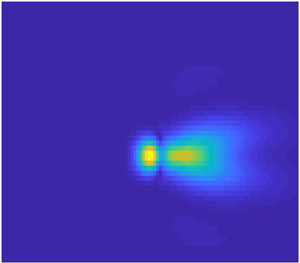
The results are displayed in figures 12–15.

Figure 12.

Contour plots for the real part of $A_{1}(X,Z)$ for angle-of-attack parameter $a = 0$ and different frequencies: (a) $\omega =1$, (b) $\omega =4$, (c) $\omega =7$ and (d) $\omega =10$. The green point represents the theoretical position of neutral oscillations.

Figure 13.

Contour plots for the real part of $A_{1}(X,Z)$ for angle-of-attack parameter $a = 1$ and different frequencies: (a) $\omega =1$, (b) $\omega =4$, (c) $\omega =7$ and (d) $\omega =10$. The green point represents the theoretical position of neutral oscillations.

Figure 14.

Contour plots for the real part of $A_{1}(X,Z)$ for angle-of-attack parameter $a = 1.139$ and different frequencies: (a) $\omega =1$, (b) $\omega =4$, (c) $\omega =7$ and (d) $\omega =10$. The green point represents the theoretical position of neutral oscillations.

Figure 15.

Contour plots for the real part of $A_1 (X,Z)$, where $\omega =10$: (a) $a=1.139$ and (b) $a=1.330$. The green point represents the theoretical position of neutral oscillations.

We first take the angle-of-attack parameter to be $a = 0$, and shift the centre of suction/blowing upstream to $X_0 = 2$. Figure 12 displays the contours of the constant real part of $A_1 (X , Z)$ (the imaginary part of $A_1 (X , Z)$ was found to behave in a similar way). One can see that with $\omega = 1.0$ the flow displays a ‘passive response’ to suction/blowing, but when $\omega$ increases, the flow becomes unstable, and the perturbations start to grow downstream of suction/blowing, taking the form of a three-dimensional wave packet. The latter is bounded in space due to the fact that the basic flow, given by $A_0 (X)$, is non-parallel. We found that the position of the maximum of the amplitude of pulsations can still be predicted with the help of equation (3.29) (see the green point plotted in figures 12–15). It is clear from figure 12 that, with increasing frequency $\omega$, the position of the maximum amplitude of the perturbations moves downstream and the number of oscillations increases. As a result, the wave packet stretches downstream. It also widens, but not significantly. Furthermore, one can see that, for different angle-of-attack parameters, the solutions behave in a similar manner (see figures 13 and 14).

Figure 15 shows how the solution changes as the angle of attack increases. The calculations were performed for $\omega = 10$. We see that the wave packet extends in both the longitudinal and spanwise directions as $a$ increases from $a = 1.139$ to $a = 1.330$. Also we observe an increase in the amplitude of the oscillations, which means that at $a = 1.330$ the boundary layer is more prone to laminar–turbulent transition.