The ability to resolve image detail is an important visual function that animals use to guide their behaviors and survive in their environments. Visual acuity can be maximized by increasing the size of the eye to enlarge the images that are projected on the photoreceptor array. The eye size of vertebrates increases with body size and its axial length can range from just 1 mm in the American toad to 107 mm in the blue whale (Hughes, Reference Hughes and Crescitelli1977; Howland et al., Reference Howland, Merola and Basarab2004). Eye size also increases with other factors such as maximum running speed probably to fulfill an important visual function, which is to avoid collisions when moving (Hughes, Reference Hughes and Crescitelli1977; Heard-Booth & Kirk, Reference Heard-Booth and Kirk2012). When comparing animals with similar size, the fast cheetah (110 km/h) has the eyes with the largest axial length among carnivores (37 mm) while the flightless penguins have the smallest among birds (21 mm). In primates, the fastest monkey (patas monkey, 55 km/h) has eyes with axial lengths (22.5 mm) that are comparable to much bigger primates such as gorillas (22.5 mm), and humans (25 mm) (Howland et al., Reference Howland, Merola and Basarab2004; Heard-Booth & Kirk, Reference Heard-Booth and Kirk2012).
Cortical visual acuity
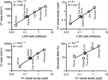
Among animals with similar eye size, visual acuity increases as a function of photoreceptor density and the number of axons from retinal ganglion cells leaving the optic nerve. Moreover, as the diameter of the optic nerve increases, the volume of the visual thalamus and primary visual cortex also becomes larger. Data from seven different mammals indicate that the primary visual cortex increases by roughly 800 mm2 for every million of LGN neurons (Fig. 1, top left). The relation is ∼400 mm2 for ∼0.5 million in cats, ∼1200 mm2 for ∼1.5 million in macaques, and ∼2400 mm2 for ∼3 million in humans (Table 1). Cortical visual acuity for central vision also increases with the number of LGN neurons (Fig. 1 top right, ∼2 cpd for one million), the size of the V1 area (Fig. 1 bottom left, ∼2 cpd for 1000 mm2) and the horizontal extent of the binocular visual field (Fig. 1 bottom right, ∼2 cpd for 50%). The relation between cortical visual acuity and binocular vision is consistent with ecological studies demonstrating a tendency for active predators with frontal eyes to have higher visual acuity than herbivores with lateral eyes (Veilleux & Kirk, Reference Veilleux and Kirk2014).
Thalamocortical visual function in different animals: primates, carnivores, scandentia, lagomorphs, and rodents. Top. The number of LGN cells is correlated to the size of area V1 (left) and cortical visual acuity (right). Bottom. Cortical visual acuity is also correlated to the size of area V1 (left, expected from correlations shown at the top), and the horizontal extent of the binocular field (shown as a percentage of the total horizontal extent of the visual field). Size of area V1 refers to only one hemisphere. See Table 1 for references.

Comparison of visual systems across different animals: primates, carnivores, scandentia, lagomorphs, and rodents. Columns 1–9 are taken from references cited below. Column 10 is calculated as column 8 times column 9; column 11 is calculated as column 10 divided by column 7; column 12 is calculated as column 6 times one million divided by column 8. Columns are numbered from left to right, from [1] for body weight to [12] for LGN-axon density in V1. All areas and volumes refer only to one hemisphere. Human: (Howland et al., Reference Howland, Merola and Basarab2004) for [1], [2]; (Curcio & Allen, Reference Curcio and Allen1990) for [3], [4], [5]; (Selemon & Begovic, Reference Selemon and Begovic2007) for [6]; (Andrews et al., Reference Andrews, Halpern and Purves1997) for [7], [8], [10]. Macaque: (Howland et al., Reference Howland, Merola and Basarab2004) for [1]; (Perry & Cowey, Reference Perry and Cowey1985) for [2]; (Kong et al., Reference Kong, Wang, Sun and Witt2010) for [3]; (Kim et al., Reference Kim, Tom and Spear1996) for [4]; (Perry & Cowey, Reference Perry and Cowey1985) for [5]; (Connolly & Van Essen, Reference Connolly and Van Essen1984) for [6]; (Malpeli & Baker, Reference Malpeli and Baker1975) for [7]; (Adams et al., Reference Adams, Sincich and Horton2007) for [8]; (Hubel & Wiesel, Reference Hubel and Wiesel1968) for [9]. Cat: (Howland et al., Reference Howland, Merola and Basarab2004) for [1], [2]; (Hughes, Reference Hughes1975) for [3], [5]; (Hughes & Wassle, Reference Hughes and Wassle1976) for [4]; (Williams et al., Reference Williams, Cavada and Reinoso-Suarez1993) for [5], [6], [7]; (Tusa et al., Reference Tusa, Palmer and Rosenquist1978) for [8]; (Hubel & Wiesel, Reference Hubel and Wiesel1962) for [9]. Tree Shrew: (Howland et al., Reference Howland, Merola and Basarab2004) for [1], [2]; (Engelmann & Peichl, Reference Engelmann and Peichl1996) for [3]; (Drenhaus et al., Reference Drenhaus, Von Gunten and Rager1997) for [4]; (Petry et al., Reference Petry, Fox and Casagrande1984) for [5]; (Conway & Schiller, Reference Conway and Schiller1983) for [6], [7]; (Sesma et al., Reference Sesma, Casagrande and Kaas1984) for [8]; (Muly & Fitzpatrick, Reference Muly and Fitzpatrick1992) for [9]. Ferret: (Howland et al., Reference Howland, Merola and Basarab2004) for [1], [2]; (Henderson, Reference Henderson1985) for [3], [4]; (Vitek et al., Reference Vitek, Schall and Leventhal1985) for [5]; (Gautschi & Clarke, Reference Gautschi and Clarke2007) for [6]; (Zahs & Stryker, Reference Zahs and Stryker1985) for [7]; (Law et al., Reference Law, Zahs and Stryker1988) for [8], [9]. Rabbit: (Howland et al., Reference Howland, Merola and Basarab2004) for [1], [2]; (Oyster et al., Reference Oyster, Takahashi and Hurst1981) for [3], [4], [5]; (Najdzion et al., Reference Najdzion, Wasilewska, Bogus-Nowakowska, Rowniak, Szteyn and Robak2009) for [6], [7]; (Hughes, Reference Hughes1971) for [8], [9]. Mouse: (Howland et al., Reference Howland, Merola and Basarab2004) for [1], [2]; (Drager and Olsen, Reference Drager and Olsen1981) for [3]; (Williams et al., Reference Williams, Strom, Rice and Goldowitz1996) for [4]; (Jeon et al., Reference Jeon, Strettoi and Masland1998) for [5]; (Seecharan et al., Reference Seecharan, Kulkarni, Lu, Rosen and Williams2003) for [6], [7]; (Garrett et al., Reference Garrett, Nauhaus, Marshel and Callaway2014) for [8]; (Antonini et al., Reference Antonini, Fagiolini and Stryker1999) for [9]. RGC: retinal ganglion cells

As the number of LGN neurons increases, the number of V1 neurons also increases but the relation is not linear (Stevens, Reference Stevens2001). V1 becomes larger than what would be expected from an equal expansion of thalamus and visual cortex. This overexpansion of area V1 makes the density of LGN axons per mm2 of cortical area to be lower in animals with larger V1 areas. The density is ∼4 times lower for the ∼1.3 million afferents of macaques (1093 axons/mm2) and the ∼3.4 million afferents of humans (1417 axons/mm2) than the ∼20,000 LGN afferents of the mouse (5000 axons/mm2) as shown in Table 1. The close relation between V1 size and LGN afferent number could explain why cortical visual acuity is better related with the number of LGN afferents (R 2 = 0.98, Fig. 1) than the retinal area (R 2 = 0.70), number of retinal ganglion cells (R 2 = 0.54), or even the peak density of retinal ganglion cells (R 2 = 0.67), as can be verified by comparing the values from Tables 1 and 2. For example, cortical visual acuity is ∼4 times higher in cats than rabbits (Table 2) but their retinal areas are similar (498 mm2 in rabbits versus 500 mm2 in cats, Table 1) and the number of retinal ganglion cells is actually ∼2 times higher in rabbits (Table 1). Such discrepancies between retinal resources and visual cortical acuity are likely to be less pronounced among animals of the same species. For example, Spanish wildcats, Felis silvestris tartessia, have higher central cone densities, higher peak density of retinal ganglion cells, more axons in the optic nerve, and more LGN neurons than domestic cats of similar weights (Williams et al., Reference Williams, Cavada and Reinoso-Suarez1993) and, since cortical visual acuity is strongly correlated with the number of LGN afferents (R 2 = 0.98, Fig. 1), Spanish wildcats should also have higher cortical visual acuity than domestic cats. Therefore, while the number of retinal ganglion cells is a good predictor of cortical visual acuity when comparing animals that are closely related, the number of LGN afferents is a better predictor when comparing species with different visual needs such as rabbits and cats. The mismatch between cortical visual acuity and retinal ganglion cell number is likely explained by differences in visual behavior. Although rabbits have more retinal ganglion cells than cats, most of these cells are likely to serve other functions than visual acuity, such as generating quick reflexes to run away from moving targets that abruptly enter their extensive visual field (Table 2) or avoiding collisions when running at fast speeds away from predators. Cats have fewer retinal ganglion cells than rabbits but more of them project to the LGN (Wassle & Illing, Reference Wassle and Illing1980; Vaney et al., Reference Vaney, Peichl, Wassle and Illing1981), which explains why the LGN volume is ∼3 times larger (Table 1) and the cortical visual acuity ∼4 times higher in cats than rabbits (Table 2).
Cortical mapping of visual space in different animals: primates, carnivores, scandentia, lagomorphs, and rodents. Columns 1–2, 5, 9–10 are taken from references cited below. Column 3 is calculated as column 2 divided by column 1 times 100; column 4 is calculated as column 8 from Table 1 divided by column 1 in this table; column 6 is calculated as column 4 times column 5; column 7 is calculated as column 1 divided by column 5; column 8 is calculated as column 2 divided by column 5. Columns are numbered from left to right as in Table 1. Macaque: (Adams et al., Reference Adams, Sincich and Horton2007) for [1], [2]; (Levitt et al., Reference Levitt, Schumer, Sherman, Spear and Movshon2001) for [5]; (De Valois et al., Reference De Valois, Albrecht and Thorell1982) for [9]; (Hubel & Wiesel, Reference Hubel and Wiesel1968) for [10]. Cat: (Sherman, Reference Sherman1974) for [1], [2]; (Cai et al., Reference Cai, Deangelis and Freeman1997) for [5]; (Movshon et al., Reference Movshon, Thompson and Tolhurst1978) for [9]; (Hubel & Wiesel, Reference Hubel and Wiesel1962) for [10]. Tree shrew: (Kaas et al., Reference Kaas, Hall, Killackey and Diamond1972) for [1], [2]; (Holdefer & Norton, Reference Holdefer and Norton1995) for [5]; (Johnson et al., Reference Johnson, Van Hooser and Fitzpatrick2010) for [9]; (Humphrey & Norton, Reference Humphrey and Norton1980) for [10]. Ferret: (Law et al., Reference Law, Zahs and Stryker1988) for [1], [2]; (Zahs & Stryker, Reference Zahs and Stryker1985) for [5]; (Baker et al., Reference Baker, Thompson, Krug, Smyth and Tolhurst1998) for [9]; (Law et al., Reference Law, Zahs and Stryker1988) for [10]. Rabbit: (Hughes, Reference Hughes1971) for [1], [2]; (Bezdudnaya et al., Reference Bezdudnaya, Cano, Bereshpolova, Stoelzel, Alonso and Swadlow2006) for [5]; (Zhuang et al., Reference Zhuang, Stoelzel, Bereshpolova, Huff, Hei, Alonso and Swadlow2013) for [9]; (Murphy & Berman, Reference Murphy and Berman1979) for [10]. Mouse: (Scholl et al., Reference Scholl, Burge and Priebe2013) for [1]; (Heesy, Reference Heesy2004) for [2]; (Tang et al., Reference Tang, Ardila Jimenez, Chakraborty and Schultz2016) for [5]; (Niell & Stryker, Reference Niell and Stryker2008) for [9]; (Drager, Reference Drager1975) for [10]. RF: receptive field

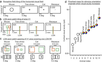
While the extent of the rabbit visual field is enormous and approaches 360 deg [(Hughes, Reference Hughes1971), Table 2], animals that need to hunt for prey (or search for small fruits) compromise the size of their visual fields to enhance binocular vision and visual acuity. This evolutionary process explains the strong correlation between cortical visual acuity and binocular field size (Fig. 1) and why the ratio between V1 size and visual field size is two orders of magnitude larger in macaques (5.95 mm2/deg) than mice (0.01 mm2/deg, Table 2). Because LGN central receptive fields are much larger in mice (6.5 deg, Table 2) than macaques (0.09 deg in parafovea and even smaller in fovea), tiling a horizontal line across the mouse visual field can be done with just 49 LGN receptive fields but it requires 2222 LGN parafoveal receptive fields in the macaque (Table 2, Fig. 2a). Similarly, a horizontal line across the binocular field requires just 6 LGN receptive fields in the mouse but 1556 in the macaque (Table 2). Interestingly, cortical visual acuity is slightly better correlated with the number of receptive fields required to tile a horizontal line in the binocular field (Table 2, R 2 = 0.87, power law with 1.27 exponent) than the tiling for the entire visual field (R 2 = 0.74, power law with 0.79 exponent), which highlights once more the intimate relation between binocular vision and cortical visual acuity.
Thalamocortical networks underlying the organization of visual cortical maps. (a) Number of non-overlapping LGN receptive fields needed to tile a horizontal line across the visual field (shown on top left corner of each rectangle, taken from column 7 in Table 2). Only 1/10 of the horizontal visual field is represented for illustration purposes. (b) Number of nonoverlapping LGN-axon-patches needed to tile a horizontal line through area V1 (shown on top left corner of each rectangle, taken from column 3 in Table 3). Green and orange colors represent two different afferents. (c) The largest spacing between two LGN-axon-patches covering one LGN receptive field in visual cortex (shown on top left corner of each rectangle, taken from column 5 in Table 3). For simplicity, axon patches are represented as squares. (d) Cortical optimal visual acuity across 11 different species (values obtained from the references cited below). Colored circles indicate pinwheel orientation maps in visual cortex. Mouse: (Niell & Stryker, Reference Niell and Stryker2008). Rat, Gray squirrel, Bush baby, Owl monkey: (Heimel et al., Reference Heimel, Van Hooser and Nelson2005). Rabbit: (Zhuang et al., Reference Zhuang, Stoelzel, Bereshpolova, Huff, Hei, Alonso and Swadlow2013). Ferret: (Baker et al., Reference Baker, Thompson, Krug, Smyth and Tolhurst1998). Tree shrew: (Johnson et al., Reference Johnson, Van Hooser and Fitzpatrick2010). Marmoset: (Forte et al., Reference Forte, Hashemi-Nezhad, Dobbie, Dreher and Martin2005). Cat: (Movshon et al., Reference Movshon, Thompson and Tolhurst1978). Macaque: (De Valois et al., Reference De Valois, Albrecht and Thorell1982). VF: visual field. RF: receptive field.

Overexpansion of the V1 thalamocortical network
Although the reduction in LGN receptive field size from mice to macaques is remarkable, the overexpansion of area V1 is even more pronounced. The ratio between V1 size and LGN receptive field size is almost one order of magnitude larger in the macaque (0.54 mm2/RF) than in the mouse (0.08 mm2/RF, Table 2) and, because the average area of an LGN axon patch is similar (mice: 0.24 mm2, macaques: 0.23 mm2, averaging all axons in mouse and parvocellular/magnocellular axons in macaques), the axon patches of LGN afferents with overlapping receptive fields must overlap in mouse cortex but can be horizontally segregated in macaque cortex (Table 3). Similarly, nearly all LGN afferents with overlapping receptive fields project to the same cortical point in rabbits [>90%, (Stoelzel et al., Reference Stoelzel, Bereshpolova, Gusev and Swadlow2008)] but at least 40% project to different cortical points in cats (Jin et al., Reference Jin, Weng, Yeh, Gordon, Ruthazer, Stryker, Swadlow and Alonso2008; Jin et al., Reference Jin, Wang, Swadlow and Alonso2011).
Comparison of LGN axon-patch density across different animals: primates, carnivores, scandentia, and rodents. Column 1 is taken from references cited below. Column 2 is calculated as the square root of column 1 times 1000; column 3 is calculated as column 8 in Table 1 divided by column 1 in this table; column 4 is calculated as column 6 in Table 1 times column 1 in this table times one million and divided by column 8 in Table 1; column 5 is calculated as the square root of the ratio between column 6 of Table 2 and column 1 of this table. Columns are numbered from left to right as in Table 1. Macaque: (Blasdel & Lund, Reference Blasdel and Lund1983) for [1]. Cat (area 17): (Humphrey et al., Reference Humphrey, Sur, Uhlrich and Sherman1985a) for [1]. Tree shrew: (Raczkowski & Fitzpatrick, Reference Raczkowski and Fitzpatrick1990) for [1]. Mouse: (Antonini et al., Reference Antonini, Fagiolini and Stryker1999) for [1]. RF: receptive field

Our understanding of the horizontal organization of the thalamocortical axon patches in cortex is still very limited in great part because reconstructions from single LGN axons are scarce. However, available measurements from macaques (Blasdel & Lund, Reference Blasdel and Lund1983), cats (Freund et al., Reference Freund, Martin and Whitteridge1985; Humphrey et al., Reference Humphrey, Sur, Uhlrich and Sherman1985a; Humphrey et al., Reference Humphrey, Sur, Uhlrich and Sherman1985b), tree shrews (Fitzpatrick & Raczkowski, Reference Fitzpatrick and Raczkowski1990; Raczkowski & Fitzpatrick, Reference Raczkowski and Fitzpatrick1990), and mice (Antonini et al., Reference Antonini, Fagiolini and Stryker1999) allow some rough estimates of axon patch coverage and spacing (Table 3). These data indicate that just 17 non-overlapping LGN-axon-patches are enough to tile a line across area V1 in mice but 5170 are needed to tile a line across area V1 in macaques (Table 3, Fig. 2b). Consequently, the largest horizontal separation between two LGN axon patches with overlapping receptive fields is less than one axon patch in mice but ∼2 axon patches in tree shrews, cats, and macaques (Table 3, Fig. 2c).
Based on these estimates, we propose that frequent separating gaps between axon patches of LGN afferents with overlapping receptive fields are a unique feature of animals with high visual acuity and have important consequences for the organization of visual cortical maps. In mice, area V1 is not large enough to allow many horizontal gaps between thalamic axon patches with overlapping receptive fields (Table 3) and the density of thalamic afferents is very high (5000 axons/mm2, Table 1). In contrast, area V1 in macaques and cats can accommodate many thalamic afferents with overlapping receptive fields that do not have overlapped patches in cortex (Table 3) and the density of thalamic afferents is ∼5 times lower than in mice (Table 1). The separating gaps between LGN axon patches with overlapping receptive fields allow sorting the thalamic afferents within the cortex by functional properties that are not just spatial position but also eye input and dark/light polarity. We argue that this more precise thalamic sorting causes a major reorganization of the visual cortical map.
Pinwheel cortical maps for stimulus orientation
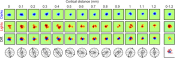
The spacing between thalamic axon patches with overlapping receptive fields is large enough in primates, carnivores, and scandentia (∼2 axon patches, Table 3) to allow clustering afferents of the same type within different cortical domains (e.g., by eye input and contrast polarity). As demonstrated by recent results (Kremkow et al., Reference Kremkow, Jin, Wang and Alonso2016; Lee et al., Reference Lee, Huang and Fitzpatrick2016), these thalamic clusters tend to rotate around each other probably to minimize the amount of wiring and cortical volume needed to represent each visual point (Mitchison, Reference Mitchison1991; Cajal, Reference Cajal1995; Chklovskii et al., Reference Chklovskii, Schikorski and Stevens2002). For example, changes in orientation preference within a horizontal track of cat visual cortex are associated with modest changes in receptive field position for one contrast polarity (OFF in Fig. 3, top row of receptive fields) and a rotation in receptive field position for the opposite polarity (ON in Fig. 3, middle row of receptive fields). In this example, the OFF receptive fields anchor the spatial position represented at the cortical domain while the ON receptive fields rotate with the changes in orientation preference (Fig. 3, bottom row of receptive fields).
Changes in orientation preference and receptive field position along a horizontal track of cat visual cortex. From top to bottom, the rows show OFF receptive fields mapped with dark stimuli (in blue), ON receptive fields mapped with light stimuli (in red), the ON–OFF receptive field difference (diff.), and the orientation/direction preference measured with moving bars (circles show the orientation preference predicted from the receptive field maps). From left to right, the columns show cortical measurements separated by 0.1 mm from 0 to 1.2 mm distance. The column on the right shows the receptive field average along the entire horizontal track (top three receptive fields) and the central positions of ON (red circles) and OFF receptive fields (blue circles). The position of these ON and OFF cortical receptive fields is determined by the receptive field population of ON and OFF thalamic afferents. Reproduced from Kremkow et al. (Reference Kremkow, Jin, Wang and Alonso2016).

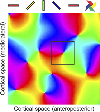
It remains unknown if such ON–OFF rotation in receptive field position is due to the mosaic organization of ON and OFF ganglion cells in the retina (Wassle et al., Reference Wassle, Boycott and Illing1981; Soodak, Reference Soodak1987; Paik & Ringach, Reference Paik and Ringach2011) or the stronger correlated firing between ON and OFF thalamic afferents (Goodhill, Reference Goodhill1993; Miller, Reference Miller1994; Goodhill & Lowel, Reference Goodhill and Lowel1995; Nakagama et al., Reference Nakagama, Saito and Tanaka2000). However, it is now clear that the ON–OFF receptive field rotation is closely related (Kremkow et al., Reference Kremkow, Jin, Wang and Alonso2016; Lee et al., Reference Lee, Huang and Fitzpatrick2016) to the pinwheel organization of cortical orientation maps [Fig. 4, (Bonhoeffer & Grinvald, Reference Bonhoeffer and Grinvald1991; Blasdel, Reference Blasdel1992; Bosking et al., Reference Bosking, Zhang, Schofield and Fitzpatrick1997; Ohki et al., Reference Ohki, Chung, Kara, Hubener, Bonhoeffer and Reid2006)], and that such pinwheel organization allows a more efficient processing of visual textures in animals with high visual acuity (Goris et al., Reference Goris, Simoncelli and Movshon2015; Koch et al., Reference Koch, Jin, Alonso and Zaidi2016). Therefore, given the close relationship between visual acuity, ON–OFF receptive field position and the pinwheel organization of cortical orientation preference, we would like to propose that pinwheel orientation maps originate when area V1 expands enough to generate high visual acuity and thalamic clustering by eye input and ON–OFF polarity.
Pinwheel pattern of the cortical map for stimulus orientation. Colors illustrate the different orientations represented on the cortical surface (cat area 17, 2 × 2 mm). A square of 0.5 × 0.5 mm is shown centered on a cortical pinwheel.

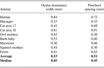
While this proposal still needs to be rigorously tested, it is consistent with available data. First, as shown here, pinwheel orientation maps emerge as cortical visual acuity increases and area V1 becomes larger (Table 2, Fig. 2d). Second, pinwheel orientation maps are not restricted to mammals but include other animals with high visual acuity. For example, barn owls have similar visual acuity to cats (Orlowski et al., Reference Orlowski, Harmening and Wagner2012) and also have pinwheel orientation maps in their visual Wulst, the avian brain structure that receives the bulk of thalamic afferents (Liu & Pettigrew, Reference Liu and Pettigrew2003). Third, all animals that have thalamic afferents sorted by eye input in area V1 (ocular dominance columns) also have pinwheel orientation maps, and the spacing between ocular dominance and pinwheel centers is remarkably similar (Table 4). Interestingly, the spacing of both ocular dominance columns and pinwheel centers is narrowly restricted to a range of about 0.4 to 0.5 mm in most animals (Table 4), and the thalamic clusters representing a single whisker in the somatosensory cortex of rodents and lagomorphs are also ∼0.5 mm wide (Woolsey & Van der Loos, Reference Woolsey and Van Der Loos1970; Bosman et al., Reference Bosman, Houweling, Owens, Tanke, Shevchouk, Rahmati, Teunissen, Ju, Gong, Koekkoek and De Zeeuw2011), which suggests a common organizing principle of sensory cortical topography. Moreover, although the thalamic axon spacing is narrowly constrained to 0.4–0.5 mm in most animals, exceptions of larger spacing (wider ocular dominance columns) are usually associated with larger distance between pinwheel centers (Table 4). For example, the cat visual cortex has several areas receiving thalamic input, and the area that has the wider ocular dominance columns, area 18, has also the larger pinwheel spacing (Table 4). Our proposal also predicts that the direction maps in the superior colliculus of frogs implanted with a third eye should be organized in a pinwheel pattern because ocular dominance bands emerge with the arrival of inputs from the third eye (Constantine-Paton & Law, Reference Constantine-Paton and Law1978), however, this prediction has not yet been tested.
Cortical spacing for ocular dominance and orientation pinwheels in area V1 of primates, carnivores, scandentia, and rodents. Column 2 is calculated as the square root of 1/pinwheel density. References for the column on the left [1] and on the right [2] are provided below. Human: (Adams et al., Reference Adams, Sincich and Horton2007) for [1]; (Yacoub et al., Reference Yacoub, Harel and Ugurbil2008) for [2]. Macaque: (Adams et al., Reference Adams, Sincich and Horton2007) for [1]; (Obermayer & Blasdel, Reference Obermayer and Blasdel1993) for [2]. Cat area 17: (Lowel, Reference Lowel1994) for [1]; (Bonhoeffer et al., Reference Bonhoeffer, Kim, Malonek, Shoham and Grinvald1995) for [2]. Cat area 18: (Lowel, Reference Lowel1994) for [1]; (Bonhoeffer & Grinvald, Reference Bonhoeffer and Grinvald1993) for [2]. Owl monkey: (Takahata et al., Reference Takahata, Miyashita, Tanaka and Kaas2014) for [1]; (Xu et al., Reference Xu, Bosking, Sary, Stefansic, Shima and Casagrande2004) for [2]. Bush baby: (Xu et al., Reference Xu, Bosking, White, Fitzpatrick and Casagrande2005) for [1], [2]. Marmoset: (Roe et al., Reference Roe, Fritsches and Pettigrew2005) for [1]; (Liu & Pettigrew, Reference Liu and Pettigrew2003) for [2]. Squirrel monkey: (Adams & Horton, Reference Adams and Horton2003) for [1]; (Obermayer & Blasdel, Reference Obermayer and Blasdel1997) for [2]. Ferret: (Law et al., Reference Law, Zahs and Stryker1988) for [1]; (Rao et al., Reference Rao, Toth and Sur1997) for [2]

Pinwheel orientation maps are found in animals with large V1 areas and LGN volumes such as macaques (1189 mm2, 77 mm3) and cats (380 mm2, 19.4 mm3) but also in tree shrews, which have a much smaller LGN volume than rabbits (2.4 mm3 versus 6 mm3, Table 1). In spite of their small LGN volume, however, tree shrews are more similar to carnivores and primates than lagomorphs in that they have large binocular fields of vision and low V1 thalamic density. The binocular field of tree shrews is similar to ferrets and two times larger than rabbits (60 deg, Table 2), and their V1 thalamic density is lower than in ferrets, rabbits, and mice (1515 axons/mm2, Table 1). The thalamic axon patches of tree shrews also have a remarkably small area (0.08 mm2, Table 3), which is almost as small as the parvocellular axon patches of the macaque [0.07 mm2, (Blasdel & Lund, Reference Blasdel and Lund1983)]. The thalamocortical organization of the tree shrew is very intriguing and, in many aspects, is radically different from that of primates, carnivores, lagomorphs, and rodents. The thalamic axon patches of tree shrews are extremely asymmetric in shape; they can spread as much 0.9 mm in the lateral dimension but only 0.14 mm in the anteroposterior dimension (Raczkowski & Fitzpatrick, Reference Raczkowski and Fitzpatrick1990). They also show a pronounced inter-ocular asymmetry, with thalamic axons from the ipsilateral eye being 3 times wider in lateral extent (and less abundant) than axons from the contralateral eye (Raczkowski & Fitzpatrick, Reference Raczkowski and Fitzpatrick1990). Finally, the thalamic afferents of tree shrews are segregated by eye input and ON–OFF polarity through the depth of the middle layers of the cortex instead of horizontally as in carnivores and primates (Harting et al., Reference Harting, Diamond and Hall1973; Hubel, Reference Hubel1975; Norton et al., Reference Norton, Rager and Kretz1985).
It is unclear why the thalamocortical pathway of tree shrews is so different. An attractive hypothesis is that cortical maps are optimized to keep all thalamic axons with overlapping receptive fields as close as possible within area V1 (Hubel & Wiesel, Reference Hubel and Wiesel1977; Durbin & Mitchison, Reference Durbin and Mitchison1990; Swindale et al., Reference Swindale, Shoham, Grinvald, Bonhoeffer and Hubener2000; Carreira-Perpinan & Goodhill, Reference Carreira-Perpinan and Goodhill2002; Kremkow et al., Reference Kremkow, Jin, Wang and Alonso2016), and this optimization requires different compromises in different animals. Perhaps, because area V1 in tree shrews is so small (66 mm2, Table 1), the best compromise is to make the thalamic axon patches as restricted as possible, sort them through the depth of layer 4, and reduce the number of ipsilateral axons while compensating the reduction by increasing its patch size. Carnivores may reach a different compromise to have both high visual acuity to search for prey and high-quality vision while running at fast speeds to hunt (110 km/h in the cheetah). The best compromise for cats may be to accommodate thalamic afferents in separate cortical areas, a large one specialized in visual acuity [area 17: 380 mm2, (Tusa et al., Reference Tusa, Palmer and Rosenquist1978)] and a smaller one specialized in processing fast movement [area 18: 98 mm2, (Tusa et al., Reference Tusa, Rosenquist and Palmer1979)]. Because running creates motion blur, cats may have a special need for Y thalamic afferents with large receptive fields and fast response latencies (Cleland et al., Reference Cleland, Dubin and Levick1971) that are also common in other animals including rodents, lagomorphs, scandentia (Sherman et al., Reference Sherman, Norton and Casagrande1975; Swadlow & Weyand, Reference Swadlow and Weyand1985; Price & Morgan, Reference Price and Morgan1987; Krahe et al., Reference Krahe, El-Danaf, Dilger, Henderson and Guido2011), and primates (Schiller & Malpeli, Reference Schiller and Malpeli1978; Kaplan & Shapley, Reference Kaplan and Shapley1982). However, the receptive fields of Y afferents projecting to area 18 in cats are 2–3 times larger than those from afferents projecting to area 17 (Yeh et al., Reference Yeh, Stoelzel and Alonso2003). Therefore, such Y afferents would have to cover a huge cortical region if they projected to area 17 (∼2 mm2/deg, Table 2) but can remain more restricted (although still large) within area 18, which is ∼4 times smaller and has a much coarser retinotopic precision (∼0.5 mm2/deg). Interestingly, in spite of such unique cortical specialization, thalamic axon patches are larger in cats than in any other animal studied to date (Table 3, Fig. 2).
Concluding remarks
The thalamocortical pathway plays an important role in building visual cortical maps and maximizing visual spatial resolution within the cerebral cortex. During evolution, the expansion of primary visual cortex is associated with an increase in visual acuity, a reduction in the cortical density of thalamic afferents, and an increase in the cortical separation between axon patches of thalamic afferents with overlapping receptive fields. This increased separation allows sorting thalamic afferents within the visual cortex not only by their spatial position but also by their eye input and contrast polarity (ON or OFF). We propose that this increased separation between thalamic axon patches, and the resulting thalamic sorting, leads to a major reorganization of the visual cortical map and allows for the emergence of a pinwheel pattern in the cortical representation of stimulus orientation. While this proposal is consistent with available data, anatomical reconstructions from single thalamic axons remain unfortunately scarce, which limits our ability to build realistic models of cortical architecture. It is surprising that, in the era of the connectome, we still have to rely on heroic reconstructions from single thalamic axons obtained more than two decades ago with more limited resources. Advancing progress in understanding thalamocortical processing would greatly benefit from a renewed effort to fully reconstruct the thalamocortical network, which provides the structural framework for visual function.
Acknowledgment
Supported by NIH grants EY027157 (RM) and EY05253 (JMA).