



1. Introduction
Intermittent swimming, also known as burst-and-coast swimming, is a common swimming style employed by various fish species. During the burst phase, fish propel themselves using a body wave, while in the coast phase, they decelerate by maintaining a straight body without muscular activation (Weihs Reference Weihs1974; Videler & Weihs Reference Videler and Weihs1982). This behaviour is observed across diverse species, growth stages and situations (Videler & Weihs Reference Videler and Weihs1982; McHenry & Lauder Reference McHenry and Lauder2005; Wu et al. Reference Wu, Yang and Zeng2007; Gellman et al. Reference Gellman, Tandler and Ellerby2019; Li et al. Reference Li, Ashraf, François, Kolomenskiy, Lechenault, Godoy-Diana and Thiria2021; Coughlin et al. Reference Coughlin, Chrostek and Ellerby2022).
Intermittent swimming may offer several advantages. First, the coast phase stabilizes self-generated flow perturbations, enhancing sensory capabilities and avoiding alerting potential prey and predators (Teyke Reference Teyke1985; Windsor et al. Reference Windsor, Tan and Montgomery2008; Mogdans Reference Mogdans2019). Second, white fibres used in high-speed swimming fatigue rapidly, and intermittency may assist in recovery and sustain locomotion (Videler & Weihs Reference Videler and Weihs1982). Finally, modulation of coasting duration offers an alternative for controlling mean swimming speed without significant changes in tail-beat amplitude and frequency, potentially optimizing muscle efficiency (Gellman et al. Reference Gellman, Tandler and Ellerby2019; Li et al. Reference Li, Ashraf, François, Kolomenskiy, Lechenault, Godoy-Diana and Thiria2021).
In addition to the factors mentioned above, energy efficiency is also considered a primary motivation for intermittent swimming. Based on the Bone–Lighthill boundary-layer thinning mechanism, Lighthill (Reference Lighthill1971) originally proposed that the skin friction drag on an undulating body is 3–5 times larger than that on a coasting body. Therefore, a fish can reduce its mean skin friction by alternating between burst and coast phases. Inspired by this theory, Weihs (Reference Weihs1974) developed a dynamical model to calculate the energy expenditure of fish swimming, with the key parameter being the ratio ( $\beta$) of drag during active swimming to drag during passive coasting. Intermittent swimming is energetically advantageous for
 $\beta \gt 1$, with a larger
 $\beta$ indicating a greater energy advantage. Weihs (Reference Weihs1974) demonstrated that with
 $\beta =3$ as suggested by Lighthill (Reference Lighthill1971), intermittent swimming yields an energy saving of over
 $50\, \%$ compared with continuous swimming at the same mean speed. Building on this model, Videler & Weihs (Reference Videler and Weihs1982) established a relationship between energy expenditure and the initial and final swimming speeds of burst swimming. By analysing kinematic data of cod and saithe fish, they showed that fish choose initial and final burst speeds corresponding to predicted optimal energy expenditure. Wu et al. (Reference Wu, Yang and Zeng2007) estimated passive and active drag by linking a vortex-ring model constructed from digital particle image velocimetry results with kinematic data from koi carp. Using these drag coefficients, they estimated an energy saving of nearly
 $45\, \%$ when koi carp utilize intermittent swimming. Recently, an additional inviscid Garrick mechanism (Akoz & Moored Reference Akoz and Moored2018; Akoz et al. Reference Akoz, Han, Liu, Dong and Moored2019, Reference Akoz, Mivehchi and Moored2021) was discovered, in accordance with Garrick’s linear theory (Garrick Reference Garrick1936). This mechanism relies on the trade-off between thrust-producing forces due to added mass and circulatory forces that induce drag, resulting in energy savings of up to
 $10\,\%$–
 $30\,\%$ in a viscous flow.
Some numerical simulations and model experiments have confirmed the energy advantage of intermittent swimming. Chung (Reference Chung2009) conducted two-dimensional numerical simulations of intermittent swimming, assuming that the burst phase consists of a single tail beat. The results demonstrated that intermittent swimming can save over  $50\, \%$ energy compared to continuous swimming, with only a slight decrease in swimming speed. Water tunnel experiments on a nominally two-dimensional pitching foil also supported the energetic advantage of intermittent motions over continuous motions (Floryan et al. Reference Floryan, Van Buren and Smits2017).
However, there are disagreements regarding the energy advantage. Dai et al. (Reference Dai, He, Zhang and Zhang2018) and Liu et al. (Reference Liu, Huang and Lu2020) numerically studied intermittent swimming of elastic swimmers, and found that intermittent style is more economical than continuous style only when the cruising Reynolds number is sufficiently large and the duty cycle (the ratio of burst duration to coast duration) is moderate. Ashraf et al. (Reference Ashraf, Van Wassenbergh and Verma2020) examined power requirements for various realistic undulating kinematics extracted from video recordings of live fish, showing that continuous swimming consumes considerably less mechanical energy than intermittent modes at comparable speeds. Gupta et al. (Reference Gupta, Thekkethil, Agrawal, Hourigan, Thompson and Sharma2021) investigated the energy efficiency of self-propelled hydrofoils for various modes, and suggested that intermittent swimming is effective for carangiform and thunniform tail-like kinematics but not for anguilliform body-like kinematics. Li et al. (Reference Li, Ashraf, François, Kolomenskiy, Lechenault, Godoy-Diana and Thiria2021) described the kinematics of real fish swimming in a water flume from low to high speed regimes, finding that fish sustain the demanded speed by modifying the duty cycle instead of tail-beat frequency and amplitude.
Recently, Kang et al. (Reference Kang, Gong, Lu, Cui and Fan2023) formulated a reduced-order dynamical model for intermittent swimming, uncovering scaling laws connecting swimming performance to body kinematics, revealing that the energy efficiency of intermittent swimming is not inherently superior to continuous swimming, and depends on the parameter  $\beta$. Li et al. (Reference Li, Kolomenskiy, Liu, Godoy-Diana and Thiria2023) utilized a hybrid computational dynamic model with a ‘gait assembly’ approach to generate arbitrary burst-and-coast gaits and assess swimming performance. Their findings indicate that while burst-and-coast swimming can be more energy-efficient than continuous swimming, an unoptimized gait may be highly energetically costly.
We note that the majority of the numerical simulations and model experiments have confirmed the energy advantage of intermittent swimming for high Reynolds number swimming, but not for low Reynolds number swimming. But one still cannot draw a direct conclusion that the intermittent swimming in a low Reynolds number regime is energetically inefficient, since these researches have relied on simplified body kinematics that could neglect some important dynamic aspects of live-fish swimming. First, in the above studies, the body kinematics of the swimmer is fixed and does not respond to the change of the environment, while the routine locomotor behaviour of most fishes is intrinsically unsteady and constantly adjusted to adapt to the environmental change. Second, the tail-beat frequency is assumed to be constant, while a certain degree of variation in tail-beat frequency is observed in several live fish experiments. For example, Borla et al. (Reference Borla, Palecek, Budick and O’Malley2002) found that the tail-beat frequency of larval zebrafish when approaching a prey intermittently varies between  $25\, \rm Hz$ and
 $80\, \rm Hz$.
The application of deep reinforcement learning (DRL) in biological propulsion simulations can bridge the gap between previous simplified models and real fish or bionic robots to some extent by dynamically adjusting body kinematics, which includes responding to environmental changes and variations in tail-beat amplitude and frequency. And some studies have shown its high promise in bionic propulsion (Xue et al. Reference Xue, Han, van Oorschot, Clifton and Fan2023; Cui et al. Reference Cui, Sun, Zhu, Yang, Zhang, Cui, Fan and Wang2024). Gazzola et al. (Reference Gazzola, Hejazialhosseini and Koumoutsakos2014b) pioneered the use of reinforcement learning in a self-propelled system to train multiple swimmers to swim in a cyclic manner. Subsequently, Yan et al. (Reference Yan, Chang, Tian, Wang, Zhang and Liu2020, Reference Yan, Chang, Wang, Tian, Zhang and Liu2021) demonstrated that a single self-propelled fish model can learn to navigate different trajectories and avoid obstacles through DRL training. Zhu et al. (Reference Zhu, Tian, Young, Liao and Lai2021, 2022c) and Zhu & Pang (Reference Zhu and Pang2023) conducted numerical investigations on the navigation and rheotaxis process of fish-like swimmers in both still water and vortical flow using DRL. Mandralis et al. (Reference Mandralis, Weber, Novati and Koumoutsakos2021) utilized reinforcement learning to uncover escape patterns for larval fish under energy constraints, and identified patterns resembling C-start swimming. Novati et al. (Reference Novati, Verma, Alexeev, Rossinelli, Van Rees and Koumoutsakos2017) employed DRL in a two self-propelled swimmers system for the first time to optimize the follower’s kinematics and minimize its lateral displacement from the leader. Verma et al. (Reference Verma, Novati and Koumoutsakos2018) further achieved active control of a fish school by modifying the motion of downstream bodies to enhance efficiency. Yu et al. (Reference Yu, Liu, Wang, Liu, Lu and Huang2022) and Zhu et al. (Reference Zhu, Pan and Tian2022a) discovered that stable schooling formations arise from the synergistic effects of active control and passive self-organization. Moreover, Zhu et al. (Reference Zhu, Pan and Tian2022a) demonstrated that swimmers trained with multi-agent DRL can withstand strong hydrodynamic forces to maintain dense formations while swimming along desired paths.
This work investigates the continuous and intermittent swimming of a larval zebrafish-like swimmer. It differs from the above intermittent swimming studies in several important aspects. First and foremost, instead of using a fixed-gear swimming kinematics, a feedback control strategy is developed by optimizing the cost of transport, thereby allowing a flick-to-flick (one half-cycle tail beat) adjustment of the body kinematics in real time. Through this approach, the observed intermittent motion behaviour is the result of autonomous training and learning by fish, which was not predetermined. Second, we study trained swimming using both fixed and variable tail-beat frequencies, leading to different optimal swimming behaviours due to the varying constraints imposed on body kinematics. In contrast to previous constrained intermittent swimming models, which use a sinusoidal function to describe a symmetric burst mode (Floryan et al. Reference Floryan, Van Buren and Smits2017; Akoz & Moored Reference Akoz and Moored2018; Liu et al. Reference Liu, Liu and Huang2022; Kang et al. Reference Kang, Gong, Lu, Cui and Fan2023), the trained motion with variable tail-beat frequencies is characterized by an asymmetric burst phase, featuring slow forward and fast backward tail flicks, followed by a coast phase. Remarkably, despite the wide range of motion function parameters (including significant variations in amplitudes and periods), the DRL results align well with theoretical predictions when estimated using scaling laws.
The rest of the paper is structured as follows. Section 2 introduces the physical model, the immersed boundary–lattice Boltzmann method and the DRL approach. Section 3 discusses the results in three parts: (i) the simulation settings and training performance; (ii) the swimming performance of trained fish with both fixed and variable tail-beat periods; (iii) the scaling laws for trained fish to link crucial parameters, including cruising Reynolds number, thrust, swimming number, and cost of transport. Concluding remarks are given in § 4.
A schematic of the fish model: (a) ventral view of a larval zebrafish (Yao et al. Reference Yao, Xu, Zhou and Xu2018); (b) constructed shape of the two-dimensional model; (c) illustration of the motion of the swimmer. Here,  $L$ is the length of the fish,
 $l$ is the arc length along the mid-line of the body,
 $(x,y)$ represents the global coordinate system, while
 $(x_l, y_l)$ signifies the local coordinate system, whose origin is positioned at the head of the fish,
 $d$ is the half-thickness of the body,
 $r_{tip}$ is the distance between the head of the fish and the target,
 $\theta _{tip}$ is the orientation angle of the swimmer with respected to the target,
 ${\boldsymbol{r}}_c$ and
 $\theta$ are the position vector and the body rotation angle around the mass centre, respectively,
 ${\boldsymbol{F}}_t$ and
 $M_z$ are the total hydrodynamic force on the fish body and the total hydrodynamic torque on the centre of mass, respectively, and
 $h_l$ and
 $\theta _l$ are the lateral displacement and deflection angle of the mid-line with respect to the
 $x_l$-axis, respectively.

2. Physical model and methodology
2.1. Kinematic model of the fish
The shape of the two-dimensional swimmer is close to the cross-section of a larval zebrafish as shown in figures 1(a) and 1(b). The half-thickness of the body ( $d$) is estimated mathematically by
 \begin{equation} d = \left \{ \begin{array}{ll} 0.075\sqrt {1-\dfrac {(l/L-0.107)^2}{0.107^2}}, & 0\leqslant l/L\lt 0.2, \\[3pt] 0.043-0.0295 l/L, & 0.2\leqslant l/L\lt 0.95, \\[3pt] 0.3-0.3 l/L, & 0.95\leqslant l/L \leqslant 1.0, \end{array} \right . \end{equation}
where  $l$ is the arc length along the mid-line of the body, and
 $L$ is the body length, which is a constant during the swimming (Tian Reference Tian2015).
The kinematics of the fish body is composed of the body undulation in the local coordinate system ( $h_l$ and
 $\theta _l$ in the
 $x_l$–
 $y_l$ system), the translation of the mass centre (
 ${\boldsymbol{r}}_c$), and the the body rotation around the mass centre (
 $\theta$). The undulatory motion is controlled by the fish itself, which can be taken as the superposition of different waves propagating from head to tail. A polynomial-based waveform is adopted for each wave, and the kinematics of the newest generated waves can be changed every half-cycle. In the
 $n$th half-cycle, the mid-line lateral displacement
 $h_l$ is determined by
 \begin{equation} h_l(l,t)=\int ^{l}_0 \sin (\theta _l)\,{\rm d}l, \end{equation}
 \begin{equation} \theta _l(l,t)=\max \big[0,\left (l/L-0.2\right )^3\big] f_w\left (\frac {\lambda _n}{T_n}(t-t_{0n})-\frac {l}{L}\right ), \end{equation}
where  $\theta _l$ is the deflection angle of the mid-line with respect to the
 $x_l$-axis as shown in figure 1(c),
 $\lambda _n$ is the wavelength of the
 $n$th half-wave,
 $T_n$ is the period of the
 $n$th half-wave,
 $t$ is the time,
 $t_{0n}=0$ for
 $n=1$ and
 $\sum _{i=1}^{n-1}T_i$ for
 $n\gt 1$, and
 $f_w$ is the waveform function described by
 \begin{equation} f_w(\zeta )=c_{0}+c_{1}\zeta +c_{2}\zeta ^{2}+c_{3}\zeta ^{3}+c_{4}\zeta ^{4}+c_{5}\zeta ^{5}, \end{equation}
where  $c_{i}$ (
 $i=0,1, \ldots ,5$) can be determined by
 $f_w(0)=(\theta _{l {max}})_{n-1}$,
 $f_w(\lambda _n/2)=(\theta _{l {max}})_n$,
 $f'_{\!\!w}(0)=f'_{\!\!w}(\lambda _n/2)=0$,
 $f''_{\!\!\!\!w}(0)=-f_w(0)\,(2\pi /\lambda _{n-1})^2$ and
 $f''_{\!\!\!w}(\lambda _n/2)=-f_w(\lambda _n/2)\,(2\pi /\lambda _n)^2$, and
 $(\theta _{l {max}})_n$ is the maximum deflection angle at the tail tip of the
 $n$th half-wave. In this definition, the head is always kept rigid (
 $l/L\lt 0.2$), and the deflection of the tail is obvious only in the posterior part, which is similar to the ‘J-turn’ body kinematics of larval zebrafish as described in Borla et al. (Reference Borla, Palecek, Budick and O’Malley2002) and McElligott & O’ Malley (Reference McElligott and O’Malley2005). This model allows the swimmer to change its periods (
 $T_n$), amplitudes (
 $\theta _{l {max}}$) and wavelengths (
 $\lambda _n$) smoothly and arbitrarily every flick. For clarity, ‘one flick’ is defined as a half-cycle tail beat, as noted in Muller et al. (Reference Müller, Stamhuis and Videler2000) and Wu et al. (Reference Wu, Yang and Zeng2007). Consequently, the
 $n$th flick corresponds to the behaviour exhibited in the
 $n$th half-cycle. Therefore, the swimmer is able to choose appropriate combinations of different kinematics to achieve different manoeuvring movements such as accelerating, decelerating and yawing.
The translational and rotational motions of the fish are governed by the fluid–structure interaction in the global coordinate system  $(x,y)$ according to Newton’s law of motion:
 \begin{equation} m\,\dfrac { \textrm {d}^2{\boldsymbol{r}}_c}{ \textrm {d}t^2}={\boldsymbol{F}}_t, \end{equation}
 \begin{equation} \frac { \textrm {d}}{ \textrm {d}t}\left (I_z\,\frac { \textrm {d}\theta }{ \textrm {d}t}\right )=M_z, \end{equation}
where  $m$ represents the mass of the fish,
 $I_z$ is the inertia moment of the centre of the mass,
 ${\boldsymbol{F}}_t$ is the total hydrodynamic force acting on the fish body,and
 $M_z$ is the total hydrodynamic torque exerted on the centre of mass.
2.2. Immersed boundary–lattice Boltzmann method for the fluid–structure interaction system
The fluid motion is governed by the incompressible Navier–Stokes equations
 \begin{equation} \frac { {\partial }{\boldsymbol{u}}}{ {\partial } t}+{\boldsymbol{u}}\boldsymbol{\cdot} \boldsymbol{\nabla} {\boldsymbol{u}}=-\frac {1}{\rho }\,\boldsymbol{\nabla} p+\nu\, \nabla ^2{\boldsymbol{u}}+{\boldsymbol {f}}_b, \end{equation}
 \begin{equation} \boldsymbol{\nabla} \boldsymbol{\cdot} {\boldsymbol{u}}=0, \end{equation}
where  $\boldsymbol{u}$ is the velocity,
 $p$ is the pressure,
 $\rho$ is the density, and
 $\nu$ is the fluid kinematic viscosity. The body force
 ${\boldsymbol {f}}_b$ represents an interaction force applied to enforce the no-slip velocity boundary condition.
The lattice Boltzmann method (LBM) is used to simulate the fluid dynamics (Xu et al. Reference Xu, Tian, Young and Lai2018; Huang & Tian Reference Huang and Tian2019). Instead of solving the Navier–Stokes equations directly, the LBM solves the discrete lattice Boltzmann equation that governs the kinematics of the mesoscopic particles,
 \begin{equation} f_i(\boldsymbol {x}+\boldsymbol {c}_i\,\triangle t,t+\triangle t)-f_i(\boldsymbol {x},t)={\Omega }_i(\boldsymbol {x},t)+\triangle t\,G_i(\boldsymbol {x},t), \quad i=0,\ldots ,8, \end{equation}
where  $f$ is the particle density distribution function,
 $\boldsymbol {x}=(x,y)$ is the space coordinate,
 $\boldsymbol {c_i}$ is the discrete lattice velocity, and
 $\triangle t$ is the time step. Here,
 ${\Omega }_i$ and
 $G_i$ are the collision operator and the source term representing the body force, respectively, which are obtained by
 \begin{equation} \Omega _i=-(\hat {M}^{-1}\hat {S}\hat {M})_{ij}(f_i-f_i^{eq}), \end{equation}
 \begin{equation} G_i=[\hat {M}^{-1}(\hat {I}-\hat {S}/2)\hat {M}]_{ij}F_j, \end{equation}
where  $\hat {M}$ is a
 $9\times 9$ transformation matrix, and
 $\hat {S}$ and
 $\hat {I}$ represent, respectively, the relaxation matrix and identity matrix. Also,
 $f_i^{eq}$ and
 $F_i$ are the equilibrium distribution function and the effect of fluid body force, respectively, which are determined by
 \begin{equation} f_i^{eq}=w_i\rho \left [1+\frac {{\boldsymbol{u}}\boldsymbol{\cdot} {\boldsymbol {c}}_i}{c_s^2}+\frac {({\boldsymbol{u}}\boldsymbol{\cdot} {\boldsymbol {c}}_i)^2}{2c_s^4}-\frac {{\boldsymbol{u}}\boldsymbol{\cdot} {\boldsymbol{u}}}{2c_s^2}\right ], \end{equation}
 \begin{equation} F_i=w_i\left (\frac {{\boldsymbol {c}}_i-{\boldsymbol{u}}}{c_s^2}+\frac {{\boldsymbol {c}}_i\boldsymbol{\cdot} {\boldsymbol{u}}}{c_s^4}c_i\right )\boldsymbol{\cdot} {\boldsymbol {f}}_b, \end{equation}
where  $w_i$ is the weighting coefficient, and
 $c_s=\triangle x/(\sqrt {3}\,\triangle t)$ is the lattice speed of sound, with
 $\triangle x$ the lattice spacing. In this simulation, the D2Q9 model is used, of which
 $\hat {M}$ and
 $\hat {S}$ matrices can be found in Lallemand & Luo (Reference Lallemand and Luo2000) and Kruger et al. (Reference Krüger, Kusumaatmaja, Kuzmin, Shardt, Silva and Viggen2017). Also,
 $w_0=4/9$,
 $w_1=w_2=w_3=w_4=1/5$,
 $w_5=w_6=w_7=w_8=1/36$, and
 $c_0, \ldots , c_8$ are
 $(0,0)$,
 $(\pm 1, 0)$,
 $(0, \pm 1)$,
 $(\pm 1, \pm 1)$, respectively.
Once the particle density distribution  $f$ is known, the macroscopic physical quantities such as fluid density, pressure and velocity can be computed from
 \begin{equation} \rho =\sum f_i,\quad p=\rho c^2_s, \quad \boldsymbol {u}=\frac {1}{\rho }\left (\sum {f_i\boldsymbol {c}_i}+\frac {\triangle t\, \boldsymbol {f}_b}{2}\right ). \end{equation}
The viscous stress tensor  $\sigma _{\alpha \beta }$ and fluid force density on the boundary
 ${\boldsymbol{F}}_f$ in the new step are calculated with
 \begin{equation} \sigma _{\alpha \beta }=-\sum \big[\hat {M}^{-1}(\hat {I}-\hat {S}/2)\hat {M}\big]_{ij}\big(f_j-f_j^{eq}+F_j\big)c_{i\alpha }c_{i\beta }, \end{equation}
 \begin{equation} F_{f\alpha }=(\sigma _{\alpha \beta }-p\delta _{\alpha \beta })n_{B\beta }, \end{equation}
where  $\delta _{\alpha \beta }$ is the Kronecker delta,
 $n_{B\beta }$ is the outer normal vector of the boundary
 $S_B$, and
 $\alpha$ and
 $\beta$ are dummy indices.
The total force  ${\boldsymbol{F}}_t$ and moment
 $M_z$ on the swimmer model can be computed with
 \begin{equation} {\boldsymbol{F}}_t(t)=\int _{S_B}{\boldsymbol{F}}_f\, {\rm d}s,\quad M_z(t)=\int _{S_B}{\boldsymbol{F}}_f\times ({\boldsymbol{X}}-{\boldsymbol{r}}_c)\boldsymbol{\cdot} {\boldsymbol {e}}_z\, {\rm d}s, \end{equation}
and the input power performed by the surface of the body on the surrounding fluid is calculated with
 \begin{equation} P(t)=-\int _{S_B}{\boldsymbol{F}}_f\boldsymbol{\cdot} \frac {\partial {\boldsymbol{X}}}{\partial t}\,{\rm d}s, \end{equation}
where  $s$ is the arc length along the surface of the swimmer,
 $\boldsymbol{X}$ is the Lagrangian coordinate on the fish surface, and
 ${\boldsymbol {e}}_z$ is the unit vector along the
 $z$-axis.
In addition, a diffusion immersed boundary method (IBM) (Ma et al. Reference Ma, Wang, Young, Lai, Sui and Tian2020; Huang & Tian Reference Huang and Tian2019; Xu et al. Reference Xu, Tang, Tian, Peng, Xu and Zeng2014; Huang et al. Reference Huang, Tian, Young and Lai2021) is utilized to handle the boundary condition at the fluid–structure interface according to
 \begin{equation} {\boldsymbol{F}}_{IB}({\boldsymbol{X}})=\eta \big[{\boldsymbol{u}}_B({\boldsymbol{X}})-\int _{V_f}{\boldsymbol{u}}({\boldsymbol {x}})\,\delta ({\boldsymbol{X}}-{\boldsymbol {x}})\,{\rm d}{\boldsymbol {x}}\big], \end{equation}
 \begin{equation} {\boldsymbol {f}}_{b,IB}=\int _{S_B}{\boldsymbol{F}}_{IB}({\boldsymbol{X}})\,\delta ({\boldsymbol{X}}-{\boldsymbol {x}})\,{\rm d}s, \end{equation}
where  ${\boldsymbol{F}}_{IB}$ represents the Lagrangian force on the immersed boundary,
 ${\boldsymbol {f}}_{b,IB}$ is the fluid body force due to the boundary,
 $\eta$ is the feedback coefficient, of which the value is determined by the body geometry (Xu et al. Reference Xu, Tian, Young and Lai2018, Reference Xu, Wang, Tian, Young and Lai2019),
 ${\boldsymbol{u}}_B$ represents the prescribed velocity of the boundary surface, and
 $S_B$ and
 $V_f$ are the boundary surface of the fish body and the fluid domain, respectively. In numerical simulations,
 $\delta$ is approximated with a kernel function
 \begin{equation} \triangle (x,y)=\frac {1}{\triangle x^2}\,\phi \left (\frac {x}{\triangle x}\right )\,\phi \left (\frac {y}{\triangle y}\right ), \end{equation}
 \begin{equation} \phi (x) = \left \{ \begin{array}{ll} \dfrac {1}{4}\left [1+\cos \left (\dfrac {\pi x}{2}\right )\right ], & 0\leqslant x\leqslant 2, \\[3pt] 0, & 2\leqslant x. \end{array} \right . \end{equation}
Compared to body conformal methods (Tian Reference Tian2014; Tian et al. Reference Tian, Bharti and Xu2014, Reference Tian, Wang, Young and Lai2015), the grid generation in the IBM is much easier for complicated shapes (Mittal & Iaccarino Reference Mittal and Iaccarino2005; Sotiropoulos & Yang Reference Sotiropoulos and Yang2014; Huang & Tian Reference Huang and Tian2019). And a multi-block geometry-adaptive Cartesian grid is coupled with the IBM–LBM to accelerate the computation. As shown in figure 2, the present simulation is performed in a rectangular computational domain  $148L\times 148L$, which is divided into 8 blocks with approximately
 $56.8\times 10^3$ initial points. The minimum non-dimensional grid spacing is
 $\triangle x/L=\triangle y/L=0.01$ near the inner boundaries, and the non-dimensional time step size is
 $\triangle t/T=0.001$. A detailed description of this numerical scheme and its validation can be found in Xu et al. (Reference Xu, Tian, Young and Lai2018, Reference Xu, Wang, Tian, Young and Lai2019), Ma et al. (Reference Ma, Wang, Young, Lai, Sui and Tian2020), Young et al. (Reference Young, Tian, Liu, Lai, Nadim and Lucey2020), Zhu et al. (Reference Zhu, Tian, Young, Liao and Lai2021) and Tian et al. (Reference Tian, Luo, Zhu, Liao and Lu2011).
Baseline grids used in the simulation: (a) full and (b) partial computational domains.

The reinforcement learning framework in fish swimming towards a target. The agent is the DRQN; the environment is the fluid–structure interaction simulation using the IB–LBM; the action is the adjustment of swimming motion; the reward is to reduce the energy expenditure; states are distance and orientation angle to the target, and action.

2.3. The DRL approach
The DRL method is a machine learning method combining reinforcement learning with an artificial neural network. DRL has gained extensive attention due to its success in complex real-world problems (Mnih et al. Reference Mnih2015), recently in fluid-related problems (Fan et al. Reference Fan, Yang, Wang, Triantafyllou and Karniadakis2020; Vignon et al. Reference Vignon, Rabault and Vinuesa2023; Wang et al. Reference Wang, Lin, Zhao, Chen, Guo, Yang, Wang and Fan2024b). In this study, a specific DRL method called deep recurrent Q-network (DRQN) (Hausknecht & Stone Reference Hausknecht and Stone2015) is adopted, in which a three-layer long short-term memory recurrent neural network (LSTM-RNN) is used to process time-sequential data.
In this method, a smart agent learns to achieve a specific goal by interacting with its environment (Colabrese et al. Reference Colabrese, Gustavsson, Celani and Biferale2017). The RL framework in this study is shown in figure 3, where the agent is represented by an artificial neural network (DRQN) and the environment corresponds to the fluid–structure interaction simulation of fish swimming towards to a target with the immersed boundary–lattice Boltzmann method (IB–LBM). The interaction procedure between the IB–LBM and the DRQN is divided into a sequence of discrete steps  $n=0,1,2,3,\ldots$. At each time step
 $n$, the agent receives states of the environment (denoted by
 $s_n$) and takes actions (denoted by
 $a_n$) that are determined based on the states and exerted on the environment. Finally, the agent will receive a reward (denoted by
 $rd_{n+1}$) for each action, indicating the quality of the previous actions. The core idea is that the agent tries different actions in different states, and finds a policy (denoted by
 $\pi (s_n,a_n)$, which describes the probability of selecting each action in each state) that maximizes the long-term reward (the action-value function):
 \begin{equation} Q(s_n,a_n)=E[r{d}_{n+1}+\gamma r{d}_{n+2}+\gamma ^2 r{d}_{n+3}+\gamma ^3 r{d}_{n+4}+\cdots \mid s_n,a_n], \end{equation}
where  $E$ is the expectation,
 $rd_{n+1}$ is the reward of the
 $n$th action,
 $rd_{n+2}$,
 $rd_{n+3}$ and
 $rd_{n+4}$ are the subsequent rewards, and
 $\gamma$ is the discount rate, ranging from 0 to 1. If
 $\gamma =0$, then the agent maximizes only the immediate rewards. If
 $\gamma =1$, then the agent maximizes the sum of all rewards. For all cases in this paper,
 $\gamma$ is chosen to be
 $0.99$ as in Mnih et al. (Reference Mnih2015).
In this work, an LSTM-RNN with three 64-LSTM-cell layers and a linear output layer is adopted to approximate the action-value function. The neural network is updated iteratively by minimizing the temporal difference error
 \begin{equation} T{D}_{err}=r{d}_{n+1}+\gamma\, Q^*(s_{n+1},a^*_{n+1})-Q(s_n,a_n), \end{equation}
where  $Q^*(s,a)$ is the optimal action-value function, i.e.
 $Q^*(s_{n+1},a^*_{n+1})=\max_{a}Q(s_{n+1},a)$ for all actions in state
 $s_{n+1}$, and
 $a^*$ is the optimal action maximizing
 $Q$. This can be achieved by updating the network weights via gradient descent methods,
 \begin{equation} ws_i=ws_i-\xi\, \frac {\partial {(T{D}_{err})}^2}{\partial (ws_i)}. \end{equation}
Here,  $ws_i$ is the weight of the network, while
 $\xi$ denotes the learning rate, which is set to
 $0.001$. A detailed description of the updating procedure can be found in Zhu et al. (Reference Zhu, Tian, Young, Liao and Lai2021).
3. Results and discussion
3.1. Simulation setup and performance of training
As shown in figure 3, a self-propelled fish is trained to reach a static target from random distances and orientations, which simulates the process whereby a larval zebrafish captures a prey. For simplicity, the swimmer of length  $L$ is restricted in a circular area with radius
 $R=10L$ and centre at the original point
 $O$ of the global
 $(x,y)$ system. The target is also placed at the centre point
 $O$.
We have a particular interest in the efficiency of a wide variety of ‘swimmers’, including real fish and robots, as well as oscillating foils/flexible plates. For a body in steady self-propelled motion or free swimming, the time-averaged net propulsion force is zero, and it is difficult to distinguish precisely between thrust and drag (Ren et al. Reference Ren, Yu, Li and Feng2022), so the Froude efficiency can no longer be defined. In such a case, the cost of transport  $COT$ is a useful performance metric, which is widely used in biology (Fish & Rohr Reference Fish and Rohr1999; Bale et al. Reference Bale, Hao, Bhalla and Patankar2014). Specifically, the cost of transport is defined as
 \begin{equation} COT=\bar {P}/m\bar {U}, \end{equation}
where  $\bar {P}$ and
 $\bar {U}$ are the mean power consumption and mean velocity, respectively. The minimum
 $COT$ is assumed to occur at the velocity at which the animal can cover the largest distance for the smallest energy cost (Smits Reference Smits2019).
In the current setting, to reach the target with lowest energy expenditure, the reward is defined as
 \begin{equation} r{d}=-\frac {\hat {u}_r}{\hat {P}}, \end{equation}
where  $\hat {u}_r$ and
 $\hat {P}$ are the mean swimming velocity and mean energy consumption of the swimmer towards the target, evaluated over the interval of two successive actions.
The swimmer propels itself by flapping its tail from one side to the other with ‘J-turn’-like kinematics, as defined by (2.2). In order to achieve high manoeuvrability and efficiency, the swimmer can change the tail-beat amplitude and period every flick (half-cycle tail beat). Each time the fish chooses a parameter, it is considered to be taking an action. The fish can choose tail-beat periods (consisting of two tail flicks) from the set of values  $\{0.6T, 0.8T, T, 1.2T, 1.4T\}$, where
 $T$ is the characteristic time representing the average period. The duration of a single tail flick is then denoted as
 $T_{flick}$ and is given by
 $T_{flick}=T_a/2$, where
 $T_a$ is the chosen tail-beat period for two flicks from the above set. The tail-beat amplitudes that can be chosen are
 ${\theta }_{lmax}=0^\circ$,
 $10^\circ$,
 $20^\circ$,
 $30^\circ$,
 $40^\circ$,
 $50^\circ$,
 $60^\circ$,
 $70^\circ$,
 $80^\circ$,
 $90^\circ$,
 $100^\circ$,
 $110^\circ$ and
 $120^\circ$. The wavelength is fixed at
 $\lambda =1.6L$, which is close to the wavelength of real larval zebrafish (Muller & Van Leeuwen Reference Müller and Van Leeuwen2004). This parameter set forms an action base of 65 components. A control group is set up for comparison. Within this group, each swimmer consistently maintains the same tail-beat period throughout all flicks in their respective cases. It is significant to note that this fixed period may differ across cases. These tail-beat periods are carefully chosen so that the mean swimming speeds of the fish with fixed periods and those with variable periods are close to each other.
A comprehensive representation of the environment state is very important for accurate motion control. Specifically, the historical evolution of the sensory information should be considered. Here, we follow our previous works (Zhu et al. Reference Zhu, Tian, Young, Liao and Lai2021, Reference Zhu, Pan and Tian2022a,b,c; Zhu & Pang Reference Zhu and Pang2023) to consider the environment states by including the historical actions and body kinematics in the last four periods into the definition of the environment state. The environmental state of the fish is defined by a tuple
 \begin{equation} s_n = \left [ \begin{array}{lll} (r_{tip})_n, & (\theta _{tip})_n, & \\ (r_{tip})_{n-1}, & (\theta _{tip})_{n-1}, & a_{n-1} \\ \ldots , & \ldots , & \ldots , \\ (r_{tip})_{n-8}, & (\theta _{tip})_{n-8}, & a_{n-8} \\ \end{array} \right ], \end{equation}
where  $(r_{tip})_n$ is the distance between the head tip of the swimmer and the target of the
 $n$th step,
 $(\theta _{tip})_n$ is the orientation angle of the swimmer with respected to the target of the
 $n$th step, and
 $a_n$ is the
 $n$th step action.
The simulation is performed for a Reynolds number  $Re=L^2/T \nu =1000$, where
 $\nu$ is the kinematic viscosity of the fluid. Considering that the resultant swimming speed is mainly in the range
 $u=0.1$–
 $0.3\, (L/T)$, the cruising Reynolds number defined by swimming speed is then
 $Re_u=uL/\nu =100$–
 $300$. It is noted that the cruising Reynolds number of larval zebrafish aged 2–5 days can vary from 60 to 1400 (van Leeuwen et al. Reference van Leeuwen, Voesenek and Müller2015). Other key parameters in this study are the initial position
 $r_{tip,\textrm {0}}\in [3L, 9L]$ with interval
 $0.5L$, and the initial orientation angle
 $\theta _{tip, \textrm {0}}\in [0^\circ , 180^\circ ]$ with interval
 $10^\circ$.
The learning process is divided into a series of episodes. In each episode, the initial position  $r_{tip,\textrm {0}}$ and initial orientation angle
 $\theta _{tip, \textrm {0}}$ vary randomly within the parameter space. Subsequent positions and orientations of the swimmer are then determined by the fluid–structure interaction with the actions. Once the swimmer exceeds the circular area (
 $r_{tip}\gt 10L$) or reaches the centre (
 $r_{tip}\lt 0.2L$), the episode ends and another starts. Figure 4 shows the cost of transport of each episode for two cases: a swimmer with a fixed tail-beat period (FTP), and a swimmer with a varying tail-beat period (VTP). It can be seen that the cost of transport (
 $COT$) in both cases decreases rapidly with the progress of the training, and gradually reaches a convergent value after training for approximately 2000 episodes. However, the learned control policies are fundamentally different from each other. In the following discussion, the swimming performances are investigated in detail after learning for 6000 episodes.
The changing history of  $COT$ with respective to the training episode for (a) a swimmer with FTP swimming, and (b) a swimmer with VTP swimming. The black dashed line in each plot is obtained through mean filtering of the data from the closest 100 episodes.

3.2. Body kinematics and swimming performance
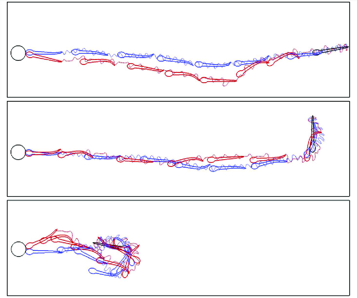
As introduced in § 3.1, the learned control policies of the FTP and VTP swimmers are fundamentally different from each other. For comparison, figure 5 shows the trailing-edge trajectories of the FTP and VTP swimmers, as well as their positions and gestures at several instants for three typical cases:  $(r_{tip,{0}},\theta _{tip,{0}})=(8L,0^\circ )$,
 $(8L,90^\circ )$ and
 $(3L,170^\circ )$. The full animation can be found in the supplementary material (movies 1, 2 and 3 available at https://doi.org/10.1017/jfm.2025.45). The whole swimming process is composed of two stages: first, turn fast to make the head face the target, then cruise nearly straight to the target. It is seen that the trajectories of swimmers with VTP and those with FTP are very close to each other, but the gestures are quite different. Characterized by the trailing-edge trajectory, an intermittent swimming style with burst-and-coast strategy is favoured by swimmers with VTP, which is widely observed in nature (Muller & Van Leeuwen Reference Müller and Van Leeuwen2004), while for swimmers with FTP, a continuous swimming style is developed.
Trailing-edge trajectories of swimmers with FTP and VTP, and their positions and gestures at several instants with three initial settings: (a)  $r_{tip,\textrm {0}}=8L$ and
 $\theta _{tip, \textrm {0}}=10^\circ$, (b)
 $r_{tip,\textrm {0}}=8L$ and
 $\theta _{tip, \textrm {0}}=90^\circ$, (c)
 $r_{tip,\textrm {0}}=3L$ and
 $\theta _{tip, \textrm {0}}=170^\circ$.

For a detailed illustration of swimming performance, figure 6 shows the time history of the lateral displacement of the tail tip  $y_{l,tail}$, the orientation angle
 $\theta _{tip}$, the swimming speed
 $u_r$ and the hydrodynamic power coefficient
 $C_P=PT^3/0.5\rho L^4$ for the case with
 $r_{tip,\textrm {0}}=8L$ and
 $\theta _{tip,\textrm {0}}=90^\circ$. It is noted that in FTP continuous swimming,
 $91$ tail flicks are used, which are regular and nearly symmetrical with slight adjustments. In VTP intermittent swimming, only
 $63$ tail flicks are used, and the tail-beat amplitude is highly asymmetrical with the period constantly changing, indicating that the fish is always adjusting its body kinematics during the swimming. However, a repeated pattern could still be observed in VTP intermittent swimming, in which the fish coasts for a short interval after every three tail flicks. Compared with continuous swimming, the variations of the swimming speed, orientation angle and hydrodynamic power are larger in intermittent swimming.
The temporal evolution of (a) lateral amplitude of the tail tip  $y_{l,tail}$, (b) orientation angle of the head
 $\theta _{tip}$, (c) swimming speed
 $u_r$, and (d) input work coefficient
 $C_P$, for the fish swimming system with
 $r_{tip,\textrm {0}}=8L$ and
 $\theta _{tip,\textrm {0}}=90^\circ$. A zoomed-in view of the area located between the green vertical lines in (a) will be presented in figure 9(a). Here,
 $T$ is the fixed characteristic time ensuring
 $Re=L^2/T\nu =1000$.

We also measured the time-averaged swimming performance over the entire swimming process for FTP and VTP swimmers within the parameter space, i.e.  $r_{tip,\textrm {0}}\in [3L, 9L]$ and
 $\theta _{tip,\textrm {0}}\in [0^\circ , 180^\circ ]$. Figure 7 shows contour plots for the time-averaged swimming speed
 $\bar {U}$, peak-to-peak amplitude of the tail tip
 $\bar {A}_{tail}$, swimming period
 $\bar {T}_a$ and cost of transport
 $COT$ as functions of initial distance
 $r_{tip,\textrm {0}}$ and oriented angle
 $\theta _{tip,\textrm {0}}$. Observation of figures 7(a) and 7(e) shows a high consistency in the time-averaged swimming speeds of FTP and VTP swimmers across the entire parameter space. Both speeds increase with
 $r_{tip,\textrm {0}}$ but decrease with
 $\theta _{tip,\textrm {0}}$. Figures 7(b) and 7(f) show that
 $\bar {A}_{tail}$ tends to rise with the initial oriented angle, peaking near the case with maximum
 $\theta _{tip,\textrm {0}}$ and minimum
 $r_{tip,\textrm {0}}$. It is because turning requires large body deformation, i.e. tail-beat amplitude, so a larger
 $\theta _{tip,\textrm {0}}$ leads to a larger
 $\bar {A}_{tail}$, while a small
 $r_{tip,\textrm {0}}$ requires a higher proportion of the total flicks for turning. This also explains the speed variation. Figures 7(c) and 7(g) indicate that
 $\bar {T}_a$ remains within a relatively stable and narrow range, without showing any apparent regular changes. The cost of transport is defined as
 $COT=\bar {C}_P/\bar {U}$, and
 $\bar {C}_P$ usually scales as
 $(f\bar {A}_{tail})^3$ (Lighthill Reference Lighthill1971), so the increase of
 $COT$ shows a similar trend with the decreasing of
 $\bar {U}$ and the increasing of
 $\bar {A}_{tail}$, as shown in figures 7(d) and 7(h). Finally, comparing the first and second rows of figure 7, VTP swimmers tend to use smaller peak-to-peak tail-beat amplitudes and longer swimming periods than FTP swimmers, resulting in lower energy consumption under similar
 $\bar {U}$ distributions.
Parameter space for (a–d) VTP intermittent swimming and (e–h) FTP continuous swimming. Contour plot of time-averaged (a,e) swimming speed ( $\bar {U}$), (b,f) peak-to-peak amplitude of tail tip (
 $\bar {A}_{tail}$), (c,g) swimming period (
 $\bar {T}_a$) and (d,h) cost of transport (
 $COT$) against initial distance (
 $r_{tip,\textrm {0}}$) and initial oriented angle (
 $\theta _{tip,\textrm {0}}$), where the unit of the vertical axis is degrees.

Comparison of swimming performance of VTP intermittent swimming and FTP continuous swimming. (a) Relative deviation in cost of transport ( $\triangle COT^*$) versus relative deviation in time-averaged swimming speed (
 $\triangle \bar {U}^*$). (b) Relative deviation in time-averaged peak-to-peak tail tip amplitude (
 $\triangle \bar {A}_{tail}^*$) versus relative deviation in swimming period (
 $\triangle \bar {T}_a^*$).

To quantitatively compare the swimming performance, we measure the relative differences of time-averaged peak-to-peak tail tip amplitude ( $\triangle \bar {A}_{tail}^*$), swimming period (
 $\triangle \bar {T}_a^*$), cost of transport (
 $\triangle COT^*$) and swimming speed (
 $\triangle \bar {U}^*$) between VTP intermittent swimming and FTP continuous swimming. These variables are defined as
 \begin{equation} \triangle \bar {A}_{tail}^*(r_{tip,\textrm {0}},\theta _{tip,\textrm {0}})=\frac {\bar {A}_{tail}^{VTP}(r_{tip,\textrm {0}},\theta _{tip,\textrm {0}})-\bar {A}_{tail}^{FTP}(r_{tip,\textrm {0}},\theta _{tip,\textrm {0}})}{\bar {A}_{tail}^{FTP}(r_{tip,\textrm {0}},\theta _{tip,\textrm {0}})}, \end{equation}
 \begin{equation} \triangle \bar {T}_a^*(r_{tip,\textrm {0}},\theta _{tip,\textrm {0}})=\frac {\bar {T}_a^{VTP}(r_{tip,\textrm {0}},\theta _{tip,\textrm {0}})-\bar {T}_a^{FTP}(r_{tip,\textrm {0}},\theta _{tip,\textrm {0}})}{\bar {T}_a^{FTP}(r_{tip,\textrm {0}},\theta _{tip,\textrm {0}})}, \end{equation}
 \begin{equation} \triangle \bar {U}^*(r_{tip,\textrm {0}},\theta _{tip,\textrm {0}})=\frac {\bar {U}^{VTP}(r_{tip,\textrm {0}},\theta _{tip,\textrm {0}})-\bar {U}^{FTP}(r_{tip,\textrm {0}},\theta _{tip,\textrm {0}})}{\bar {U}^{FTP}(r_{tip,\textrm {0}},\theta _{tip,\textrm {0}})}, \end{equation}
 \begin{equation} \triangle COT^*(r_{tip,\textrm {0}},\theta _{tip,\textrm {0}})=\frac {COT^{VTP}(r_{tip,\textrm {0}},\theta _{tip,\textrm {0}})-COT^{FTP}(r_{tip,\textrm {0}},\theta _{tip,\textrm {0}})}{COT^{FTP}(r_{tip,\textrm {0}},\theta _{tip,\textrm {0}})}, \end{equation}
where the superscripts  $VTP$ and
 $FTP$ represent the VTP intermittent swimming and FTP continuous swimming, respectively. To ensure comparability, we strive to match the mean speeds of FTP swimming and VTP swimming as closely as possible. Figure 8(a) shows speed deviation (
 $\triangle \bar {U}^*$) within
 $5\, \%$ for all cases, mostly under
 $2.5\, \%$, confirming comparability. We can also see from figure 8 that the majority of data points within the parameter space occupy the region specified by
 $\triangle COT^*\lt 0$ (constituting
 $85.4\, \%$ of the data),
 $\triangle \bar {A}_{tail}^*\lt 0$ (accounting for
 $93.9\, \%$ of the total), and
 $\triangle \bar {T}_a^*\gt 0$ (representing
 $97.6\, \%$ of the total). The average values of
 $\triangle COT^*$,
 $\triangle \bar {A}_{tail}^*$ and
 $\triangle \bar {T}_a^*$ in all cases are
 $-15.2\, \%$,
 $-14.1\, \%$ and
 $12.1\, \%$, respectively. Despite not always outperforming continuous swimming in energy efficiency, VTP intermittent swimming tends to adopt a lower flapping amplitude and a higher flapping period to achieve a minimized cost of transport compared to FTP continuous swimming.
The temporal evolution of (a) lateral position of the tail tip  $y_{l,tail}$, (b) swimming speed
 $u_r$, (c) force coefficient in the
 $x_l$-direction
 $C_F$, and (d) input power coefficient
 $C_P$, for the fish swimming system with
 $r_{tip,\textrm {0}}=8L$ and
 $\theta _{tip,\textrm {0}}=90^\circ$ in a short period (the time period is identified by the two green dashed lines in figure 6a). The FTP continuous swimming and VTP intermittent swimming are marked by blue dashed lines and red solid lines, respectively. In (a), black circles and green squares denote special moments from figures 10 and 11, respectively.

3.3. Hydrodynamics
To enhance our understanding of the propulsive performance of intermittent swimming, the time history of the lateral tail movement, the swimming speed, the orientation angle and the hydrodynamic power in a specific burst-and-coast cycle are analysed in detail and compared with continuous swimming, as shown in figure 9. Notably, figure 9, as well as the subsequent figures 10 and 11, showcasing the swimming performance and vorticity field of the case with  $(r_{tip, \textrm {0}}, \theta _{tip, \textrm {0}})=(8L, 90^\circ )$ over a specific time period, serve as representative samples to reflect the primary swimming performances of VTP intermittent and FTP continuous swimming. It is seen that a full burst-and-coast cycle is composed of three tail flicks and a coast phase. Ashraf et al. (Reference Ashraf, Van Wassenbergh and Verma2020) observed similar temporal evolution of the lateral position of the tail tip in another species (Hemigrammus bleheri), despite variations in the cruising Reynolds number. Flick 1 is a preparatory flick, in which the tail moves slowly to the left side of the body from a straight posture (the duration of the flick is approximately
 $0.7T$). This flick leads to an immediate change of the orientation angle from approximately
 $-6^\circ$ to
 $5^\circ$ (turning left; figure not shown). However, the influence on the swimming speed is much smaller as it continuously decreases as in the coast phase, and the hydrodynamic power remains at a low level. After that, the fish initiates a strong flick (flick 2 in figure 9), which flaps from left to right within a duration of only approximately
 $0.3T$. The strong flick leads to an intense increase in the swimming speed, thrust and the hydrodynamic power, and recovers the orientation angle from
 $5^\circ$ to
 $-4^\circ$. In flick 3, the fish recovers to the straight posture and then coasts for duration
 $0.5T$. In the last flick and the coast phase, the swimming speed is continuously decreasing, and the change of the orientation angle is negligible. Compared with intermittent swimming, continuous motion shows more continuous changes and lower oscillations in swimming speed, force and energy performance.
To delve into the hydrodynamics of continuous and intermittent swimming, the instantaneous vorticity contour and distribution of crucial physical variables, including velocity ( ${\boldsymbol{u}}_B=\partial {\boldsymbol{X}}/\partial t$), hydrodynamic force (
 ${\boldsymbol{F}}_f$) and power (
 $P_B=-{\boldsymbol{F}}_f\boldsymbol{\cdot} (\partial {\boldsymbol{X}}/\partial t)$), on the body surface during both swimming modes are depicted in figures 10 and 11. A comprehensive animation is available in supplementary movies 4 and 5. The continuous swimming is highly periodic, with the tail alternatively flapping leftwards and rightwards. In each flick, a vortex is generated due to the lateral flapping motion around the tail tip, which induces strong lateral force, lateral flow and energy consumption near the tail. Those vortices are organized in a straight line, forming a typical zero-thrust wake.
The instantaneous vorticity contour, and distribution of key physical variables on the body surface:  $1$ velocity
 ${\boldsymbol{u}}_B$ (the red arrow represents the velocity vector);
 $2$ hydrodynamic force
 ${\boldsymbol{F}}_f$ (the blue arrow represents the hydrodynamic force distribution on the body);
 $3$ input power
 $P_B$, for the FTP continuous swimmer at (a)
 $t=25.6$, (b)
 $t=25.8$, (c)
 $t=26.0$ and (d)
 $t=26.3$. The lateral amplitudes of the tail tip for these special moments are marked by black circles in figure 9(a).

The instantaneous vorticity contour, and distribution of key physical variables on the body surface:  $1$ velocity
 ${\boldsymbol{u}}_B$ (the red arrow represents the velocity vector);
 $2$ hydrodynamic force
 ${\boldsymbol{F}}_f$ (the blue arrow represents the hydrodynamic force distribution on the body);
 $3$ input power
 $P_B$, for the VTP swimmer at (a)
 $t=25.7$, (b)
 $t=26.4$, (c)
 $t=26.5$, (d)
 $t=26.6$, (e)
 $t=26.8$ and (f)
 $t=27.1$. The lateral amplitudes of the tail tip for these special moments are marked by green squares in figure 9(a).

For intermittent swimming, from instant  $t/T=25.7$ to
 $t/T=26.4$ (figures 11a,b), the fish flaps its tail leftwards and forwards from a straight posture (flick 1). Meantime, an anticlockwise vortex (vortex 1) is generated and shed into the wake flow. Since the fish is pushing the ambient fluid forwards, it mainly experiences a net drag on the body and decelerates continuously (except for the time interval
 $t/T\in [26.3, 26.4]$). From instant
 $t/T=26.4$ to
 $t/T=26.7$ (figures 11b–d), the fish flaps its tail rightwards and backwards with a strong flick (flick 2). The tail movement induces strong backward flow around the posterior part (seen obviously in figure 11c). Meantime, a strong clockwise vortex (vortex 2) forms and detaches at the tail tip, creating a low-pressure region that generates suction ahead of the fish’s posterior part as it moves. Moreover, as the fish pushes the ambient fluid backwards, it experiences a strong thrust and energy consumption on the posterior part, and accelerates continuously. From instant
 $t/T=26.7$ to
 $t/T=27.1$ (figures 11d,e), the fish flaps its tail from the right-hand side to the balanced point (flick 3), releasing the attached vortex from the posterior part into the wake flow, and generating another anticlockwise vortex (vortex 3). The vortex is close to vortex 2, forming a vortex pair. It should be noted that the vortex pair in the wake flow is also found in several experiments and numerical simulations (Muller et al. Reference Müller, Stamhuis and Videler2000; Wu et al. Reference Wu, Yang and Zeng2007; Floryan et al. Reference Floryan, Van Buren and Smits2017; Dai et al. Reference Dai, He, Zhang and Zhang2018; Akoz et al. Reference Akoz, Mivehchi and Moored2021; Gupta et al. Reference Gupta, Thekkethil, Agrawal, Hourigan, Thompson and Sharma2021). From instant
 $t/T=27.1$ to
 $t/T=27.5$ (figure 11f), the fish is in the coast phase and there is no new vortex generated. It is noteworthy that although vortex 3 formed in flick 3 and pairs with vortex 2 to form a pair of reverse Kármán vortex streets, vortex 3’s proximity to the deformed posterior of the fish exerts a more immediate influence. This results in the creation of a suction zone behind the posterior, which subsequently leads to drag. Moreover, during the coast phase, because the body is already in a straight state, the vortex pair does not contribute significantly to thrust. In the whole coast phase, the fish decelerates continuously as shown in figure 9(b). We note that the coast phase is superior to the forward flicks (flicks 1 and 3) in energy efficiency (as shown in figure 9d), since those flicks are consuming energy to produce drag. In this regard, flicks 1 and 3 are more like ‘in-between flicks’ to connect the powerful thrust-generating flick 2 and the energy-saving coast phase.
3.4. Scaling laws
To systematically enhance our understanding of the swimming performance of fish trained to expend minimal energy, we delve into the scaling laws of FTP and VTP swimmers. Specifically, we investigate the relationship between swimming speed  $\bar {U}$ and body kinematics, encompassing the time-averaged peak-to-peak tail tip amplitude
 $\bar {A}_{tail}$, swimming period
 $\bar {T}_a$ and duty cycle
 $DC$, as well as fluid properties (kinematic viscosity
 $\nu$). In this subsection, we set the initial orientation angle to zero, thereby minimizing or eliminating turning, and ensuring that the fish in training remain in a cruising state. The initial position
 $r_{tip,0}$ ranges from
 $3L$ to
 $9L$ with interval
 $0.5L$. To obtain a wider range of cruising Reynolds number, we set several different sets of mean swimming period (
 $T_m$), with
 $T_{m}$ ranging from
 $0.6T$ to
 $1.4T$ with interval
 $0.2T$. For each set, the tail-beat period (two tail flicks) of the FTP swimmer is fixed at
 $T_a=T_{m}$, while for the VTP swimmer, the selectable tail-beat periods are
 $T_a=T_{m}-0.4$,
 $T_m-0.2$,
 $T_{m}$,
 $T_{m}+0.2$,
 $T_m+0.4$. The tail-beat amplitude of each tail flick can be chosen from
 $\theta _{lmax}=0^\circ , 10^\circ , 20^\circ , 30^\circ , 40^\circ , 50^\circ , 60^\circ , 70^\circ , 80^\circ , 90^\circ , 100^\circ , 110^\circ, 120^\circ$.
Inspired by previous works (Gazzola et al. Reference Gazzola, Argentina and Mahadevan2014a; van Leeuwen et al. Reference van Leeuwen, Voesenek and Müller2015; Liu et al. Reference Liu, Liu and Huang2022; Kang et al. Reference Kang, Gong, Lu, Cui and Fan2023), we introduce three key non-dimensional parameters: the swimming number  $Sw$ (i.e. the flapping Reynolds number in the study of Liu et al. (Reference Liu, Liu and Huang2022) and Kang et al. (Reference Kang, Gong, Lu, Cui and Fan2023)), the cruising Reynolds number
 $Re_u$, and the duty cycle
 $DC$, which are defined as
 \begin{equation} Sw=2\pi f\bar {A}_{tail}L/\nu ,\ \ Re_u=\bar {U}L/\nu , \ \ DC=T_b/T_{cyc}, \end{equation}
where  $f=1/\bar {T}_a$ is the flapping frequency,
 $\bar {A}_{tail}$ is the time-averaged peak-to-peak amplitude of the tail tip, and
 $\bar {U}$ is the mean swimming speed during cruising swimming. The duty cycle
 $DC$ serves to quantify the fraction of active motion time (
 $T_b$) within a complete flapping cycle (
 $T_{cyc}$), where
 $T_{cyc}$ comprises the sum of burst phase duration (
 $T_b$) and coast phase duration (
 $T_c$). For continuous swimming,
 $T_b=T_{cyc}$ and
 $DC=1$. Taking the example of an intermittent flapping cycle marked with flicks 1, 2, 3 and coast in figure 9, which includes four flicks, and noting that
 $T_{flick1}$,
 $T_{flick2}$,
 $T_{flick3}$ and
 $T_{flick,coast}$ represent the durations of flicks 1, 2, 3 and the coast phase, respectively, the burst phase duration
 $T_b$ during this cycle is
 $T_{flick1}+T_{flick2}+T_{flick3}$, and the duration of a complete flapping cycle
 $T_{cyc}$ is
 $T_{flick1}+T_{flick2}+T_{flick3}+T_{flick,coast}$. Since a VTP swimmer can alter its tail-beat frequency every flick, the duty cycle (
 $DC$) of each burst-and-coast action varies. Hence in this work,
 $DC$ is estimated as the ratio of the total active flick (or burst) duration to the entire cruising duration.
Schematic diagram for (a) force decomposition and (b) thrust and drag contribution from pressure force and viscous force. Here,  $\boldsymbol {n}$ and
 $\boldsymbol {\tau}$ represent the local normal and tangential vectors, respectively,
 ${\boldsymbol{F}}_{f,i}$ signifies the hydrodynamic force, and
 ${\boldsymbol{F}}_i^n=(F_{x,i}^n, F_{y,i}^n)$ and
 ${\boldsymbol{F}}_i^{\tau }=(F_{x,i}^\tau , F_{y,i}^\tau )$ represent pressure force and viscous force acting on the
 $i$th surface element of the fish body. (c,d) The
 $x$-component of the hydrodynamic force
 $F_x={\boldsymbol{F}}_f\boldsymbol{\cdot} {\boldsymbol {e}}_x$, thrust
 $F_T$, and drag
 $F_D$ as functions of time for (c) FTP swimming and (d) VTP swimming. Here,
 ${\boldsymbol {e}}_x$ denotes the unit vector aligned with the
 $x$-axis.

The swimming performance of the fish hinges on both the hydrodynamic force acting on its body surface and the deformation of its body. As depicted in figure 12(a), the hydrodynamic force  ${\boldsymbol{F}}_f$ exerted on the body is composed of the pressure-dominated normal force
 ${\boldsymbol{F}}^n$ and the tangential force stemming from viscous effects
 ${\boldsymbol{F}}^\tau $, i.e.
 ${\boldsymbol{F}}_f={\boldsymbol{F}}^n+{\boldsymbol{F}}^\tau$. The specific definitions of these forces at the
 $i$th surface element are (Liu et al. Reference Liu, Liu and Huang2022)
 \begin{equation} {\boldsymbol{F}}_{f,i}=(-p\mathbf {I}+\mathbf {T})\boldsymbol{\cdot} {\boldsymbol {n}}={\boldsymbol{F}}_i^n+{\boldsymbol{F}}_i^\tau , \end{equation}
 \begin{equation} {\boldsymbol{F}}_i^n=({\boldsymbol{F}}_i\boldsymbol{\cdot} {\boldsymbol {n}})\boldsymbol{\cdot} {\boldsymbol {n}}=\big(F_{x,i}^n, F_{y,i}^n\big), \end{equation}
 \begin{equation} {\boldsymbol{F}}_i^\tau =({\boldsymbol{F}}_i\boldsymbol{\cdot} {\boldsymbol {t}})\boldsymbol{\cdot} {\boldsymbol {t}}=\big(F_{x,i}^\tau , F_{y,i}^\tau \big), \end{equation}
where  $\mathbf {I}$ and
 $\mathbf {T}$ represent the unit tensor and viscous stress tensor, respectively, and
 $\boldsymbol {n}$ and
 $\boldsymbol {t}$ are the unit normal vector and unit tangential vector on the body surface, respectively. As illustrated in figure 12(b), the pressure force
 ${\boldsymbol{F}}_i^n$ can contribute to either thrust or drag, and similarly the tangential force
 ${\boldsymbol{F}}_i^\tau$ may also contribute to either thrust or drag, which depends on the local fluid–structure interaction occurring near the
 $i$th body surface element. Here, the thrust
 $F_T$ and drag
 $F_D$ can be defined precisely through a force decomposition analysis (Bottom et al. Reference Bottom II, Borazjani, Blevins and Lauder2016):
 \begin{eqnarray} -F_T(t)&=\tfrac {1}{2}(F_x^n-|F_x^n|)+\tfrac {1}{2}(F_x^\tau -|F_x^\tau |), \end{eqnarray}
 \begin{eqnarray} F_D(t)&=\tfrac {1}{2}(F_x^n+|F_x^n|)+\tfrac {1}{2}(F_x^\tau +|F_x^\tau |). \end{eqnarray}
It is noted that the fish is swimming in the  $-x$ direction. The time-averaged thrust and drag are defined as
 $\bar {F}_T=(1/T_{tot})\int _{t^{\prime}}^{t^{\prime}+T_{tot}}F_T(t)\,{\rm d}t$ and
 $\bar {F}_D=(1/T_{tot})\int _{t^{\prime}}^{t^{\prime}+T_{tot}}F_D(t)\,{\rm d}t$, respectively, where
 $t'$ and
 $T_{tot}$ are the start time and the time range during which the fish maintains its cruising state. Figures 12(c) and 12(d) illustrate the thrust and drag profiles for FTP continuous swimming and VTP intermittent swimming, respectively. For continuous swimming, the drag and thrust persist throughout the entire motion process, with the drag exhibiting relatively minor variations in magnitude compared to the thrust. In contrast, for intermittent swimming, thrust is concentrated primarily in the burst phase, exemplified by flicks 1, 2 and 3 in figure 9. Specifically, the rapid backstroke of flick 2 generates a significant thrust. Drag, on the other hand, persists throughout the entire motion process, with its value during the active burst phase being notably higher than that during the passive coasting phase.
We conduct an investigation into the scaling relation between key non-dimensional parameters for both continuous and intermittent swimming. The underlying thrust–drag balance during cruising provides valuable insights into interpreting these scaling laws. By the elongated-body theory (Lighthill Reference Lighthill1971), the thrust scaling for active swimming (continuous swimming or burst phase) is  $\bar {F}_T\sim (f\bar {A}_{tail})^2$, which is identical to that in previous studies (e.g. Gazzola et al. Reference Gazzola, Argentina and Mahadevan2014a; Quinn et al. Reference Quinn, Moored, Dewey and Smits2014; Liu et al. Reference Liu, Liu and Huang2022; Kang et al. Reference Kang, Gong, Lu, Cui and Fan2023). For the laminar boundary layer, the drag is dominated by viscous drag and scales as
 $\bar {U}^{1.5}$, whereas for the turbulent boundary layer, the drag is dominated by pressure drag and scales as
 $\bar {U}^2$ (Gazzola et al. Reference Gazzola, Argentina and Mahadevan2014a). The swimming in the present study is in the intermediate Reynolds regime, so the drag scales as
 $\bar {F}_D\sim \bar {U}^{3/2}$. The previous experimental data (Lighthill Reference Lighthill1971; Webb Reference Webb1971) suggest that the drag of actively swimming fish is increased over the value for a rigid body by a factor of 3–5. Here, we set
 $\beta$ as the ratio of drag coefficients between active swimming and passive coasting, which is greater than 1. Balancing the thrust and drag, Kang et al. (Reference Kang, Gong, Lu, Cui and Fan2023) derived the scaling laws for the key parameters, i.e.
 \begin{equation} \bar {F}_T\sim Sw^2/DC\sim \big(Sw/\sqrt {DC}\big)^2, \end{equation}
 \begin{equation} \bar {F}_D\sim [(\beta -1)DC+1]Re_u^{1.5}\sim \{Re_u[(\beta -1)DC+1]^{2/3}\}^{3/2}, \end{equation}
 \begin{equation} Re_u^{1.5}\sim Sw^2/\big[(\beta -1)DC^2+DC\big]\sim \big[Sw/\sqrt {(\beta -1)DC^2+DC}\big]^2. \end{equation}
Following the elongated-body theory (Lighthill Reference Lighthill1971), it is easy to derive that the input power scales as  $\bar {P}\sim Sw^3/DC^2$, which is confirmed by previous studies, i.e. Kang et al. (Reference Kang, Gong, Lu, Cui and Fan2023), and the cost of transport (
 $COT=\bar {P}/m\bar {U}$) can be scaled as
 \begin{equation} COT\sim Sw^{5/3}[(\beta -1)/DC+1/DC^2]^{2/3}\sim \{Sw[(\beta -1)/DC+1/DC^2]^{2/5}\}^{5/3}. \end{equation}
Scaling swimming performance for swimmers with FTP (black circles) and VTP (red squares). The cruising Reynolds number  $Re_u$ is a function of
 $Sw^*=Sw/\sqrt {(\beta -1)DC^2+DC}$, and
 $\beta =2.5$.

The cruising Reynolds number  $Re_u$ as a function of
 $Sw^*=Sw/\sqrt {(\beta -1)DC^2+DC}$ is depicted in figure 13. It is seen that for both FTP swimmers and VTP swimmers,
 $Re_u$ values of all cases follow the same scaling law approximately, i.e.
 $Re_u\sim Sw^{* 4/3}$. It is identical to that in Gazzola et al. (Reference Gazzola, Argentina and Mahadevan2014a)for continuous swimming, i.e.
 $Re_u\sim Sw^{4/3}$. For intermittent swimming, the result is also consistent with the numerical finding of Kang et al. (Reference Kang, Lu and Cui2022), although the
 $\beta$ values are different (
 $\beta =2.5$ in the present work, whereas
 $\beta =3$ and
 $1$ for pitching and heaving flexible plates, respectively, in Kang et al. Reference Kang, Lu and Cui2022).
Scaling swimming performance for swimmers with FTP (black circles) and VTP (red squares). (a) The thrust  $\bar {F}_T$ as a function of the modified swimming number
 $Sw'=Sw/DC^{0.5}$. (b) The drag
 $\bar {F}_D$ as a function of the modified Reynolds number
 $Re'_{\!\!u}=Re_u/[(\beta -1)DC+1]^{2/3}$. Here,
 $\beta =2.5$.

Next, the scaling laws for thrust  $\bar {F}_T$ and drag
 $\bar {F}_D$ are discussed. Figure 14 plots the thrust
 $\bar {F}_T$ versus the modified swimming number
 $Sw'=Sw/DC^{0.5}$, and the drag
 $\bar {F}_D$ versus the modified Reynolds number
 $Re'_{\!\!u}=Re_u/[(\beta -1)DC+1]^{2/3}$. It is seen that
 $\bar {F}_T$ is proportional to
 $Sw'$, and
 $\bar {F}_D$ is proportional to
 $Re'_{\!\!u}$. The numerical results align well with the theoretical scaling laws. Furthermore, it is observed that the FTP data sets converge neatly into a single curve, while the VTP data sets exhibit a more disperse pattern. This discrepancy could potentially be attributed to the fact that the flapping amplitude, period and duty cycle of the trained fish are not fixed during each swimming cycle, making the time-averaged value a mere approximation of their swimming performance. Analogous phenomena are also observed in other scale-law analyses pertaining to biological data, including Gazzola et al. (Reference Gazzola, Argentina and Mahadevan2014a) and van Leeuwen et al. (Reference van Leeuwen, Voesenek and Müller2015).
Finally, the cost of transport is considered, as presented in figure 15. It is seen that the cost of transport  $COT$ can be scaled as
 $COT\sim Sw^{\circ \ 5/3}$ for both FTP swimming and VTP swimming, where
 $Sw^{\circ }=Sw*[(\beta -1)/DC+1/DC^2]^{2/5}$. It is also consistent with our theoretical scaling law.
Scaling swimming performance for swimmers with FTP (black circles) and VTP (red squares). Cost of transport  $COT$ is a function of
 $Sw^{\circ }=Sw*[(\beta -1)/DC+1/DC^2]^{2/5}$, and
 $\beta =2.5$.

4. Conclusion
The point-to-point navigation of a larval-zebrafish-like swimmer is studied numerically with a hybrid method of deep reinforcement learning and the immersed boundary–lattice Boltzmann method. The goal of the swimmer is to reach its target with minimized energy expenditure. Specifically, two situations are investigated, in which the swimmer is swimming with fixed tail-beat period and variable tail-beat period. When swimming in fixed period, the optimized strategy is to swim in a continuous pattern, in which the tail beat is regular and nearly symmetrical. When swimming in variable period, the optimized strategy is to swim in an intermittent pattern, in which the tail beat is highly asymmetrical and time-varying. Compared with continuous swimming, intermittent swimming displays a greater variation in swimming speed, orientation angle and hydrodynamic power, while generally exhibiting lower mean tail-beat amplitude, frequency and energy expenditure. Specifically, the mean tail-beat period of intermittent swimming is approximately  $12.1\, \%$ longer than that of continuous swimming (average across all cases), while the mean tail-beat amplitude and cost of transportation are, respectively,
 $14.1\, \%$ and
 $15.2\, \%$ lower. A detailed investigation shows that a full burst-and-coast cycle is composed of four phases: a powerful thrust-generating flick to accelerate and maintain the swimming speed, a totally passive coast phase to save energy, and two in-between tail flicks to ensure a smooth transition between the thrust-generating and energy-saving phases. The swimming performance can be summarized as some scaling laws: specifically, the cruising Reynolds number
 $Re_u$ scales as
 $Re_u\sim [Sw/\sqrt {(\beta -1)DC^2+DC} ]^{4/3}$, while the thrust
 $\bar {F}_T$ and drag
 $\bar {F}_D$ scale as
 $\bar {F}_T\sim (Sw/\sqrt {DC} )^2$ and
 $\bar {F}_D\sim \{Re_u[(\beta -1)DC+1]^{2/3}\}^{3/2}$, respectively. Additionally, the cost of transport follows the scaling
 $COT\sim \left \{Sw[(\beta -1)/DC+1/DC^2]^{2/5}\right \}^{5/3}$. This study holds promise in deepening our understanding of aquatic animal locomotion and significantly contributing to bionic design.
In the present study, the discussion of energy-optimized swimming is restricted to individual swimmers. It is, however, noteworthy that various species of fish adopt collective intermittent swimming as an energy-efficiency locomotion mode (Wang et al. Reference Wang, Escobedo, Sanchez, Han, Sire and Theraulaz2024a). While the swimming performance of multiple fish/fins utilizing intermittent swimming in various formations (Kang et al. Reference Kang, Lu and Cui2022; Jeong et al. Reference Jeong, Kim and Lee2023) has been studied in detail, there is a potential trade-off between enhancing group cohesion and optimizing individual energy efficiency for real aquatic animals (Noda et al. Reference Noda, Fujioka, Fukuda, Mitamura, Ichikawa and Arai2016). In light of this, considering various influencing factors and the freedom of movement, applying reinforcement learning to the collective motion of multiple individuals emerges as a highly valuable research topic. Further, while the present scaling laws have been supported by the training data, due to the limitation of currently available biological observation (Gazzola et al. Reference Gazzola, Argentina and Mahadevan2014a; van Leeuwen et al. Reference van Leeuwen, Voesenek and Müller2015), particularly description of swimming intermittency, direct validation from biological data is currently unattainable. To validate and refine our model, we require more comprehensive biological data. This will establish a theoretical basis for comparing training and biological data, allowing us to investigate if minimizing energy is the main objective of fish swimming.
Supplementary movies
Supplementary movies are available at https://doi.org/10.1017/jfm.2025.45.
Funding
The authors acknowledge the support provided by the National Natural Science Foundation of China (grant nos 12102365,12302365), National Key Research and Development Program of China (grant no. 2022YFC2805200), the Australian Research Council (grant no. DE160101098), Human Frontier Science Program (RGY0059/2022), Research Center for Industries of the Future at Westlake University (WU2022C036), and Key Research and Development Program of Zhejiang Province (2023C03133).
Declaration of interests.
The authors report no conflict of interest.



