Nomenclature
-
 $ Oxyz $
-
transport inertial coordinate systems
-
$O{x_I}{y_I}{z_I}$
-
launch inertial coordinate systems
-
$O{x_s}{y_s}{z_s}$
-
inertial line-of-sight (LOS) coordinate systems
-
${q_\varepsilon }$
-
line of sight elevation
$\left({^ \circ } \right)$
-
${q_\beta }$
-
line of sight azimuth
$\left({^ \circ } \right)$
-
${x_m}$
-
interceptor position vector in inertial LOS coordinate systems
$\left( m \right)$
-
${V_m}$
-
interceptor velocity vector in inertial LOS coordinate systems
$\left({m/s} \right)$
-
${{\bf{U}}_m}$
-
interceptor acceleration vector in inertial LOS coordinate systems
$\left({m/{s^2}} \right)$
-
${t_e}$
-
predicted time of hit
-
${{\bf{p}}_m}$
-
interceptor zero control terminal position
$\left( m \right)$
-
$M\!\left(t\right)$
-
interceptor interceptable area
-
${X_T}$
-
target state vector in inertial coordinate systems
$\left({m/s} \right)$
-
${{\bf{U}}_T}$
-
target acceleration vector in inertial coordinate systems
$\left({m/{s^2}} \right)$
-
${X_T}\left({{t_0}} \right)$
-
mean matrix of the initial moment motion state
-
${Q_{{X_T}}}\left({{t_0}} \right)$
-
covariance matrix of the initial moment motion state
-
${U_{{T_0}}}$
-
mean of the control inputs
-
$R$
-
target predicted manoeuvering escape zone
-
$\tilde R$
-
approximation of target predicted manoeuvering escape zone
-
${\Phi _m}\left({{t_e},{t_0}} \right)$
-
state transfer matrix for the interceptor motion model
-
${\Phi _T}\left({{t_e},{t_0}} \right)$
-
state transfer matrix for the target motion model


Greek symbol
-
$\xi $
-
point in the target manoeuvering escape region
-
$\sigma _{uT}^2$
-
variance of the control inputs


1.0 Introduction
In recent years, significant advancements have been made in space defense technologies. However, the intelligence [Reference Wang, He, Wang, Zhang, Yao and Chen1, Reference He, Wang, Ma and Zhang2] and manoeuverability of targets have also been continuously enhanced. Hypersonic vehicles, in particular, combine the high-speed characteristics of ballistic missiles with the high manoeuverability of cruise missiles, while exhibiting superior stealth and penetration capabilities [Reference Su, Shin, Chen and Tsourdos3]. These attributes pose substantial challenges to aerospace defense operations, rendering the interception of highly manoeuverable targets both a critical research focus and a technical bottleneck.
Given the superior speed and manoeuverability of such targets, interceptors often lack competitive advantages in these domains. Consequently, single-interceptor systems struggle to achieve effective interception, prompting multi-interceptor cooperative strategies to emerge as a prominent research area in recent years [Reference Jeon, Lee and Tahk4–Reference Shaferman and Oshman6]. Under modern complex battlefield conditions, however, early-warning systems frequently fail to obtain precise kinematic data of high-manoeuverability targets due to detection inaccuracies. Instead, only probabilistic target engagement zones can be estimated. Furthermore, each interceptor’s operational coverage remains limited. To ensure that the interception zones of multiple interceptors comprehensively or nearly fully encompass the target’s probable engagement area, the development of efficient area coverage optimisation methodologies has become imperative.
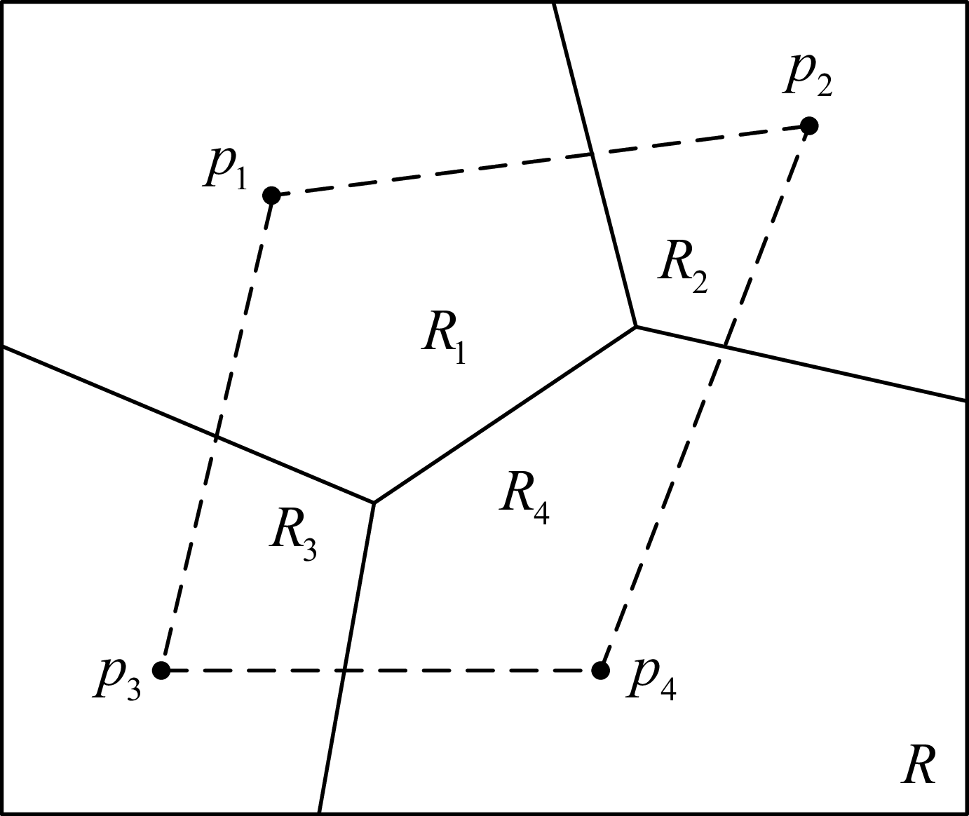
The Voronoi tessellation diagram of the area coverage problem is shown in Fig. 1.The optimisation of area coverage primarily addresses the deployment problem of interceptors [Reference Wang, Liu, Yao and He7], wherein each interceptor moves to an optimal position based on a corresponding algorithm and ultimately remains at that position to achieve optimal sensing and coverage of a given mission area. Representative area coverage optimisation methods can be categorised into three main types: geometry-based coverage methods [Reference Shu, Dsouza, Bhargava and de Silva8–Reference Ziyan, Jianglong, Xiwang and Zhang12], virtual force-based coverage methods [Reference Zeng, Xie, Wei, Chen and Wu13, Reference Wang, Yang, Wang and Qian14] and intelligence-based coverage methods [Reference Wang, Yao, He and Liu19–Reference Zhai, He, Hong, Wang and Yao22].
Description of the area coverage problem.

In geometry-based coverage methods, the Voronoi diagram is a widely utilised tool in computer graphics. Voronoi partitioning is a distance-based plane division method, where each sub-region contains points that are closer to the agent within that region than to any other agent. After partitioning the mission area, each agent moves toward the centroid of its corresponding sub-region. In Ref. (8), a GCVD (geometric centre Voronoi diagram) coverage method was proposed based on Voronoi diagrams (VD) and geometric centres (GC). This method ensures node-to-node connectivity while achieving maximum area coverage and minimal energy consumption for movement. Reference [Reference Gou, Guo, Guo and Mao9] addressed heterogeneous wireless sensor networks by introducing a VKECE-3D (Voronoi K-means energy-efficient coverage enhancement) method, which combines 3D-Voronoi partitioning and the K-means algorithm. This approach enhances network coverage and extends the network’s operational lifespan. Additionally, Refs. [Reference Liu, Yan, Zhang, Zhang and Yan11] and [Reference Ziyan, Jianglong, Xiwang and Zhang12] approximate both the target engagement zone and the interceptor’s coverage zone as circles. By applying the geometric principle of ‘small circles covering a large circle’, they achieve area coverage and design algorithms to quickly determine the minimum number of small circles and their centre positions, which represent the virtual target points for interceptors.
The virtual force algorithm (VFA) is a real-time obstacle avoidance algorithm for mobile robots that integrates the principles of artificial potential fields and grid-based methods. In Ref. [Reference Zeng, Xie, Wei, Chen and Wu13], VFA was combined with the Lloyd-Voronoi algorithm, reducing systems redundancy and enhancing the overall area coverage of the systems. Reference [Reference Wang, Yang, Wang and Qian14] introduced VFA into an embedded grey wolf optimisation (GWO) algorithm, achieving improved optimisation effects on sensor node coverage, uniformity and average movement distance.
Since area coverage optimisation inherently falls under the category of optimisation problems, various intelligent algorithms have gradually been applied to address such challenges. Reference [Reference Garber15] derives a closed-form optimal interception guidance law for accelerating targets. Reference [Reference Xiao, Wang, Zhang and Cheng16] proposed a distributed multi-agent dynamic area coverage algorithm based on reinforcement learning to obtain the global optimal or local optimal dynamic coverage strategy for the entire coverage process. Reference [Reference Mou, Zhang, Gao, Wang, Zhang and Han17] proposed a swarm deep Q-learning (SDQN) reinforcement learning algorithm based on the fast coverage problem of 3D irregular terrain surfaces with a hierarchical unmanned aerial vehicle (UAV) swarm. Reference [Reference Xin, Wang and Li18] considers the cooperative multi-area coverage problem using multiple robots in the presence of obstacles, points out the problems of high redundancy and poor scalability of existing algorithms and designed a genetic algorithm based on cyclic coding for area allocation.
In the context of cooperative interception of highly manoeuverable targets, the design of cooperative interception strategies and cooperative guidance laws represents a key research direction. Reference [Reference Wang, Yao, He and Liu19] addresses the problem of multi-interceptor cooperative interception with uncertain target information during mid-course guidance, proposing a stochastic optimisation problem to design the optimal relative motion parameters between the flight vehicle and target at the handover moment, ensuring interception probability with fewer interceptors and optimising interception strategies. Subsequently, in Ref. [Reference Long, Yu, Fenghua and Kai20], an algorithm based on Monte Carlo sampling and stochastic approximation for the optimisation problem mentioned above was proposed, which effectively solves the stochastic optimisation problem where random variables depend on the states to be optimised. Reference [Reference Su, Li and Chen21], based on coverage theory and bias proportional guidance law, derives the minimum relative manoeuverability advantage and formation size required to cover the entire target manoeuvering range, and designs cooperative guidance strategies for intercepting highly manoeuverable targets based on the presence or absence of communication capabilities in the formation. Reference [Reference Zhai, He, Hong, Wang and Yao22] combines coverage theory-based guidance laws with optimal control laws to achieve cooperative interception of targets with decoys.
In summary, virtual force-based coverage methods exhibit rapid convergence when solving coverage problems, but their optimisation effectiveness requires further improvement. Although intelligence-based coverage methods offer global search advantages, they exhibit high computational complexity, are prone to local optima, and demonstrate unstable convergence when applied to large-scale area coverage. Furthermore, the black-box nature of these algorithms undermines their interpretability and verifiability, posing potential risks in scenarios requiring stringent guarantees of coverage reliability. Therefore, this paper proposes a fast computation method for cooperative interception zones targeting highly manoeuverable threats, based on disk covering theory [Reference Weisstein23]. The main merits of this paper are concluded as follows:
-
1. Based on the equations of motion for both the interceptor and the target, approximate expressions for the interceptor interceptable region and the target escape region are derived.
-
2. A novel area-coverage algorithm based on disk covering theory is proposed.
Experimental validation demonstrates that the proposed method achieves excellent coverage of the predicted escape zone of the target while satisfying real-time requirements.
The remainder of this paper is organised as follows: Section 2 gives the problem formulation and preliminaries. In Section 3, the fast computation algorithm of cooperative interception zones for multiple aircraft is given. In Section 4, simulation results illustrate the effectiveness of the proposed algorithm. Finally, Section 5 gives the conclusion.
2.0 Problem Formulation and Preliminaries
2.1 Coordinate systems definition and transformation relationships
To describe the regions and coverage relationships during the interception process, it is necessary to introduce several coordinate systems. Below, the definitions and transformation relationships of these coordinate systems are provided.
Definition 1.
Launch inertial coordinate systems
 $O{x_I}{y_I}{z_I}$
: The origin is selected at the centroid position of the vehicle at the instant of launch;
 $O{x_I}$
is aligned with the launch direction of the vehicle;
 $O{y_I}$
lies within the vertical plane that contains the
 $O{x_I}$
, with the upward direction defined as positive;
 $O{z_I}$
is determined by the right-hand rule. This coordinate systems exhibits neither translational nor rotational motion relative to inertial space.
Definition 2.
Transport inertial coordinate systems
 $Oxyz$
: The origin is selected at the centroid position of the vehicle.
 $Ox,Oy,Oz$
are parallel to the
 $O{x_I},O{y_I},O{z_I}$
of the launch inertial coordinate systems.
Definition 3.
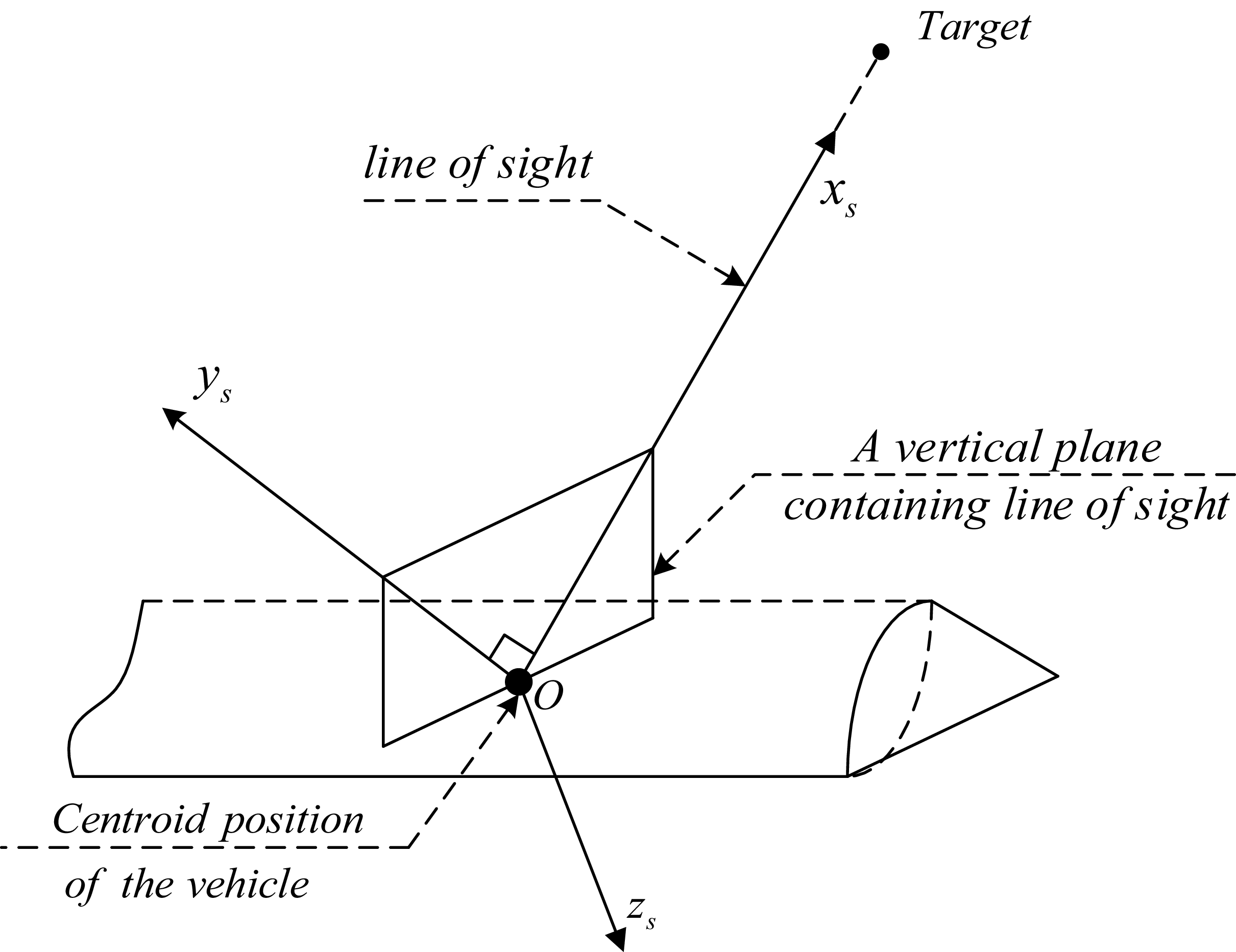
Inertial line-of-sight (LOS) coordinate systems
 $O{x_s}{y_s}{z_s}$
: The origin is selected at the centroid position of the vehicle.
 $O{x_s}$
coincides with the direction of the line of sight, and the direction pointing to the target is positive;
 $O{y_s}$
lies in the vertical plane containing the
 $O{x_s}$
and is perpendicular to it, with the positive direction being upward;
 $O{z_s}$
is determined by the right-hand rule. The coordinate systems is shown in Fig. 2.
Inertial LOS coordinate systems.

Note: The three frames defined above are local inertial frames attached to the vehicle and remain non-rotating relative to inertial space (translating only), in contrast to the coordinate systems commonly used in aerospace, such as ECEF, NED and body-fixed frames.
In the interception problem, different information needs to be measured in different coordinate systems, and in order for each physical quantity to be converted between different coordinate systems, the mutual conversion relationship between the implicated inertial coordinate systems and the inertial line of sight coordinate systems is given below.
The conversion relationship between the inertial line of sight frame and the implicated inertial frame is described by two angles, line of sight elevation and line of sight azimuth, which are defined as follows:
Definition 4.
Line of sight elevation
 ${q_\varepsilon }$
: the angle between the target line of sight and the plane of the implicated inertial coordinate systems
 $Oxz$
, which is positive if the line of sight is above the
 $Oxz$
, and negative otherwise.
Definition 5.
Line of sight azimuth
 ${q_\beta }$
: the angle between the projection of the target line of sight on the plane of the implicated inertial coordinate systems
 $Oxz$
and the
 $Ox$
axis. Looking in the direction of the
 $Oy$
axis, if the
 $Ox$
axis is turned counterclockwise to the LOS projection, the LOS azimuth is positive, and vice versa.
According to definitions 4 and 5, the inertial line of sight coordinate systems is obtained after two rotations with the reference to the implicated inertial coordinate systems, as shown in Fig. 3. From the rotation relation, the transformation matrix from the inertial frame to the inertial line of sight frame can be obtained as
 \begin{equation} L\left({{q_\varepsilon},{q_\beta }} \right) = \left[ {\begin{array}{*{20}{c@{\quad}c@{\quad}c}}{\cos {q_\varepsilon }\cos {q_\beta }} & {}{\sin {q_\varepsilon }}& {}{ - \cos {q_\varepsilon }\sin {q_\beta }}\\{ - \sin {q_\varepsilon }\cos {q_\beta }} & {}{\cos {q_\varepsilon }}& {}{\sin {q_\varepsilon }\sin {q_\beta }}\\{\sin {q_\beta }}& {}0 {}& {\cos {q_\beta }}\end{array}} \right]\end{equation}
The rotational relationship between the inertial LOS coordinate systems and the associated inertial coordinate systems.

2.2 Description of area coverage problems
The following describes the interception problem as a region coverage problem based on target manoeuvering and motion information detection errors. The definition and mathematical description of interceptor interceptable region and target predicted manoeuvering escape region are given, and the interceptor interceptable region is used to cover the target predicted manoeuvering escape region.
In the course of interception, when the interceptor and the target are relatively far away, the LOS angular rate is approximately 0, so the change of LOS angle can be ignored, and the interceptor motion model is established based on the LOS coordinate systems at the initial moment.
In the LOS reference frame, note that the interceptor position vector is
 $\boldsymbol{x}_{m} = {({x_m},{y_m},{z_m})^{\rm{T}}}$
, the velocity vector is
 $\boldsymbol{V}_{m} = {[{V_{mx}},{V_{my}},{V_{mz}}]^{\rm{T}}}$
Let
 $\boldsymbol{X}_{m} = {\left[ \boldsymbol{x}_{m}^{T},\boldsymbol{V}_{m}^{T} \right]^T}$
, then the interceptor model of motion is
 \begin{equation} {\dot{\boldsymbol{X}}_{m}} = {A_m}{\boldsymbol{X}_m} + {B_m}{U_m}\end{equation}
Where,
 ${A_m},{B_m}$
is
 \begin{equation*}{A_m} = \left[ {\begin{array}{*{20}{c}}{{0_{3 \times 3}}} \quad {}{{I_{3 \times 3}}}\\{{0_{3 \times 3}}} \quad {{0_{3 \times 3}}}\end{array}} \right],{\rm{ }}{B_m} = \left[ {\begin{array}{*{20}{c}}{{0_{3 \times 3}}}\\{{I_{3 \times 3}}}\end{array}} \right]\end{equation*}
 ${0_{3 \times 3}},{I_{3 \times 3}}$
are respectively a 3 × 3 zero matrix and a 3 × 3 identity matrix.
Although the interceptor’s dynamic characteristics do affect the size and shape of the interceptable region, including these dynamics would make the region time-varying and prevent any closed-form solution. Therefore, this study models the interceptor as a point mass. Moreover, any error in estimating the region’s extent only affects the number of missiles required; as long as this estimation error remains small, it will not materially impact the required interceptor count or undermine the validity of the proposed area-coverage method.
 ${{\bf{U}}_m} = {\left({{a_{mx}},{a_{my}},{a_{mz}}} \right)^T}$
is the acceleration vector for the interceptor. The acceleration of the interceptor has some saturation constraints due to physical constraints, noting that the maximum acceleration in the
 $O{x_s},O{y_s},O{z_s}$
direction of the reference frame is
 ${a_{\max }}$
, then the interceptor input constraints are integrated as:
 \begin{equation}{{\bf{U}}_m} = \left\{ {{{\bf{U}}_m}\left| {|{a_{mx}}| \le {a_{\max }},|{a_{my}}| \le {a_{\max }},|{a_{mz}}| \le {a_{\max }}} \right.} \right\}\end{equation}
The following definitions are given:
Definition 6.
Predicted hit time: The time when the interceptor is at minimum distance from the target in an uncontrolled state is called the predicted hit time, recorded as
 ${t_e}$
.
Assuming the interceptor maintains a parallel approach to the target, the predicted time of hit can be approximated as:
 \begin{equation}{t_e} = t + \frac{{{R_r}\left( t \right)}}{{{V_r}\left( t \right)}}\end{equation}
Where,
 ${R_r}\left( t \right)$
is the relative distance between the interceptor and the target at time
 $t$
,
 ${V_r}\left( t \right)$
is the magnitude of the target relative velocity component in the line of sight direction at time
 $t$
.
Definition 7.
Interceptor zero control terminal position: In the uncontrolled state (
 ${{\bf{U}}_m} = 0$
), the Interceptor position at time
 ${t_e}$
is called the zero-control terminal position.
Definition 8.
Interceptor interceptable area: The set of positions that the Interceptor can reach at time
 $t$
under the state of motion at time
 $t$
and the control after time
 ${t_e}$
is called the Interceptor interceptable area, denoted as
 $M\!\left(t\right)$
.
2.1.1 Interceptor interceptable region calculations
Record the coordinates of the interceptor zero control terminal position as
 ${{\bf{p}}_m} = {\left[ {\begin{array}{*{20}{c}}{{p_x}}\quad {}{{p_y}}\quad {}{{p_z}}\end{array}} \right]^T}$
, assume the initial state of motion of the vehicle to be
 ${X_m}\left({{t_0}} \right)$
, then from the Eq.:
 \begin{equation}{{\bf{p}}_m} = C{\Phi _m}\left({{t_e},{t_0}} \right){X_m}\left({{t_0}} \right)\end{equation}
Where,
 $C = \left[ {\begin{array}{*{20}{c}}{{I_{3 \times 3}}} {}\quad {{0_{3 \times 3}}}\end{array}} \right]$
,
 ${\Phi _m}\left({{t_e},{t_0}} \right)$
is the state transfer matrix for the interceptor motion model, i.e.
 \begin{equation}{\Phi _m}({t_e},{t_0}) = \left[ {\begin{array}{*{20}{c@{\quad}c}}{{I_{3 \times 3}}}& {}{({t_e} - {t_0}){I_{3 \times 3}}}\\{{0_{3 \times 3}}}& {}{{I_{3 \times 3}}}\end{array}} \right]\end{equation}
With constraints on input
 ${{\bf{U}}_m}\left( t \right)$
, the interceptor interceptable region at time
 ${t_0}$
can be represented as
 \begin{equation}M({t_0}) = \left\{ {{x_m}({t_e})\left| {{x_m}({t_e}) = C\left({{\Phi _m}({t_e},{t_0}){X_m}\left({{t_0}} \right) + \int_{{t_0}}^{{t_e}} {{\Phi _m}} ({t_e},\tau ){B_m}{{\bf{U}}_m}(\tau )d\tau}\right),{{\bf{U}}_m}(\tau ) \in {{\bf{U}}_m}} \right.} \right\}\end{equation}
Remark 1. [Reference Wang, Liu, Yao and He7]
 $M({t_0})$
is closely related to the initial moment, and if
 ${t_0}$
takes the mid to terminal guidance handover point, then is the interceptable region at mid to terminal guidance handover.
Lemma 1.
The relationship between the norms
 ${\left\| \bullet \right\|_2}$
and
 ${\left\| \bullet \right\|_1}$
is used in the derivation of the above equation, i.e.
 \begin{equation}{\left\| \bullet \right\|_2} \le {\left\|\bullet \right\|_1} \le \sqrt n {\left\|\bullet \right\|_2}\end{equation}
Proof in Appendix: ‘Proof of Lemma 1’.
Lemma 2.
Let
 $f$
be an integrable real-valued function on the interval
 $\left[ {a,b} \right]$
Then
 \begin{equation}\left| {\int_a^b {f\left( x \right)dx} } \right| \le \int_a^b {\left| {f\left( x \right)} \right|dx} \end{equation}
Proof in Appendix: ‘Proof of Lemma 2’.
Substituting Eq. into the interceptable region defined by Equation ([Reference Wang, Liu, Yao and He7]) and taking the L2-norm of both sides yields:
 \begin{align}\begin{array}{l}{\left\| {{x_m}({t_e}) - {{\bf{p}}_m}} \right\|_2} = {\left\| {C\int_{{t_0}}^{{t_e}} {{\Phi _m}} ({t_e},\tau ){B_m}{{\vec U}_m}(\tau )d\tau } \right\|_2} = {\left\| {\int_{{t_0}}^{{t_e}} {({t_e} - \tau )} {I_{3 \times 3}}{{\vec U}_m}(\tau )d\tau } \right\|_2}\\[8pt] \qquad \qquad \qquad = {\left\| {\left[ {\begin{array}{*{20}{l}}{\int_{{t_0}}^{{t_e}} {({t_e} - \tau ){u_{mx}}(\tau )} d\tau }\\[8pt]{\int_{{t_0}}^{{t_e}} {({t_e} - \tau ){u_{my}}(\tau )} d\tau }\\[8pt]{\int_{{t_0}}^{{t_e}} {({t_e} - \tau ){u_{mz}}(\tau )} d\tau }\end{array}} \right]} \right\|_2} \end{array} \end{align}
From Lemma 1, it follows that:
 \begin{equation}\begin{array}{l}{\left\| {\left[ {\begin{array}{*{20}{c}}{\int_{{t_0}}^{{t_e}} {({t_e} - \tau ){u_{mx}}(\tau )} d\tau }\\[8pt]{\int_{{t_0}}^{{t_e}} {({t_e} - \tau ){u_{my}}(\tau )} d\tau }\\[8pt]{\int_{{t_0}}^{{t_e}} {({t_e} - \tau ){u_{mz}}(\tau )} d\tau }\end{array}} \right]} \right\|_2} \le {\left\| {\left[ {\begin{array}{*{20}{c}}{\int_{{t_0}}^{{t_e}} {({t_e} - \tau ){u_{mx}}(\tau )} d\tau }\\[8pt]{\int_{{t_0}}^{{t_e}} {({t_e} - \tau ){u_{my}}(\tau )} d\tau }\\[8pt]{\int_{{t_0}}^{{t_e}} {({t_e} - \tau ){u_{mz}}(\tau )} d\tau }\end{array}} \right]} \right\|_1}\\\\ = \left| {\int_{{t_0}}^{{t_e}} {({t_e} - \tau ){u_{mx}}(\tau )d\tau } } \right| + \left| {\int_{{t_0}}^{{t_e}} {({t_e} - \tau ){u_{my}}(\tau )d\tau } } \right| + \left| {\int_{{t_0}}^{{t_e}} {({t_e} - \tau ){u_{mz}}(\tau )d\tau } } \right|\end{array}\end{equation}
Because the control vector
 ${{\bf{U}}_m}\left( t \right)$
is constrained, assume
 \begin{equation}\begin{array}{c}{{\bf{U}}_m}\left( t \right) = {\left[ {\begin{array}{*{20}{c}}{{u_{mx}}\left( t \right)} {}{{u_{my}}\left( t \right)} {}{{u_{mz}}\left( t \right)}\end{array}} \right]^T}\\[12pt]{\left[ {\begin{array}{*{20}{c}}{\left| {{u_{mx}}\left( t \right)} \right|} {}{\left| {{u_{my}}\left( t \right)} \right|} {}{\left| {{u_{mz}}\left( t \right)} \right|}\end{array}} \right]^T} \le {\left[ {\begin{array}{*{20}{c}}{{a_{mx}}} {}{{a_{my}}} {}{{a_{mz}}}\end{array}} \right]^T}\end{array}\end{equation}
From Lemma 2 and Eq., it follows that:
 \begin{align} \begin{array}{l}\left| {\int_{{t_0}}^{{t_e}} {({t_e} - \tau ){u_{mx}}(\tau )d\tau } } \right| + \left| {\int_{{t_0}}^{{t_e}} {({t_e} - \tau ){u_{my}}(\tau )d\tau } } \right| + \left| {\int_{{t_0}}^{{t_e}} {({t_e} - \tau ){u_{mz}}(\tau )d\tau } } \right|\\[12pt] \le \int_{{t_0}}^{{t_e}} {({t_e} - \tau )|{u_{mx}}(\tau )} |d\tau + \int_{{t_0}}^{{t_e}} {({t_e} - \tau )|{u_{my}}(\tau )} |d\tau + \int_{{t_0}}^{{t_e}} {({t_e} - \tau )|{u_{m{\rm{z}}}}(\tau )} |d\tau \\[12pt] \le \int_{{t_0}}^{{t_e}} {({t_e} - \tau )} {a_{mx}}d\tau + \int_{{t_0}}^{{t_e}} {({t_e} - \tau )} {a_{my}}d\tau + \int_{{t_0}}^{{t_e}} {({t_e} - \tau )} {a_{m{\rm{z}}}}d\tau \\[12pt] = \frac{1}{2}{({t_e} - {t_0})^2}({a_{mx}} + {a_{my}} + {a_{mz}})\end{array} \end{align}
In Eq., only the maximum acceleration in each coordinate direction is used. Although actual interceptor dynamics involve coupling between axes, the maximum total acceleration and its direction can be decomposed into maximum axis-wise components. Therefore, this coupling does not compromise the validity of the analytical results.
For clarity, we define
 ${a_{\max }} = {a_{mx}} + {a_{my}} + {a_{mz}}$
solely for this paper, then
 \begin{equation}{\left\| {C\int_{{t_0}}^{{t_e}} {{\Phi _m}} ({t_e},\tau ){B_m}{{\bf{U}}_m}(\tau )d\tau } \right\|_2} \le \frac{1}{2}{a_{\max }}{\left({{t_e} - {t_0}} \right)^2}\end{equation}
Further, define
 $\hat R({t_e},{t_0}) = \frac{1}{2}{a_{\max }}{({t_e} - {t_0})^2}$
, therefore
 \begin{equation}{\left\| {{x_m}({t_e}) - {{\bf{p}}_m}} \right\|^2} = {\left\| {\int_{{t_0}}^{{t_e}} {C{\Phi _m}} ({t_e},\tau ){B_m}{{\bf{U}}_m}(\tau )d\tau } \right\|^2} \le \hat R{({t_e},{t_0})^2}\end{equation}
So, the interceptor interceptable area at time
 ${t_0}$
is
 \begin{equation}M({t_0}) = \left\{ {{x_m}({t_e})\left| {{{\left\| {{x_m}({t_e}) - {{\bf{p}}_m}} \right\|}^2} \le \hat R{{({t_e},{t_0})}^2}} \right.} \right\}\end{equation}
In the derivation, incorporating the interceptor’s velocity constrains would partially truncate the interceptable region defined by Eq. However, because this region is subsequently scaled, the final estimated region in Eq. still serves as a conservative superset of the true, speed-limited interceptable set. Therefore, omitting velocity constraints does not compromise the conservativeness of our approach. Since this paper focuses primarily on presenting the interception methodology, the velocity constraints of the interceptor in omitted intentionally.
Proposition 1. During interception, the interceptor interceptable region has the following properties:
-
1. If
${t_1} \lt {t_2}$
, then
$M\left({{t_2}} \right) \subset M\left({{t_1}} \right)$
. -
2. If the constraint set of the vehicle control inputs is a bounded closed set, then there is a time invariant control input
${{\bf{U}}_m}\left( \tau \right),\tau \in \left[ {t,{t_e}} \right]$
, such that the vehicle can reach any point within the intercept region
$M\!\left(t\right)$
.


Proof:
For property 1, if
 ${t_1} \lt {t_2}$
, then
 \begin{equation*}\hat R({t_e},{t_1}) = \frac{1}{2}{a_{\max }}{({t_e} - {t_1})^2} \ge \frac{1}{2}{a_{\max }}{({t_e} - {t_2})^2} = \hat R({t_e},{t_2})\end{equation*}
So
 $M\!\left({{t_2}} \right) \subset M\!\left({{t_1}} \right)$
.
For property 2, Under the assumption of constant control inputs, let
 $M'\!\left(t\right)$
denote the interceptor’s interceptable region. Since reaching any point on the boundary of the interceptable region
 $M\!\left(t\right)$
requires the interceptor to apply the control input at its maximum or minimum constant value,
 $M'\!\left(t\right)$
and
 $M\!\left(t\right)$
share the same boundary. Moreover, because the interceptor’s terminal position is a continuous function of the control input, and the admissible set of control inputs is a bounded closed set, both
 $M'\!\left(t \right)$
and
 $M\!\left(t\right)$
are bounded closed sets with no discontinuities in their interiors. Therefore,
 $M'\!\left(t \right) = M\!\left(t\right)$
. That is, for every point in the interior of
 $M\!\left(t\right)$
, there exists a constant control input that enables the interceptor to reach that point.
Remark 2.
 $\hat R({t_e},t)$
is the radius of the intercepted area, the radius of the intercepted ball, is an increasing function of
 ${t_{go}} = {t_e} - t$
, the smaller the
 ${t_{go}}$
, the smaller the interceptable region, and as it approaches the target, the interceptable region converges to a point.
2.1.2 Calculation of target predicted manoeuvering escape zone
Definition 9.
Target predicted manoeuvering escape zone: The collection of all possible position points of a target at the predicted hit time is called the target predicted manoeuvering escape zone, recorded as
 ${R_o}$
.
Given that the target information needs to be obtained by measurements from external sensors such as satellites, AWACS radars, or UAV radars, the target motion model will therefore resume in inertial coordinates, assuming the target model is:
 \begin{equation}{\dot X_T} = {A_T}{X_T} + {B_T}{{\bf{U}}_T}\end{equation}
where
 ${A_T},{B_T}$
and
 ${A_m},{B_m}$
are the systems matrix and the input matrix of the appropriate dimension, respectively.
The mean and variance of the control inputs are
 ${U_{{T_0}}}$
and
 $\sigma _{uT}^2$
, respectively, assuming that the target input and the motion state at the initial moment obey a Gauss distribution, the mean and covariance matrix of the initial moment motion state are
 ${X_T}\!\left({{t_0}} \right)$
and
 ${Q_{X_T}}\!\left({t_0} \right)$
, respectively.
Then the mean and covariance matrix of the target motion state at time
 ${t_e}$
are
 \begin{align}{X_T}({t_e}) = {\Phi _T}({t_e},{t_0}){X_{\rm{T}}}({t_0}) + \int_{{t_0}}^{{t_e}} {{\Phi _T}} ({t_e},\tau ){B_T}{{\bf{U}}_{{T_0}}}d\tau . \nonumber\\[-25pt] \end{align}
 \begin{align}\begin{array}{l}{Q_{{X_T}}}({t_e}) = {\Phi _T}({t_e},{t_0}){Q_{{X_T}}}({t_0}){\Phi _T}{({t_e},{t_0})^{\rm{T}}} \\[8pt]\qquad \qquad+ \int_{{t_0}}^{{t_e}} {{\Phi _T}} ({t_e},\tau ){B_T}d\tau \cdot \sigma _{{U_T}}^2{\left({\int_{{t_0}}^{{t_e}} {{\Phi _T}} ({t_e},\tau ){B_T}d\tau } \right)^T}.\end{array} \\[6pt]\nonumber \end{align}
Therefore, the predicted target manoeuvering escape zone is
 \begin{equation}R = \left\{ {X\left| {X \sim N\left({{X_T}({t_e}),{Q_{{X_T}}}({t_e})} \right)} \right.} \right\}.\end{equation}
That is, the predicted target manoeuvering escape zone is an infinite region where state
 $X$
obeys mean
 ${X_T}({t_e})$
and variance
 ${Q_{{X_T}}}({t_e})$
. But in practical engineering applications, usually take a certain probability fall on a certain specific bounded region as the predicted target manoeuvering escape region, the following specific analysis and calculation of the approximate bounded region.
Proposition 2. The necessary and sufficient condition for an interceptor to be able to ensure a hit to a target in the presence of manoeuvering and motion information errors on the target is
 \begin{equation}\bar R(t) \le M(t),\quad \forall t \in [{t_0},{t_e}].\end{equation}
Since
 $M(t)$
is bounded, Eq. must approach this region
 $\bar R(t)$
with some particular bounded region, and
 $\bar R(t)$
must be the region projected onto the coordinate systems of line of sight.
Proof:
Sufficiency: By Proposition 1, at the terminal time
 ${t_f}$
, the region
 $M\!\left(t\right)$
collapses to a single point. Likewise, the target predicted manoeuvering escape zone
 $\bar R(t)$
also reduces to a single point. Since both sets are isolated singletons, if Eq. is satisfied at
 ${t_f}$
, the target’s position coincides with that of the interceptor, which implies a successful interception.
Necessity: If at some time
 $\tilde t \lt {t_e}$
there exists a point in
 $\bar R(t)$
that lies outsides the interceptor interceptable region
 $M\!\left(t\right)$
, then the target may follow a trajectory whose terminal position falls outside
 $M\!\left(t\right)$
. Under such a trajectory, the interceptor would fail to intercept the target. Therefore, to guarantee interception, the interceptor interceptable region must fully cover the target predicted manoeuvering escape zone at every instant prior to the encounter.
2.1.3 An approximate calculation for target predicted manoeuvering escape zone
Definition 10. Target-interceptor encounter plane: In three dimensions, the plane passing through the interceptor zero control terminal location and perpendicular to the line of sight is called the target interceptor encounter plane, simply the encounter plane or target plane.
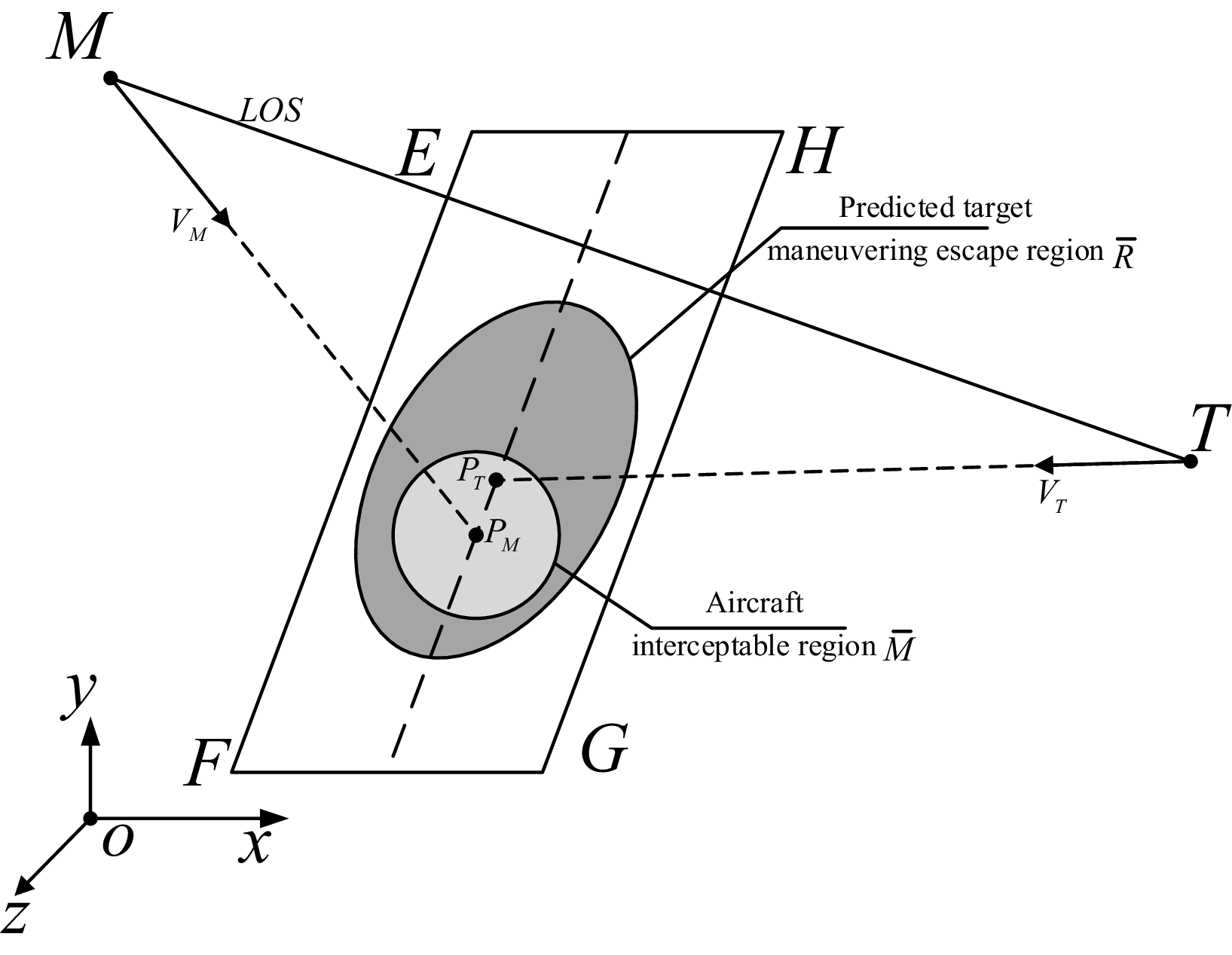
Since the component of target manoeuver and motion information error in the direction of line of sight only has some effect on the predicted hit time, it will not cause guidance bias; whereas a component in the direction perpendicular to the line of sight would cause a guidance bias, the interceptor acceleration would typically be perpendicular to the line of sight. The component of the target manoeuver and motion information error in the line of sight direction is negligible compared to the target-interceptor relative distance, so the effect of the target manoeuver and motion error on the predicted hit time can be ignored, and both the predicted target manoeuver escape region and the interceptor interceptable region are projected into the encounter plane, thus converting the coverage of the predicted manoeuver escape region in 3D space into the in-plane area coverage. In three dimensions, the interceptor interception geometry is shown in Fig. 4, where
 $M$
and
 $T$
represent the interceptor and target, respectively.
 ${p_m}$
is the interceptor zero control terminal location, and plane
 $EFGH$
is the encounter plane,
 ${p_T}$
is the projection of the mean point of the predicted manoeuver escape on the plane
 $EFGH$
,
 $\bar R$
and
 $\bar M$
are the projections of the manoeuvering escape region and the interceptor interceptable region in plane
 $EFGH$
, respectively,
 ${{\bf{V}}_m}$
and
 ${{\bf{V}}_T}$
are velocity vectors for the interceptor and target, respectively.
Interceptor interception geometry.

Since the vehicle motion model is established in the LOS reference frame, the projection of the interceptor interceptable region in plane
 $EFGH$
can be expressed as
 \begin{equation}\bar M\!\left(t\right) = \left\{ {\left({y,z} \right)\left| {{{\left| {y - {p_y}} \right|}^2} + {{\left| {z - {p_z}} \right|}^2} \le R{{\left({{t_e},{t_0}} \right)}^2}} \right.} \right\}.\end{equation}
That is, a disk with
 $\left({{p_y},{p_z}} \right)$
as the centre and
 $\hat R\left({{t_e},{t_0}} \right)$
as the radius.
For a predicted target manoeuvering escape region in the inertial coordinate systems, the projection in plane
 $EFGH$
is obtained by coordinate transformation as:
 \begin{equation}\bar R = \left\{ {\left({y,z} \right)\left| {\left({y,z} \right) \sim N\left({{\bf{y}},{Q_y}} \right)} \right.} \right\}\end{equation}
where,
 \begin{equation}{\bf{y}} = \left[ {\begin{array}{*{20}{c@{\quad}c@{\quad}c}} 0&1 & {}0\\[10pt]0 &0 & 1\end{array}} \right]L\left({{q_\varepsilon},{q_\beta }} \right)\left({\left[ {\begin{array}{*{20}{c}}{{x_T}\left({{t_e}} \right)}\\{{y_T}\left({{t_e}} \right)}\\{{z_T}\left({{t_e}} \right)}\end{array}} \right] - \left[ {\begin{array}{*{20}{c}}{{x_{{s_0}}}}\\[5pt]{{y_{{s_0}}}}\\[5pt]{{z_{{s_0}}}}\end{array}} \right]} \right)\end{equation}
 \begin{equation}{Q_y} = \left({\left[ {\begin{array}{*{20}{c@{\quad}c@{\quad}c}}0 {}& 1 & {}0\\[5pt]0 {}& 0 {}& 1 \end{array}} \right]L\left({{q_\varepsilon},{q_\beta }} \right)} \right){Q_{{x_T}}}\left({{t_e}} \right){\left({\left[ {\begin{array}{*{20}{c@{\quad}c@{\quad}c}}0 {}& 1& 0\\[5pt]0 & {}0 {}& 1\end{array}} \right]L\left({{q_\varepsilon},{q_\beta }} \right)} \right)^T}\end{equation}
where,
 $L\left({{q_\varepsilon},{q_\beta }} \right)$
is the transformation matrix from the inertial coordinate systems to the line of sight coordinate systems,
 ${\left[ {{x_{{s_0}}},{y_{{s_0}}},{z_{{s_0}}}} \right]^T}$
is the coordinate of the origin of the datum line of sight coordinate systems in the inertial coordinate systems,
 ${\left[ {{x_T}\!\left({{t_e}}\right)\!,{y_T}\left({{t_e}}\right)\!,{z_T}\!\left({{t_e}}\right)}\right]^T}$
is the coordinate of the mean point of the manoeuvering escape region in the inertial coordinate systems, and
 ${Q_{{x_T}}}\!\left({{t_e}}\right)$
is the covariance matrix of the manoeuvering escape region in the inertial coordinate systems.
The projection region
 $\bar R$
is analysed below.
The coefficient matrix
 ${A_T},{B_T}$
of the objective Eq. is the same as
 ${A_m},{B_m}$
. Therefore, the expression of the target state equation is similar to the vehicle state equation expression. i.e.
 ${{\bf{X}}_T}({t_e}) = \left({\begin{array}{*{20}{c}}{{{\bf{x}}_T}\left({{t_e}} \right)}\\{{{\bf{V}}_T}\left({{t_e}} \right)}\end{array}} \right)$
, of which
 ${{\bf{x}}_T}\left({{t_e}} \right) = \left({\begin{array}{*{20}{c}}{{x_T}\left({{t_e}} \right)}\\{{y_T}\left({{t_e}} \right)}\\{{z_T}\left({{t_e}} \right)}\end{array}} \right),{{\bf{V}}_T}\left({{t_e}} \right) = \left({\begin{array}{*{20}{c}}{{V_{{x_T}}}\left({{t_e}} \right)}\\{{V_{{y_T}}}\left({{t_e}} \right)}\\{{V_{{z_T}}}\left({{t_e}} \right)}\end{array}} \right)$
so
 \begin{equation}{{\bf{x}}_T}\left({{t_e}} \right) = \left[ {\begin{array}{*{20}{c}}{{I_{3 \times 3}}} \quad {}{{{\rm{O}}_{3 \times 3}}}\end{array}} \right]{{\bf{X}}_T}({t_e}) \buildrel \Delta \over = C{{\bf{X}}_T}({t_e})\end{equation}
where
 $C = \left[ {\begin{array}{*{20}{c}}{{I_{3 \times 3}}} {}{{{\rm{0}}_{3 \times 3}}}\end{array}} \right]$
.
Thus, the mean and covariance of the target location is:
 \begin{align}{{\bf{x}}_T}\left({{t_e}} \right) = C{\Phi _T}({t_e},{t_0}){{\bf{X}}_T}({t_0}) + C\int_{{t_0}}^{{t_e}} {{\Phi _T}} ({t_e},\tau ){B_T}{{\bf{U}}_{{T_0}}}d\tau \\[-40pt] \nonumber \end{align}
 \begin{align}{Q_{{x_T}}}\left({{t_e}} \right) & = C{\Phi _T}({t_e},{t_0}){Q_{{x_T}}}({t_0}){\left({{\Phi _T}({t_e},{t_0})C} \right)^T} \nonumber\\[6pt]&\quad+ \int_{{t_0}}^{{t_e}} C {\Phi _T}({t_e},\tau ){B_T}d\tau \cdot \sigma _{{u_T}}^2{\left({\int_{{t_0}}^{{t_e}} C {\Phi _T}({t_e},\tau ){B_T}d\tau } \right)^T} \end{align}
The initial errors of the target position typically originate from separate measurement channels with independent noise sources and can therefore be assumed independent of each other; likewise, the control vector undergoes an orthogonal decomposition in the inertial coordinate systems, allowing its components to be considered independent, i.e.
 \begin{equation*}\begin{array}{l}{Q_{{x_T}}}({t_0}) = \left[ {\begin{array}{*{20}{c@{\quad}c}}{\sigma _{\vec x}^2{{\left({{t_0}} \right)}_{3 \times 3}}} {}& {{0_{3 \times 3}}}\\[8pt]{{0_{3 \times 3}}} & {}{\sigma _{\vec V}^2{{\left({{t_0}} \right)}_{3 \times 3}}}\end{array}} \right],\sigma _{\vec x}^2\left({{t_0}} \right) = \left[ {\begin{array}{*{20}{c@{\quad}c@{\quad}c}}{\sigma _x^2\left({{t_0}} \right)} {} && {}\\& {}{\sigma _y^2\left({{t_0}} \right)}& {}\\&& {} {}{\sigma _z^2\left({{t_0}} \right)}\end{array}} \right]\\[16pt]\sigma _{\vec V}^2\left({{t_0}} \right) = \left[ {\begin{array}{*{20}{c@{\quad}c@{\quad}c}}{\sigma _{{V_x}}^2\left({{t_0}} \right)} {}&& {}\\& {}{\sigma _{{V_y}}^2\left({{t_0}} \right)}& {}\\&& {} {}{\sigma _{{V_z}}^2\left({{t_0}} \right)}\end{array}} \right],\sigma _{{u_T}}^2 = \left[ {\begin{array}{*{20}{c@{\quad}c@{\quad}c}}{\sigma _{{u_x}}^2} {}&& {}\\& {}{\sigma _{{u_y}}^2} {}&\\&& {} {}{\sigma _{{u_z}}^2}\end{array}} \right]\end{array}\end{equation*}
Due to
 ${\Phi _T}({t_e},{t_0}) = \left[ {\begin{array}{*{20}{c@{\quad}c}}{{I_{3 \times 3}}} {}& {\left({{t_e} - {t_0}} \right){I_{3 \times 3}}}\\{{0_{3 \times 3}}} {}& {{I_{3 \times 3}}}\end{array}} \right],C = \left[ {\begin{array}{*{20}{c}}{{I_{3 \times 3}}}\qquad {}{{{\rm{0}}_{3 \times 3}}}\end{array}} \right],{B_T} = \left[ {\begin{array}{*{20}{c}}{{{\rm{0}}_{3 \times 3}}}\\{{I_{3 \times 3}}}\end{array}} \right] $
, so
 \begin{align}{{\bf{x}}_T}\!\left({{t_e}} \right) = {{\bf{x}}_T}\!\left({{t_0}} \right) + ({t_e} - {t_0}){{\bf{V}}_T}\!\left({{t_0}} \right) + \frac{1}{2}{({t_e} - {t_0})^2}{{\bf{U}}_T}\!\left({{t_0}} \right) \\[-30pt] \nonumber \end{align}
 \begin{equation}\begin{array}{l}C{\Phi _T}({t_e}, {t_0}){Q_{{x_T}}}({t_0}){\left({{\Phi _T}({t_e},{t_0})C} \right)^T}\\[10pt] = \left[ {\begin{array}{*{20}{c}}{{I_{3 \times 3}}} \quad {}{{0_{3 \times 3}}}\end{array}} \right]\left[ {\begin{array}{*{20}{c}}{{I_{3 \times 3}}} {}\quad {({t_e} - {t_0}){I_{3 \times 3}}}\\[8pt]{{0_{3 \times 3}}} \quad {}{{I_{3 \times 3}}}\end{array}} \right]\left[ {\begin{array}{*{20}{c}}{\sigma _{\vec x}^2\!{{\left({{t_0}}\right)}_{3 \times 3}}} \quad {}{{0_{3 \times 3}}}\\[10pt]{{0_{3 \times 3}}} \quad {}{\sigma _{\vec V}^2{{\left({{t_0}} \right)}_{3 \times 3}}}\end{array}} \right]\left[ {\begin{array}{*{20}{c}}{{I_{3 \times 3}}} \quad {}{{0_{3 \times 3}}}\\[10pt]{({t_e} - {t_0}){I_{3 \times 3}}} \quad {}{{I_{3 \times 3}}}\end{array}} \right]\left[ {\begin{array}{*{20}{c}}{{I_{3 \times 3}}} \\[5pt]{{0_{3 \times 3}}}\end{array}} \right]\\[18pt] = \left[ {\begin{array}{*{20}{c@{\quad}c@{\quad}c}}{\sigma _x^2\!\left({{t_0}} \right) + {{\left({{t_e} - {t_0}} \right)}^2}\sigma _{{V_x}}^2\!\left({{t_0}} \right)}& {}0& {}0\\[10pt] 0& {}{\sigma _y^2\left({{t_0}} \right) + {{\left({{t_e} - {t_0}} \right)}^2}\sigma _{{V_y}}^2\!\left({{t_0}} \right)} & {}0\\[10pt]0& {}0& {}{\sigma _z^2\left({{t_0}} \right) + {{\left({{t_e} - {t_0}} \right)}^2}\sigma _{{V_z}}^2\!\left({{t_0}} \right)}\end{array}} \right]\end{array}\end{equation}
As well as
 \begin{equation}\int_{{t_0}}^{{t_e}} C {\Phi _T}({t_e},\tau ){B_T}d\tau \cdot \sigma _{{u_T}}^2{\left({\int_{{t_0}}^{{t_e}} C {\Phi _T}({t_e},\tau ){B_T}d\tau } \right)^T} = \frac{1}{4}{({t_e} - {t_0})^4}\sigma _{{u_T}}^2 = \frac{1}{4}{({t_e} - {t_0})^4}\left[ {\begin{array}{*{20}{c@{\quad}c@{\quad}c}}{\sigma _{{u_x}}^2} {}&& \\& {}{\sigma _{{u_y}}^2}&\\& & {}{\sigma _{{u_z}}^2}\end{array}} \right].\end{equation}
Therefore
From Eq.:
 \begin{equation}\begin{array}{l}{Q_{{x_T}}}\!\left({{t_e}} \right) = C{\Phi _T}({t_e},{t_0}){Q_{{x_T}}}({t_0}){\left({{\Phi _T}({t_e},{t_0})C} \right)^T}\\[10pt] \qquad\qquad + \int_{{t_0}}^{{t_e}} C {\Phi _T}({t_e},\tau ){B_T}d\tau \cdot \sigma _{{u_T}}^2{\left({\int_{{t_0}}^{{t_e}} C {\Phi _T}({t_e},\tau ){B_T}d\tau } \right)^T}\\[10pt]\qquad\quad = \left[ {\begin{array}{*{20}{ccc}} {\sigma _x^2\left({{t_0}} \right)}&&\\[10pt]& {}{\sigma _y^2\left({{t_0}} \right)} {}&\\[10pt] {} && {}{\sigma _z^2\left({{t_0}} \right)}\end{array}} \right] + {\left({{t_e} - {t_0}} \right)^2} \left[ {\begin{array}{*{20}{ccc}} {\sigma _{{V_x}}^2\left({{t_0}} \right)} && \\[10pt]& {}{\sigma _{{V_y}}^2\left({{t_0}} \right)}&\\[10pt]&& {\sigma _{{V_z}}^2\left({{t_0}} \right)}\end{array}} \right] + \frac{1}{4}{({t_e} - {t_0})^4}\left[ {\begin{array}{*{20}{ccc}}{\sigma _{{u_x}}^2} && \\[10pt]& {\sigma _{{u_y}}^2}&\\[10pt] {}&& {\sigma _{{u_z}}^2}\end{array}} \right]\end{array}\end{equation}
 \begin{align}\begin{array}{l}{Q_y} = \left({\left[ {\begin{array}{*{20}{ccc}}0 {}&\quad 1 {}&\quad 0\\0 {}&\quad 0 &\quad {}1 \end{array}} \right]L\left({{q_\varepsilon},{q_\beta }} \right)} \right){Q_{{x_T}}}\left({{t_e}} \right){\left({\left[ {\begin{array}{*{20}{ccc}}0 &\quad {}1&\quad {}0\\0 &\quad 0 & \quad {}1 \end{array}} \right]L\left({{q_\varepsilon},{q_\beta }} \right)} \right)^T} \\[15pt] \quad = \left[ {\begin{array}{*{20}{c@{\quad}c}}{\bar \sigma _x^2\left({{t_e}} \right){{\sin }^2}{q_\varepsilon }{{\cos }^2}{q_\beta } + \bar \sigma _y^2\left({{t_e}} \right){{\cos }^2}{q_\varepsilon } + \bar \sigma _z^2\left({{t_e}} \right){{\sin }^2}{q_\varepsilon }{{\sin }^2}{q_\beta }}& {} * \\[10pt] * & {}{\bar \sigma _x^2\left({{t_e}} \right){{\sin }^2}{q_\beta } + \bar \sigma _z^2\left({{t_e}} \right){{\cos }^2}{q_\beta }}\end{array}} \right]\end{array} \\[7pt] \nonumber \end{align}
where
 \begin{equation}\begin{array}{l} * = - \bar \sigma _x^2\left({{t_e}} \right)\sin {q_\varepsilon }\sin {q_\beta }\cos {q_\beta } + \bar \sigma _z^2\left({{t_e}} \right)\sin {q_\varepsilon }\sin {q_\beta }\cos {q_\beta }\\[7pt]\bar \sigma _x^2\left({{t_e}} \right) = \sigma _x^2\left({{t_0}} \right) + {\left({{t_e} - {t_0}} \right)^2}\sigma _{{V_x}}^2\left({{t_0}} \right) + \frac{1}{4}{({t_e} - {t_0})^4}\sigma _{{u_x}}^2\\[10pt]\bar \sigma _y^2\left({{t_e}} \right) = \sigma _y^2\left({{t_0}} \right) + {\left({{t_e} - {t_0}} \right)^2}\sigma _{{V_y}}^2\left({{t_0}} \right) + \frac{1}{4}{({t_e} - {t_0})^4}\sigma _{{u_y}}^2\\[10pt]\bar \sigma _z^2\left({{t_e}} \right) = \sigma _z^2\left({{t_0}} \right) + {\left({{t_e} - {t_0}} \right)^2}\sigma _{{V_z}}^2\left({{t_0}} \right) + \frac{1}{4}{({t_e} - {t_0})^4}\sigma _{{u_z}}^2\end{array}\end{equation}
Since
 $ * = \left({ - \bar \sigma _x^2\left({{t_e}} \right) + \bar \sigma _z^2\left({{t_e}} \right)} \right)\sin {q_\varepsilon }\sin {q_\beta }\cos {q_\beta }$
, when
 ${q_\varepsilon},{q_\beta }$
is smaller,
 $\sin {q_\varepsilon } \approx 0,\sin {q_\beta } \approx 0$
and
 $ - \bar \sigma _x^2\left({{t_e}} \right) + \bar \sigma _z^2\left({{t_e}} \right)$
is also smaller, there are
 \begin{equation} * \approx 0\end{equation}
Thus
 \begin{equation}{Q_y} \approx \left[ {\begin{array}{*{20}{c@{\quad}c}}{\tilde \sigma _y^2\left({{t_e}} \right)} & {}0\\[8pt]0 & {}{\tilde \sigma _z^2\left({{t_e}} \right)}\end{array}} \right]\end{equation}
where
 \begin{equation}\begin{array}{l}\tilde \sigma _y^2\left({{t_e}} \right) = \bar \sigma _x^2\left({{t_e}} \right){\sin ^2}{q_\varepsilon }{\cos ^2}{q_\beta } + \bar \sigma _y^2\left({{t_e}} \right){\cos ^2}{q_\varepsilon } + \bar \sigma _z^2\left({{t_e}} \right){\sin ^2}{q_\varepsilon }{\sin ^2}{q_\beta }\\[12pt]\tilde \sigma _z^2\left({{t_e}} \right) = \bar \sigma _x^2\left({{t_e}} \right){\sin ^2}{q_\beta } + \bar \sigma _z^2\left({{t_e}} \right){\cos ^2}{q_\beta }\end{array}\end{equation}
Denote
 \begin{equation}\begin{array}{l}{{\bar y}_T}\left({{t_e}} \right) = - {x_T}\left({{t_e}} \right)\sin {q_\varepsilon }\cos {q_\beta } + {y_T}\left({{t_e}} \right)\cos {q_\varepsilon } + {z_T}\left({{t_e}} \right)\sin {q_\varepsilon }\sin {q_\beta }\\[12pt]{{\bar z}_T}\left({{t_e}} \right) = {x_T}\left({{t_e}} \right)\sin {q_\beta } + {z_T}\left({{t_e}} \right)\cos {q_\beta }\end{array}\end{equation}
Therefore
 \begin{equation}{\bf{y}} = \left[ {\begin{array}{*{20}{c}}{{{\bar y}_T}\left({{t_e}} \right)}\\[8pt]{{{\bar z}_T}\left({{t_e}} \right)}\end{array}} \right]\end{equation}
So the manoeuvering escape zone projected to
 $EFGH$
by the target location is
 \begin{equation}\bar R = \left\{ {\left({y,z} \right)\left| {\left({y,z} \right) \sim N\left({\bar y,{Q_y}} \right)} \right.} \right\}\end{equation}
where
 ${\bf{y}} = \left[ {\begin{array}{*{20}{c}}{{{\bar y}_T}\left({{t_e}} \right)}\\[5pt]{{{\bar z}_T}\left({{t_e}} \right)}\end{array}} \right],{Q_y} \approx \left[ {\begin{array}{*{20}{c@{\quad}c}}{\tilde \sigma _y^2\left({{t_e}} \right)}& {}0 \\[5pt]0& {}{\tilde \sigma _z^2\left({{t_e}} \right)}\end{array}} \right]$
.
Since
 $\bar R$
is an unbounded region and cannot be used in engineering, it can be approximated with a bounded region, approximating
 $\tilde R$
with
 $\bar R$
 \begin{equation}\tilde R = \left\{ {\left({y,z} \right)\left| {\left({y,z} \right) \sim N\left({\bar y,{Q_y}} \right),{{\left({\frac{{y - {{\bar y}_T}\left({{t_e}} \right)}}{{3\tilde \sigma _y^2\left({{t_e}} \right)}}} \right)}^2} + {{\left({\frac{{z - {{\bar z}_T}\left({{t_e}} \right)}}{{3\tilde \sigma _z^2\left({{t_e}} \right)}}} \right)}^2} \le 1} \right.} \right\}\end{equation}
If the sample point
 $\xi $
falls within
 $\bar R$
, it falls within the
 $\tilde R$
region by a probability above
 $99\% $
. Further,
 $\tilde R$
can be divided into three regions
 ${\tilde R_1},{\tilde R_2},{\tilde R_3}$
.
 \begin{equation*}\begin{array}{l}{{\tilde R}_1} = \left\{ {\left({y,z} \right)\left| {\left({y,z} \right) \sim N\left({\bar y,{Q_y}} \right),{{\left({\frac{{y - {{\bar y}_T}\left({{t_e}} \right)}}{{\tilde \sigma _y^2\left({{t_e}} \right)}}} \right)}^2} + {{\left({\dfrac{{z - {{\bar z}_T}\left({{t_e}} \right)}}{{\tilde \sigma _z^2\left({{t_e}} \right)}}} \right)}^2} \le 1} \right.} \right\}\\[16pt]{{\tilde R}_2} = \left\{ {\left({y,z} \right)\left| {\left({y,z} \right) \sim N\left({\bar y,{Q_y}} \right),{{\left({\frac{{y - {{\bar y}_T}\left({{t_e}} \right)}}{{\tilde \sigma _y^2\left({{t_e}} \right)}}} \right)}^2} + {{\left({\dfrac{{z - {{\bar z}_T}\left({{t_e}} \right)}}{{\tilde \sigma _z^2\left({{t_e}} \right)}}} \right)}^2} \le 4} \right.} \right\}\backslash {{\tilde R}_1}\\[16pt]{{\tilde R}_3} = \left\{ {\left({y,z} \right)\left| {\left({y,z} \right) \sim N\left({\bar y,{Q_y}} \right),{{\left({\frac{{y - {{\bar y}_T}\left({{t_e}} \right)}}{{\tilde \sigma _y^2\left({{t_e}} \right)}}} \right)}^2} + {{\left({\dfrac{{z - {{\bar z}_T}\left({{t_e}} \right)}}{{\tilde \sigma _z^2\left({{t_e}} \right)}}} \right)}^2} \le 9} \right.} \right\}\backslash {{\tilde R}_2}\end{array}\end{equation*}
Thus
 \begin{equation}\tilde R = {\tilde R_1} \cup {\tilde R_2} \cup {\tilde R_3},{\rm{ }}{\tilde R_1} \cap {\tilde R_2} \cap {\tilde R_3} = \emptyset \end{equation}
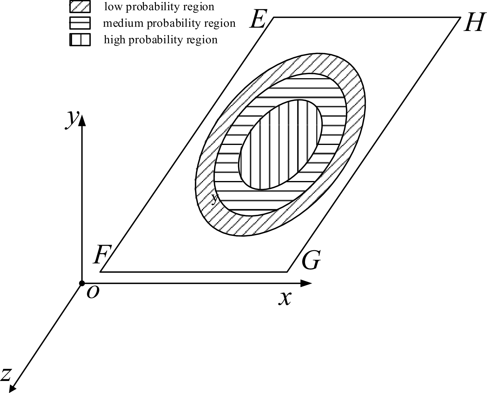
 ${\tilde R_1}$
is called the high probability region,
 ${\tilde R_2}$
is the medium probability region,
 ${\tilde R_3}$
is the low probability zone.
That means that the probability of
 ${\tilde R_1}$
target appearing within a region is highest, followed by at
 ${\tilde R_2}$
and lower at
 ${\tilde R_3}$
. Lowest in other areas, below
 $1\% $
, this area is no longer considered in engineering.
Therefore,
 $\tilde R$
is an ellipse on
 $EFGH$
, with the centre at
 $\left({{{\bar y}_T}\left({{t_e}} \right),{{\bar z}_T}\left({{t_e}} \right)} \right)$
, the long semi-axis at
 $3\tilde \sigma _y^2\left({{t_e}} \right)$
, and the short semi-axis at
 $3\tilde \sigma _z^2\left({{t_e}} \right)$
. Divide
 $\tilde R$
into three regions as shown in Fig. 5:
High, medium and low probability zone division map.

 ${\tilde R_1}$
is an ellipse with long semi-axis
 $\tilde \sigma _y^2\left({{t_e}} \right)$
and short semi-axis
 $\tilde \sigma _z^2\left({{t_e}} \right)$
;
 ${\tilde R_2}$
is an ellipse minus
 ${\tilde R_1}$
with long semi-axis
 $2\tilde \sigma _y^2\left({{t_e}} \right)$
and short semi-axis
 $2\tilde \sigma _z^2\left({{t_e}} \right)$
;
 ${\tilde R_3}$
is an ellipse minus
 ${\tilde R_2}$
with long semi-axis
 $3\tilde \sigma _y^2\left({{t_e}} \right)$
and short semi-axis
 $3\tilde \sigma _z^2\left({{t_e}} \right)$
.
2.1.4 Covering functions and interceptable probabilities
For a point
 $\xi = {\left[ {{\xi _y}, \, {\xi _z}} \right]^T} \in \bar R$
within the target manoeuvering escape region,
 $\phi \left( \xi \right)$
is defined as a function that represents the probability of the target eventually appearing at that point, and according to the covariance matrix of the projection of the target manoeuvering escape region, the expression for
 $\phi \left( \xi \right)$
can be
 \begin{equation}\phi \left( \xi \right) = \frac{1}{{2\pi {{\left({\det {Q_y}} \right)}^{\frac{1}{2}}}}}\exp \left\{ { - \frac{1}{2}{{\left({\xi - y} \right)}^T}Q_y^{ - 1}\left({\xi - y} \right)} \right\}\end{equation}
From Eq., then
 \begin{equation}\phi \left( \xi \right) = \frac{1}{{2\pi {{\tilde \sigma }_y}\left({{t_e}} \right){{\tilde \sigma }_z}\left({{t_e}} \right)}}\exp \left\{ { - \frac{1}{2}\left[ {{{\left({\frac{{{\xi _y} - {{\bar y}_T}\left({{t_e}} \right)}}{{{{\tilde \sigma }_y}\left({{t_e}} \right)}}} \right)}^2} + {{\left({\frac{{{\xi _z} - {{\bar z}_T}\left({{t_e}} \right)}}{{{{\tilde \sigma }_z}\left({{t_e}} \right)}}} \right)}^2}} \right]} \right\}\end{equation}
In the target-interceptor encounter plane, if point
 $\xi = {\left[ {{\xi _y},{\xi _z}} \right]^T} \in \bar R$
is within the interceptor interceptable region, then
 $\xi $
should satisfy:
 \begin{equation}{\left({{\xi _y} - {y_m}\left({{t_e}} \right)} \right)^2} + {\left({{\xi _z} - {z_m}\left({{t_e}} \right)} \right)^2} \le \hat R{\left({{t_e},{t_0}} \right)^2}.\end{equation}
Define
 $f\left({{\xi _y},{\xi _z},{y_m}\left({{t_e}}\right)\!,{z_m}\left({{t_e}} \right)} \right)$
to represent the interceptor coverage function, then
 \begin{equation}f\left({{\xi _y},{\xi _z},{y_m}\left({{t_e}} \right),{z_m}\left({{t_e}} \right)} \right) = \left\{ \begin{array}{c@{\quad}c}1 & {\rm{if}}{\left({{\xi _y} - {{\bar y}_m}\left({{t_e}} \right)} \right)^2} + {\left({{\xi _z} - {{\bar z}_m}\left({{t_e}} \right)} \right)^2} \le \hat R{\left({{t_e},{t_0}} \right)^2}\\[8pt]0& {\rm{otherwise}}\end{array} \right.\end{equation}
The covering function
 $f\left({{\xi _y},{\xi _z},{y_m}\left({{t_e}} \right),{z_m}\left({{t_e}} \right)} \right)$
describes the covering relationship between the interceptor position and point
 $\xi $
, and if
 $f\left({{\xi _y},{\xi _z},{y_m}\left({{t_e}} \right),{z_m}\left({{t_e}} \right)} \right) = 1$
, then indicates that point
 $\xi $
is within the interceptor interceptable region.
-
• Interceptable probability
The probability of a target appearing within the interceptor interceptable region at time
 ${t_0}$
can be expressed as:
 \begin{equation}{J_1} = \int\!\!\!\int_{\bar R} {f\left({{\xi _y},{\xi _z},{y_m}\left({{t_e}}\right)\!,{z_m}\left({{t_e}} \right)} \right)\phi \left({{\xi _y},{\xi _z}} \right)d{\xi _y}d{\xi _z}} \end{equation}
Where
 ${J_1}$
is called the interceptable probability. If the interceptor interceptable region completely covers the predicted target manoeuvering escape region, then
 ${J_1} = 1$
.
This paper addresses an area-coverage problem by deriving the interceptable region for each interceptor and defining successful interception as the complete coverage of the target’s escape region by multiple interceptors. Missile miss distance is not considered. In fact, including miss distance would enlarge each interceptor’s interceptable region, thereby increasing the probability of interception.
Special case: If
 ${t_0}$
is the mid to terminal guidance handover point, the intercept probability is the mid to terminal guidance angle handover success probability.
Under conditions where the interceptor manoeuverability is determined, the size of
 ${J_1}$
depends on the interceptor zero control terminal position and target line of sight angle, so the probability of a successful mid to late shift can be improved by designing the interceptor zero control terminal position and line of sight angle.
-
• Shift handover performance of midcourse and terminal guidance
The amount of zero control miss of the interceptor relative to the target is considered below. In the target encounter plane, for a point
 $\xi $
within the predicted target manoeuvering escape region, the zero control miss relative to the interceptor is:
 \begin{equation}z = \left\| {\xi - {p_m}} \right\|\end{equation}
where
 ${p_m} = \left({{y_m}\left({{t_e}} \right),{z_m}\left({{t_e}} \right)} \right)$
is the interceptor zero control terminal location.
From the probability density distribution function of
 $\xi $
, the mathematical expectation of the magnitude of the zero-control miss is obtained as:
 \begin{align} {J_2} & = \int\!\!\!\int_{\bar R} {\left\| {\xi - {p_m}} \right\|\phi \left( \xi \right)d\xi }\nonumber \\ & = \int\!\!\!\int_{\bar R} {\sqrt {{{\left({{\xi _y} - {{\bar y}_m}\left({{t_e}} \right)} \right)}^2} + {{\left({{\xi _z} - {{\bar z}_m}\left({{t_e}} \right)} \right)}^2}} \phi \left({{\xi _y},{\xi _z}} \right)d{\xi _y}d{\xi _z}} \end{align}
In the line of sight coordinate systems, the size of
 ${J_2}$
is only related to the interceptor zero control terminal position. Therefore, by designing the interceptor zero control terminal position, the amount of zero control miss at mid to late shift can be reduced, thus improving mid to late shift performance.
For the interceptor problem, the smaller the zero effect miss at mid to end shift (
 ${t_0}$
takes mid to end shift time), the higher the vehicle’s hit probability to the target during the terminal guidance phase. In addition, to ensure that the interceptor has the capability to intercept a target during the terminal guidance phase, the interceptor interceptable area should cover the target manoeuvering escape area during mid to terminal shift handover, and if the interceptable area of a single interceptor is small, multiple interceptor coordination is required to ensure a successful mid to terminal shift handover.
3.0 Fast Computation of Cooperative Interception Zones for Multiple Aircraft
3.1 Fast computation method for area coverage
Since the target’s manoeuvering escape area on the target-interceptor engagement platform can be approximated as an ellipse, while the interceptable area of the interceptor is a circle, the area coverage optimisation problem aims to cover the elliptical region with the minimum number of circles. Considering high-, medium- and low-probability subregions, priority should be given to covering high-probability regions first, followed by medium- and low-probability regions. To determine the centres of the covering circles and align with engineering practicality, geometric equations are employed for optimal coverage computation. The study will investigate several scenarios based on the following cases:
Assume the elliptical equation is
 \begin{equation}\frac{{{y^2}}}{{{a^2}}} + \frac{{{z^2}}}{{{b^2}}} = 1\ {\rm{or}}\ \frac{{{{\left({y - {y_0}} \right)}^2}}}{{{a^2}}} + \frac{{{{\left({z - {z_0}} \right)}^2}}}{{{b^2}}} = 1\end{equation}
The equation of the circle is
 \begin{align}{y^2} + {z^2} = {R^2}\ {\rm{or}}\ {\left({y - {y_0}} \right)^2} + {\left({z - {z_0}} \right)^2} = {R^2} \\[-20pt] \nonumber \end{align}
-
1. Case 1.
$b \le R \le a$
(long semi-axis)

First, the interval
 $a \in \left[ {R, + \infty } \right)$
is partitioned into several subintervals, as shown below
 \begin{equation}a \in \left[ {\left({N - 1} \right)\sqrt {\frac{{{a^2}\left({{R^2} - {b^2}} \right)}}{{{a^2} - {b^2}}}} + R,{\rm{ }}N\sqrt {\frac{{{a^2}\left({{R^2} - {b^2}} \right)}}{{{a^2} - {b^2}}}} + R} \right]{\rm{ }},N = 1,2, \ldots \end{equation}
Determine the intersection points between the ellipse and the circle
 \begin{equation}\left\{ \begin{array}{l}\frac{{{y^2}}}{{{a^2}}} + \frac{{{z^2}}}{{{b^2}}} = 1\\[10pt]{y^2} + {z^2} = {R^2}\end{array} \right.\end{equation}
Obtain
 $y = \pm \sqrt {\frac{{{a^2}\left({{R^2} - {b^2}} \right)}}{{{a^2} - {b^2}}}} $
,
 $z = \pm \sqrt {\frac{{{b^2}\left({{a^2} - {R^2}} \right)}}{{{a^2} - {b^2}}}} $
.
If
 $N = 1$
, one disk can be used to cover the whole area, with the equations of the disk defined as:
 \begin{equation}{y^2} + {z^2} = {R^2}\end{equation}
If
 $N = 2$
, then, two additional disks can be used to cover the remaining area, with the equations of the disks defined as:
 \begin{equation}{\left({y - {y_1}} \right)^2} + {z^2} = {R^2},{y_1} = \pm 2\sqrt {\frac{{{a^2}\!\left({{R^2} - {b^2}} \right)}}{{{a^2} - {b^2}}}} \end{equation}
By mathematical induction, the finally result is:
If
 $R \le a \le N\sqrt {{{{a^2}\left({{R^2} - {b^2}} \right)} \over {{a^2} - {b^2}}}} + R$
, a total of
 $2\left({N - 1} \right) + 1$
disks with a radius of
 $R$
are required to cover the elliptical region, and the coordinates of the centrres of these
 $2\left({N - 1} \right) + 1$
disks are:
 \begin{equation}\left({ \pm i\sqrt {\frac{{{b^2}\!\left({{a^2} - {R^2}} \right)}}{{{a^2} - {b^2}}}} ,0} \right){\rm{ }},i = 0,1, \ldots ,N\end{equation}
-
2. Case 2.
$b = R;R \lt a \lt NR\cos \frac{\pi }{6},N \ge 2$

if
 $N = 2$
, the four disks are defined:
 ${\left({y \pm R\cos \frac{\pi }{6}} \right)^2} + {\left({z \pm R\sin \frac{\pi }{6}} \right)^2} = {R^2}$
, and the centres of the four disks are located at:
 $\left({ \pm R\cos \frac{\pi }{6}, \pm R\sin \frac{\pi }{6}} \right)$
.
Analogous to Case 1, by mathematical induction, the final result is:
If
 $b = R$
;
 $R \lt a \lt NR\cos \frac{\pi }{6}$
,
 $4\left({N - 1} \right)$
disks are required to cover the region, with their centres located at:
 \begin{equation}\left({ \pm iR\cos \frac{\pi }{6}, \pm R\sin \frac{\pi }{6}} \right){\rm{ }},i = 1,2, \cdots ,N - 1\end{equation}
Remark 3.
When
 $a$
satisfies certain conditions, it is also possible to cover the region with two disks. However, this requires calculating the intersection points of the rightmost and leftmost ellipses from the previous coverage step, followed by comparing these points with the radius of the disk
 $R$
to determine whether a single disk can achieve full coverage. The computation of the disk’s centre is highly complex, so in practice, this method is not adopted.
-
3. Case 3.
$b \gt R;R \lt a \lt NR\cos \frac{\pi }{6},N \ge 2$

Since the detailed derivation follows the same steps as in Case 1 and Case 2, it will not be repeated here. The final conclusion is as follows:
when
 $R \lt b \lt MR;R \lt a \le 2NR\cos \frac{\pi }{6} + R$
, a total of
 $\left({M + 1} \right)\left({2N - 1} \right)$
disks are needed to cover the ellipse, with their centres located at:
 \begin{equation}\left({ \pm 2iR\cos \frac{\pi }{6}, \pm jR} \right){\rm{ }},i = 1,2, \cdots ,N,j = 0,1, \cdots ,M - 1\end{equation}
Remark 4.
Circle will also be translated by
 $\left({{{\bar y}_T}\left({{t_e}} \right),{{\bar z}_T}\left({{t_e}} \right)} \right)$
, that is:
 $\left({ \pm 2iR\cos \frac{\pi }{6} + {{\bar y}_T}\left({{t_e}} \right), \pm jR + {{\bar z}_T}\left({{t_e}} \right)} \right)$
,
 $i = 1,2, \cdots ,N$
,
 $j = 0,1, \cdots ,M - 1$
Remark 5. For the coverage of high, medium and low probability regions, the high probability region is first covered using the method for covering elliptical areas as described above. To cover the medium probability region, the same approach is applied, utilising discs to cover the area from the top, bottom, left and right. Finally, for the low probability region, the same method used for the medium probability region is applied to achieve coverage.
4.0 Simulation and Analysis
To verify the effectiveness of the proposed rapid calculation method for cooperative interception zones of high-manoeuvering targets, a comparative study is conducted between the proposed region coverage rapid calculation method (hereinafter referred to as the ‘geometric method’) and the method based on Voronoi partitioning and optimisation (hereinafter referred to as the ‘optimisation method’) in Ref. [Reference Wang, Liu, Yao and He7] under different conditions. The comparison is based on the coverage of high-probability regions. The following simulation analysis is carried out in the MATLAB R2022a environment on an Intel Core i9-13900HX 2.20GHz processor. The initial simulation conditions are as follows:
The initial state covariance of the target is
 \begin{align*}\begin{array}{c}{Q_{{x_T}}}({t_0}) = \left[ {\begin{array}{*{20}{c@{\quad}c@{\quad}c@{\quad}c@{\quad}c@{\quad}c}}{\sigma _x^2\left({{t_0}} \right)}&&&&&\\& {}{\sigma _y^2\left({{t_0}} \right)} {}&&&&\\&& {}{\sigma _z^2\left({{t_0}} \right)} {}&&&\\&&& {}{\sigma _{{V_x}}^2\left({{t_0}} \right)}&&\\&&&& {}{\sigma _{{V_y}}^2\left({{t_0}} \right)}& \\&&&&& {}{\sigma _{{V_z}}^2\left({{t_0}} \right)}\end{array}} \right] \\[35pt] \nonumber\kern-8pt = \left[ {\begin{array}{*{20}{c@{\quad}c@{\quad}c@{\quad}c@{\quad}c@{\quad}c}}{{{1000}^2}}&&&&&\\& {}{{{1000}^2}} {}&&&&\\&& {}{{{1000}^2}} {}&&&\\&&& {}{{{100}^2}}&&\\&&&& {}{{{100}^2}}&\\&&&& & {{{100}^2}}\end{array}} \right]\end{array} \end{align*}
and the initial input (acceleration) covariance of the target is
 \begin{equation*}\sigma _{{u_T}}^2 = \left[ {\begin{array}{*{20}{c@{\quad}c@{\quad}c}}{\sigma _{{u_x}}^2} {}&&\\& {}{\sigma _{{u_y}}^2} {}&\\&& {}{\sigma _{{u_z}}^2}\end{array}} \right] = \left[ {\begin{array}{*{20}{c@{\quad}c@{\quad}c}}{{{\left({\frac{{10}}{3}} \right)}^2}} {}&&\\& {}{{{\left({\frac{{20}}{3}} \right)}^2}}&\\& & {}{{{\left({\frac{{10}}{3}} \right)}^2}}\end{array}} \right]\end{equation*}
The simulation results for the predicted target manoeuver escape regions with low, medium and high probability areas are shown in Fig. 6.
High, medium and low probability zone division map.

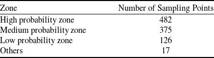
By sampling the predicted target manoeuver escape region using Eq., the number of sampling points is
 $n = 1000$
, and the sampling results are shown in Fig. 7.
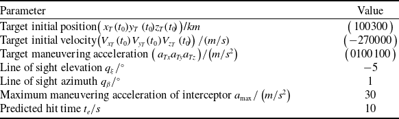
Initial simulation parameters

Table 1 Long description
The table presents initial simulation parameters and their corresponding values. It has two columns: Parameter and Value. The table includes the following rows: Row 1: Target initial position, (100 300 0) / km. Row 2: Target initial velocity, (-270000 0 0) / (m/s). Row 3: Target maneuvering acceleration, (0 100 100) / (m/s^2). Row 4: Line of sight elevation, 5 / degrees. Row 5: Line of sight azimuth, 1 / degrees. Row 6: Maximum maneuvering acceleration of interceptor, 30 / (m/s^2). Row 7: Predicted hit time, 10 / s.
Distribution of sampling point

Table 2 Long description
A table titled 'Distribution of sampling point' with two columns: Zone and Number of Sampling Points. The table has four rows of data. Row 1: High probability zone, 482. Row 2: Medium probability zone, 375. Row 3: Low probability zone, 126. Row 4: Others, 17.
Simulation time comparison

Table 3 Long description
A table comparing the simulation times of two methods. The table has two rows and two columns. The first column lists the methods: Geometric method and Optimisation method. The second column shows the corresponding simulation times: 0.160 seconds for the Geometric method and 6.185 seconds for the Optimisation method.
The number of sampling points in each region can be obtained by means of multiple samples, as shown in Table 2:
Result of sampling in target prediction manoeuvering escape area.

The number of sampling points in each probability area shown in Table 2 indicates that the method of approximating the target manoeuver escape regions using high, medium and low probability areas is reasonable.
The simulation results for the coverage of the high probability area using the geometric method and optimisation method are as follows:
The simulation time of the two methods is shown in Table 3:
From Fig. 8, it can be observed that for the elliptical predicted target escape region, the geometric method proposed in this paper achieves full coverage of the region and analytically provides the centre positions of the interceptable areas for each interceptor. In contrast, the optimisation method used in reference exhibits its variability in the simulation results for the same scenario due to the randomness of sampling and the subjectivity of the initial optimisation conditions, and it cannot guarantee full coverage of the region, as shown in Fig. 9. Additionally, as demonstrated in Table 3, the geometric method proposed in this paper significantly reduces the simulation time compared to the optimisation method, making it more suitable for real-time requirements in practical combat scenarios.
Result of high probability area coverage. (a) Geometric method. (b) Optimisation method.

Different results of optimisation method in the same case.

5.0 Conclusion
This paper presents a rapid geometric coverage-based approach for cooperative interception zones of interceptors against manoeuvering targets. By approximating the target’s manoeuvering escape area as an elliptical region and partitioning it into high-, medium- and low-probability subregions, the proposed method selectively covers these subregions using disk covering theory. The method analytically determines the number of interceptors required and the centre coordinates of each coverage disk.
Simulation results validate the correctness and effectiveness of the proposed approach. The findings demonstrate that for highly manoeuverable targets, the method achieves stable full coverage of the predicted escape region. Compared to conventional optimisation-based coverage methods, the algorithm significantly reduces computational time, thereby fulfilling the real-time requirements of practical combat operations.
Acknowledgements
The authors would like to thank the associate editor and reviewers for their valuable comments and constructive suggestions that helped to improve the paper and presentation significantly.
Appendix
Proof of Lemma 1: For any vector
 $x = \left({{x_1},{x_2},...,{x_n}} \right) \in {{\mathbb R}^n}$
, we have:
 \begin{equation*}\begin{array}{l}{\left\| x \right\|_1} = \sum\limits_{i = 1}^n {\left| {{x_i}} \right|} \\{\left\| x \right\|_2} = \sqrt {\sum\limits_{i = 1}^n {x_i^2} } \end{array}\end{equation*}
Since each
 $\left| {{x_i}} \right| \ge 0$
, we have
 \begin{equation*}{\left\| x \right\|_1} = \sum\limits_{i = 1}^n {\left| {{x_i}} \right|} \Rightarrow {\left({{{\left\| x \right\|}_1}} \right)^2} = {\left({\sum\limits_{i = 1}^n {\left| {{x_i}} \right|} } \right)^2} = \sum\limits_{i = 1}^n {{{\left| {{x_i}} \right|}^2}} + 2\sum\limits_{1 \le i \le j \le n} {\left| {{x_i}} \right|\left| {{x_j}} \right|} \ge \sum\limits_{i = 1}^n {{{\left| {{x_i}} \right|}^2}} = {\left({{{\left\| x \right\|}_2}} \right)^2}\end{equation*}
Taking square roots on both sides gives
 \begin{equation*}{\left\| x \right\|_2} \le {\left\| x \right\|_1}\end{equation*}
Apply the Cauchy–Schwarz inequality to the two n-dimensional vectors
 \begin{equation*}\left({\left| {{x_1}} \right|,\left| {{x_2}} \right|, \ldots ,\left| {{x_n}} \right|} \right)and\left({1,1,..,1} \right)\end{equation*}
By Cauchy–Schwarz,
 \begin{equation*}\sum\limits_{i = 1}^n {\left| {{x_i}} \right|} \cdot 1 \le \sqrt {\sum\limits_{i = 1}^n {{{\left| {{x_i}} \right|}^2}} } \cdot \sqrt {\sum\limits_{i = 1}^n {{1^2}} } \end{equation*}
But
 $\sum\limits_{i = 1}^n {\left| {{x_i}} \right|} \cdot 1 = {\left\| x \right\|_1},\sqrt {\sum\limits_{i = 1}^n {{{\left| {{x_i}} \right|}^2}} } = {\left\| x \right\|_2},\sqrt {\sum\limits_{i = 1}^n {{1^2}} } = \sqrt n $
, hence
 \begin{equation*}{\left\| x \right\|_1} \le \sqrt n {\left\| x \right\|_2}\end{equation*}
Combining the two results yields
 \begin{equation*}{\left\| x \right\|_2} \le {\left\| x \right\|_1} \le \sqrt n {\left\| x \right\|_2}\end{equation*}
as claimed.
Proof of Lemma 2: First, consider the properties of the function
 $f$
:
 \begin{equation*} - \left|\, {f\left(x\right)} \right| \le f\,\left(x \right) \le \left|\,{f\!\left(x \right)} \right|\end{equation*}
Then, consider the order-preserving property of integration, it follows that:
 \begin{equation*} - \int_a^b {\left|\, {f\!\left(x\right)} \right|dx} \le \int_a^b {f\!\left(x\right)dx} \le \int_a^b {\left|{\,f\!\left(x\right)} \right|dx} \end{equation*}
The above formula is equivalent to
 \begin{equation*}\left| {\int_a^b {f\!\left(x\right)dx} } \right| \le \int_a^b {\left|\, {f\!\left( x \right)} \right|dx} \end{equation*}
Therefore, Lemma 2 is proved.