1. Introduction
Taylor–Couette (TC) flow, i.e. the flow between two independently rotating concentric cylinders, has long been used as a model system in fluid dynamics. Couette (Reference Couette1890) was the first to investigate it, and he pioneered its usage as a viscometer. But it was Mallock (Reference Mallock1896) who, by rotating the inner cylinder, and not the outer as Couette had done, found the first indications of turbulence in the system. Taylor (Reference Taylor1923, Reference Taylor1936) further studied the system, finding that it was linearly unstable, unlike pipe-flow and other systems studied previously. Wendt (Reference Wendt1933) expanded the study of the turbulent regime, measuring torques and velocities in the system. Since then, and due to its simplicity, TC flow has been used as a model system for studying shear flows. For a broader historical context, we refer the reader to Donnelly (Reference Donnelly1991).
Recently, a mathematically exact analogy between TC flow and Rayleigh–Bénard flow (RB), i.e. the convective flow between two parallel plates heated from below and cooled from above was found by Eckhardt, Grossmann & Lohse (Reference Eckhardt, Grossmann and Lohse2007) (here referred to as EGL07). Within this context, TC flow can be viewed as a convective flow, driven by the shear between both cylinders where angular velocity is transported from the inner to the outer cylinder. As explained by Grossmann, Lohse & Sun (Reference Grossmann, Lohse and Sun2014), as long as the driving of the system is small, the transport is limited by the laminar boundary layers. But if the driving becomes strong enough the boundary layers become turbulent and the system enters the so-called ‘ultimate’ regime. The study of the transition to this regime, expected to be also present in RB flow, has attracted recent interest, as most applications of TC flow and RB flow in geophysics and astrophysics are expected to be in this ultimate regime.
For RB flow, the transition to an ultimate regime was first qualitatively predicted by Kraichnan (Reference Kraichnan1962), and later quantitatively by Grossmann & Lohse (Reference Grossmann and Lohse2000, Reference Grossmann and Lohse2001, Reference Grossmann and Lohse2011) and then experimentally found by He et al. (Reference He, Funfschilling, Bodenschatz and Ahlers2012a ,Reference He, Funfschilling, Nobach, Bodenschatz and Ahlers b ), Ahlers et al. (Reference Ahlers, He, Funfschilling and Bodenschatz2012), Roche et al. (Reference Roche, Gauthier, Kaiser and Salort2010). It lies outside the present reach of direct numerical simulation (DNS). The analogous boundary layer transition to an ultimate regime in TC flow was first found in the experiments by Lathrop, Fineberg & Swinney (Reference Lathrop, Fineberg and Swinney1992a ,Reference Lathrop, Fineberg and Swinney b ) and analysed more precisely by Lewis & Swinney (Reference Lewis and Swinney1999), even though earlier work by Wendt (Reference Wendt1933) already showed some transition in the torque scaling around the same Reynolds number. The transition was not related to the transition to the ultimate regime until later (van Gils et al. Reference van Gils, Huisman, Bruggert, Sun and Lohse2011; Paoletti & Lathrop Reference Paoletti and Lathrop2011; Huisman et al. Reference Huisman, van Gils, Grossmann, Sun and Lohse2012; Grossmann et al. Reference Grossmann, Lohse and Sun2014). In DNS, it was observed for the first time by Ostilla-Mónico et al. (Reference Ostilla-Mónico, van der Poel, Verzicco, Grossmann and Lohse2014b ).
In TC flow this transition is easier to achieve as the mechanical driving is more efficient than the thermal one, and thus the frictional Reynolds numbers in the boundary layer are much larger. By using the analogy between both systems, better understanding of the transition in TC flow can thus also lead to new insight in RB flow, where it is more elusive.
Ostilla-Mónico et al. (Reference Ostilla-Mónico, van der Poel, Verzicco, Grossmann and Lohse2014b
) numerically studied the transitions in TC flow for pure inner cylinder rotation for a radius ratio of
 ${\it\eta}=r_{i}/r_{o}=0.714$
, where
 $r_{o}$
and
 $r_{i}$
are the outer and inner radii, respectively, and an aspect ratio
 ${\rm\Gamma}=L/(r_{o}-r_{i})=2{\rm\pi}/3$
, where
 $L$
is the axial period in the DNS. In that study, the flow transitions and boundary-layer dynamics were revealed in the range of Taylor numbers
 $\mathit{Ta}$
between
 $10^{4}$
and
 $10^{10}$
), where the Taylor number is defined as
 $$\begin{eqnarray}\mathit{Ta}={\textstyle \frac{1}{4}}{\it\sigma}d^{2}(r_{o}+r_{i})^{2}({\it\omega}_{i}-{\it\omega}_{o})^{2}{\it\nu}^{-2},\end{eqnarray}$$
with
 ${\it\omega}_{o}$
and
 ${\it\omega}_{i}$
the angular velocities of the outer and inner cylinder, respectively,
 $d=r_{o}-r_{i}$
the gap width, and
 ${\it\nu}$
the kinematic viscosity of the fluid.
 ${\it\sigma}=$
 $[(r_{o}+r_{i})/(2\sqrt{r_{i}r_{o}})]^{4}$
can be considered as a geometric quasi-Prandtl number (EGL07).
We now describe the series of events when increasing
 $\mathit{Ta}$
. For small enough
 $\mathit{Ta}$
, the flow is in the purely azimuthal, laminar, state. When the system is driven beyond a critical driving, one passes the onset of instability and the purely azimuthal, laminar, flow disappears and large-scale Taylor rolls form. Further increasing of the driving breaks up these rolls, causing the onset of time-dependence as the system transitions from the stationary Taylor vortex regime to the modulated Taylor vortex regime and finally the breakup of these into chaotic turbulent Taylor vortices. These changes of the flow are reflected in transitions of the local scaling laws for the torque versus driving, i.e. versus Taylor number
 $\mathit{Ta}$
. All of this has been studied extensively and summarized, for example, by Andereck, Dickman & Swinney (Reference Andereck, Dickman and Swinney1983), Lathrop et al. (Reference Lathrop, Fineberg and Swinney1992a
,Reference Lathrop, Fineberg and Swinney
b
) and Lewis & Swinney (Reference Lewis and Swinney1999). The mentioned breakup of the rolls leads to the existence of a transitional regime, where the large-scale coherent structures still can be identified when looking at the time-averaged quantities. Looking at the details of the flow, a mixture of turbulent and laminar boundary layers is present.
In this transitional regime, hairpin vortices, which, in the context of RB flow, can also be viewed as plumes, are ejected from both inner and outer cylinders, and these contribute to large-scale bulk structures. These structures in turn cause an axial pressure gradient, which couples back to the boundary layers, causing plumes to be ejected there. But this only happens from preferential spots in the boundary layers. Once the driving is strong enough, the large-scale structures slowly vanish, and the plumes no longer feel an axial pressure gradient. The boundary layers now become fully turbulent and the flow transitions to the ‘ultimate’ regime. As the flow enters the ultimate regime, and the boundary layer become turbulent, a logarithmic signature in the angular velocity boundary layers is expected, which indeed has been found experimentally (Huisman et al. Reference Huisman, Scharnowski, Cierpka, Kähler, Lohse and Sun2013) and numerically (Ostilla-Mónico et al. Reference Ostilla-Mónico, van der Poel, Verzicco, Grossmann and Lohse2014b ).
In the ultimate regime, an effective scaling relation between the Nusselt number
 $Nu_{{\it\omega}}$
, i.e. the non-dimensional torque
 $Nu_{{\it\omega}}=T/T_{pa}$
where
 $T$
is the torque, and
 $T_{pa}$
the torque in the purely azimuthal state, and the Taylor number
 $\mathit{Ta}$
is expected, with an effective scaling exponent which exceeds that for the laminar-type boundary layer case (Malkus Reference Malkus1954), for which
 ${\it\alpha}={\textstyle \frac{1}{3}}$
. That is, in the ultimate regime, we expect an effective scaling law
 $Nu_{{\it\omega}}\sim \mathit{Ta}^{{\it\alpha}}$
with
 ${\it\alpha}>{\textstyle \frac{1}{3}}$
. In fact, for that regime, the relation law
 $Nu_{{\it\omega}}\sim \mathit{Ta}^{1/2}$
with logarithmic corrections was suggested (Kraichnan Reference Kraichnan1962; Spiegel Reference Spiegel1971; Grossmann & Lohse Reference Grossmann and Lohse2011). The logarithmic corrections are quite large, and lead to an effective scaling law with
 ${\it\alpha}\approx 0.38$
for
 $\mathit{Ta}\sim 10^{11}$
(Grossmann & Lohse Reference Grossmann and Lohse2011; van Gils et al.
Reference van Gils, Huisman, Grossmann, Sun and Lohse2012). We note that this scaling law is analogue to the scaling of the friction factor with Reynolds number in fully turbulent pipes Prandtl (Reference Prandtl1933).
For the largest drivings, remnants of the larger rolls, which can be seen as a large-scale wind, are still observed at even the largest Reynolds numbers studied numerically (Ostilla-Mónico et al.
Reference Ostilla-Mónico, van der Poel, Verzicco, Grossmann and Lohse2014b
), and experimentally, even up to
 $\mathit{Re}\sim 10^{6}$
(Huisman et al.
Reference Huisman, van der Veen, Sun and Lohse2014). In Ostilla-Mónico et al. (Reference Ostilla-Mónico, van der Poel, Verzicco, Grossmann and Lohse2014b
), the remnants of the large-scale structures played a crucial role in the transition to the ultimate regime. However, large-scale structures are not present in the whole parameter space of TC flow. Andereck, Liu & Swinney (Reference Andereck, Liu and Swinney1986) showed how rich a variety of different states exists at low Reynolds number when the outer cylinder is also rotated. Brauckmann & Eckhardt (Reference Brauckmann and Eckhardt2013b
) reported that the strength of the large-scale wind was most pronounced at the position of optimal transport. However, if the outer cylinder is counter-rotated past the position of optimal transport, bursts arise from the outer cylinder. The flow is very different outside and inside the neutral surface, which separates Rayleigh-stable from Rayleigh-unstable regions of the gap, changing completely the dynamics of the system. The Taylor vortices no longer penetrate the whole gap, extending thus the unstable region effectively somewhat outside the neutral surface of laminar-type flow (Ostilla-Mónico et al.
Reference Ostilla-Mónico, Stevens, Grossmann, Verzicco and Lohse2013).
The geometry of the system can be expected to play an important role in determining the strength of the large-scale wind, and how the transition takes place. In the context of understanding the radius-ratio dependence of the transition to the ultimate regime, Merbold, Brauckmann & Egbers (Reference Merbold, Brauckmann and Egbers2013) reported a higher transitional Reynolds numbers for
 ${\it\eta}=0.5$
than what was seen for
 ${\it\eta}=0.714$
by Ostilla-Mónico et al. (Reference Ostilla-Mónico, van der Poel, Verzicco, Grossmann and Lohse2014b
) and for
 ${\it\eta}=0.909$
by Ravelet, Delfos & Westerweel (Reference Ravelet, Delfos and Westerweel2010). Also the aspect ratio plays a role. Although different vortical states were known to coexist at low Reynolds number (Benjamin Reference Benjamin1978), it was previously thought that if the driving was sufficiently large, only one branch of the torque versus Taylor number curve would survive (Lewis & Swinney Reference Lewis and Swinney1999). Brauckmann & Eckhardt (Reference Brauckmann and Eckhardt2013a
) found that the difference in the global response between different vortical states becomes smaller with increasing Reynolds number. Recently, Martinez-Arias et al. (Reference Martinez-Arias, Peixinho, Crumeyrolle and Mutabazi2014) reported on the existence of different vortical states associated to different global torques at a given Taylor number for
 ${\it\eta}=0.909$
, and that there is a crossing between those torque-versus-
 $\mathit{Ta}$
curves around the transition to the ultimate regime. Furthermore, Huisman et al. (Reference Huisman, van der Veen, Sun and Lohse2014) showed that different vortical states survive up to Reynolds number of
 $10^{6}$
, corresponding to Taylor numbers of order
 $10^{12}$
. Furthermore, by combining measurements of global torque and local velocity, Huisman et al. (Reference Huisman, van der Veen, Sun and Lohse2014) found that the optimal transport is connected to the existence of the large-scale coherent structures at high Taylor numbers.
Therefore, some questions arise which we want to address in the present paper: How does the transition in the boundary layers take place across the full parameter space of TC flow? Is the vanishing of the large-scale wind a necessary and/or a sufficient condition for the boundary-layer transition? Why does the transition occur later for
 ${\it\eta}=0.5$
than for larger values of
 ${\it\eta}$
? Finally, what is the effect of the vortical wavelength and why do different branches of the torque-versus-Taylor-number scaling curves cross near the transition to the ultimate regime?
2. Explored parameter space
2.1. Control parameters
To answer these questions, DNS of TC flow have been performed across all dimensions of the parameter space, not only adding outer cylinder rotation, but also varying both geometrical parameters
 ${\it\eta}$
and
 ${\rm\Gamma}$
. To do this, the rotating-frame formulation of Ostilla-Mónico et al. (Reference Ostilla-Mónico, Stevens, Grossmann, Verzicco and Lohse2013) was used. In that paper, TC flow was formulated in a frame rotating with the outer cylinder, such that it looks like a system in which only the inner cylinder is rotating, but with a Coriolis force term, which represents the original presence of the outer cylinder rotation. The shear driving of the system is non-dimensionally expressed as a Taylor number, introduced previously:
 $$\begin{eqnarray}\mathit{Ta}={\textstyle \frac{1}{4}}{\it\sigma}d^{2}(r_{o}+r_{i})^{2}({\it\omega}_{i}-{\it\omega}_{o})^{2}{\it\nu}^{-2},\end{eqnarray}$$
 $\mathit{Ta}$
is the analogue to the Rayleigh number in RB flow, as elaborated in (EGL07). The outer cylinder rotation reflects in a Coriolis force, characterized by a Rossby number
 $\mathit{Ro}=|{\it\omega}_{o}-{\it\omega}_{i}|r_{i}/(2{\it\omega}_{o}d)$
. The Rossby number or rather
 $\mathit{Ro}^{-1}$
is the parameter which appears in the equations of motion for the fluid:
 $$\begin{eqnarray}\frac{\partial \tilde{\boldsymbol{u}}}{\partial \tilde{t}}+\tilde{\boldsymbol{u}}\boldsymbol{\cdot }\tilde{\boldsymbol{{\rm\nabla}}}\tilde{\boldsymbol{u}}=-\tilde{\boldsymbol{{\rm\nabla}}}\tilde{p}+\displaystyle \frac{f({\it\eta})}{\mathit{Ta}^{1/2}}\tilde{{\rm\nabla}}^{2}\tilde{\boldsymbol{u}}-\mathit{Ro}^{-1}\boldsymbol{e}_{z}\times \tilde{\boldsymbol{u}},\end{eqnarray}$$
where
 $f({\it\eta})=\frac{1}{4}{\it\sigma}((1+{\it\eta})/{\it\eta})^{2}$
, a geometrical parameter. The Rossby number is related to the frequency ratio
 ${\it\mu}={\it\omega}_{o}/{\it\omega}_{i}$
via
 $$\begin{eqnarray}\mathit{Ro}^{-1}=\text{sgn}({\it\omega}_{o})\left|\frac{{\it\mu}}{{\it\mu}-1}\right|\frac{2(1-{\it\eta})}{{\it\eta}}.\end{eqnarray}$$
Thus fixed
 $\mathit{Ro}^{-1}$
means fixed
 ${\it\mu}$
and vice versa. Here
 $\mathit{Ro}^{-1}>0$
describes co-rotation or
 ${\it\omega}_{o}>0$
, while
 $\mathit{Ro}^{-1}<0$
means counter-rotation. The radius ratio
 ${\it\eta}$
is presented by the geometrical amplitude factor
 $2(1-{\it\eta})/{\it\eta}$
, being small for small gap (
 ${\it\eta}\rightarrow 1$
) and large for large gap (
 ${\it\eta}\rightarrow 0$
). A resting outer cylinder is described by
 $\mathit{Ro}^{-1}=0$
.
There are also other ways of choosing the control parameters. Classically, they have been expressed as two non-dimensional Reynolds numbers corresponding to the inner and outer cylinders:
 $\mathit{Re}_{i,o}=u_{i,o}^{{\it\theta}}\cdot d/{\it\nu}$
, where
 $u_{i,o}^{{\it\theta}}$
are the azimuthal velocities of the inner and outer cylinders. The classical flow control parameters
 $(\mathit{Re}_{i},\mathit{Re}_{o})$
can be transformed to the
 $(\mathit{Ta},\mathit{Ro}^{-1})$
parameter space by
 $$\begin{eqnarray}\mathit{Ta}=f({\it\eta})|\mathit{Re}_{i}-{\it\eta}\mathit{Re}_{o}|^{2},\end{eqnarray}$$
and
 $$\begin{eqnarray}\mathit{Ro}^{-1}=\displaystyle \frac{2(1-{\it\eta})\mathit{Re}_{o}}{|{\it\eta}\mathit{Re}_{o}-\mathit{Re}_{i}|}.\end{eqnarray}$$
Vice versa, we have
 $$\begin{eqnarray}\mathit{Re}_{i}=\left(\displaystyle \frac{\mathit{Ta}}{f({\it\eta})}\right)^{1/2}\left(1+\displaystyle \frac{{\it\eta}\mathit{Ro}^{-1}}{2(1-{\it\eta})}\right),\end{eqnarray}$$
and
 $$\begin{eqnarray}\mathit{Re}_{o}=\displaystyle \frac{\mathit{Ro}^{-1}\mathit{Ta}^{1/2}}{2f({\it\eta})^{1/2}(1-{\it\eta})}.\end{eqnarray}$$
The driving can also be expressed as a shear Reynolds number
 $\mathit{Re}_{s}=\sqrt{\mathit{Ta }/{\it\sigma}}$
.
2.2. Numerical scheme
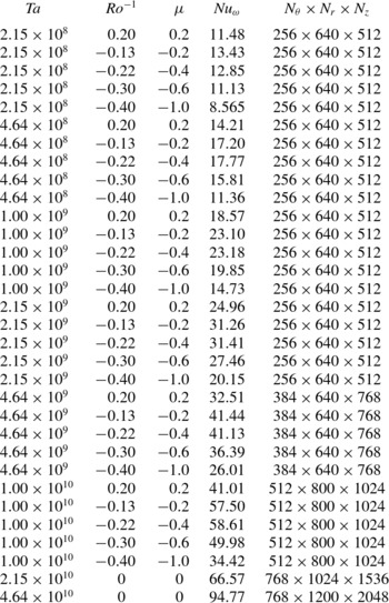
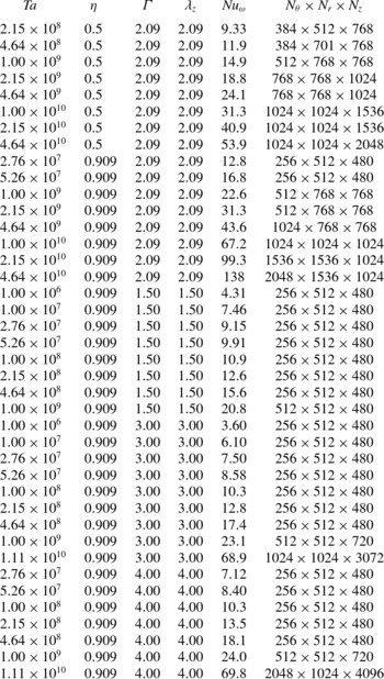
A second-order finite-difference code was used with fractional time integration. The code was parallelized using hybrid OpenMP and MPI-slab decomposition. Simulations were run on local clusters and on the supercomputer CURIE (thin nodes) using a maximum of 8192 cores. Details about the code can be found in Verzicco & Orlandi (Reference Verzicco and Orlandi1996) and in Ostilla-Mónico et al. (Reference Ostilla-Mónico, Stevens, Grossmann, Verzicco and Lohse2013). The explored parameter space from previous work (Ostilla-Mónico et al.
Reference Ostilla-Mónico, Stevens, Grossmann, Verzicco and Lohse2013, Reference Ostilla-Mónico, van der Poel, Verzicco, Grossmann and Lohse2014b
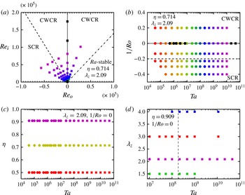
) was extended through further simulations. Figure 1 shows the parameter space explored in this manuscript. Circles show simulations of a ‘full’ geometry, i.e. a complete cylinder and with
 ${\rm\Gamma}=2{\rm\pi}$
. Following the work of Brauckmann & Eckhardt (Reference Brauckmann and Eckhardt2013a
), the simulations with the largest
 $\mathit{Ta}$
were performed on ‘reduced’ geometries to reduce computational costs, and these are indicated as squares in the plots. The idea is that instead of simulating the whole cylinder, a cylinder wedge with rotational symmetry of order
 $n_{sym}$
is considered. The aspect ratio was also reduced to
 ${\rm\Gamma}=2{\rm\pi}/3$
, accommodating a single vortex pair with the wavelength
 ${\it\lambda}_{z}=2{\rm\pi}/3=2.09$
. The vortical wavelength remains the same, although there is a single vortex instead of the three vortex pairs having also the wavelength
 ${\it\lambda}_{z}=2{\rm\pi}/3$
. Other vortical wavelengths were also simulated using reduced geometries for
 ${\it\eta}=0.909$
. We note that the aspect ratio
 ${\rm\Gamma}$
is a geometrical control parameter, but
 ${\it\lambda}_{z}$
is a response of the system, which depends both on
 ${\rm\Gamma}$
and on the amount of vortex pairs which fit in the system. They are related by
 ${\it\lambda}_{z}={\rm\Gamma}/n$
, where
 $n$
is the amount of vortex pairs which fit in the system. For all simulations axially periodic boundary conditions were used. Its consequences on the vortex wavelength are analysed in § 4. Further details on the numerical resolution can be found in table 1 in appendix A.
(a) Explored
 $(\mathit{Re}_{i},\mathit{Re}_{o})$
parameter space for
 ${\it\eta}=0.714$
,
 ${\it\lambda}_{z}=1.04$
. (b) Same as (a), but now in the
 $(\mathit{Ta},1/\mathit{Ro})$
parameter space. In both panels the solid line indicates pure inner cylinder rotation, the dot-dashed line indicates the Rayleigh stability criterium, while the dashed line indicates the asymptotic position of optimum transport in experiments, i.e.
 $\mathit{Ro}^{-1}=-0.20$
. The Rayleigh-stability line lies outside the top right panel, at
 $\mathit{Ro}^{-1}=0.83$
. These lines divide the parameter space into the Rayleigh-stable zone, the co-rotating or weakly counter-rotating regime (CWCR) and the strongly counter-rotating regime (SCR). (c) Explored
 $(\mathit{Ta},{\it\eta})$
parameter space for
 $\mathit{Ro}^{-1}=0$
,
 ${\it\lambda}_{z}=1.04$
. (d) Explored
 $(\mathit{Ta},{\it\lambda}_{z})$
parameter space for
 $\mathit{Ro}^{-1}=0$
,
 ${\it\eta}=0.909$
. The dashed line indicates the cross-point of branches with different
 ${\it\lambda}_{z}$
in Martinez-Arias et al. (Reference Martinez-Arias, Peixinho, Crumeyrolle and Mutabazi2014). For (c,d), the same colour coding is maintained throughout the paper, in the online version. (a–d) Circles indicate simulations of the ‘full’ geometry, with three vortex pairs, while squares indicate simulations of ‘reduced’ geometries with forced rotational symmetry and one vortex pair.

2.3. Explored parameter space
Figure 1(a,b) show the parameter space explored for
 ${\it\eta}=0.714$
in both
 $(\mathit{Re}_{i},\mathit{Re}_{o})$
and
 $(\mathit{Ta},1/\mathit{Ro})$
to study the effects of outer cylinder rotation. For
 ${\it\eta}=0.714$
, reduced geometries simulate one sixth of the cylinder, i.e.
 $n_{sym}=6$
as used in Ostilla-Mónico et al. (Reference Ostilla-Mónico, van der Poel, Verzicco, Grossmann and Lohse2014b
). The chosen values of
 $\mathit{Ro}^{-1}$
include a co-rotating outer cylinder (
 $\mathit{Ro}^{-1}=0.20$
), a weakly counter-rotating outer cylinder (
 $\mathit{Ro}^{-1}=-0.13$
), counter-rotation near the asymptotic position of optimal transport,
 $\mathit{Ro}_{opt}^{-1}$
(
 $\mathit{Ro}^{-1}=-0.22$
), and two values of
 $\mathit{Ro}^{-1}$
in the strongly counter-rotating regime (
 $\mathit{Ro}^{-1}=-0.30$
and
 $\mathit{Ro}^{-1}=-0.40$
). No simulations were run in the Rayleigh-stable regime (i.e. when
 $r_{o}^{2}{\it\omega}_{o}>r_{i}^{2}{\it\omega}_{i}$
) as no evidence of turbulence was found in that regime up to
 $\mathit{Ta}\sim 10^{10}$
in Ostilla-Mónico et al. (Reference Ostilla-Mónico, Verzicco, Grossmann and Lohse2014c
).
In addition, to study the effects of geometry, i.e. both the radius ratio
 ${\it\eta}$
and the vortical wavelength
 ${\it\lambda}_{z}$
(controlled through the aspect ratio
 ${\rm\Gamma}$
), additional simulations were performed. Figure 1(c) shows that two additional radius ratios were simulated up to
 $\mathit{Ta}=4\times 10^{10}$
, one with a larger gap (
 ${\it\eta}=0.5$
) and one with a smaller gap (
 ${\it\eta}=0.909$
). For
 ${\it\eta}=0.5$
, one third of the cylinder (
 $n_{sym}=3$
) was simulated for
 $\mathit{Ta}$
larger than
 $10^{8}$
. This value of
 $n_{sym}$
for
 ${\it\eta}=0.5$
was shown not to affect the values of the torque obtained in the simulations in Brauckmann & Eckhardt (Reference Brauckmann and Eckhardt2013b
). For
 ${\it\eta}=0.909$
, one twentieth of the geometry (
 $n_{sym}=20$
) was used.
Figure 1(d) shows the simulations with varying vortical wavelength
 ${\it\lambda}_{z}$
done for
 ${\it\eta}=0.909$
and pure inner cylinder rotation. We chose
 ${\it\eta}=0.909$
as we expect the effects of the coherent structures, and thus of
 ${\it\lambda}_{z}$
, to be stronger for larger
 ${\it\eta}$
(see later §§ 4 and 5 for an explanation). The values of
 $\mathit{Ta}$
simulated are around the range where Martinez-Arias et al. (Reference Martinez-Arias, Peixinho, Crumeyrolle and Mutabazi2014) have experimentally observed the crossing of different branches in
 $Nu_{{\it\omega}}(\mathit{Ta})$
and also coincides with the onset of the ‘ultimate’ regime.
2.4. Non-dimensionalization
The following non-dimensionalizations will be used: as the flow is simulated in a rotating frame, the outer cylinder is stationary, and the system has an unique velocity scale, equal to
 $U\equiv r_{i}({\it\omega}_{i}^{\ell }-{\it\omega}_{o}^{\ell })$
in the laboratory frame. All velocities are non-dimensionalized using
 $U$
, i.e.
 $\tilde{\boldsymbol{u}}=\boldsymbol{u}/U$
. The gap width
 $d$
is the characteristic length scale, and thus used for normalizing distances.
We define the normalized (non-dimensional) distance from the inner cylinder
 $\tilde{r}=(r-r_{i})/d$
and the normalized height
 $\tilde{z}=z/d$
. We furthermore define the time- and azimuthally averaged velocity fields as
 $$\begin{eqnarray}\bar{\tilde{\boldsymbol{u}}}(r,z)=\langle \tilde{\boldsymbol{u}}({\it\theta},r,z,t)\rangle _{{\it\theta},t},\end{eqnarray}$$
where
 $\langle {\it\phi}(x_{1},x_{2},\dots ,x_{n})\rangle _{x_{i}}$
indicates averaging of the field
 ${\it\phi}$
with respect to
 $x_{i}$
. As mentioned previously, the torque is non-dimensionalized as an angular velocity ‘Nusselt’ number (EGL07), defined as
 $Nu_{{\it\omega}}=T/T_{pa}$
, where
 $T_{pa}$
is the torque in the purely azimuthal flow. The torque is calculated from the radial derivative of
 $\langle \bar{\tilde{{\it\omega}}}\rangle _{z}$
at the inner and outer cylinders. The simulations are run in time until the respective values are equal within 1 %. The torque is then taken as the average value of the inner and outer cylinder torques. Therefore, the error due to finite time statistics is smaller than 1 %.
From here on, for convenience we will drop the overhead tilde on all non-dimensionalized variables.
2.5. Structure of paper
The organization of the paper is as follows. In § 3, we analyse the effect of rotating the outer cylinder. This is followed by § 4, where we study the influence of
 ${\it\eta}$
, and note an analogy between the effects of smaller
 ${\it\eta}$
and larger
 $\mathit{Ro}^{-1}$
. In § 5, we consider the effects of the last parameter, the vortical wavelength
 ${\it\lambda}_{z}$
. We finish in § 6 with a summary of the results and an outlook for future work.
3. The effect of outer cylinder rotation or the inverse Rossby number dependence
In this section we will study the effect of the Coriolis force (
 $\mathit{Ro}^{-1}$
), originating from the rotation of the outer cylinder, on the scaling of
 $Nu_{{\it\omega}}(\mathit{Ta})$
with
 $\mathit{Ta}$
and, more specifically, the effect of
 $\mathit{Ro}^{-1}$
on the transition to the ultimate regime. Depending on the value of
 $\mathit{Ro}^{-1}$
, two distinct regimes will be identified: first a co- and weakly counter-rotating
 $\mathit{Ro}^{-1}$
range, denoted from here on as the CWCR regime, and second the strongly counter-rotating
 $\mathit{Ro}^{-1}$
range, denoted from here on as SCR regime. The CWCR regime is found when the outer cylinder either is at rest, co-rotates with the inner cylinder, or slowly counter-rotates. The counter-rotation must be slow enough such that no Rayleigh-stable zones are generated in the bulk of the flow. In this CWCR regime the Coriolis force is balanced through the bulk gradient of
 ${\it\omega}$
. This can be derived from a large-scale balance in the
 ${\it\theta}$
-component of the velocity in (2.2). In summary, the nonlinear term
 $u_{r}(\partial _{r}u_{{\it\theta}}+u_{r}u_{{\it\theta}}/r)$
and the Coriolis force term
 $-u_{r}\mathit{Ro}^{-1}$
balance each other out on average (cf. Ostilla-Mónico et al.
Reference Ostilla-Mónico, Stevens, Grossmann, Verzicco and Lohse2013 for the full derivation). This results in a linear relationship between
 $\mathit{Ro}^{-1}$
and
 $\partial _{r}\langle \bar{{\it\omega}}\rangle _{z}$
(Ostilla-Mónico et al.
Reference Ostilla-Mónico, Huisman, Jannink, van Gils, Verzicco, Grossmann, Sun and Lohse2014a
).
TC flow can be considered as being in the SCR regime, if the outer cylinder strongly counter-rotates and generates a Coriolis force which exceeds what the
 ${\it\omega}$
-gradient can balance. The threshold value of
 $\mathit{Ro}^{-1}$
corresponds to the flattest
 ${\it\omega}$
profile. This also is the value of
 $\mathit{Ro}^{-1}$
, for which
 $Nu_{{\it\omega}}(\mathit{Ro}^{-1})$
is found to be largest (van Gils et al.
Reference van Gils, Huisman, Grossmann, Sun and Lohse2012; Ostilla-Mónico et al.
Reference Ostilla-Mónico, Stevens, Grossmann, Verzicco and Lohse2013), denoted henceforth as
 $\mathit{Ro}_{opt}^{-1}$
. In this regime the turbulent plumes originating from the inner cylinder are not strong enough to overcome the stabilizing effect of the outer cylinder, and the flow is divided into two regions, a Rayleigh-stable region in the outer gap region, which plumes do not reach, and a Rayleigh-unstable region in the inner parts of the gap. For given Coriolis force, the relative sizes of these spatial regions depend on
 $\mathit{Ta}$
, as for a stronger driving (i.e. larger
 $\mathit{Ta}$
), the turbulence originating from the inner cylinder ‘pushes’ these zones more towards the outer cylinder. This may lead to switching between vortical states and jumps in global quantities as seen in Ostilla-Mónico et al. (Reference Ostilla-Mónico, Stevens, Grossmann, Verzicco and Lohse2013). The boundary between both regimes is at
 $\mathit{Ro}_{opt}^{-1}$
. Of course,
 $\mathit{Ro}_{opt}^{-1}$
depends on
 $\mathit{Ta}$
too, due to effect of viscosity in the Coriolis force balance (Ostilla-Mónico et al.
Reference Ostilla-Mónico, Stevens, Grossmann, Verzicco and Lohse2013), and only saturates to
 $\mathit{Ro}_{opt}^{-1}(\mathit{Ta}\rightarrow \infty )=-0.20$
for sufficiently high drivings of
 $\mathit{Ta}\sim 5\times 10^{8}$
and more (cf. figure 2(a,b) and Brauckmann & Eckhardt Reference Brauckmann and Eckhardt2013a
).
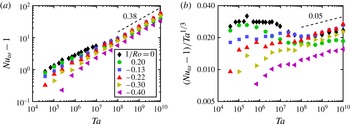
Figure 2 shows both
 $Nu_{{\it\omega}}-1$
and the compensated Nusselt number
 $(Nu_{{\it\omega}}-1)/\mathit{Ta}^{1/3}$
versus
 $\mathit{Ta}$
for
 ${\it\eta}=0.714$
and the six values of
 $\mathit{Ro}^{-1}$
studied. For the largest drivings (i.e.
 $\mathit{Ta}>10^{9}$
) all values of
 $\mathit{Ro}^{-1}$
reach the effective scaling law
 $Nu_{{\it\omega}}\sim \mathit{Ta}^{0.38}$
(with a different amplitude), similar to what was reported in the experiments by van Gils et al. (Reference van Gils, Huisman, Bruggert, Sun and Lohse2011). However, very different behaviour can be seen for
 $\mathit{Ta}<10^{9}$
, i.e. before the onset of the ultimate regime.
(a) The non-dimensional torque
 $Nu_{{\it\omega}}-1$
versus the driving, i.e. the Taylor number
 $\mathit{Ta}$
, for
 ${\it\eta}=0.714$
and six values of
 $\mathit{Ro}^{-1}$
. (b) The compensated Nusselt
 $(Nu_{{\it\omega}}-1)/\mathit{Ta}^{1/3}$
versus the driving
 $\mathit{Ta}$
for the same six values of
 $\mathit{Ro}^{-1}$
. The effective scaling law of
 $Nu_{{\it\omega}}\sim \mathit{Ta}^{0.38}$
is reached for all
 $\mathit{Ro}^{-1}$
at the highest drivings
 $\mathit{Ta}$
beyond about
 $10^{9}$
. However, the behaviour in the classical regime
 $\mathit{Ta}$
less than
 $10^{9}$
depends heavily on
 $\mathit{Ro}^{-1}$
. Before the onset of the ultimate regime, we observe a transitional
 $\mathit{Ta}$
regime ranging from about
 $10^{6}$
to about
 $10^{8}$
associated to the breakup of coherent structures for co-rotating and weakly counter-rotating cylinders (
 $-0.13\leqslant \mathit{Ro}^{-1}\leqslant 0.2$
). For more positive values of
 $\mathit{Ro}^{-1}$
this regime can be seen earlier, and is persistent for a larger
 $\mathit{Ta}$
range. For the strongly counter-rotating cases (
 $\mathit{Ro}^{-1}\leqslant -0.22$
), an effective local scaling exponent with
 ${\it\alpha}>{\textstyle \frac{1}{3}}$
is seen in the classical regime. This can be related to the interplay between Rayleigh-stable and Rayleigh-unstable regions.

In the CWCR regime (
 $\mathit{Ro}^{-1}\geqslant \mathit{Ro}_{opt}^{-1}=-0.20$
), the Coriolis force is reflected in the flow structure through the bulk gradient of
 ${\it\omega}$
, making it either flatter as in the case of weak counter-rotation, or steeper, as in the case of co-rotation (if the driving is sufficiently large). A consequence of the angular velocity gradient in the bulk is that large-scale structures can be weakened or even completely disappear in the CWCR regime. These changes in
 ${\it\omega}$
-gradient strongly affect the capability of plumes to ‘coordinate’ and form a large-scale wind, which in turn leads to an earlier (or later) onset of the sharp decrease in the local exponent
 ${\it\alpha}$
in the scaling law
 $(Nu_{{\it\omega}}-1)\sim \mathit{Ta}^{{\it\alpha}}$
associated with the breakdown of coherence, and the onset of time dependence in
 $Nu_{{\it\omega}}$
(Ostilla-Mónico et al.
Reference Ostilla-Mónico, van der Poel, Verzicco, Grossmann and Lohse2014b
).
For the case of co-rotating cylinders (
 $\mathit{Ro}^{-1}=0.20$
), this happens when the system enters the so-called ‘wavelet’ regime, characterized by moving waves in the boundary regions between a pair of Taylor vortices (Andereck et al.
Reference Andereck, Dickman and Swinney1983, Reference Andereck, Liu and Swinney1986). These waves move with different speeds, and as a consequence this regime is not stationary in any reference frame. This regime only persists for a small range of
 $\mathit{Ta}$
, and eventually all remnants of Taylor vortices vanish. Axial dependence of the flow structure is almost completely lost, even at
 $\mathit{Ta}$
as low as
 $\mathit{Ta}\approx 5\times 10^{7}$
. Unlike the case of
 $\mathit{Ro}^{-1}=0$
studied by Ostilla-Mónico et al. (Reference Ostilla-Mónico, van der Poel, Verzicco, Grossmann and Lohse2014b
), however, in this transitional regime, the large-scale rolls already completely vanished, but for
 $\mathit{Ro}^{-1}=0.20$
this does not immediately lead to the transition to the ultimate regime. After its sharp decrease,
 ${\it\alpha}$
does not exceed
 ${\textstyle \frac{1}{3}}$
. Instead, at a driving strength around
 $\mathit{Ta}\approx 10^{7}$
(coinciding with the disappearance of the structures), the local effective scaling exponent
 ${\it\alpha}$
has increased to
 ${\it\alpha}\approx {\textstyle \frac{1}{3}}$
, and then stops growing. Only if
 $\mathit{Ta}$
increases further and the shear in the boundary layers grows past a threshold, a shear-instability takes place, and the system transitions to the ultimate regime.
For the case of counter-rotating cylinders (i.e.
 $\mathit{Ro}^{-1}<0$
),
 ${\it\alpha}$
can locally grow beyond
 ${\it\alpha}={\textstyle \frac{1}{3}}$
in the classical regime. This is unexpected, as values of
 ${\it\alpha}$
larger than one third have been associated to the transition to turbulence of the boundary layers in the context of both RB convection (He et al.
Reference He, Funfschilling, Nobach, Bodenschatz and Ahlers2012b
), and TC flow with a stationary outer cylinder (Ostilla-Mónico et al.
Reference Ostilla-Mónico, van der Poel, Verzicco, Grossmann and Lohse2014b
). However, in this case, the shear in the boundary layers is too low so the boundary layers still stay laminar.
For counter-rotating cylinders, a wide range of flow configurations is available in the low-
 $\mathit{Ta}$
regime (Andereck et al.
Reference Andereck, Liu and Swinney1986). We can relate local steps in
 ${\it\alpha}$
to the switching between such flow configurations. The interplay between Rayleigh-stable and Rayleigh-unstable regions can also play a role. Larger drivings cause the Rayleigh-unstable region to grow, and thus to increase the transport. These two effects lead to larger increases in the non-dimensional torque than what is expected for pure inner cylinder rotation, and explain the large values of
 ${\it\alpha}$
seen.
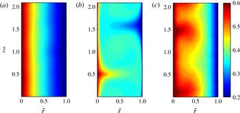
Contour plots of the azimuthally and time-averaged angular velocity field
 $\bar{{\it\omega}}$
for
 $\mathit{Ta}=10^{10}$
,
 ${\it\eta}=0.714$
and three values of
 $\mathit{Ro}^{-1}$
. (a) Corresponds to
 $\mathit{Ro}^{-1}=0.2$
(CWCR regime) and shows no traces of axial dependence. Plumes detach rapidly into the bulk, mix there strongly, and thus cannot form large-scale structures. (b) Corresponds to
 $\mathit{Ro}^{-1}=-0.22$
(
 ${\approx}\mathit{Ro}_{opt}^{-1}$
). The reduced plume mixing enables the formation of large-scale structures, and a strong signature of them can be seen in the averaged angular velocity field. (c) Corresponds to
 $\mathit{Ro}^{-1}=-0.40$
(SCR regime) and also shows some signatures of large-scale structures. However, these do not fully penetrate the gap but stop at the border to the Rayleigh-stable zones near the outer cylinder.

To further illustrate the effect of the Coriolis force on the large-scale structures, figure 3 presents a contour plot of
 $\bar{{\it\omega}}$
in the CWCR regime
 $\mathit{Ro}^{-1}=0.20$
, around the optimum
 $\mathit{Ro}^{-1}=-0.22\approx \mathit{Ro}_{opt}^{-1}$
and in the SCR regime
 $\mathit{Ro}^{-1}=-0.40$
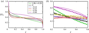
. Figure 4 shows the axially-averaged angular velocity profiles
 $\langle \bar{{\it\omega}}\rangle _{z}$
for
 ${\it\eta}=0.714$
and the six values of
 $\mathit{Ro}^{-1}$
simulated here. The large-scale structures cannot be seen in figure 3(a), which corresponds to
 $\mathit{Ro}^{-1}=0.20$
(co-rotating cylinders), but they are pronounced for the other two panels (
 $\mathit{Ro}^{-1}=-0.22$
and
 $\mathit{Ro}^{-1}=-0.40$
). As shown in figure 4, in the CWCR regime, the bulk sustains a large
 $\bar{{\it\omega}}_{z}$
gradient, and to accommodate for this, there is smaller
 $\bar{{\it\omega}}_{z}$
jump across the boundary layers. Plumes ejected from both cylinders can now mix easier when entering the bulk. As a consequence, the large-scale structures, which essentially consist of unmixed plumes, break up easier and thus do that for lower values of
 $\mathit{Ta}$
. For this reason they have completely vanished in figure 3(a).
If we now decrease
 $\mathit{Ro}^{-1}$
, the profile becomes flatter. The effect of this is visible in figure 3(b) showing
 $\bar{{\it\omega}}$
for
 $\mathit{Ro}^{-1}=-0.22$
. It can be seen from figure 4 that this value of
 $\mathit{Ro}^{-1}$
corresponds to the flattest
 ${\it\omega}$
-profile available, and it is also the closest to the experimental optimum transport
 $\mathit{Ro}_{opt}^{-1}(\mathit{Ta}\rightarrow \infty )=-0.20$
. A very marked signature of the large-scale structure on
 $\bar{{\it\omega}}$
can be seen. This is because a very flat
 $\bar{{\it\omega}}$
profile will sustain a large
 $\bar{{\it\omega}}$
jump across the boundary layer, and thus plumes detach less violently into the bulk, thus stabilizing the large-scale structures. Therefore, we can relate the flatness of the
 $\bar{{\it\omega}}$
-profile to the strength of the large-scale circulation, and this in turn can be related to the optimum in
 $Nu_{{\it\omega}}(\mathit{Ro}^{-1})$
. As mentioned in Brauckmann & Eckhardt (Reference Brauckmann and Eckhardt2013b
), optimum transport coincides with the strongest mean circulation. Plumes travel faster from one cylinder to the other when the large-scale circulation is strongest, and thus more angular momentum is transferred. We also highlight that the signature of the large-scale structures on the mean azimuthal flow remains even in the ultimate regime, and is also seen in experiment at
 $\mathit{Ta}\sim 10^{12}$
(Huisman et al.
Reference Huisman, van der Veen, Sun and Lohse2014). Thus, in general the vanishing of the rolls appears to be independent from the transition to the ultimate regime. Only in the special case of pure inner cylinder rotation these two effects coincidentally occur at the same
 $\mathit{Ta}$
.
In figure 3(b), we can see that once the Coriolis force is sufficiently large, the vortices cannot fully penetrate the domain. Near the outer cylinder, the flow is predominantly Rayleigh stable. Rayleigh-stable zones are well mixed, as transport here happens through intermittent turbulent bursts, instead of convective transport by plumes and vortices (Brauckmann & Eckhardt Reference Brauckmann and Eckhardt2013b
). Thus, in Rayleigh-stable regions, no rolls can be seen in the averaged fields. The effect of the neutral surface can also be observed in the averaged
 ${\it\omega}$
profiles (cf. figure 4). The two simulated cases in the SCR regime (
 $\mathit{Ro}^{-1}=-0.30$
and
 $\mathit{Ro}^{-1}=-0.40$
) show an outer cylinder boundary layer which with more and more negative
 $\mathit{Ro}^{-1}$
extends deeper into the flow, and the distinction from the bulk is blurred away.
(a) Azimuthally, axially and time-averaged and non-dimensionalized angular velocity profiles
 $\langle \bar{{\it\omega}}\rangle _{z}$
for
 ${\it\eta}=0.714$
,
 $\mathit{Ta}=10^{10}$
, and six values of
 $\mathit{Ro}^{-1}$
. For co- and weakly counter-rotating cylinders, we see that the bulk
 $\bar{{\it\omega}}$
profiles become flatter as
 $\mathit{Ro}^{-1}$
becomes more negative. Thus, the angular velocity difference, which the plumes encounter when detaching from the boundary layer and entering the bulk, is larger for more negative
 $\mathit{Ro}^{-1}$
. (b) Enlarged view of the bulk region of (a). LDA data from experiments from (van Gils et al.
Reference van Gils, Huisman, Grossmann, Sun and Lohse2012), for which
 $\mathit{Re}_{i}-\mathit{Re}_{o}=10^{6}$
have been superimposed. Note the good agreement between both datasets for values of
 $\mathit{Ro}^{-1}$
in the CWCR regime, while discrepancies exist for values of
 $\mathit{Ro}^{-1}$
around the optimum and in the SCR regime. This is attributed to the axial dependence of the profiles, which exists in this regime, see figure 3, and as experimental data is measured at fixed height, while numerical data are axially averaged.

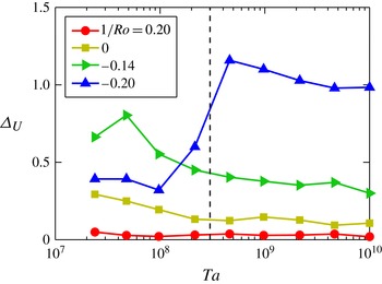
To further disentangle the effect of axial dependence and the transition to the ultimate regime we show the loss of axial dependence characterized by a special spread measure
 ${\rm\Delta}_{U}$
as a function of the driving
 $\mathit{Ta}$
in figure 5. Here
 ${\rm\Delta}_{U}$
is defined as
 ${\rm\Delta}_{U}=(\max _{z}(\bar{u_{{\it\theta}}}(r_{a},z))-\min _{z}(\bar{u_{{\it\theta}}}(r_{a},z)))/\langle \bar{u_{{\it\theta}}}(r_{a},z)\rangle _{z}$
, with
 $r_{a}$
, the mid-gap, defined as
 $r_{a}=r_{i}+d/2$
, the arithmetic mean of the inner and outer cylinder radii. When measuring the axial spread, the velocity is averaged in time, and azimuthally, as the flow is homogeneous in the azimuthal direction. As stated previously, for co-rotating cylinders, the axial dependence disappears for low drivings corresponding to those in the transitional regime, and associated to the appearance of the ‘wavelet’ states. For counter-rotating cylinders, a sharp jump in
 ${\rm\Delta}_{U}$
can be noticed. This is due to
 ${\rm\Delta}_{U}$
being measured at the mid-cylinder
 $\tilde{r}=\tilde{r}_{a}$
. For low drivings,
 $\tilde{r}_{a}$
is located in the Rayleigh-stable zones, and the flow is mixed better. As the driving increases, turbulence from the inner cylinder pushes the neutral surface, which divides the stable and unstable zones further towards the outer cylinder. As a consequence of this pushing,
 $\tilde{r}_{a}$
is no longer in the Rayleigh-stable zone, but instead in the Rayleigh-unstable zone. This zone is dominated by large-scale structures. This makes the axial dependence increase and provides more evidence that the vanishing of the Taylor rolls is only coincidental with the transition to the ultimate regime for pure inner cylinder rotation.
The axial velocity spread measure
 ${\rm\Delta}_{U}$
versus
 $\mathit{Ta}$
for the four values of
 $\mathit{Ro}^{-1}$
in the CWCR regime. The dashed line indicates the approximate value of
 $\mathit{Ta}$
where the flow transitions to the ultimate regime for all values of
 $\mathit{Ro}^{-1}$
, which was previously associated with the vanishing of the large-scale structures. For co-rotating cylinders (
 $\mathit{Ro}^{-1}=0.20$
), at
 $\mathit{Ta}$
as low as
 $\mathit{Ta}\approx 10^{7}$
no axial dependence is seen, well before the transition. For counter-rotating cylinders a sharp increase of the axial velocity spreading measure
 ${\rm\Delta}_{U}$
can be seen, which then slowly decreases with increasing
 $\mathit{Ta}$
. The sharp increase in
 ${\rm\Delta}_{U}$
can be associated to the growth of the Rayleigh-unstable zones. For low
 $\mathit{Ta}$
, the mid-gap is in a Rayleigh-stable zone mixed by bursts, while for large
 $\mathit{Ta}$
, the mid-gap is in a Rayleigh-unstable zone, dominated by rolls leading to a strong height dependence. The large axial spreads explain the discrepancies when comparing (axially averaged) DNS data to experimental data measured at a fixed height.

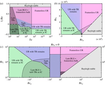
As mentioned previously, the value of
 $\mathit{Ro}_{opt}^{-1}$
, and thus of the border between the CWCR and the SCR regimes depends on
 $\mathit{Ta}$
. This is summarized in figure 6, which shows the approximate division between the different flow regimes explored in this paper in both the
 $(\mathit{Ta},\mathit{Ro}^{-1})$
and the
 $(\mathit{Re}_{i},\mathit{Re}_{o})$
parameter spaces, both for
 ${\it\eta}=0.714$
. Note that
 $\mathit{Ro}_{opt}^{-1}$
, and thus the division between the regimes, can be seen to saturate for
 $\mathit{Ta}\sim 5\times 10^{8}$
, when driving is large enough, and the mean
 $\bar{{\it\omega}}(r)$
profile at
 $\mathit{Ro}_{opt}^{-1}$
is completely flat.
Transition between different regimes in the
 $(\mathit{Ta},\mathit{Ro}^{-1})$
(a) and
 $(\mathit{Re}_{i},\mathit{Re}_{o})$
(b,c) parameter spaces for
 ${\it\eta}=0.714$
. The hollow circles indicate the location of optimal transport, and serve as an indication of the movement of the division between CWCR (blueish and reddish) and SCR (greenish) regimes with
 $\mathit{Ta}$
. In both DNS and experiments,
 $\mathit{Ro}_{opt}^{-1}$
reaches an asymptotic value for
 $\mathit{Ta}>5\times 10^{8}$
. For larger
 ${\it\eta}$
(smaller gap), this separation line moves towards smaller
 $\mathit{Ro}^{-1}$
. For
 $\mathit{Ta}\lesssim 10^{7}$
, we have the rich variety of different states of Andereck et al. (Reference Andereck, Liu and Swinney1986), not detailed in this diagram. This region appears explicitly in (a) as ‘lam TRs’ and ‘lam TRs at IC’, but is not shown in the other two due to the axes used. Abbreviations: boundary layer (BL), Taylor rolls (TR), ultimate regime (UR) and inner cylinder (IC).

Finally, to further justify the division of the flow into the CWCR and the SCR regimes with decreasing inverse Rossby number
 $\mathit{Ro}^{-1}$
, we can quantify the distribution of Rayleigh-stable and Rayleigh-unstable zones as a function of
 $\mathit{Ro}^{-1}$
. This is done by looking at the PDF of
 $\tilde{r}_{N}$
, i.e. the collection of points outlining the neutral surface
 $\tilde{r}_{N}=\tilde{r}_{N}(t,{\it\theta},z)$
. This is, the border between Rayleigh-stable outer gap range and the Rayleigh-unstable inner gap parts, and given as the points for which
 ${\it\omega}(t,{\it\theta},z,\tilde{r}_{N})=0$
in the laboratory (non-rotating) frame. For counter-rotating cylinders, the neutral surface defines the instantaneous border between Rayleigh-stable and Rayleigh-unstable zones. For co-rotating cylinders, the neutral line does not exist, and the whole flow is either Rayleigh stable or Rayleigh unstable. In principle, the neutral surface might be fragmented, and thus the position of
 $\tilde{r}_{n}$
multivalued. However, this is usually not the case. When taking the ensemble, all values are considered, as this does not change the PDFs significantly.
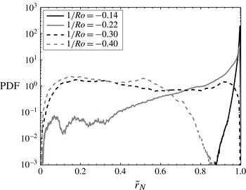
Figure 7 shows the PDFs of
 $\tilde{r}_{N}$
calculated for the four negative values of
 $\mathit{Ro}^{-1}$
at the largest driving simulated here. The difference between the two regimes can clearly be noticed. In the CWCR regime and near the optimum, the border between the zones is located very closely to the outer cylinder, which means that almost all the domain is Rayleigh unstable and dominated by plumes or rolls. In the SCR regime, the border between the zones is pushed closer towards the inner cylinder, and Rayleigh-stable zones appear all over the gap. For the most negative simulated value of
 $\mathit{Ro}^{-1}$
, i.e.
 $\mathit{Ro}^{-1}=-0.40$
, the areas near the outer cylinder are permanently Rayleigh stable, and transport occurs in intermittent bursts which mix this zone well. This causes the partial disappearance of axial dependence seen in figure 3(b).
DNS results for the PDFs of the radial position
 $\tilde{r}_{N}$
of the neutral surface, at the border between Rayleigh-stable and Rayleigh-unstable regions, for the four simulated negative values of
 $\mathit{Ro}^{-1}$
(i.e. for counter-rotating cylinders) for
 $\mathit{Ta}=10^{10}$
. For
 $\mathit{Ro}^{-1}=-0.14$
(CWCR) and
 $\mathit{Ro}^{-1}=-0.22$
(close to the optimum), the PDFs show that the destabilizing action of the inner cylinder causes the Rayleigh-stable regions to be confined only very closely to the outer cylinder. For
 $\mathit{Ro}^{-1}=-0.22$
we can begin to see a limited amount of Rayleigh-stable zones in the whole domain, as
 $-0.22$
is slightly more negative than
 $\mathit{Ro}_{opt}^{-1}$
. For
 $\mathit{Ro}^{-1}=-0.30$
(SCR), the stabilization due to the Coriolis force increases, and the border between the regions can be anywhere in the gap, indicating a mixture of stable and unstable zones everywhere in the gap. Finally, for
 $\mathit{Ro}^{-1}=-0.40$
(also SCR), the border between both zones never gets close to the outer cylinder. For this case, the portion of the gap width with
 $\tilde{r}>0.84$
is always Rayleigh stable.

4. The effect of radius ratio or the
 ${\it\eta}$
-dependence

In the previous section we showed that for
 ${\it\eta}=0.714$
the transition to the ultimate regime and the vanishing of the rolls only (incidentally) co-occur at the same
 $\mathit{Ta}$
for pure inner cylinder rotation. Flatter bulk
 ${\it\omega}$
-profiles result in stronger large-scale structures, and steeper bulk
 ${\it\omega}$
-profiles result in weaker large-scale structures which vanish at
 $\mathit{Ta}\sim 10^{6}$
. Now we will show that we can modify the
 $\bar{{\it\omega}}(r)$
profile in the bulk not only by varying the Coriolis force, but also by changing the radius ratio
 ${\it\eta}$
(or the gap width). In this section, we will thus analyse the influence of
 ${\it\eta}$
, to understand whether the co-occurrence of the vanishing large scales and the boundary-layer transition observed for pure inner cylinder rotation is just a coincidence seen in the case
 ${\it\eta}=0.714$
.
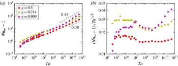
Figure 8 shows both the Nusselt number and the compensated Nusselt number plotted as a function of
 $\mathit{Ta}$
for the three values of
 ${\it\eta}$
simulated. As seen in Ostilla-Mónico et al. (Reference Ostilla-Mónico, Huisman, Jannink, van Gils, Verzicco, Grossmann, Sun and Lohse2014a
) for
 ${\it\eta}=0.714$
(and now also for
 ${\it\eta}=0.909$
), the flow undergoes a structural transition at around
 $\mathit{Ta}\approx 3\times 10^{6}$
, where the local exponent
 ${\it\alpha}$
of the effective scaling law
 $\mathit{Nu}\sim \mathit{Ta}^{{\it\alpha}}$
rapidly decreases. This is associated with the breakdown of coherence in the flow and the onset of time-dependence in the Nusselt number. For
 ${\it\eta}=0.714$
and
 ${\it\eta}=0.909$
, the effective exponent
 ${\it\alpha}$
begins to increase again after this breakdown. We can say that the flow transitions to the ultimate regime once
 ${\it\alpha}>{\textstyle \frac{1}{3}}$
, and this happens at about
 $\mathit{Ta}\approx 3\times 10^{8}$
. This
 $\mathit{Ta}$
value coincides with the experimentally observed value for the transition to the ultimate regime for
 ${\it\eta}=0.909$
(cf. Ravelet et al.
Reference Ravelet, Delfos and Westerweel2010).
For
 ${\it\eta}=0.5$
a different behaviour can be seen. After the breakdown of coherence, the transitional regime with
 ${\it\alpha}\approx {\textstyle \frac{1}{3}}$
goes on for three decades in
 $\mathit{Ta}$
, up to
 $\mathit{Ta}\approx 10^{10}$
(last three data points of the panel). An increase in
 ${\it\alpha}$
only happens for the last three data points, with
 $\mathit{Ta}>10^{10}$
. This might be the beginning of the transition to the ultimate regime, observed at about that value of
 $\mathit{Ta}$
in the experiments by Merbold et al. (Reference Merbold, Brauckmann and Egbers2013). We emphasize that the behaviour of the
 $Nu_{{\it\omega}}(\mathit{Ta})$
curve for
 ${\it\eta}=0.5$
is very similar to the one seen for
 ${\it\eta}=0.714$
and
 $\mathit{Ro}^{-1}=0.20$
(cf. figure 2), while the
 $Nu_{{\it\omega}}(\mathit{Ta})$
curve for
 ${\it\eta}=0.909$
is similar to that for
 $\mathit{Ro}^{-1}=-0.14$
and
 ${\it\eta}=0.714$
.
(a) The non-dimensional torque
 $Nu_{{\it\omega}}-1$
versus driving
 $\mathit{Ta}$
for pure inner cylinder rotation
 $\mathit{Ro}^{-1}=0$
and three values of
 ${\it\eta}$
. (b) The compensated Nusselt
 $(Nu_{{\it\omega}}-1)/\mathit{Ta}^{1/3}$
versus driving strength
 $\mathit{Ta}$
for the same three values of
 ${\it\eta}$
. The asymptotic effective scaling laws of the ultimate regime are reached for all values of
 ${\it\eta}$
at large enough drivings. For
 ${\it\eta}=0.909$
jumps in
 $Nu_{{\it\omega}}(\mathit{Ta})$
can be seen for the highest drivings (around
 $\mathit{Ta}\sim 10^{10}$
). These jumps cause the exponent of the local scaling laws to be around 0.44, and are caused by changes in the large-scale structures.

We thus can draw an analogy between the effects of varying
 ${\it\eta}$
and those of changing
 $\mathit{Ro}^{-1}$
. The larger the gap or the smaller
 ${\it\eta}$
is, the more the flow feels the curvature. This is reflected in an asymmetry between inner and outer cylinder, since the inner cylinder curvature becomes increasingly stronger relative to the outer cylinder curvature. Also the exact relationship
 ${\it\eta}^{-3}\partial _{r}\langle {\it\omega}\rangle |_{o}=\partial _{r}\langle {\it\omega}\rangle |_{i}$
(cf. van Gils et al.
Reference van Gils, Huisman, Grossmann, Sun and Lohse2012) must hold in both boundary layers due to the
 $r$
-independence of the angular velocity current
 $J^{{\it\omega}}=r^{3}(\langle u_{r}{\it\omega}\rangle _{z,{\it\theta},t}-{\it\nu}\partial _{r}\langle {\it\omega}\rangle _{z,{\it\theta},t})$
(EGL07). For
 ${\it\eta}=0.5$
we have
 ${\it\eta}^{-3}=8$
and the
 ${\it\omega}$
-slope at the inner cylinder is eight-fold steeper than the outer cylinder
 ${\it\omega}$
-slope. Thus, the inner–outer asymmetry is expected to become much more dominant for
 ${\it\eta}=0.5$
in comparison with
 ${\it\eta}=0.714$
(
 ${\it\eta}^{-3}=2.75$
) as well as
 ${\it\eta}=0.909$
(
 ${\it\eta}^{-3}=1.331$
), for which it is hardly visible anymore.
While the inner and outer cylinder boundary layers extend into the bulk equally for pure inner cylinder rotation (cf. Ostilla-Mónico et al.
Reference Ostilla-Mónico, Huisman, Jannink, van Gils, Verzicco, Grossmann, Sun and Lohse2014a
), the jump of
 ${\it\omega}$
in the boundary layers is much larger in the inner cylinder as compared with the outer cylinder due to the different slopes and equal extents. Therefore, the plumes are highly asymmetric, and smaller drivings
 $\mathit{Ta}$
break up the ‘plume conveyor belts’, which form the large-scale structures seen in the time-averaged azimuthal velocity. On top of this plume asymmetry, originating from the boundary layers, a larger curvature has an effect on the bulk. The underlying
 $\bar{{\it\omega}}(r)$
profile is less flat, and thus the drop in angular velocity inside the bulk is the larger the smaller the value of
 ${\it\eta}$
is.
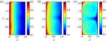
Both effects can be appreciated in figure 9, which shows contour plots of the azimuthally and time-averaged angular velocity
 $\bar{{\it\omega}}$
at
 $\mathit{Ta}=10^{10}$
for the three simulated values of
 ${\it\eta}$
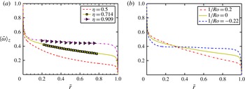
. This also explains figure 10(a), where the now also axially averaged angular velocity
 $\langle \bar{{\it\omega}}\rangle _{z}$
is shown for the same three values of
 ${\it\eta}$
. For comparison, figure 10(b) shows three profiles of
 $\langle \bar{{\it\omega}}\rangle _{z}$
in the CWCR regime for
 ${\it\eta}=0.714$
.
Contour plots of the azimuthally and time-averaged angular velocity field
 $\bar{{\it\omega}}$
for
 $\mathit{Ta}=10^{10}$
and
 $\mathit{Ro}^{-1}=0$
and three values of
 ${\it\eta}$
: (a)
 ${\it\eta}=0.5$
, (b)
 ${\it\eta}=0.714$
and (c)
 ${\it\eta}=0.909$
. The colour scale has been shifted in order to account for the different bulk angular velocities at different
 ${\it\eta}$
. Almost no axial dependence can be noticed for
 ${\it\eta}=0.5$
, while it is still very marked for
 ${\it\eta}=0.909$

(a) Axially averaged angular velocity profiles
 $\langle \bar{{\it\omega}}\rangle _{z}$
for
 ${\it\eta}=0.5$
,
 ${\it\eta}=0.714$
and
 ${\it\eta}=0.909$
at moderate driving
 $\mathit{Ta}=10^{10}$
and
 $\mathit{Ro}^{-1}=0$
. Solid lines are DNS data, while squares and triangles correspond to LDA data from experiments (
 $\mathit{Ta}=1.51\times 10^{12}$
for
 ${\it\eta}=0.714$
and
 $\mathit{Ta}=1.1\times 10^{11}$
for
 ${\it\eta}=0.909$
, from Ostilla-Mónico et al.
Reference Ostilla-Mónico, Huisman, Jannink, van Gils, Verzicco, Grossmann, Sun and Lohse2014a
). A larger decrease of
 ${\it\omega}$
across the bulk can be seen for
 ${\it\eta}=0.5$
. The angular velocity in the bulk also deviates more from
 ${\it\omega}=0.5$
, the expected value in the limit case of
 ${\it\eta}\rightarrow 1$
(plane Couette flow). (b) Axially-averaged angular velocity profiles
 $\langle \bar{{\it\omega}}\rangle _{z}$
for
 ${\it\eta}=0.714$
, and three values of
 $\mathit{Ro}^{-1}$
in the CWCR regime. The analogy between the effects of
 ${\it\eta}$
and
 $\mathit{Ro}^{-1}$
on
 $\bar{{\it\omega}}(\tilde{r})$
can be clearly seen.

The analogy between the effect of
 ${\it\eta}$
and the effect of
 $\mathit{Ro}^{-1}$
on
 ${\it\omega}(\tilde{r})$
is also demonstrated in figure 10. The rolls are weak for
 ${\it\eta}=0.5$
, as they are weak for co-rotating cylinders, and the rolls are strongest for
 ${\it\eta}=0.909$
and for
 $\mathit{Ro}^{-1}\approx \mathit{Ro}_{opt}^{-1}$
. This also explains why, for large enough
 $\mathit{Ta}$
,
 $Nu_{{\it\omega}}$
is highest at a given
 $\mathit{Ta}$
for the largest
 ${\it\eta}$
. However, the analogy is not perfect. For pure inner cylinder rotation, i.e. for
 $\mathit{Ro}^{-1}=0$
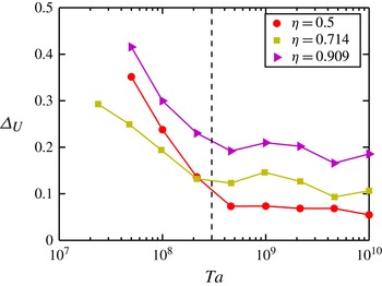
the wide variety of flow states seen in Andereck et al. (Reference Andereck, Dickman and Swinney1983) and Andereck et al. (Reference Andereck, Liu and Swinney1986) is greatly reduced. The system essentially goes from Taylor vortex flow to modulated Taylor vortex flow to finally turbulent Taylor vortex flow. It does not undergo transitions to different states (such as e.g. the ‘wavelet’ state), and thus the rolls do not vanish for the lower drivings at which this happens in co-rotating cylinders. This can be seen in figure 11, which shows the measure
 ${\rm\Delta}_{U}$
for the axial velocity spread as function of
 $\mathit{Ta}$
. With increased driving, the rolls progressively lose importance until
 $\mathit{Ta}$
reaches a value of
 $\mathit{Ta}\approx 3\times 10^{8}$
. However, the effect of
 ${\it\eta}$
, and thus of the cylinder wall curvature on the
 ${\it\omega}$
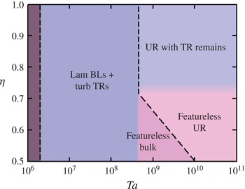
profiles can be clearly noticed in the residual axial dependence and behaves as expected from the analogy. The behaviour of the transition to the ultimate regime and associated subregimes is summarized in figure 12, which is analogous to figure 6, but now for the
 $(\mathit{Ta},{\it\eta})$
parameter space explored.
The measure
 ${\rm\Delta}_{U}$
for the axial velocity spread versus
 $\mathit{Ta}$
for the three values of
 ${\it\eta}$
simulated. A decrease in axial dependence can be seen for all values of
 ${\it\eta}$
around
 $\mathit{Ta}\approx 10^{8}$
, unlike what was seen for varying
 $\mathit{Ro}^{-1}$
, where the
 $\mathit{Ta}$
at which the decrease of axial dependence took place is
 $\mathit{Ro}^{-1}$
dependent. However, the residual axial spread at the largest drivings increases with increasing
 ${\it\eta}$
, as we would expect from the analogy between decreasing
 $\mathit{Ro}^{-1}$
and increasing
 ${\it\eta}$
.

Transition between different regimes in the
 $(\mathit{Ta},{\it\eta})$
parameter space for pure inner cylinder rotation
 $\mathit{Ro}^{-1}=0$
. The transition to the ultimate regime occurs at a higher
 $\mathit{Ta}$
for smaller
 ${\it\eta}$
(wider gap), while the vanishing of the large scale structures occurs at around the same
 $\mathit{Ta}$
for
 $0.5<{\it\eta}<0.714$
. Remains of the Taylor rolls can only be seen for large
 ${\it\eta}$
, i.e. smaller gap. Abbreviations: boundary layer (BL), Taylor rolls (TR), ultimate regime (UR).

Finally, one may ask the question of why the onset of the ultimate regime happens at a much higher
 $\mathit{Ta}$
for
 ${\it\eta}=0.5$
than for the two other values of
 ${\it\eta}$
studied. For
 ${\it\eta}=0.714$
, the transition seems to set in for the same value of
 $\mathit{Ta}$
independently of
 $\mathit{Ro}^{-1}$
. A factor of 10 increase in shear in the boundary layers is required for the boundary layer instability to occur and the ultimate regime to set in. Convex curvature is known to produce a stabilizing effect on boundary layers (Görtler Reference Görtler1940a
; Muck, Hoffmann & Bradshaw Reference Muck, Hoffmann and Bradshaw1985), and this will have a more significant effect on the inner cylinder for
 ${\it\eta}=0.5$
than for the larger
 ${\it\eta}$
. On the other hand we might expect that the destabilizing effect of concave curvature (Görtler Reference Görtler1940b
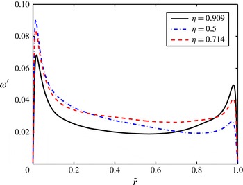
; Hoffmann, Muck & Bradshaw Reference Hoffmann, Muck and Bradshaw1985) would also play a role in accelerating the transition. Due to the boundary-layer asymmetry, however, the outer boundary layer is much more ‘quiet’, and has fewer fluctuations. This also delays the transition, and can be seen in figure 13, which shows the root mean square (r.m.s.) fluctuations of the angular velocity
 ${\it\omega}^{\prime }=\langle \langle {\it\omega}^{2}\rangle _{t,{\it\theta}}-\bar{{\it\omega}}^{2}\rangle _{z}^{1/2}$
, for
 $\mathit{Ta}=10^{9}$
and the three values of
 ${\it\eta}$
simulated. The levels of fluctuations at the outer cylinder are significantly reduced for
 ${\it\eta}=0.5$
when compared with the other values of
 ${\it\eta}$
. Finally, the large gradient of angular velocity sustained in the bulk will also reduce the shear in the outer cylinder, as the bulk angular velocity is smaller for
 ${\it\eta}=0.5$
. Thus, a combination of reduced fluctuations, stabilizing effect due to curvature at the inner cylinder, and reduced shear due to bulk angular velocity gradients is causing the delayed transition.
Root mean square (r.m.s.) profiles of the angular velocity fluctuations,
 ${\it\omega}^{\prime }(\tilde{r})$
, at
 $\mathit{Ta}=10^{9}$
and
 $\mathit{Ro}^{-1}=0$
for the three
 ${\it\eta}$
values simulated here. The boundary layer asymmetry causes the fluctuations to be strongly reduced at the outer cylinder for
 ${\it\eta}=0.5$
, as compared with those at the inner cylinder.

5. Dependence on number and size of rolls
Finally, we will quantify how the torque depends on the number and the size of the rolls, i.e. the vortical wavelength. The wavelength of a roll
 ${\it\lambda}_{z}$
is restricted to the values
 ${\it\lambda}={\rm\Gamma}/n$
, where
 $n$
is a strictly positive integer. For all simulations in this paper,
 $n=1$
, and thus
 ${\it\lambda}={\rm\Gamma}$
. This is not necessarily always the case,
 $n$
is a response of the system, and if
 ${\rm\Gamma}$
is large enough, i.e. the system can accommodate more than one vortex pair,
 $n$
can take several values depending on how the final state of the system is reached. Brauckmann & Eckhardt (Reference Brauckmann and Eckhardt2013a
) showed that for
 ${\it\eta}=0.714$
, the ‘optimal’ vortex wavelength, i.e. the vortex wavelength
 ${\it\lambda}_{z}$
which corresponds to a maximum
 $Nu_{{\it\omega}}$
, increased when comparing
 $Nu_{{\it\omega}}({\it\lambda}_{z})$
for two Taylor numbers, one in the Taylor vortex regime and another in the turbulent Taylor vortex regime. For the higher
 $\mathit{Ta}$
, the dependence of
 $Nu_{{\it\omega}}$
on
 ${\it\lambda}_{z}$
was quite weak. Martinez-Arias et al. (Reference Martinez-Arias, Peixinho, Crumeyrolle and Mutabazi2014) showed that for
 ${\it\eta}=0.909$
, different branches in the
 $Nu_{{\it\omega}}(\mathit{Ta})$
relationship, associated to distinct vortical states cross around
 $\mathit{Re}_{i}=1.3\times 10^{4}$
. This corresponds to a driving of
 $\mathit{Ta}=1.8\times 10^{8}$
, around the value at which the transition to the ultimate regime occurs for
 ${\it\eta}=0.909$
. The large-scale circulation could still be seen to play a role in determining the system response after the transition to the ultimate regime. Furthermore, large-scale patterns were observed in Ostilla-Mónico et al. (Reference Ostilla-Mónico, van der Poel, Verzicco, Grossmann and Lohse2014b
) when looking at the
 $\langle \bar{{\it\omega}}{\bar{u}}_{r}\rangle$
correlation at
 $\mathit{Ta}\sim 10^{10}$
, even though they are absent when looking only at
 $\bar{{\it\omega}}$
.
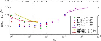
Figure 14 shows the compensated torque
 $Nu_{{\it\omega}}$
as a function of
 $\mathit{Ta}$
for the four values of the vortical wavelength studied. Experimental data by Martinez-Arias et al. (Reference Martinez-Arias, Peixinho, Crumeyrolle and Mutabazi2014) and DNS data by Ostilla-Mónico et al. (Reference Ostilla-Mónico, Huisman, Jannink, van Gils, Verzicco, Grossmann, Sun and Lohse2014a
) is also plotted. It is worth noting that experimental data will have some end-plate effects, even if the aspect ratio
 ${\rm\Gamma}$
of the experiments is larger than 30, while the DNSs have periodic axial boundary conditions. Even so, very similar behaviour can be seen. The transition to the asymptotic scaling laws of the ultimate regime seem to occur around the same value of
 $\mathit{Ta}$
, but are less pronounced the smaller the vortical wavelength is.
Compensated torque
 $Nu_{{\it\omega}}$
versus driving strength
 $\mathit{Ta}$
for
 ${\it\eta}=0.909$
and the three different vortical wavelengths. Experimental data from the
 $T^{3}C$
apparatus (
 ${\rm\Gamma}=46.35$
, number of rolls not determined, cf. Ostilla-Mónico et al.
Reference Ostilla-Mónico, Huisman, Jannink, van Gils, Verzicco, Grossmann, Sun and Lohse2014a
) and from (Martinez-Arias et al.
Reference Martinez-Arias, Peixinho, Crumeyrolle and Mutabazi2014) (denoted MPCM14,
 ${\it\lambda}_{z}=2$
corresponds to 30 rolls and
 ${\it\lambda}_{z}=3$
corresponds to 18 rolls) are also plotted. Axial boundary conditions are different in experiments and DNSs. Experiments have end-plates, while DNSs are axially periodic and thus end effects are absent. Both in experiment and in numerics, different branches associated to different states cross at
 $\mathit{Ta}\approx 2\times 10^{8}$
, shown as a vertical dashed line in the graph. This value of
 $\mathit{Ta}$
corresponds to the transition to the ultimate regime for radius ratio
 ${\it\eta}=0.909$
.

The change in behaviour of the
 $Nu_{{\it\omega}}(\mathit{Ta})$
curves can be associated to the change of behaviour of the wind-sheared regions in the ultimate regime. As seen in Ostilla-Mónico et al. (Reference Ostilla-Mónico, van der Poel, Verzicco, Grossmann and Lohse2014b
), plume ejection is suppressed outside the ultimate regime in regions of the flow, the so-called ‘wind-sheared’ regions due to the sweeping by the large scale rolls. This reduction in plume ejection results in a reduced transport of angular velocity (torque). A similar reduction in the torque caused by a mean flow was also seen when forcing the flow with an axial pressure gradient by Manna & Vacca (Reference Manna and Vacca2009). Vortices with a smaller wavelength have smaller wind-sheared regions and thus result in a larger
 $Nu_{{\it\omega}}$
, if this suppression is taking place. After the transition to the ultimate regime, the suppression ceases, and these regions become active ejectors of plumes, leading to increased transport.
The difference between
 ${\it\lambda}_{z}=2.09$
,
 ${\it\lambda}_{z}=3.0$
and
 ${\it\lambda}_{z}=4.0$
is very small for
 $\mathit{Ta}=10^{9}$
, of the order of 5 %, but for the
 ${\it\lambda}_{z}=1.5$
branch the difference is almost 15 %. Only at
 $\mathit{Ta}=10^{10}$
, when the distinction between wind-sheared and ejection regions is completely blurred away, and the whole inner cylinder can emit plumes (or hairpin vortices),
 $Nu_{{\it\omega}}(\mathit{Ta})$
loses its
 ${\rm\Gamma}$
dependence, within the error bars of the numerics. This sudden transition of wind-sheared regions to ejection regions causes the jump we see in the
 $Nu_{{\it\omega}}(\mathit{Ta})$
curve at around
 $\mathit{Ta}=5\times 10^{9}$
for
 ${\it\eta}=0.909$
.
Note that for the largest drivings axially periodic boundary conditions have been used, with only one vortex pair. This does not prevent the creation of two pairs of vortices with wavelength
 ${\it\lambda}_{z}=1.5$
by a breakup of one pair of vortices of
 ${\it\lambda}_{z}=3.0$
in a domain, which has
 ${\rm\Gamma}=3.0$
. And indeed this is seen to happen for the lower drivings both in DNS and experiment. On the other hand, this axial periodicity affects the stability of one pair of vortices of wavelength
 ${\it\lambda}_{z}=1.5$
in a domain of
 ${\rm\Gamma}=1.5$
. Therefore, vortices with
 ${\it\lambda}_{z}=1.5$
might be an artifact due to the numerical constraintment, and not be stable if a system with large
 ${\rm\Gamma}$
at large
 $\mathit{Ta}$
is considered. States with
 ${\it\lambda}_{z}<2$
are not reported in Martinez-Arias et al. (Reference Martinez-Arias, Peixinho, Crumeyrolle and Mutabazi2014).
Even if we do not expect a quantitative agreement of the present DNS results with those of Brauckmann & Eckhardt (Reference Brauckmann and Eckhardt2013a
) and experimental data by Huisman et al. (Reference Huisman, van der Veen, Sun and Lohse2014), as we simulate a different
 ${\it\eta}$
, the results reported in this section even do not agree qualitatively. Brauckmann & Eckhardt (Reference Brauckmann and Eckhardt2013a
) see a maximum in torque for
 ${\it\lambda}_{z}=1.93$
in the turbulent Taylor vortex regime (
 $\mathit{Ta}\sim 10^{7}$
), while in the present simulations for
 ${\it\eta}=0.909$
at the same
 $\mathit{Ta}$
, this maximum is clearly at
 ${\it\lambda}_{z}=1.5$
, and not near
 ${\it\lambda}_{z}=2.09$
. In the experiments of Martinez-Arias et al. (Reference Martinez-Arias, Peixinho, Crumeyrolle and Mutabazi2014), states with
 ${\it\lambda}_{z}$
smaller than one are not reported, and a direct comparison cannot be made.
We also note that the relationship between larger vortices and larger torque in the ultimate regime is the inverse of what was recently reported by Huisman et al. (Reference Huisman, van der Veen, Sun and Lohse2014). Huisman et al. (Reference Huisman, van der Veen, Sun and Lohse2014) found multiple states, with different
 ${\it\lambda}_{z}$
in highly turbulent TC flow. For different states they found that the torque differs less than 5 %, although they note that this might be due to the fact the torque is only measured on part of the inner cylinder, not on the entire inner cylinder. Furthermore their results are for
 $\mathit{Ro}^{-1}\neq 0$
, for higher
 $\mathit{Ta}$
, and for different
 ${\it\eta}$
, as compared with the current research.
6. Summary and conclusions
Numerical simulations of turbulent TC flow in the range
 $10^{4}<\mathit{Ta}<4.6\times 10^{10}$
were performed to explore the transition of TC flow to the (fully turbulent) ultimate regime. The four dimensions of the parameter space were explored, including the dependence of the transition on the radius ratio
 ${\it\eta}$
, the vortex wavelength
 ${\it\lambda}_{z}$
and Coriolis force
 $\mathit{Ro}^{-1}$
or rotation ratio
 ${\it\mu}$
.
First, the effect of the outer cylinder rotation, in the equations of motion in the frame co-rotating with the outer cylinder, present as a Coriolis force, was analysed for
 ${\it\eta}=0.714$
. Depending on the value of
 $\mathit{Ro}^{-1}$
two regimes were identified, (i) the CWCR and (ii) the SCR, both with their respective subregime. Our findings of that chapter culminate in the phase diagram figure 6, in the
 $(\mathit{Ta},\mathit{Ro}^{-1})$
regime (figure 6
a) and in the
 $(\mathit{Re}_{i},\mathit{Re}_{o})$
regime (figure 6
b,c). The transition to the ultimate regime could be observed for all values of
 $\mathit{Ro}^{-1}$
around
 $\mathit{Ta}\sim 3\times 10^{8}$
. However, for these two regimes a rather different behaviour in the scaling laws
 $\mathit{Nu}_{{\it\omega}}(\mathit{Ta})$
was found before the transition. We also found very different flow structures in the respective ultimate regimes in accordance with the description by Brauckmann & Eckhardt (Reference Brauckmann and Eckhardt2013b
). An explanation why the Coriolis force, proportional to
 $\mathit{Ro}^{-1}$
stabilizes the large-scale structures was illustrated; the large-scale structures were found to not vanish at the transition to the ultimate regime for
 $\mathit{Ro}^{-1}=-0.22\approx \mathit{Ro}_{opt}^{-1}$
, unlike what was seen in Ostilla-Mónico et al. (Reference Ostilla-Mónico, van der Poel, Verzicco, Grossmann and Lohse2014b
) for a resting outer cylinder.
After this, the transition was analysed for various gap widths, namely for
 ${\it\eta}=0.5$
,
 $0.714$
, and
 $0.909$
without Coriolis forces, i.e. for
 $\mathit{Ro}^{-1}=0$
. The transition was found to occur at about the same
 $\mathit{Ta}$
for
 ${\it\eta}=0.714$
and
 $0.909$
. However, the transition was considerably delayed to
 $\mathit{Ta}\approx 10^{10}$
for
 ${\it\eta}=0.5$
, due to the combined effects of stabilizing curvature of the inner cylinder, and the reduced shear as well as smaller fluctuations in the vicinity of the outer cylinder. An analogy between the effect of
 $\mathit{Ro}^{-1}$
in the CWCR regime and the effect of
 ${\it\eta}$
on the large-scale rolls was described: decreasing
 ${\it\eta}$
was found to have the same effect as adding a positive
 $\mathit{Ro}^{-1}$
, corresponding to co-rotating cylinders, while increasing
 ${\it\eta}$
behaved like (weakly) counter-rotating the outer cylinder.
Finally, as the large-scale structures were found to be strongest for
 ${\it\eta}=0.909$
, the effect of varying the vortical wavelength was analysed for this value of
 ${\it\eta}$
. As in Martinez-Arias et al. (Reference Martinez-Arias, Peixinho, Crumeyrolle and Mutabazi2014), different branches of the
 $Nu_{{\it\omega}}(\mathit{Ta})$
curve were found to cross around the transition to the ultimate regime. Before this transition, the influence of the vortical wavelength (and, thus, of the aspect ratio) on
 $Nu_{{\it\omega}}$
was quite noticeable. After the ultimate range transition, this effect decreased drastically. The results of our DNS agree qualitatively with those in the experiments by Martinez-Arias et al. (Reference Martinez-Arias, Peixinho, Crumeyrolle and Mutabazi2014) for
 ${\it\eta}=0.909$
even though the axial boundary conditions are different. However, they are qualitatively different from those reported for
 ${\it\eta}=0.714$
by Brauckmann & Eckhardt (Reference Brauckmann and Eckhardt2013a
) and by Huisman et al. (Reference Huisman, van der Veen, Sun and Lohse2014)
In this work, the vortical wavelength by using periodic boundary conditions was fixed. Some of these states might not be accessible in experiment or might be a product of the periodic boundary conditions. Studying the coexistence of different states for large
 ${\rm\Gamma}$
, as is done in Martinez-Arias et al. (Reference Martinez-Arias, Peixinho, Crumeyrolle and Mutabazi2014) or Huisman et al. (Reference Huisman, van der Veen, Sun and Lohse2014), with DNS requires a large amount of computational resources for high
 $\mathit{Ta}$
. Switches between two and three vortex pairs were seen at lower
 $\mathit{Ta}$
for
 ${\it\eta}=0.909$
(Ostilla-Mónico et al.
Reference Ostilla-Mónico, Huisman, Jannink, van Gils, Verzicco, Grossmann, Sun and Lohse2014a
). Switching between states might also occur at high
 $\mathit{Ta}$
, although they are not captured in the DNS presented in this work. In the future, additional DNS for
 ${\it\eta}=0.909$
with large
 ${\rm\Gamma}$
at high
 $\mathit{Ta}$
should be run to improve the understanding of the switching between different states.
Our ambition also is to further understand why the transition is delayed at
 ${\it\eta}=0.5$
, but also the curvature effects on the
 ${\it\omega}$
-profiles in the boundary layers along the ideas of Grossmann et al. (Reference Grossmann, Lohse and Sun2014). Curvature effects at
 ${\it\eta}=0.714$
and
 ${\it\eta}=0.909$
are too small to be appreciated, and the flow for
 ${\it\eta}=0.5$
is still in the transition to the ‘ultimate’ regime. Thus, higher
 $\mathit{Ta}$
simulations for
 ${\it\eta}=0.5$
will provide further understanding on how curvature makes the boundary layers of TC flow different from those of channel and pipe flow.
Acknowledgements
We would like to thank H. Brauckmann, J. Peixinho, M. Salewski and C. Sun for various stimulating discussions during the years. We would also like to thank the Dutch Supercomputing Consortium SurfSARA for technical support, FOM, COST from the EU and ERC for financial support through an Advanced Grant. We acknowledge that these results come from computational resources at the PRACE resource Curie, based in France at GENCI/CEA.
Appendix. Numerical details
A summary of the numerical results for
 ${\it\eta}=0.714$
which are new to this manuscript. For the other data points see Ostilla-Mónico et al. (Reference Ostilla-Mónico, van der Poel, Verzicco, Grossmann and Lohse2014b
). The first column shows the driving,
 $\mathit{Ta}$
. The second and third column show the outer cylinder rotation as either a Coriolis force
 $\mathit{Ro}^{-1}$
or a rotation frequency ratio
 ${\it\mu}={\it\omega}_{o}/{\it\omega}_{i}$
. The fourth column shows the non-dimensionalized torque,
 $Nu_{{\it\omega}}$
. The fifth column shows the number of grid points used in azimuthal (
 $N_{{\it\theta}}$
), radial (
 $N_{r}$
) and axial direction (
 $N_{z}$
). All of these simulations use a rotational symmetry order six in the azimuthal direction, and are for
 ${\rm\Gamma}=2.09$
.

A summary of the numerical results for the various geometries at
 $\mathit{Ro}^{-1}=0$
, i.e. for resting outer cylinder, which are new to this manuscript. For the other data points see Ostilla-Mónico et al. (Reference Ostilla-Mónico, Stevens, Grossmann, Verzicco and Lohse2013) and Ostilla-Mónico et al. (Reference Ostilla-Mónico, Huisman, Jannink, van Gils, Verzicco, Grossmann, Sun and Lohse2014a
). The first column shows the driving,
 $\mathit{Ta}$
. The second and third column show the radius ratio
 ${\it\eta}$
and the aspect ratio
 ${\rm\Gamma}$
. The fourth column shows the vortical wavelength
 ${\it\lambda}_{z}$
. The fifth column shows the non-dimensionalized torque,
 $Nu_{{\it\omega}}$
. The sixth column shows the amount of grid points used in azimuthal (
 $N_{{\it\theta}}$
), radial (
 $N_{r}$
) and axial direction (
 $N_{z}$
). We note that the
 $\mathit{Ta}=1.11\times 10^{10}$
,
 ${\rm\Gamma}=4$
,
 ${\it\eta}=0.909$
simulation was done using
 $n_{sym}=10$
.