

1 Introduction
This paper explores the link between housing markets and the portfolio allocation of households in a world of changing demographics and shifting pension arrangements. The link between pension reform and the demand for – and price of – housing has not been studied extensively. But housing is the most significant part of wealth for many households; the link between the structure of pension systems and patterns of home ownership is likely to be significant. We investigate optimal decisions over saving, portfolio allocation, and housing tenure in an environment where there are several assets to choose from, options to rent or buy a house, and where there are multiple sources of uncertainty. Several stochastic, calibrated models have studied the impact of uncertainty, both in incomes of individual households (which is largely idiosyncratic) and in the rates of returns on some assets, on life cycle choices.Footnote 1 Beginning with Henderson and Ioannides (Reference Henderson and Ioannides1983), relatively few models allow for the special dual role of housing in the economy; see Berkovec and Fullerton (Reference Berkovec and Fullerton1992), Cocco (Reference Cocco2005), Iacoviello (Reference Iacoviello2005), Lustig and Van Nieuwerburgh (Reference Lustig and Van Nieuwerburgh2005) and Yao and Zhang (Reference Yao and Zhang2005). To our knowledge, there has been no systematic study of the interaction between housing and pension saving decisions at the macroeconomic level.
The main aim of this paper is to analyse the impact of shifting demographics and the changes in pension arrangements in a model that includes housing as both an investment asset and a consumption good. Using the model, we consider the impacts on welfare, on housing conditions and on macroeconomic aggregates of some specific pension reforms.
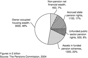
It is very likely that the links between housing, shifting demographics and changes in the structure of state pensions are of great economic significance. Figure 1 shows a snapshot picture of the balance sheet of UK households at the end of 2003. Direct holdings of residential property (owner-occupied housing) made up just under 50% of a comprehensive measure of wealth that includes an estimate of the value of accrued PAYGO (pay-as-you-go) state pensions. Private pension savings make up about 20% of all wealth. Other net financial assets are about 7% of net worth. The value of accrued claims to future government unfunded pensions (both state pensions and promises to public sector workers) make up about 25% of net household wealth. The scale of knock-on effects on portfolio allocation of demographic changes and shifts in pension arrangements is likely to be large. And because houses are hardly traded internationally – unlike claims on financial assets – the scope for induced impacts upon house values and rents is also large.
Balance sheet of UK households at the end of 2003

We embed the decision making of individual households within a model of overlapping generations to derive aggregate demand for various asset classes, allowing for feedbacks from demand changes on to house prices. We calibrate the model so that it broadly reflects features of the UK economy. We then use the model to assess how changing demographics and their interaction with pension reform affect the welfare of different cohorts and generate changes in savings, portfolio allocation, the overall demand for housing, and the choice of housing tenure between ownership and renting. We examine in some detail the welfare effects of different state pension policies.
Using a standard OLG model with several sources of uncertainty, we find that the impact of ageing and of reform of social security upon the demand for housing and the level of owner occupation is substantial. The overall structure of household asset holdings – in particular, the split between real and financial assets – is sensitive to demographics and to the generosity of state run, PAYGO pensions. We find that a significant reduction in the generosity of the state pension is likely to benefit most members of future cohorts – the cost to the current generation of households is not negligible. While this is already true in a model without housing, our new finding is that the size of the welfare effects of pension reform upon different generations is significantly affected by the availability of flexible mortgages.
1.1 Related literature
In the wake of the seminal work of Auerbach and Kotlikoff in the 1980s (see Auerbach and Kotlikoff, Reference Auerbach and Kotlikoff1987), several stochastic, calibrated models based on life cycle optimization in an overlapping generations framework have been developed. There is now a substantial literature that uses calibrated models to address issues of risk allocation in a world with less than perfect risk-sharing opportunities. Much of that literature focuses on the US economy – Hubbard and Judd (1987), Imrohoroglu et al. (Reference Imrohoroglu, Imrohoroglu and Joines1995), Storesletten et al. (Reference Storesletten, Telmer and Yaron1999), Campbell et al. (Reference Campbell, Cocco, Gomes, Maenhout, Campbell and Martin2001) present results from models calibrated to the US economy. De Nardi et al. (Reference De Nardi, Imrohoroglu and Sargent1999) and Kotlikoff et al. (Reference Kotlikoff, Smetters and Walliser1999) look specifically at the transitional and long-run impacts of phasing out unfunded, state pensions in the US. Miles and Černý (Reference Miles and Černý2006) developed a simulation model of the Japanese economy to analyze the macroeconomic and microeconomic implications of ageing. That model allowed for the impact of various sources of uncertainty and assessed how the level of welfare of cohorts might evolve under different assumptions about the reform of social security.
All these models study the impact of uncertainty both in incomes of individual households (which is largely idiosyncratic) and of the rates of returns on some assets, but they do not allow for the special role of housing in the economy. Housing is an important asset in the portfolio of wealth of most developed economies. We calibrate our model to match features of the UK economy. The UK has a level of owner occupation of just under 70% – a level that is about average across developed economies. The total value of owner-occupied housing in the UK economy in 2003 was around three times GDP and greater than the gross value of financial assets held by the household sector. The importance of housing in UK household balance sheets is not unusual – across most economies, the value of residential property is greater than the value of net financial assets. Housing not only comprises a very large proportion of the net worth of households, it is also a unique asset. Housing is a durable good, which yields a substantial flow of real benefits to its owner – the implied value of owner occupation. It can also – and certainly in the UK has fairly consistently over the past 40 years – generate real capital gains. Houses and apartments are also one of the few forms of wealth where the scope to borrow against the asset as collateral is significant. Clearly, the characteristics of residential property are very different from equity investments and from investments in bonds or in cash.
We develop a model designed to allow us to investigate how demographic change and the evolution of social security will impact welfare, portfolio holdings, and housing choices for different generations. The key features of the calibrated model are that it allows for:
1 uncertainty over individual incomes,
2 stochastic rates of return on risky assets and for house prices,
3 a PAYGO pension system with pensions partly linked to incomes and which are also partly flat rate,
4 some scope for households to borrow for house purchase,
5 a rented sector providing an alternative to owner occupation,
6 a bequest motive.
We calibrate the model so that it generates results which broadly match some (but not all) key features of households' decisions on saving, borrowing, and housing choices (renting versus owner occupation and the size of the house or apartment). We then use it to explore the impact of various policy changes upon the welfare of different generations, on portfolio choices, upon the demand for housing, and on the stock of wealth held by households, both within and between generations.
We also assess how changing the role of housing affects the impact of pension reform. In some simulations, we assume home ownership is not possible. Comparing these results to the base case, where we allow home ownership, allows us to assess how much of the impact of pension reform comes about through changes in the demand for owner-occupied housing.
In the next section, we describe the model structure. We then begin our description of the simulation results by focusing on results for existing households at a set of parameters that represents a stylized version of the economy. We look at household and aggregate results. We then look at alternative scenarios for the future where two types of pension reform are considered. These are:
1 Reductions in the generosity of the state pension on a scale to keep the budget-balancing contribution rate constant (which requires a gradual fall in the average replacement rate from around 30% in 2004 to under 20% by 2050)
2 A gradual but persistent rise in the retirement age – or the age at which the PAYGO pension is received.
2 The model
We build an overlapping generations model with time-varying demographics, unfunded pension scheme, and housing and rental markets. The model is calibrated to broadly reflect features of the UK economy. Every year a new generation of households enters the model at age 20. Households face an uncertain life span, and do not survive beyond the age of 90.
Households are endowed with an uncertain and uninsurable stream of income. They earn labour income up to an exogenously given retirement age. Labour income consists of a deterministic component  t, which is augmented by a stochastic element. The impact of stochastic shocks is persistent. In retirement, households rely upon accumulated savings and a state pension, the value of which depends partly on the salary earned at the end of the working life. We will set the tax rate levied upon labour earnings to balance the state pension system and will not allow deficit financing.
In addition to labour income, households may receive bequests. The mechanics of intergenerational transfers is discussed in greater detail below.
2.1 Households' decision problem
Households are assumed to be rational, forward-looking and to solve a stochastic dynamic programming problem. They form expectations about future income, risky asset returns, and house prices, and receive utility from consumption of goods, and from consumption of housing services. We assume that households make choices in each period of their lives about:
(a) how much to spend on consumption (C t),
(b) whether to own a property or to rent (αtH),
(c) what size of property to live in (H t),
(d) how to allocate financial wealth between safe assets (cash, denoted by B t) and risky assets (equity, denoted by S t). where the latter are unpredictable but, on average, have a higher return,
(e) how much to borrow (D t) against ownership of property (which is the only means to acquire debt and then is subject to various limits).
In some simulations, we do not allow investment in housing, or borrowing against it, and only allow renting.
Preferences
The household utility maximization problem is given by the value function

which is maximized with respect to the choice variables spelled out earlier and is subject to a budget constraint detailed in the next subsection. Parameter δ is a constant time discount factor and l t is the probability of surviving period t, thus (1−l t) represents the probability of dying in period t. As T is the last possible period of life (or maximum age to which one can live), l T=0. B(w t+1) is a bequest function – a household receives utility from the knowledge that if they die during period t, their heir receives wealth w t+1. U(C t,H t) is a felicity function defined by

The reciprocal of η is the elasticity of substitution between housing and consumption of goods. This elasticity of substitution is different from the intertemporal elasticity of substitution, γ−1. With this type of preferences, γ also reflects risk aversion. χ is a parameter reflecting the relative value of housing and consumption in the utility function. We will set these parameters so that the simulation results give a broadly plausible pattern of household decisions over the life cycle.
Furthermore, we allow for the preference for consumption to depend on the age of the household – this is reflected by the McClements' equivalence scale m t. The McClements' scaleFootnote 2 allows for the fact that household utility from a given flow of consumption may change with the structure of the family. The McClements' scale follows a hump-shaped profile, reflecting average household size over the life cycle, where children's consumption is given as a fraction of adults' consumption. We calibrate the equivalence scale according to data obtained from the UK Family Resources Survey (2003). For simplicity, we assume that the equivalence scale is exogenous.
To simplify the notation, t=0 corresponds to the age of 20 and T=70 corresponds to the age of 90 when all households still alive die with certainty. Then, with the standard time-separable expected utility model, the value function can be reformulated as

The budget constraint
The value of labour income plus net assets at the start of a period t (including ownership of housing from the previous period) is denoted by x t – this is a comprehensive measure of current net wealth after receipt of labour income. If a household buys a property, it has the option to borrow an amount up to a maximum level, which we allow to depend on the value of the owned house. If the household rents, it pays an amount which is the product of the rental yield r tH and the value of the house. In some simulations, we only allow renting.
Denote the price per unit of housing by p t, then the house value is equal to p tH t. After deciding about the level of consumption C t, the size of the house H t, mortgage D t, and safe investment B t, the amount of risky investment S t is defined by one of two conditions depending on whether the household owns (αtH=1) or rents (αtH=0).


All choice variables must be non-negative (C t,H t,B t,D t⩾0), so the condition S t⩾0 naturally forms the budget constraint.
In the model, a house is an investment asset as well as a durable consumption good that can be enjoyed over multiple periods. Households optimally decide whether to rent or own a house by considering the risk-return profile of the housing asset, opportunity costs (equity returns, safe returns), funding costs (the mortgage interest rate), and costs of alternative housing services (renting). However, for wealthy households, house ownership is generally more attractive than renting for a number of reasons. First of all, although future house prices are uncertain, we calibrate the model so that on average they provide positive returns and are independent from other asset returns, so house ownership is desirable for investors who wish to diversify their portfolios. In addition, house ownership is taxed favourably (in the UK and many other countries) so that capital gains on housing assets can be realized tax-free. Finally, we calibrate the model so that renting costs are higher than net housing funding costs given by the mortgage rates minus expected house price appreciation. This is realistic for the UK. However, renting may be preferable for credit constrained households for whom the downpayment requirement limits the ability to buy a large enough house.
Formally, wealth held by a household consists of two parts: financial wealth w tF and housing wealth w tH

Financial wealth includes both safe assets and risky assets (which we can think of as equity) and is net of debt

 is the stochastic real rate of return on risky assets (which we also call ‘equities’). r t is the safe rate of interest at time t. r tB is the interest rate on mortgage debt. Investment in housing (or housing wealth) is defined as

Housing wealth equals zero only when the household is renting (αtH=0).
The dynamics of net worth is determined by the value of risky and non-risky investments, net of debt, plus the value of housing, current labour income y t, and the amount of bequest received by the household


The availability of credit
The borrowing capacity of a household is based on labour income and the value of collateral (the house or apartment). We assume that debt can be no greater than a fraction (λH) of the value of the house and debt repayments can be no larger than a given fraction (λy) of income. Debt repayments assume that borrowing is in the form of a fixed term repayment (i.e. amortizing) mortgage.Footnote 3 Debt must be repaid by retirement at age T R. Then, the number of remaining years over which debt is to be repaid is denoted by T tM=min (25, T R−t). Thus, the maximum amount the household can borrow is defined as

In setting λH<1, we assume that the fraction of a house financed from saving can be no less than a given percentage.
Bequest motive
We allow for there to be a bequest motive. The assumption made about bequests is an important one in any model of saving and portfolio allocation. The impacts of reform to PAYGO pension systems and the holding of residential property are likely to be sensitive to whether households have a bequest motive.
Bequeathable wealth is defined as the sum of financial and housing wealth −w t. It is always non-negative as the amount of borrowed funds is always collateralized by the value of property. The bequest function is

where the parameters  and
 reflect the strength of the bequest motive. When
 there is no bequest motive, that is B(w t) is independent of w t.
Labour income and state pension
Pre-tax labour income y t is the product of an underlying deterministic trend t and a stochastic component. The deterministic part is a function of age and is calibrated to reflect the average lifetime earnings profile in the UK, peaking at the age of 50 at about twice the salary of a 20-year old (see Miles, Reference Miles1997). The deterministic profile also accounts for productivity growth – productivity is assumed to grow at rate g P. The random component of income reflects idiosyncratic, persistent income shocks u t
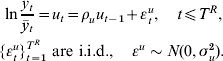
State pension income is a combination of a final salary related component and a flat rate component. The flat rate component is defined as a fixed proportion θ of average retirement salary,  . On average, it makes up two-thirds of the pension; the rest is the salary related component, which is agent specific. For retired households aged t>T R, pension income y t is equal to

where the average replacement rate θ of the pension, also called pension generosity, is set to be around 30%. Every year pension income is adjusted for productivity growth g P. Pension income is assumed to be tax-free.
Equity and safe returns
Equity returns are log-normal i.i.d

We assume these return processes are invariant to domestic saving and portfolio choice. This is in contrast to the assumption about house prices and rental yields, where changes in aggregate demand are allowed to influence the house price process and the rental rate. This seems a natural set of assumptions to make for a model calibrated to a relatively small open economy like the UK. UK households and financial institutions can access global capital markets; but houses are non-traded goods, specific to the UK, and construction is subject to planning restrictions, which limit supply.
House price process and rental yield
We assume that the price of any particular house consists of two components: an overall, aggregate average house price  t and an idiosyncratic (house specific) element. Log house prices p t, relative to the average price, follow a mean reverting process
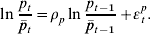
The shocks εtp are independent, normally distributed with mean zero and standard deviation σp. The average house price is set to balance the aggregate demand and supply of housing, as will be explained in Section 2.4.
2.2 Demographics and transfer of wealth among generations
To analyze the impact of various public pension policies we embed the household decision model within an overlapping generations model. All households that are born at time s belong to the same cohort s. These households have common deterministic labour income profile t, but are each subjected to different idiosyncratic income shocks u t, house price shocks εtp, and risky returns t. Households in different cohorts have different average incomes because of productivity growth,Footnote 4 and will face a different lifetime profile of average house prices. Furthermore, in any given year, all living households face a common average house price profile t and rental yield profile r tH.
We assume that wealth held by households at the time of their death is inherited by younger generations. The amount of bequeathable wealth w t is equal to the sum of net financial wealth and the value of owner-occupied house. We assume that bequests are passed on to the generation born T B years later than the parent cohort. To eliminate the need for the amount of received bequests to become another state variable, we simplify the bequest transfers by assuming that bequests are redistributed evenly across the younger cohort. The bequest span T B is set at 30 years.
We denote by N t(s) the number of individuals aged t years at time s. We use UN population data projections up to 2050 to generate values on N t(s), after which we allow the population composition to change according to given mortality rates. The arrival of 20-year-old households is set at such a rate that after 2050 the total population is in a steady state. The mortality rates are obtained from the interim life tables for Great Britain (Office of National Statistics, 2004b).
2.3 Fiscal policy
The model assumes an unfunded pension system that redistributes income from working to the retired households. All workers are taxed at a rate of τ(s), and all proceeds are used to fund pensions of retired households. The pension system is balanced in every period, hence each tax rate τ(s) implies a unique pension generosity θ(s), and vice versa.
Denote the retirement age in period s by T sR. Assuming that productivity (i.e. labour income) in the economy grows at constant rate g P, the income adjusted support ratio S y(s) is defined as
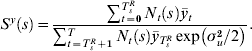
S y(s) at any time s describes the number of retired households whose pension can be covered by the wage bill of one working household in a scheme with a 100% average replacement rate. In other words, the denominator represents the pension bill should every pensioner be given an average last-period-at-work salary adjusted for productivity growth, cf. equation (14).
The pension system is balanced by setting the labour income tax rate τ(s) at the level where tax receipts in a given year exactly match the pension liabilities

where θ(s) is the average replacement rate in period s. This calculation reflects the changing demographic structure, characterized by N t(s). The number of households of each age are based on UK government actuaries projections of the UK population. In the year 2000, the income adjusted support rate is 3.65, which implies the labour income tax required to support the replacement rate of 30% is 8.2%; this rate increases approximately by a factor of 1.6 by 2050 if pensions remain equally generous relative to income.
2.4 Housing and rental market equilibrium
To calculate housing demand in a given year s, we need to compute the optimal demand for housing services of all cohorts alive in that year, i.e. cohorts s, s−1, …, s−T+1. We use a large number of realizations of income shocks and idiosyncratic house price shocks at the household level to calculate individual demands for housing for many households of different ages at each point in time. Let us denote the average housing demand of households of age t in cohort s by  t(s). Then the aggregate housing demand D(s) at time s is formed by summing demand across all households alive in that period
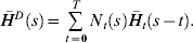
In the overlapping generations model, we calculate the aggregation from year 1990 until 2110. Using the aggregate housing demand, we calculate house demand growth as In D(s)/D(s−1). In a similar way, we calculate aggregate demand for rental housing DR(s) and growth of demand for rental housing In DR(s)/DR(s−1).
In order to obtain equilibrium house prices, we calculate what the aggregate growth in house supply is each period based on an assumed price elasticity of supply of 0.5 – a figure which is the average of all the estimates of the UK housing supply elasticity reported by Barker (Reference Barker2004). For the historical periods (up to 1990), we set the growth rate of average house prices equal to the actual average long-term real house price growth in the UK (since 1945) of about 2% a year. For the simulation period (1990–2110), we set the deterministic growth rate of average real house pricesFootnote 5 each period at a level that matches the change in aggregate demand to the aggregate change in supply, based on the assumed supply elasticity, i.e.
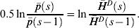
The left-hand side of equation (18) is the change in supply of housing; the right-hand side is the change in demand. This means a 1% increase in the demand for housing requires a 2% increase in average house prices. For the periods after 2110, we approximate the subsequent house price growth by the growth rate observed in 2110.
We assume that there is a less than perfectly elastic supply of rental properties at any house price level. We assume that a 1% increase in the demand for rental housing raises the rental yield by 1/50 of 1%

So a 50% rise in the demand for rental property would, in addition to any impact on house prices from any associated increase in the overall demand for residential property, also have an effect on the relative price of rental to owner-occupied property by raising the rental yield by 1% (from an initial level at the start of the simulation period set to 4%).
Searching for equilibrium house prices and rental yields requires an iterative procedure. In every iteration, we solve the household optimization problems with the deterministic time profile of average house prices and rental yields that would have cleared the market demand in the previous iteration. We iterate to a fixed point where the growths in aggregate demand and in aggregate supply match, assuming a price elasticity of 0.5 in each period. In addition, the aggregate demand for rental housing must match the supply of rental properties, given a yield elasticity of 1/50.
2.5 Model equilibrium
For any pension policy θ(s),T sR, the equilibrium consists of a set of value functions, decision rules, average house prices, and rental yields such that:
1 given pension policy θ(s),T sR, deterministic average house price profile
 (s), deterministic rental yield profile r H(s), and average bequest transfers w tB(s), the households in each cohort maximize their life-cycle utility (1) subject to the constraints,
2 bequests from any one cohort are redistributed to younger cohorts born T B periods earlier,
3 pension system is balanced, i.e. (16) holds in every period s,
4 housing market clears, i.e. (18) holds in every period s,
5 rental market clears, i.e. (19) holds in every period s.
3 Calibration
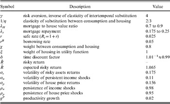
We set the parameters of the model in the following way: first, where a parameter is one about which we have some evidence from micro studies (e.g. on risk aversion or on the volatility and persistence of household labor income shocks), we will use that to guide the choice of parameter; for parameters where micro studies have a less clear message, we will set parameters to generate simulation outcomes for the base case that in recent years match the data for the UK economy. Table 1 summarizes parameter values used.
Parameter values

3.1 Preference parameters
Survey evidence from the US and from Germany suggests that the average coefficient of relative risk aversion is close to 4. Barsky et al. (Reference Barsky, Juster, Kimball and Shapiro1997) undertook a major survey of attitudes to risk among US households; they found great variability of risk aversion among a sample of around 12,000 US citizens. They estimate that the mean degree of risk tolerance implied a coefficient of risk aversion of around 4. A more recent survey of the attitudes to risk of a representative sample of 22,000 German households showed that the average degree of risk aversion is almost exactly equal to that suggested by the large-scale surveys of US households. We use that average value and set the risk aversion parameter, γ, equal to 4.
To tie down the discount rate and the bequest preference parameter, we look to match the UK evidence on the overall saving rate and on the pattern of inheritances. It is the net national savings rate that corresponds to the household saving rate in this model because the government runs a balanced budget and implicit in the model is the assumption that corporations distribute their income – all saving is done by households. The UK net national savings rate in recent years (2000–07) has been slightly above 4.5%. We find that in the base case (where the replacement rate of the state pension is held constant) – and given other parameter estimates – a discount rate of marginally under 1% a year generates a saving rate that averages 4.6% in the 2000–06 period. We set δ to 0.99.
How important bequests are, relative to life cycle smoothing motives, in accounting for overall levels of wealth holdings, is controversial. Even in economies like Japan – where savings rates have been high and family bonds between generations are seen as strong – the bequest motive may not actually be very strong. Recent work of Horioka (Reference Horioka2001) suggests that the bequest motive in Japan may be relatively weak. A survey of motives for saving undertaken by the Central Council for Financial Services (Bank of Japan) showed that under 4% of those surveyed listed bequests as a motive for saving (2003 fiscal year). It is not plausible that in the UK – where the household savings rate has been very much lower – the bequest motive is much higher than in Japan. So there is some justification for assuming that there is a relatively weak bequest motive. (Accidental bequests will, however, naturally arise in a model where annuities markets are less than perfect or where households have an incentive to own their own home while elderly. We find that if we assume that annuities markets are imperfect, unintended bequests are important.)
We set the bequest parameter at a relatively low level. Sefton et al. (Reference Sefton, Dutta and Weale1997) and Weale et al. (Reference Weale, Dutta and Sefton2001) show in a carefully calibrated model that in order to best fit the distribution of actual bequests of UK households, using a life-cycle model of spending and saving, it is necessary to assume a small bequest motive. They find that assuming no bequest motive generates too few bequests, but setting the motive at a high level generates too high a proportion of households leaving significant bequests (relative to their resources). There is also a good deal of survey evidence that many UK households say they aim to leave a bequest to their children. It is highly implausible that all bequests are accidental. In the light of that we set the bequest motive at a moderate level:  . Thus, the utility from a bequest depends on (0.1+w t+1)1−γ. The value of
 is chosen so as not to distort the saving behaviour of young people who have small but non-zero probability of dying and for whom
 would mean they have to set aside bequeathable wealth early in life, contrary to empirical evidence.
We set key housing preference parameters (which are the elasticity of substitution between consumption and housing and the relative weight of consumption and housing in the utility function) so as to generate a level of owner occupation and of the scale of housing wealth in overall household portfolios to match the UK evidence. The overall owner occupation rate in the UK has been very steady at around 68% for the period 2000–06. Owner occupation is relatively low amongst people in their 20s and starts to rise strongly amongst people in their 30s. Owner occupation is much higher amongst those in the second half of their working lives. The average age at which people became homeowners in 2003 was around 32.
By the end of 2004, UK housing wealth as a proportion of net worth for the household sector, excluding the value of accrued claims to unfunded state pensions, was slightly below 60%. (Net assets here are all financial assets held by households plus the value of tangible assets net of financial liabilities.) Housing wealth as a proportion of all net assets – including the value of claims upon future state pensions – was just under 50%. Housing wealth as a proportion of all wealth for UK households typically peaks in the early 30s (which is when many households have recently become homeowners and moved out of the rented sector, but have yet to accumulate substantial savings).
We set the elasticity of substitution between consumption and housing,1/η, equal to two-thirds and the weight of housing in the utility function to 0.8. With these parameters in the base case simulation, we find that housing is just over 50% of all wealth in the 2000–06 period and the owner occupation rate is around 70%. With these preference parameters – and given the other parameters of the model – we find that the typical age at which households would buy their first home is in their early 30s.
3.2 Asset prices
We take the mean return on risky assets (‘equities’) to be 6.5% and annual volatility to be 17.5%. This matches the historic record on equity prices across developed countries over the past 100 years (see Dimson et al., Reference Dimson, Marsh and Staunton2002).
House prices in the UK have been relatively volatile.Footnote 6 Over the longer term in the UK house prices have risen by about 2% a year in real terms. Shocks to house prices seem persistent, but not all shocks are permanent. (In other words, prices do not seem to follow a random walk around a trend. Rather they may swing above and perhaps below trend for sustained periods.) Our specification of the process for house prices allows for this feature. We set the persistence parameter at 0.95, which generates relatively long duration swings in prices. The annual volatility of shocks we set to just over 15.5% – a level that makes house price volatility comparable to the volatility of equities, which UK evidence suggests is appropriate.
Average rental yields in the private rental market for residential property in the UK have been at around 5% in recent years. Rent on public sector housing is lower. An overall rental yield of about 4% is plausible; that is where we set it.
We set r (the safe real rate of interest) at 2.5% and the mortgage rate r B at 5%. Using a safe real rate of interest of 2.5% means that we have used a figure a little lower than the long-run average real yield on UK government bonds (gilts). That average yield on longer dated gilts over consumer price inflation has been about 3%, but lower recently. In recent years interest rates on mortgages in the UK have been, on average, approximately 1 to 1.5% above the level of short-term money market rates.Footnote 7 Rates on deposits are below money market rates; the spread between deposit and mortgage rates is likely to be about 2.5%.
In recent years, the typical loan to value ratio of first time buyers in the UK is between 85% and 95%. A down payment of somewhere between 10% and 15% of the property value has been common. At times in the past, this down-payment requirement has been higher. We set the borrowing limits (down-payment requirement) to reflect these facts. We set λ, the maximum loan to value ratio, at 0.9 in recent years, but allow for it to have been lower (at 0.7) before the 1980s and to have gradually risen through the 1980s – the period of mortgage market liberalization in the UK.Footnote 8
We assume that since 1991 households can spend up to 25% of annual labour income on mortgage repayment (λy=0.25); before 1980 we set that ratio lower, at 17.5%, to reflect the rise in the availability of credit which occurred in the 1980s due to mortgage market liberalization.
3.3 Labour income process
We set the persistence of labour income shocks, ρu, and the volatility of shocks, σu, to levels that match the pattern of labour incomes in the UK. We set persistence at a high level (ρu=0.98) to reflect the fact that most shocks have a long-lasting impact on earnings.Footnote 9
The growth of annual labour productivity is set to 2% – which is very close to the UK average over past 40 years.
4 Simulation results
We first describe the base case simulations. We then assess the impact of two pension policy changes: the first involves a gradual reduction in the average replacement rate of the state pension; the second involves raising the age at which the state pension is paid. In the first policy experiment, we assume that the level of the state pension is gradually reduced so that the contribution rate needed to balance the state pension system is constant at 8.2%. In this scenario, the average replacement rate of the state pension falls from 30% to about 19% by 2050. In the other policy simulation, we allow for a continuing rise in the retirement age, which helps to reduce the tax burden, but we assume a constant pension generosity (replacement rate of 30% on average). We then describe results of the impact of pension reform upon the welfare of different generations when we rule out any impact on the demand for owner-occupied housing.
4.1 Scenario A: Base case
In the base case, we assume that the average replacement rate of the PAYGO pension remains constant at 30% for every cohort. (The replacement rate is not the same for those within a cohort because there is a flat rate element to the pension, which generates some redistribution within the system.)
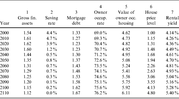
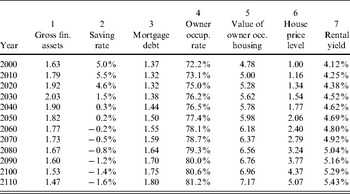
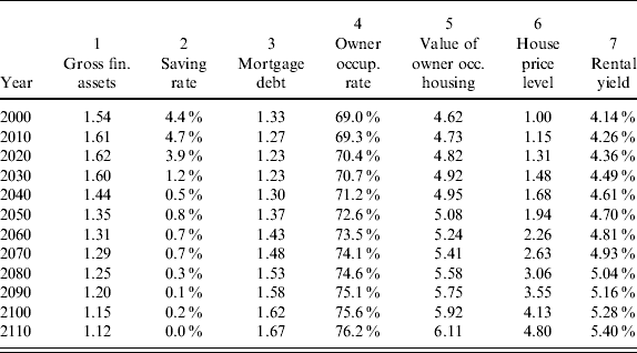
Table 2 summarizes how the aggregate outcomes evolve over time in the base case. In forming the aggregates and tracing their development over time, we sum over the decisions of members of every cohort, using demographic projections to determine the relative numbers of people from each cohort alive at each date. While we focus on the average decisions of the members of that cohort, within any cohort there is considerable heterogeneity because idiosyncratic income shocks play a major role in the model. Given the way that we picked the parameters, it is not surprising that we do a good job in matching the key features of the macroeconomy at the start of the simulation period, so outcomes for 2000 are a good match against the recent UK data (in terms of owner occupation, the saving rate, the value of owner-occupied housing relative to aggregate incomes, the stock of debt, and the yield on rental property).
Aggregate results, scenario A
(Columns 1, 3, and 5 show values relative to average pre-tax labour income.)
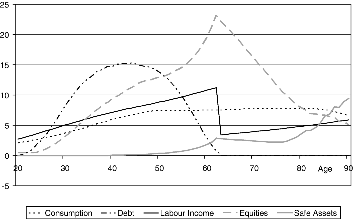
It is also important to generate a plausible pattern of typical life cycle behaviour. We assess that by focusing on the behavior of a particular cohort (that born in 1960). Figures 2 and 3 focus on the average of decisions made by all those households of the 1960 cohort that are still alive at each age. (The great majority of the cohort born in 1960 survive into their 60s and 70s. By assumption, no one lives beyond the age of 90.)
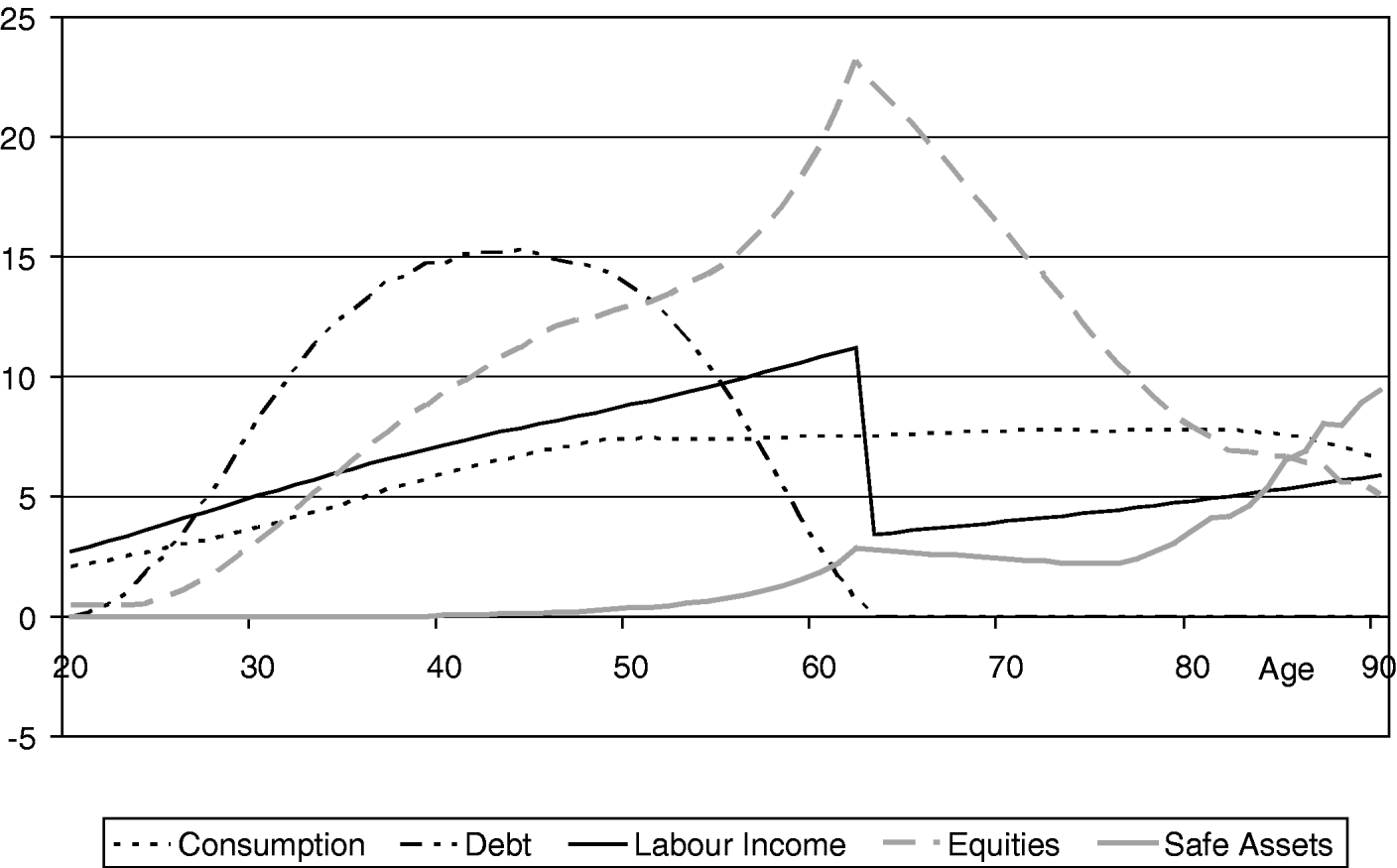
Life cycle portfolios, cohort born in 1960, scenario A
This chart shows five important characteristics of life-cycle decision making – consumption of goods, labour income, amount of borrowed funds and holding of safe assets and equities. These profiles present average (or expected) values obtained by simulating optimal lifetime decisions of 100,000 households. Each household is born at age 20 and starts with no wealth. We assume that if any household is still alive at age 90, it dies then with certainty. Households receive random persistence income shocks, house price shocks, and equity return shocks, which are idiosyncratic across all households.
Owner occupation rate, cohort born in 1960, scenario A
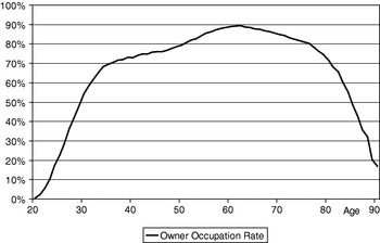
This plot illustrates the average lifetime owner occupation rate of households born in 1960.

Figure 2 summarizes a lot of information about typical behaviour over the life cycle. It shows that, on average, households start to build up debt in the first part of their adult lives. Debt for households typically peaks in the early 40s – by which time a large majority of households are owner-occupiers (Figure 3). Households gradually repay debt over the second half of their working lives, when they also accelerate the rate at which they accumulate savings – most of which are in the form of equities. We should view the portfolio of asset accumulated in this model as corresponding to all assets held directly and indirectly by households. The high equity weights generated by this simulation in the portfolios of financial assets looks unrealistic when compared with the portfolios of directly held financial wealth by UK households. But pension wealth – most of it held indirectly within pension schemes and life insurance companies – is a major part of UK overall household wealth and historically the largest part of that wealth has been in the form of equities.
Note that the profiles of wealth accumulation, debt dynamics, and housing tenure shown in Figures 2 and 3 are the average profiles across the households of a specific generation. Individual profiles are far more jumpy, both because some of the decisions in the model are discrete (e.g. on whether to own or rent a property) and because decisions are sensitive to individual idiosyncratic shocks to incomes and housing wealth, which make individual profiles far more variable than the cohort average.
This is particularly relevant to the interpretation of debt dynamics and housing tenure. All households begin their adult life (at age 20) by renting. The down payment constraint for buying a house is substantial and so few households buy a house until they reach their 30s. However, owner occupation is attractive for households – with real house prices rising on average by about 2% a year and the cost of mortgage debt at 5%, the expected effective user cost of housing for an owner-occupier borrowing the maximum is around 3%. The rental cost is higher and rises from a level of 4% in 2000 and towards 4.5% by 2030. Younger households aim to move into owner occupation fairly early in their life cycle and the great majority remain in owner occupation until well into retirement. Because the typical household can expect to stay in owner occupation for many years, owning a home gives a form of insurance against unexpected house price shocks. Since these shocks are large, there is an element of a precautionary demand for housing. As a result, owner occupation is very high within a cohort once the age of its members is above 40; Figure 3 shows that owner occupation is close to 80% at age 50 and peaks at just under 90% at retirement. Owner occupation rates fall slightly as households move through their 60s and their 70s. Owner occupation amongst those households in their 80s – and for whom the desired stock of net worth begins to fall significantly – starts to drop rapidly. Initially, almost all households borrow as much as they can to finance house purchase. However, during their 40s, there emerges considerable heterogeneity within the cohort, with many households borrowing substantially less than the maximum. All this matches the key features of household choices in the UK.
Once households retire, there is a significant change in the portfolio of assets. The existence of a bequest motive means that, while many households wish to continue holding substantial net assets, the composition of portfolios changes. Increasingly households reduce the proportion of their overall wealth in the form of owner-occupied housing and increase the proportion of wealth in the form of financial assets. As households go past retirement, the composition of their financial assets changes rapidly as people increase sharply the percentage of their assets in safe debt and holdings of risky assets fall sharply. In contrast, very few households in their 30s and 40s hold significant amounts of wealth in safe financial assets. When human capital is still the dominant form of lifetime assets, and when holdings of debt (which has a cost in excess of the return on safe assets) tend to be large, holding safe assets is not attractive; where financial assets are held they are, therefore, overwhelmingly in the form of risky assets. This is a reflection of the assumption that shocks to human capital are largely idiosyncratic and independent of the return on risky assets (which for convenience we call ‘equities’, though which should be interpreted more widely). As we shall see, the pace with which the switch from risky to safe financial assets happens is dependent upon the generosity of state pensions. Overall, households move into owner occupation early in the life cycle and only sell the house and move back to rented accommodation if they are still alive in their 80s. The high average real rate of return on property, relatively high cost of renting and the existence of a bequest motive combine to make housing an attractive asset and one which people are content to dominate their portfolios of wealth for much of their lives.
Aggregate national savings rate
The national savings rate has been calculated as


If PAYGO pensions remain at the same level (relative to average incomes), it is predicted that the level of owner occupation is fairly steady until about 2040 and then rises gently. Owner occupation starts out at just under 70% in 2000 (close to the actual level of UK owner occupation). By 2050, the rate of owner occupation is 73%. By 2075, it is 74%. House prices rise fairly steadily in real terms and the value of houses bought – relative to incomes – also rises gradually. Real house prices double between 2000 and 2052. Financial assets as a proportion of the gross wealth of the household sector steadily rises – and housing wealth falls as a proportion of gross wealth – as the population ages.
The savings rate in the economy starts at about 4.5% in 2000, see Figure 4. The savings rate starts to decline gradually from about 2010, when it stands at close to 5%. By 2031, it is only just over 1% and only 0.8% by 2050. This change is largely driven by demographics: by 2050, there are a substantially higher proportion of retired households who have, on average, a lower savings rate than working households.
4.2 Alternative scenarios – the impact of pension reforms
Scenario B: Constant contribution rate
In this scenario, the value of the PAYGO pension declines gradually relative to average earnings. By 2050, the average replacement rate for newly retired households is down to 19%; in the base case, that ratio stays at 30%. The impact on cohorts born later than 1960 is substantial. For example, the cohort born in 1990, who start work in 2010, react to significantly lower state pensions by accumulating much more wealth by retirement. On average, the value of net worth of this cohort when it reaches retirement (at around 2050) is about 30% higher as a result of lower state pensions. Owner occupation is also markedly higher for this cohort than when state pensions are kept steady relative to incomes. Demand for financial assets is also greater. The proportionate impact of lower state pensions upon the value of residential property and financial assets held is similar, though demand for financial assets does grow by somewhat more.
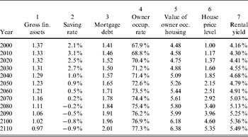
As a result, the macroeconomic aggregates in an environment of falling PAYGO pensions diverge quite markedly from those where the pension replacement rate is held constant. (Table 3 summarizes the aggregate outcomes and how they evolve.) With falling pensions, the owner occupation rate is higher, as is the overall demand for housing; this drives house prices up somewhat faster than in the base case. (The owner occupation and saving rates are actually higher even at the start of the simulation period. This is because we assume in each scenario that agents anticipate the pension policy that is coming. The exact timing of when demand for housing and for financial assets rises under a scenario with falling replacement rates for state pensions will depend on when it becomes clear how policy is evolving.)
Aggregate results, scenario B
(Columns 1, 3, and 5 show values relative to average pre-tax labour income.)

Households are more willing to retain large net holdings of property into retirement. As a result, the overall demand for housing is somewhat higher when the value of PAYGO pensions falls – house prices are about 8.5% higher by 2050. The relatively small impact on house prices but larger impact upon the value of owner-occupied residential property reflects the fact that a switch from renting to buying (relative to the base case) itself is neutral for the overall demand for housing. What is happening here is that with lower state pensions, after tax incomes are higher because the tax rate is lower. Households react to higher post tax incomes and lower state pensions by accumulating more wealth. A high proportion of that extra demand for wealth is a higher demand for housing wealth. This is why house prices and owner occupation rates are markedly higher than in the base case.
Net worth of the household sector relative to aggregate labour income is substantially higher, and rising, when the value of PAYGO pensions (relative to incomes) is set on a declining path, see Figure 4. The overall saving rate is higher for many years – in 2010, it is 5.5% compared to 4.7% in the base case. However, after 2035, the saving rate is lower and it becomes slightly negative after 2055. It may seem counterintuitive that the savings rate is eventually higher in the base case, with relatively generous state pensions than in the scenario where households need to accumulate more wealth to compensate for falling state pensions. This finding is less surprising if one realizes that in the lower state pensions scenario, households keep much more wealth in the form of housing; and capital gains on housing, which are significant, are not part of the income that enters the expression for the savings rate. Net worth of households is always higher when state pension are worth less.
Scenario C: Replacement rate at 30% but increasing retirement age
In this simulation, we allow for a gradual increase in the retirement age from 62 in 2015 to 70 in 2050 – otherwise the environment is as in the base case. Table 4 summarizes the aggregate outcomes for this simulation. When the retirement age begins to rise, the demand for assets held into retirement falls since that wealth sustains consumption over a shorter period. Therefore, as shown in Figure 4, the saving rate is significantly lower – it is only 3% in 2010, 2.7% in 2030, and just under 1% in 2050. The demand for housing rises rapidly. Higher demand for housing is driven by the larger lifetime flow of labour income that is a by-product of later retirement. House prices now double by 2044. Demand for financial assets, not surprisingly, peaks later in life when retirement is pushed back. Although the saving rate out of income is lower when retirement is significantly later, the overall accumulation of wealth (net worth) by cohorts who work longer is higher. The fall in the rate of saving out of income is more than offset by the impact of higher lifetime labour income. The impact on demand for housing and house prices is substantial. This reflects higher lifetime incomes because working lives are longer. Note that households can borrow more if labour income is larger and pension income is lower, because households can only service debt out of labour income and not from pensions.
Aggregate results, scenario C
(Columns 1, 3, and 5 show values relative to average pre-tax labour income.)

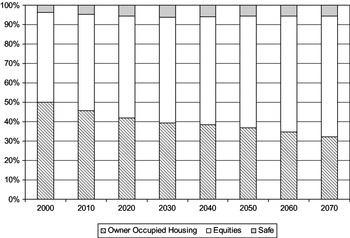
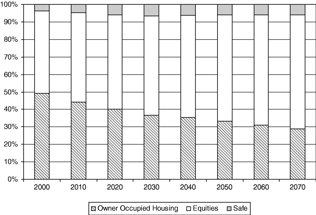
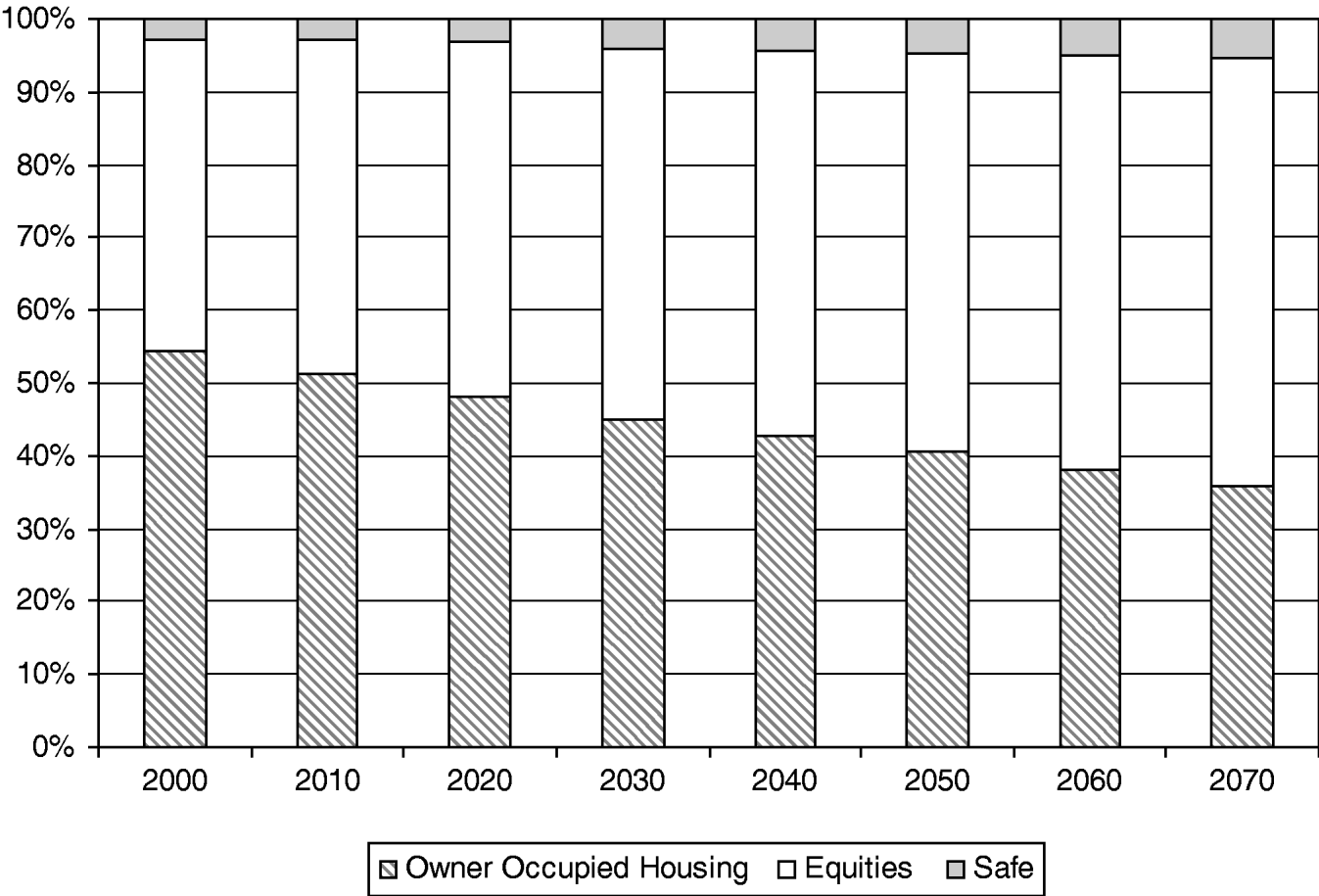
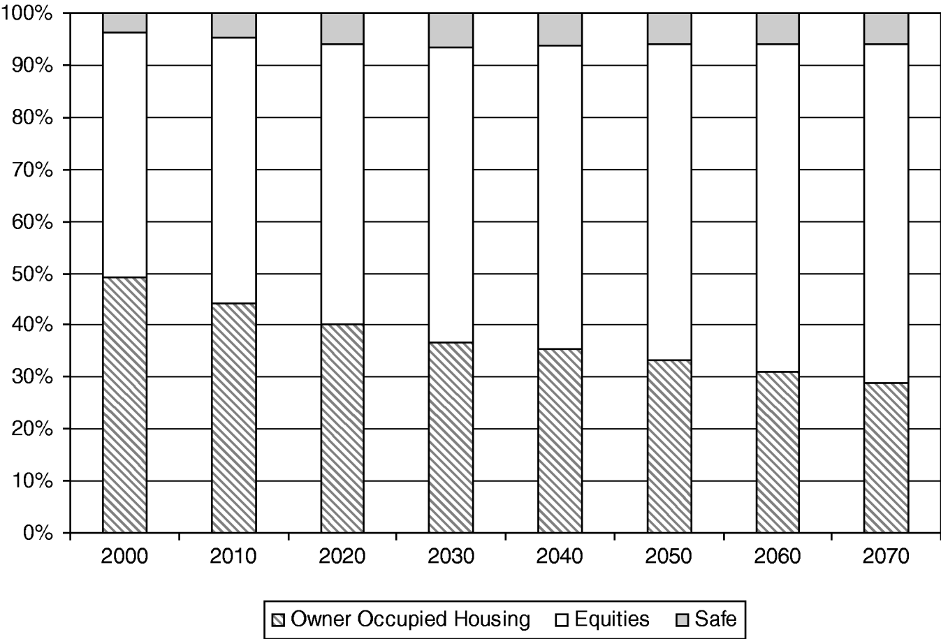
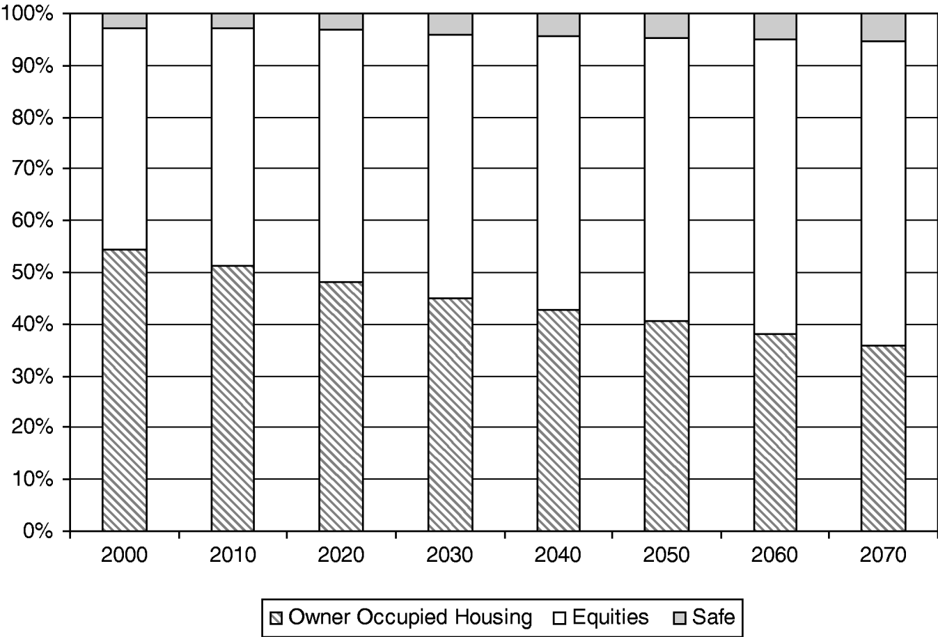
In all scenarios, aggregate gross financial assets rise relative to the value of owner-occupied housing over time, see Figures 5–7. This is because as households age and pay off their mortgage, they accumulate financial assets and, if they live into their 80s and beyond, eventually tend to move out of owner occupation. In contrast, younger households – particularly those in their 30s – hold the great majority of their wealth in the form of newly acquired homes and have relatively few financial assets. Over time, the proportion of households in the later stages of their lives, when financial assets rise in importance relative to housing, increases. But the scale of this aggregate portfolio shift varies depending on the state pension system. When state pensions become less generous, the switch towards financial assets in household portfolios over time is more marked. By 2050, financial assets comprise about 67% of gross assets in the economy relative to the base case (constant generosity of state pensions) of around 62%. However, when the age at which households receive the state pension is significantly later, the switch towards financial assets in gross wealth is slower than in the base case.
4.3 Welfare analysis
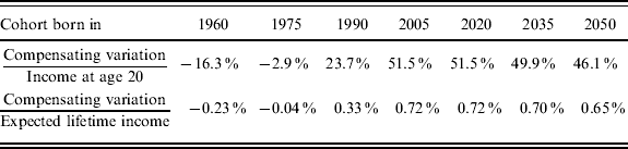
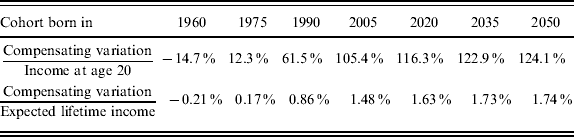
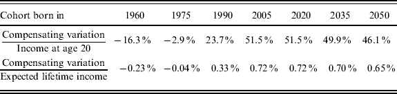
Table 5 shows that, while in the long run a move towards less generous PAYGO state pensions does increase average welfare for future generations, households who are middle aged (the cohorts born around 1960) tend to lose as the value of the state pension is scaled back. We are not able to find a Pareto improving change in the structure of state pensions. In a model where the average rate of return on assets is greater than the rate of growth of the economy, it is not surprising that the long-run impact of reducing the generosity of unfunded pensions is to raise average welfare; it is also not surprising that on a transition there are likely to be losers (see Breyer, Reference Breyer1989). The scale of the gains of the future winner generations from less generous unfunded pensions is, however, significantly greater than the small welfare losses of the current middle aged. The welfare gain for a cohort born in 1990 of lower state pensions, relative to the base case of unchanged pension replacement rates, is the equivalent of just under 25% of initial annual average salary, or about 0.33% of lifetime income. Gains to future generations are higher again. The loss of this reform for the cohort born 30 years earlier (the 1960 cohort) is just above 16% of their average initial income, and only about 0.2% of lifetime income.
Compensating variation of moving from scenario A to scenario B for cohorts born at different dates. The expected lifetime income represents the expected present discounted value of lifetime labour income (discount factor equal to the safe deposit rate of 1.2% p.a.)
4.4 No owner-occupied housing
We assess how much of the impact, particularly on welfare, of pension reform comes about through the knock on effect of reform upon the demand for, and price of, owner-occupied housing. We do this by running simulations where we do not allow for shifts in saving and wealth accumulation to come in the form of greater demand for owner-occupied housing. In this simulation, households just rent their homes.
Table 6 shows the impact on the welfare of different cohorts from reducing the generosity of the state pension when households all rent. The gain to future generations from cutting taxes by reducing the generosity of state pensions is greater when we do not allow for owner-occupied housing. The gain to future generations from having lower state, PAYGO pensions is more than twice as great as when we have owner-occupied housing. This is a substantial difference and one that cannot be accounted for by the small relative differences in house prices and rental yields we observe across the two pension scenarios.
Compensating variation of moving from scenario A to scenario B for cohorts born at different dates. Owner occupation is switched off – only renting is possible. The expected lifetime income represents the expected present discounted value of lifetime labour income (discount factor equal to the safe deposit rate of 2.5% p.a.)
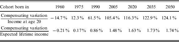
The key insight is that availability of mortgage debt can help alleviate the credit constraint of young households. This is not entirely obvious because, on the face of it, mortgage debt can only be used to finance house purchases. However, young households have an increasing income profile and a long lead time to retirement which means they can, at least before they reach 40, remortgage at a higher level year after year. Effectively, they can add the interest on the mortgage to the principal and use the money that otherwise would have to be spent on mortgage repayments to finance consumption instead. In practice, many mortgages have transaction costs that prevent such topping up, but there are also flexible products, such as offset mortgages, that do permit increased borrowing up to a certain limit. The mortgages in our model resemble the latter type.
Once we understand that flexible mortgages are the channel through which young households can access credit to finance effectively their consumption of goods, the rest of the story is a textbook case of optimal consumption under credit constraints. In scenario A, the pension generosity is high and so is the tax burden on young households. The credit restrictions bind tightly in this case and the availability of extra credit via flexible mortgages is highly valuable. When we remove owner occupation, and with it the availability of mortgages, young households in scenario A suffer more than those in scenario B because of the higher tax burden in scenario A. As a result, the welfare gain of moving from high tax burden scenario A to less generous pensions in B is substantially higher in a model with no owner occupation.
Aggregate portfolios, scenario A

Aggregate portfolios, scenario B
Aggregate portfolios, scenario C
5 Conclusions
The aim of this paper has been to explore the role of housing in a model of life cycle choices for UK households that face various forms of uncertainty, receive PAYGO pensions of various levels of generosity, and have a limited bequest motive. Households also face borrowing constraints. We developed a model calibrated to reflect key features of the UK economy. We derived results on the behavior of cohorts over their life cycle and on the evolution of macroeconomic aggregates in an environment of rapidly changing demographics. We solved the model under various assumptions about how pensions and contribution rates will evolve.
We find that the demand for owner-occupied housing is sensitive to demographic change and to reform of the PAYGO pension system. If PAYGO pension replacement rates remain high as the population ages, the level of owner occupation may rise only marginally over time. Nevertheless, if pension generosity is scaled back sharply, the rate of owner occupation and directly held housing wealth may rise significantly faster. When the pension age is raised significantly, the demand for housing rises most strongly and the demand for financial assets grows relatively less strongly. As a result, there is a marked change in the aggregate pattern of household wealth relative to other pension scenarios. However, one thing all our scenarios have in common is that the importance of owner-occupied property in overall portfolios declines over time. This is despite the fact that owner occupation rates continue to rise, as do real house prices.
The links between the property market, demographic change, and pension reform seem to be significant. One policy conclusion from this paper is that the gain from scaling back the generosity of state pensions are significant; but while the cost of doing so is relatively low for cohorts alive today, it is not negligible. This is not a new result. The new finding is that the size of the welfare effects of pension reform upon different generations is significantly affected by the availability of mortgages. When we do not allow for owner occupation, credit restrictions are higher and so the benefit of easing those restrictions by reducing the generosity of state pensions is larger. This suggests that modelling the interaction between pension reform and the availability of flexible mortgages is important.