Introduction

The past decade has witnessed some of the most detailed studies ever carried out on the mass trends of the terrestrial cryosphere. This is partly due to an increased awareness of ice-sheet processes that can respond rapidly to external forcing, but primarily due to the growth in observational datasets that can (partially) address this problem. There are three main approaches to determining the time-evolving mass balance of an ice sheet, each with its own merits and limitations.

1. 1. The first is the geodetic approach, exemplified by satellite radar and laser altimetry. The measured elevation rate transposes into a mass rate via a mean density field, which is generally inferred from numerical models and/or assumptions about the process responsible for the height change. The elevation changes are normally corrected for variations in firn compaction rate using a firn compaction model (Reference Arthern and WinghamArthern and Wingham, 1998; Reference ZwallyZwally and others, 2005), which requires input fields such as accumulation rates and surface temperature.

2. 2. The second approach is variously termed the mass-budget, flux-divergence or input/output method. Here, mass balance is determined at the drainage basin scale by differencing the influx – the surface mass balance (SMB) for the basin estimated using a regional climate model – and the outflux, determined at the grounding line from observations of velocity and estimates of ice thickness (Reference RignotRignot and others, 2008; Reference Mouginot, Rignot and ScheuchlMouginot and others, 2014).

3. 3. The third approach is to weigh changes in the ice sheet using gravity anomalies derived from the Gravity Recovery and Climate Experiment (GRACE) satellites. Mass change due to glacio-isostatic adjustment (GIA), which is a dominant signal in Antarctica (Reference Sasgen, Martinec and FlemingSasgen and others, 2007; Reference RivaRiva and others, 2009), is subtracted from the recorded gravity anomalies to obtain a mass-balance estimate.

These three methods suffer from both common and different limitations. Altimetry (method 1) has poor coverage at the poles and the Antarctic Peninsula, the mass-budget method (method 2) cannot estimate outflux for grounding lines where ice thickness is unknown (Reference Rignot, Jacobs, Mouginot and ScheuchlRignot and others, 2013) and GRACE (method 3) has an effective resolution of ~300 km. Moreover, and more importantly, results from all the above methods are influenced by errors that are primarily dominated by uncertainties in models which provide estimates for SMB (methods 1 and 2), firn densification (method 1) and GIA (method 3). It is difficult to accurately characterize the uncertainties from these deterministic models, some of which may contain systematic biases which would go unnoticed in each of these approaches (Reference Horwath and DietrichHorwath and Dietrich, 2009; Reference Van WessemVan Wessem and others, 2014). For example, a recently updated version (V2.3) of the Regional Atmospheric Climate Model (RACMO; Reference Lenaerts, Van den Broeke, Van de Berg, Van Meijgaard and MunnekeLenaerts and others, 2012), that has been used in most of the mass-budget (method 2) studies, has a mean SMB that is 111 Gt a⁻¹ higher than its predecessor, with most of the difference (101 Gt a⁻¹) occurring in East Antarctica. Such a systematic bias feeds directly into estimates of mass trends but is extremely difficult to characterize in terms of uncertainties, which thus appear to be significantly underestimated (Reference ShepherdShepherd and others, 2012). Consequently, results from many of these techniques differ considerably from each other (Reference HannaHanna and others, 2013).

As explained above, due to extensive model use and simplifying assumptions, meta-analysis, such as a non-weighted arithmetic average of different results (e.g. Reference ShepherdShepherd and others, 2012), will likely result in a systematic bias and an inaccurate assessment of uncertainty. The latter is true particularly for methods which make use of the same, or similar, geophysical models and yet are assumed to provide independent error estimates. For example, the GIA models IJ05_R2 (Reference IvinsIvins and others, 2013) and W12a (Reference Whitehouse, Bentley, Milne, King and ThomasWhitehouse and others, 2012) may not be considered independent since they use the same geochronological constraint and GPS data. Alternative approaches which reduce the dependence on numerical models have been developed (Reference RivaRiva and others, 2009; Reference GunterGunter and others, 2014), which, following a philosophy similar to that here, attempt to exploit the benefits of some observations to counter the limitations of others (especially in coverage). However, in order to simplify the problem, these methods tend to assume that mass losses due to SMB anomalies or changes in ice dynamics are mutually exclusive, which is clearly an unphysical constraint. Further, firn densification is either ignored or catered for using a firn densification model. The latter generally requires, as a minimum, time-evolving accumulation rates and surface temperature. These are relatively well constrained for the recent past (since ~1979), but prior to that are poorly known, whereas the process takes place over a vertical column that extends back in time over centuries, rather than decades. Changes in climate that affect firn densification prior to 1979 are, therefore, largely unknown and unaccounted for.

Here we present a new approach to mass-balance estimation which, to date, relies the least on geophysical model output. The method hinges on using geophysical understanding incorporated in the model outputs, and auxiliary datasets, to inform prior judgment on the processes of interest: in this case as applied to the Antarctic ice sheet (AIS). For example, we can take advantage of the fact that GIA is a low-power, long-wavelength, temporally invariant signal, and that changes in ice dynamics are temporally low-frequency compared to SMB anomalies, to obtain a decomposition of the observed signal (Reference Zammit-Mangion, Rougier, Bamber and SchoenZammit-Mangion and others, 2014). The classic concept of signal filtering is a starting point for the approach, but recent advances in statistical and computational methods allow us to incorporate uncertainty on the filtered quantities using probabilistic smoothing. The power of the approach lies in its ability to eliminate the need for numerical models to solve for unobserved/unresolved processes, while rigorously handling confounded errors where changes due to, say, ice dynamics and SMB anomalies may be present simultaneously. An added benefit is that since the results provided do not directly employ numerical model output, they can be used to validate the models. An example of this is shown in the Results section.

Theoretical Rationale

When assessing the mass balance of the AIS, we are faced with the task of determining to what extent each process is causing the observed change. Determining the combination of underlying signals is akin to the classic problem in signal processing of source separation: the process of disentangling a mixed signal into its constituent components (Reference Comon and JuttenComon and Jutten, 2010). For illustration, consider the simple case of two components, x ₁ and x ₂, and one set of noisy measurements, y , on the sum of x ₁ and x ₂, represented as

(1)

where I is the identity matrix and e is the observation error. Since we have more components than observations, this problem is said to be under-determined, i.e. if this were a deterministic problem with zero error, e , there would be no unique solution for { x ₁, x ₂}. In statistical terms, if we treat x ₁ and x ₂ as random quantities, this system is said to exhibit prior sensitivity: the judgments placed on x ₁ play a crucial role in the estimate of x ₂, and vice versa. The application of prior, or initial, information leads to the consideration of a bias/variance trade-off – the more informative the prior on, say, x ₂, the greater the risk that inferences on x ₁ are biased.

The challenge, therefore, is to express prior beliefs on x ₁ and x ₂ which are somewhat informative (to aid source separation) but not too restrictive. One such belief, which we will take considerable advantage of in this work, is that of smoothness, or characteristic wavelength (in time or space) of x ₁ and x ₂. Formally, suppose that x ₁, x ₂ and e are Gaussian (i.e. are fully defined by some expectation and variance). Further, assume, for simplicity, that all the initial expectations are zero, and x ₁, x ₂ and e are mutually independent. Smoothness constraints can be imposed on x ₁ and x ₂ by appropriately configuring the covariance matrices, Var(x ₁)= Σ ₁, Var(x₂) Σ ₂. For a field x , if the covariance matrix, Σ , is diagonally dominant, then x is said to be rough (as different components of x are uncorrelated), conversely it is smooth.

It is instructive to consider an extreme case. Assume Var( e ) is relatively small, Σ ₁ ≈ σ² 11 ^T (fully correlated), and Σ ₂ ≈ σ² I (diagonally dominant). Inferences on x ₁ and x ₂ using noisy data, y , can be found analytically via Bayesian updating (e.g. appendix A of Reference Rasmussen and WilliamsRasmussen and Williams, 2006). In this extreme case it can be shown that the expectation of x ₁ will update to the sample mean of y (a low-frequency signal), while the expectation of x ₂ will update to the difference between y and its sample mean (a high-frequency signal). Hence, by simply configuring Σ ₁ and Σ ₂ we are able to separate the signals when x ₁ and x ₂ have different spectral characteristics. Note that this is distinct to the classical application of low-/high-pass filters, since the Bayesian update provides a covariance matrix which incorporates both the marginal (individual) and joint uncertainty on { x ₁, x ₂}.

This approach to source separation is very different to the case when restrictive estimates (e.g. numerical model output for SMB anomalies or a GIA solution) are used for one of the fields. In such a case we would be employing an estimator, , of x ₁ with uncertainty ξ, which in our approach would be included with y as

(2)

Usually, in such approaches, uninformative judgments are implicitly placed on x ₁ and x ₂. Then, if Var(ξ) is large, the estimate, , is largely ignored, so the updated beliefs on x ₁, x ₂ will be poorly constrained. Biased estimates may also arise when Var(ξ) is small, since in this case x ₁ updates to ~ . Hence, in this approach where little judgment is placed on x ₁ and x ₂, our belief in the model estimate through ξ plays a crucial role in both our updated expectation on x ₂ and the associated uncertainty. Note that all of methods 1–3 employ model outputs as estimators and thus are fully sensitive on an imposed Var(ξ). Further, they risk a bias when the errors on the model outputs are overly optimistic. Considering ice-sheet mass balance, this problem seems to be especially present with the GRACE–GIA approach (method 3), since many GIA models are irreconcilable within specified error (Reference Guo, Huang, Shum and Van der WalGuo and others, 2012).

A further, even more restrictive strategy occasionally employed in practice is to plug in the estimator, , as though it were a perfect estimate of x ₁. In this case Eqn (1) can be rewritten as

(3)

and the update of x ₂ depends on the value of y – and the variances of x ₂ and e . If we place vague initial judgments on x ₂ ( Σ ₂ ≫ Var(e)) then the updated x ₂ is Gaussian with expectation y – and variance Var(e). In this case, our uncertainty on x ₂ is wholly characterized by the uncertainty of the observations and is likely to be over-optimistic.

In our application, where x ₂ could be the ice-sheet mass balance, the output of a GIA model, and y a GRACE rate estimate, we do not believe that model-based estimates of x ₁ are effectively perfect, nor are we confident that Σ ₂ ≫ Var(e). So we have (1) a strong reason to believe that a probabilistic update of x ₁ and x ₂ will give a different result to a plug-in update and (2) a strong preference for the former, which can correctly account for features such as the relative sizes of the uncertainties and the different spectral properties (smoothness) of x ₁ and x ₂.

Toy example

To illustrate the benefits of the probabilistic approach over using a model-based estimate, consider the following simple scenario where we wish to provide estimates and uncertainties over x ₁, x ₂ from data y , where y = x ₁ + x ₂ + e and e is the observational error. Further assume we have sufficient prior information (from geophysical models) to safely judge x ₁ as smooth and x ₂ as rough, where x ₁, x ₂ are n-dimensional vectors and n = 99 (Fig. 1a).

Fig. 1.

Estimating two component signals from noisy observations of their sum. (a) The true values for the smooth signal, x ₁ (red), and the rough signal, x ₂ (blue), the noisy observations, y (green dots), and a biased model output for x ₁, (black). (b) An estimate (black) of x ₂ (blue) obtained by subtracting from the observations, y . In this case the 1σ error bars correspond to those of the observations. (c, d) Estimates for x ₂ (blue) and x ₁ (red) using a probabilistic smoothing approach. The error bands correspond to the 1σ credibility interval obtained from the updates on x ₁ and x ₂.

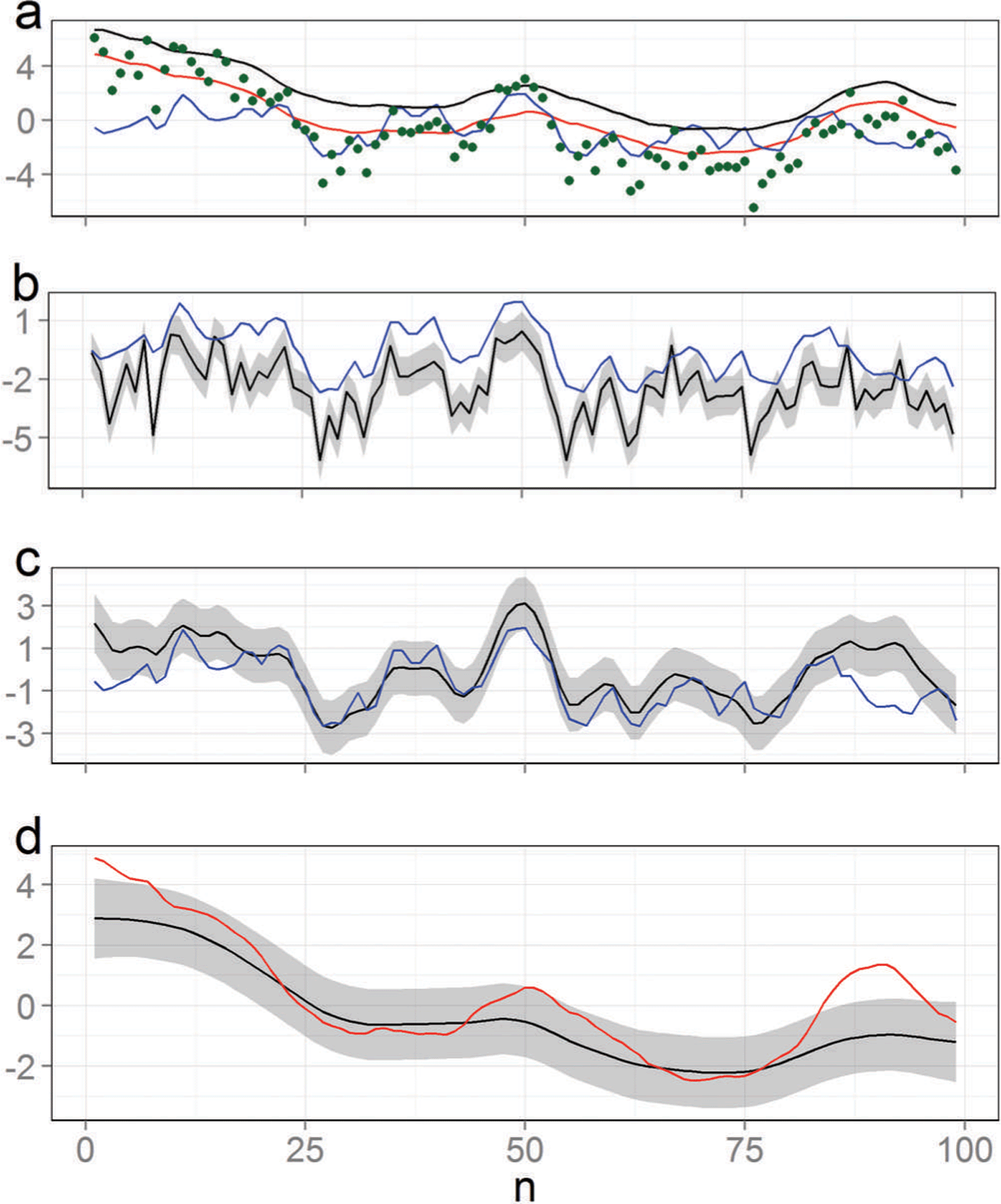
Methods 1–3 (above) ignore the prior information and in the most restrictive case would apply Eqn (3) to subtract a geophysical model output, , from y in order to estimate x ₂. If there is a systematic bias in the model output for x ₁, or a cluster of errors, this will go unnoticed and propagate into our estimate of x ₂ (Fig. 1b). If, though, we also attempt to estimate x ₁ from the data, we increase the flexibility of the possible solutions (and hence the uncertainty) but are more robust to biases and error clusters (Fig. 1c and d). Further, we observe that our uncertainty is dominated by our ability to separate the signals, giving a more complete and reliable approach to uncertainty analysis. For example, the error band on x ₂ is relatively smooth as low-frequency uncertainty from x ₁ is filtering through (Fig. 1c). Probabilistic updates automatically cater for statistical confounding: if we assume that both signals exhibit identical smoothness characteristics then the update will inflate the uncertainty accordingly. Indeed, this extreme case will result in considerable uncertainty even in the presence of accurate observations. Smoothness is not the only property which can be exploited to arrive at a model-free framework for source separation in the context of the AIS. We consider some more approaches in the next section.

Application to Antarctica

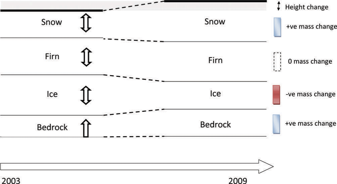
We can view the datasets available for studying the AIS as recordings of elevation (or mass) changes occurring due to four processes: (1) GIA ( x ₁), (2) ice dynamics ( x ₂), (3) firn compaction ( x ₃) and (4) SMB anomalies ( x ₄). As a result of the under-determined nature of the problem, the cause of the observed change is not straightforward (Fig. 2). However, we can use source separation ideas to isolate the causes, even though the number of observation types employed is less than the number of processes under consideration, in this case four.

Fig. 2.

The under-determined nature of the problem of estimating the mass balance of the AIS. Between 2003 and 2009 all salient processes contribute to an overall observed height change and mass change. Source separation is the process by which the individual components are extracted from the observed superpositions. ‘+ve’ and ‘–ve’ are shorthand for positive and negative, respectively.

The method relies on configuring the covariance matrices of x ₁, ..., x ₄ ( Σ ₁, ..., Σ ₄) appropriately, and this is where numerical models can play a role. Even though it is possible that these models exhibit biases and error clusters, there is a broader confidence in their second-order properties. For example, RACMO2.1 simulates the SMB anomaly patterns with relatively low frequency variability in the interior of the continent and higher frequency at the coast. This conforms with in situ observations and also with theoretical considerations of how precipitation varies at continental scales.

Similarly, most GIA models (e.g. ICE-5G (Reference PeltierPeltier, 2004), W12a (Reference Whitehouse, Bentley, Milne, King and ThomasWhitehouse and others, 2012) and IJ05_R2 (Reference IvinsIvins and others, 2013)) agree that GIA is a low-frequency process (with length scales ~1000 km). We can quantify these beliefs by applying standard spatial statistical tools to extract length scales from these models, and then use these to configure the covariance matrices (Reference CressieCressie, 1993; Reference Zammit-Mangion, Rougier, Bamber and SchoenZammit-Mangion and others, 2014).

Spatial smoothness is just one characteristic which can aid source separation. In the framework we employ for the AIS we can incorporate other judgments, as follows:

• From RACMO2.1 it is evident that SMB anomalies are largely temporally uncorrelated, while it is well known that changes due to ice dynamics are temporally relatively smooth (Reference Rignot, Velicogna, Van den Broeke, Monaghan and LenaertsRignot and others, 2011). This, in addition to GIA being temporally constant, implies that time plays a key role in aiding source separation.

• Firn compaction is mainly caused by surface snow being buried and compressed by subsequent snowfall. Therefore, the governing equations in firn compaction models result in the two processes being anticorrelated. We quantify this relationship by carrying out a correlation analysis on the model outputs to measure the extent of interaction, a priori, between these two processes. This correlation can then be incorporated into a cross-covariance matrix across x ₃ and x ₄, i.e. a matrix which defines correlations in space, time and between the two processes.

• All models provide information on the expected amplitude of the changes. For example, GIA is constrained to be small (a few mm a⁻¹) whilst SMB anomaly patterns are constrained to be small in the interior but allowed to be large on the coast. For ice dynamics we can use horizontal ice velocity measurements from interferometric synthetic aperture radar (InSAR; Reference RignotRignot and others, 2008) as auxiliary information. Where ice is flowing slowly we constrain height loss due to ice dynamics to be small (up to 1 cm a⁻¹) but allow it to be large at higher speeds (up to 10 m a⁻¹). Note that, unlike Reference RivaRiva and others (2009), these are soft constraints: the resulting inferences for the update on x can still have a nonzero probability above these thresholds if there is strong evidence for this in the data.

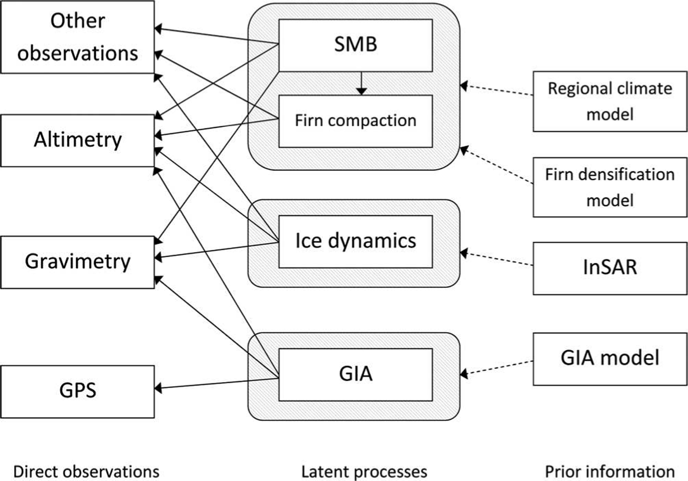
A schematic of the framework applied to the AIS is shown in Figure 3, where the arrows illustrate the direction of information flow. Numerical models and auxiliary datasets are used to implement a prior judgment on the processes, which are then observed using a variety of techniques.

Fig. 3.

Information flow diagram for source separation in the AIS. The prior information (on the right) is used to configure the covariance matrices for the latent processes, x ₁, ..., x ₄, which are then observed using altimetry, gravimetry, GPS and possibly other techniques (e.g. accumulation radar, ‘coffee-can’ point measurements and shallow ice-core data). We use one box to outline the SMB anomaly and firn compaction processes since these interact.

Flexibility of the Approach

The observation equation (e.g. Eqn (1)), and the prior judgments on x ₁, ..., x ₄, constitute a two-level hierarchical framework with immense flexibility from a data-assimilation perspective (Reference Cressie and WikleCressie and Wikle, 2011). Multiple observations can be included by simply defining the relationships between the observations and the acting processes, relationships which can be both spatially varying and contain uncertainties of their own. Consider a spatial-only example. Defining x _i = (X_i(s _j): j = 1, ..., n^T as the height rate due to process X_i (s) at n spatial locations, s _j , then the altimetry observation equation is simply an extension of Eqn (1):

(4)

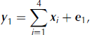
i.e. a rate obtained from a satellite altimeter, such as that on the Ice, Cloud and land Elevation Satellite (ICESat), is a linear superposition of the height rates due to all four processes.

The relationships could be arbitrarily complex. For GRACE mass concentrations (Reference Luthcke, Sabaka, Loomis, Arendt, McCarthy and CampLuthcke and others, 2013), the observation equation for the jth observation is

(5)

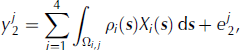
where the integral is needed because each mass concentration is a spatial average over the sum of processes over some domain, Ω _i,j ·ρ_i ( s ), the density of change due to the ith process (e.g. 917 kg m⁻³ for ice dynamics), is required to convert the height rate to the observed mass rate. Ω _i , _j denotes the domain of the integral, and, for i = 2, 3, 4, is defined as the union of the jth mass concentration area and land area within the grounding line (since ice height changes that are seaward of the grounding line do not alter the geoid). For GIA (i = 1), Ω _i , j is just the domain of the mass concentration.

These two examples illustrate the flexibility of the approach. In the example discussed in the Results section, we only use GRACE, altimetry and GPS; however, it is straightforward to include other observations (e.g. snow radar (Reference MedleyMedley and others, 2013), ground-penetration radar (Reference Sinisalo, Grinsted, Moore, Karkas and PetterssonSinisalo and others, 2003), coffee-can measurements (Reference Arthern, Vaughan, Rankin, Mulvaney and ThomasArthern and others, 2010), ice-core data (Reference KaspariKaspari and others, 2004), etc.). One advantage of this flexibility is the possibility to easily add or remove data in order to assess their effect on the estimates and the errors. A further advantage of the two-level hierarchy is the dissociation of the scales of the modelled processes from those of the observations. Pre-smoothing Gaussian filters (Reference RivaRiva and others, 2009; Reference GunterGunter and others, 2014) are no longer necessary and observations can be spatially (and temporally) irregular.

In addition, the algorithms required to evaluate interesting quantities, such as the updates on each of the x _i , do not require a Monte Carlo approach and are thus highly computationally efficient. State-of-the-art algorithms we can use (e.g. those discussed by Reference Rue and HeldRue and Held, 2005) scale approximately linearly with the number of observations and sub-cubically with the resolution of the inferred processes (i.e. the combined dimensionality of ( x ₁, ..., x ₄)). For example, using ICESat, EnviSat and GPS rates on a 20 km grid and 1 year resolution for 2003–09, and a combined dimensionality of 80 000, we are able to construct ice-sheet-wide inferences in <2 hours on a high-end desktop computer. Inclusion of GRACE would require ~1 day and a high-memory machine, due to the added complexity of including the integrals in Eqn (5). However, ice-sheet-wide inferences are not always required; with this framework we can carry out inferences at any scale (e.g. basin or sector scale). In such cases, inferences can be produced in a few minutes with moderate memory requirements. Computational details are provided by Reference Zammit-Mangion, Rougier, Bamber and SchoenZammit-Mangion and others (2014).

Software Implementation

Probabilistic smoothing is a long-standing, accepted approach to signal analysis and uncertainty quantification. However the specific complexities pertaining to the large-scale nature of the AIS require the application of several numerical and approximation routines. Thus, to facilitate the implementation we have developed a package in R Software (R Core Team, 2012) so that analyses can be made with relatively little effort. The package, MVST (multivariate spatio-temporal) incorporates all the necessary routines to study a general multivariate spatio-temporal system, such as that described above. This package, together with two tutorial vignettes (one replicating the toy study above), is available from github.com/andrewzm/MVST.

MVST sets the problem into an object-oriented framework. Each node in the two-level hierarchy (first two columns in Fig. 3) can be constructed as an object, and linked as necessary. The observational inputs are created using the Obs function and, for point datasets, users are only required to provide a text file containing the location, x, y, the observed rate, z, time, t, and the uncertainty, std. Class-specific methods also allow for elementary preprocessing options, such as threshold limits and mean/median averaging over a larger area (e.g. Reference Rue and HeldRue and Held, 2005). Observation polygons for mass concentrations (required to implement Eqn (5)) can be included with the function Obs_poly. In this case the user is also required to specify in a text file points on the polygon which accurately describe the footprint of the observation with fields x1, y1, x2, y2,....

The physical process blocks ( x ₁, ..., x ₄, equating to the four latent processes in Fig. 3) are set up using a function which takes as arguments information on the length scales, dynamics, inter-process correlation and expected amplitudes of the processes. The resolution of each latent process is determined by variable density finite-element triangulations (Fig. 4). MVST provides functions to easily attribute characteristics to both observation and latent process blocks, which could be used for both application of prior judgment and for result generation. These attributes could be information relating to horizontal ice velocity, basin numbers, topography, etc. All auxiliary data need to be specified on a grid, x, y, and contain the dependent variable under z.

Fig. 4.

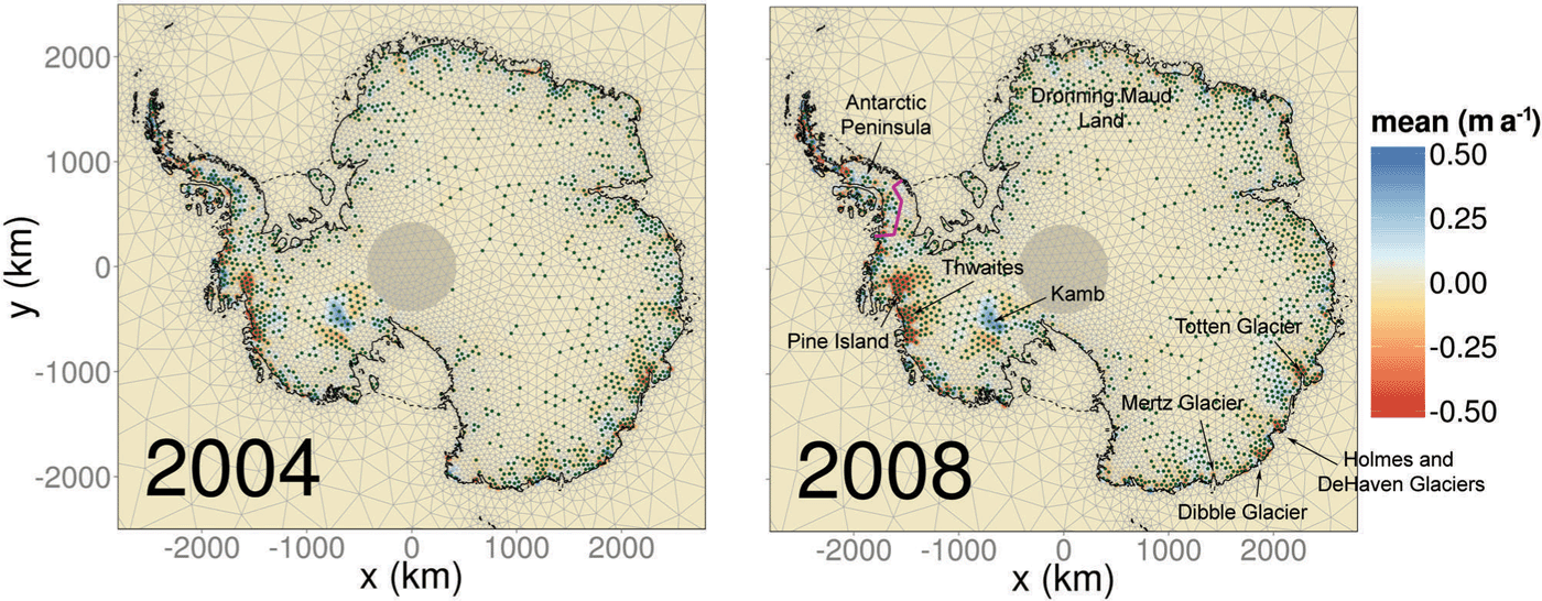
Estimated height rates due to changes in ice dynamics in 2004 and 2008. Each vertex of the triangulation consists of one element of x , and stippled points mark where the updated absolute expectation is greater than the updated 1 σ uncertainty. The coastline and grounding line are denoted by the dashed and solid curves, respectively. The purple curve demarcates the approximate Antarctic Peninsula/West Antarctic ice sheet divide, while the shaded circle at the pole is the ICESat pole gap.

Once observation and latent process objects are constructed, these can be linked together using the function link. Denote the latent processes as ice, surf_firn and GIA. Then, if we want to infer mass balance using ICESat alone we can define the links simply as follows:

L1 <- link(ice,ICESat)

L2 <- link(surf_firn,ICESat)

L3 <- link(GIA,ICESat)

If we assume that GPS is only measuring GIA, we can also include a link

L4 <- link(GIA,GPS)

Other options in the link function are available for observations with large footprints (such as GRACE), including options which specify the resolution at which the integration in Eqn (5) is carried out, and the spatially varying factors with which to convert the height to observed mass change. Once all the links are specified, they are passed on to a routine, Infer, which implements the update and returns the appropriate results: the spatio-temporal posterior expectation and uncertainty of each process.

Illustrative Results

We illustrate the probabilistic smoother and the software packages by using them to carry out inferences on the height rate due to each of the four latent processes (Fig. 3) using height and mass rates obtained from ICESat, EnviSat, GPS and GRACE data between 2003 and 2009.

ICESat data were preprocessed (as by Reference SørensenSørensen and others, 2011) and corrected for both inter-campaign (Reference Hofton, Luthcke and BlairHofton and others, 2013) and centroid Gaussian bias (Reference Borsa, Moholdt, Fricker and BruntBorsa and others, 2014). Due to relatively poor temporal resolution, dh=dt was extracted over 3 year moving windows in 1 km gridboxes adjusted for spatial slope. For example, the rate and uncertainty in 2005 was found by fitting a three-dimensional hypersurface in (x, y, t) through altimetry points between 2004 and 2006 and extracting the rate and uncertainty on the third slope coefficient (Reference Moholdt, Nuth, Hagen and KohlerMoholdt and others, 2010). Rates were also extracted from EnviSat data (Reference Flament and RémyFlament and Rémy, 2012), by fitting a least-squares trend using a 3 year sliding window. All altimetry data was subsequently averaged on a 20 km grid (as Reference RivaRiva and others, 2009).

For GRACE we used the mass concentration solution of Reference Luthcke, Sabaka, Loomis, Arendt, McCarthy and CampLuthcke and others (2013), and fitted rates to each mass concentration on a yearly interval following deseasoning for 2004–09. Data for 2003 were omitted on the recommendation of S.B. Luthcke (personal communication, 2014), due to issues with the level-1 processing for that year. We used two GPS datasets, that of Reference ThomasThomas and others (2011) adjusted for elastic correction and an updated version of this. With the latter dataset, for stations without major gaps or discontinuities, annual trends were derived by fitting a piecewise-linear function. For the other stations we fitted a linear trend over the whole period available and derived error estimates using the GPS coordinate time-series analysis software (CATS; Reference WilliamsWilliams, 2008). No elastic correction was applied to these data, which might influence our results. Below we focus on illustrating some of the key features of the approach. Results using a more complete dataset, including solid-earth elastic corrections and further improvement of GRACE arc parameterizations, will be reported elsewhere. Replication code for this study is available from http://www.rates-antarctica.net/home/software.

Validation of numerical models

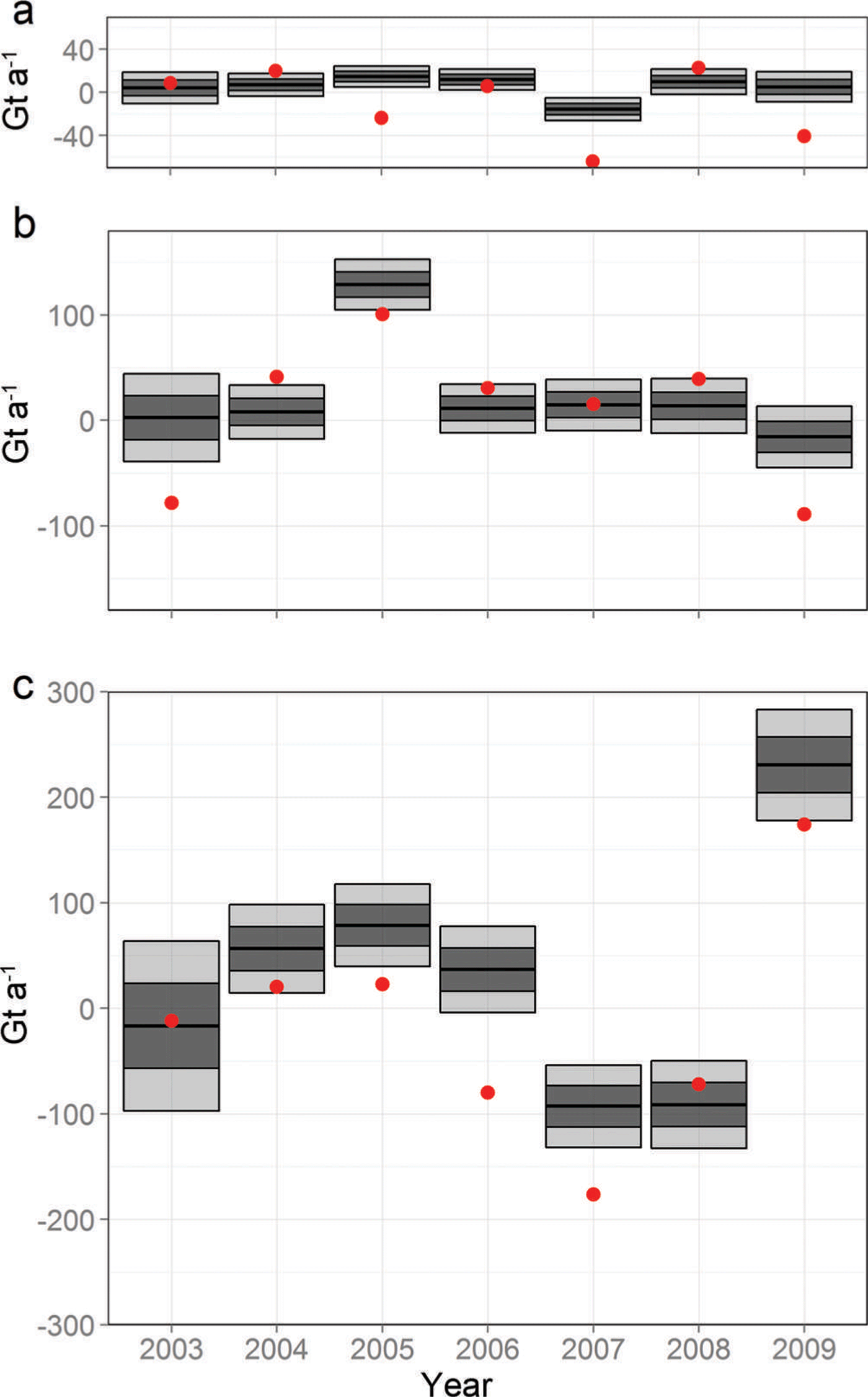
An advantage of a data-driven approach is the possibility of validating numerical models. We compare results for SMB anomalies obtained using our method with RACMO2.1 in Figure 5. We see that, although frequently outside our credibility intervals, our SMB anomaly estimates largely conform with those given by the numerical model. In particular, the well-known positive anomalies in 2009 in Dronning Maud Land (Reference Boening, Lebsock, Landerer and StephensBoening and others, 2012) and in 2005 in the West Antarctic ice sheet (Reference MedleyMedley and others, 2013) are correctly attributed to SMB anomalies (and not ice dynamics or GIA). Interestingly, there is seen to be a systematic difference between our estimates and the output of RACMO2.1 in the Antarctic Peninsula (AP) and the East Antarctic ice sheet (EAIS). Discrepancies in the AP might be due to our set-up. Describing process characteristics in the AP is difficult due to the geographical nature of the area; process information is captured on the triangulated mesh which is hard to construct on a narrow stretch of land. In the EAIS, the difference could be due to the systematic underestimation of SMB by RACMO2.1 (e.g. Reference Van WessemVan Wessem and others, 2014). Alternatively, our approach could be compensating for an overall negative GIA signal detected in the EAIS, similar to that reported by Reference IvinsIvins and others (2013). Distinguishing between SMB anomalies and GIA is particularly difficult in the continent’s interior, since the length scales, and the expected contribution to the GRACE signal by these two processes are similar; thus the time-invariant components of these processes cannot be separated. However, uncertainty arising from confounding due to this similarity is incorporated in our uncertainty estimates. Note how the uncertainty in 2003 is larger than in the other years due to the omission of GRACE data for this year; inferences in 2003 are due to altimetry data, GPS data and information borrowed from estimates in the other years (on which GRACE does have an influence).

Fig. 5.

Estimated rate of mass change (i.e. due to a change from a mean state that results in a zero imbalance) due to surface processes (black bars) and the values given by RACMO2.1 (red dots) for (a) the Antarctic Peninsula, (b) the West Antarctic ice sheet and (c) the East Antarctic ice sheet. The 1 and 2 levels are denoted by the dark and light shading, respectively.

Time-evolving mass-balance estimates

Once we have evaluated an update on x , it is relatively straightforward to compute means and uncertainties over linear combinations of the components of x (e.g. over a basin, across multiple processes or across multiple years). For instance, the mass budget for the West Antarctic ice sheet (WAIS) can be found by summing the mass contribution of changing ice dynamics and SMB anomalies (but not firn compaction or GIA), while the uncertainty can be found by summing over the associated sub-matrix of the updated Var( x ). We show results for this approach compared to the mass-budget method (method 2) results of Reference ShepherdShepherd and others (2012) in Figure 6. The results corroborate each other to a large extent, with the mass- budget method reporting slightly more negative results in the WAIS and the AP.

Fig. 6.

Mass-balance estimates (black) compared with those from the mass-budget method (pink), as reported by Reference ShepherdShepherd and others (2012) for (a) the Antarctic Peninsula, (b) the West Antarctic ice sheet and (c) the East Antarctic ice sheet. The 1 and 2 levels are denoted by the dark and light shading, respectively.

The overall mass balance estimated by our method for the whole AIS from 2003 to 2009 is −38 ± 32 Gt a⁻¹. This lies, as expected, between the ICESat-based estimate of 21 ± 81 Gt a⁻¹ (method 1) and the GRACE-based estimate (method 3) of –57 ± 50 Gt a⁻¹, as reported by Reference ShepherdShepherd and others (2012) between October 2003 and December 2008. Our estimate is higher than that of Reference IvinsIvins and others (2013), who estimated −57 Gt a⁻¹ from 2003 to 2012 using method 3 with the IJ05_R2 model, and considerably higher than the recent empirical estimate of Gunter and others (2013) of −100 ± 44 Gt a⁻¹ for a similar time frame (February 2003–October 2009). The latter result is attributed to a strong positive empirical GIA signal in the WAIS, which was not observed in our solution. Our estimate of the mass balance in the WAIS and AP combined over these years is −53 ± 14 Gt a⁻¹; this is slightly less than, but within error of, that obtained using spatial-only models (−76 ± 15 Gt a⁻¹; Reference Schön, Zammit-Mangion, Bamber, Rougier, Flament, Rémy and LuthckeSchön and others, 2014).

Conclusion

We show that the time-evolving mass balance of an ice sheet can be predominantly data-driven, provided that the numerical models incorporating prior judgment are broadly reliable in terms of characterizing spatial and temporal variability. SMB, firn densification and GIA models play an important role, by providing the required length scales (in both space and time), smoothness and expected amplitude changes, as do auxiliary datasets, such as ice surface velocities which help to weakly constrain the inferences on ice dynamics. We show that the approach is amenable to diverse classes of observations, such as altimetry and satellite gravimetry with large spatial footprints. Relatively constrained uncertainty intervals in the illustrated results show that the method goes a long way to solving the source separation issue in a systematic, repeatable and rigorous approach. In doing so, marginal estimates on each of the processes are obtained which, in turn, can be used to validate numerical models and hence other published results. To facilitate the application of this method to other ice sheets, and to expedite the addition of other observables into the framework, we have developed an R Software package, MVST, which is available from https://github.com/andrewzm/MVST.