Nomenclature
 ${H_l}(q)$
the links’ inertia matrix
- $C(q,\dot q)$
the matrix related to Coriolis and centrifugal efforts
- $q,\dot q,\ddot q$
generalised position, velocity and acceleration vector of links
- ${{\theta }},{{\dot \theta }},{{\ddot \theta }}$
generalised position, velocity and acceleration vector of actuators
- ${H_m}$
the actuator inertia matrix
- ${\bf{\tau }} \in {R^n}$
the elastic torques vector between motors and manipulator’s links
- ${{\bf{\tau }}_{fr}} \in {R^n}$
non-linear friction torque
- ${{\bf{\tau }}_m} \in {R^n}$
the control input torques vector of the actuator
- ${B_i}$
the viscous friction coefficient
- ${F_{ci}}$
the Coulomb friction-related parameter
- ${F_{si}}$
the static friction-related parameter
- ${F_{{\bf{\tau }}i}}$
a positive parameter corresponding to the Stribeck effect
- ${F_{ui}}$
the position dependency of friction and various friction modeling errors
- ${\hat B_i}$, ${\hat F_{ci}}$, ${\hat F_{si}}$ and ${\hat F_{{\bf{\tau }}i}}$
the nominal values of
${B_i}$, ${F_{ci}}$, ${F_{si}}$ and ${F_{{\bf{\tau }}i}}$- $P \in {R^r}$
the vector of manipulator parameters
- $Y(q,\dot q,\ddot q)$
a known regressor matrix
- $K$
the stiffness coefficient
- $h$
a sufficiently smooth function
- ${{\mu }}$
the small enough perturbation coefficient
- ${{\bf{\tau }}_s}$
the control input torque of the slow subsystem
- ${{\bf{\tau }}_f}$
the control input torque of the fast subsystem
- ${\bf{\tau }}_f^*$
the control input torque of the refactored fast subsystem
- ${{{\bar \tau }}_s}$
the corrective slow subsystem control input torque
- ${{{\bar \tau }}_f}$
the corrective fast subsystem control input torque
- ${{\bf{\tau }}_1}$
the corrective control term
- $s$
sliding surface
- $e$
trajectory tracking error
- $\dot e$
velocity tracking error
- ${q_d}(t)$
desired trajectory
- ${h_i},{\bf{\varepsilon }}_{pvn}^i,{{\bf{\varepsilon }}^i},{{\bf{\rho }}_{fi}}$
unknown constants
- ${\lambda _c},{K_s},{\bf{\Lambda }},{w_{1i}},{w_{2i}}$
positive constants
- $v \in {R^n}$
the approximate differential signal
- $\varphi $
an introduced auxiliary variable


1.0 Introduction
As humanity’s exploration of space continues, space manipulators play pivotal roles in space exploration, adept at various on-orbit services like capturing satellites and space debris, [Reference Zhou, Luo and Wang1, Reference Wei, Long, Shi and Song2] Fig. 1. Representative examples include Canadarm2, a key component of the International Space Station (ISS), which has demonstrated exceptional capabilities in module installation, payload handling, and assisting astronauts during extravehicular activities. With its seven-joint design and end-over-end walking capability, it can traverse the ISS structure to perform complex operations [Reference Doetsch34]. Similarly, Redwire’s STAARK is a next-generation modular autonomous robotic arm developed for the maintenance and assembly of small spacecraft. It supports modern on-orbit missions including rendezvous, docking and modular payload handling in both geostationary orbit (GEO) and low-earth orbit (LEO), and is also being prototyped for use with the Argonaut lunar lander, extending its application to future lunar missions [35]. These manipulators not only enhance mission efficiency but also significantly reduce the risk associated with astronauts leaving the capsule. The European Robotic Orbital Support Services (EROSS) represents a landmark initiative in space manipulators, designed to demonstrate next-generation technologies for critical on-orbit servicing operations encompassing propellant replenishment, modular component replacement, and in-situ maintenance. By integrating high-precision robotic arms, sophisticated guidance and navigation systems, and autonomous control algorithms, EROSS enables the safe capture and manipulation of client satellites. This significantly enhances the operational capabilities of robotic systems in space while improving the autonomy and reliability of future orbital servicing missions [Reference Dubanchet, Romero and Gregertsen36]. Generally, lightweight and long-reaching manipulators are favoured to minimise launch mass and expand operational workspace. Nevertheless, a significant issue with such lightweight space manipulators is the increased link flexibilities, which result in structural vibrations, particularly when handling heavy payloads. Additionally, joint flexibilities, which are mostly brought on by harmonic drives, could impact space manipulators [Reference Talole, Kolhe and Phadke3].
A space manipulator operating on-orbit.

This paper focuses on considering joint flexibilities solely. For space manipulators, like the free-floating/flying space manipulator systems under investigation, or for flight systems in previous and ongoing on-orbit services missions such as deutscher orbital service system (DEOS) [Reference Rupp, Boge, Kiehling and Sellmaier4] and e. Deorbit [Reference Jaekel5], the assumption is reasonable. Such flexibilities can lead to substandard performance when handling heavy payloads, potentially causing elastic deformation and system vibration. These issues have a negative impact on the trajectory tracking precision and quicken the wear and tear of flexible components. Additionally, the strong coupling between joint friction and joint flexibility becomes more pronounced, amplifying the nonlinear features of joint friction when space manipulators move at low speed. This exacerbates control challenges, rendering the space manipulators less effective in their operations. To achieve highly accurate trajectory tracking, it is crucial to concurrently consider the impacts of joint flexibility and joint friction.
The dynamics modeling and control problems have been the main topics of previous research on space manipulators with flexible joints. In practical engineering applications, obtaining an accurate mathematical model of a space manipulator poses significant challenges. It is necessary to introduce reasonable approximations during the modeling process to account for uncertainties in certain system parameters. Considering these parameter uncertainties, advanced adaptive control strategies can be employed. Adaptive control techniques mitigate the effects of model parameter uncertainties on control performance by dynamically adjusting parameters in real-time. This approach ensures system asymptotic stabilisation or that steady-state tracking errors tend towards zero, without requiring high gain conditions. Several adaptive control strategies, as detailed in references [Reference Jin, Lee and Tsagarakis6, Reference Ma, Zhou, Li and Lu7], have been proposed, specifically addressing the issue of parametric uncertainties through adaptive techniques. A fully dynamic feedforward compensation component and a PD feedback component comprise the computationally straightforward and efficient adaptive tracking controllers that Slotine and Li presented [Reference Slotine and Li8]. Online parameter estimation is used to determine the payload and unknown manipulator. To mitigate the elastic oscillation at the joints, Spong introduced a straightforward correction term to the controller for manipulators and provided a new singular perturbation-based adaptive controller for a flexible-joint manipulator [Reference Spong, Khorasani and Kokotovic9, Reference Spong10]. The adaptive compensation control method that Huang et al. described enables precise trajectory tracking and the limited torque errors for a flexible joint manipulator with limited mobility and uncertain parameters [Reference Huang, Ge and Lee11]. The controller uses joint state variables feedback, avoiding the commonly found noisy joint torque measurements in other controllers. Moreover, some researchers combined fuzzy and neural network with adaptive control law to propose compensatory control approaches for flexible-joint manipulators. To address the model uncertainties, Subudhi and Morris proposed a strategy in which the radial basis function neural network was used for the slow control and a linear-quadratic fast control [Reference Subudhi and Morris12]. As research continues to progress, extended adaptive control schemes are provided. The provided adaptive controller compensates for the friction brought on by harmonic drives, while considering the dynamic characteristics of the joint flexibility. However, methods take only static friction into account [Reference Zhu, Dupuis and Doyon13, Reference Le-Tien and Albu-Schäffer14]. The space manipulator’s dynamic model considering joint friction was provided by Zhang et al., employing the single direction recursive construction method and Jourdain’s velocity variation concept. By utilising the computed torque approach, a trajectory tracking control strategy that includes friction compensation is proposed [Reference Zhang, Liu and Cai15].
Recently, innovative control strategies have been developed to address the challenges posed by hybrid uncertainties in vibration active control systems. For instance, Li et al. proposed a proportional–integral–derivative (PID) controller design based on probability density evolution method and interval-oriented sequential optimisation strategy [Reference Liu, Wang and Wu37], which effectively handles both interval and random uncertainties. This approach not only enhances the reliability of the control system but also balances energy consumption and safety. Similarly, Wang et al. introduced a Kriging-based decoupled non-probability reliability-based design optimisation scheme for piezoelectric PID control systems [Reference Wang, Zhao and Liu38]. This method decouples uncertainty parameters and design variables, significantly improving computational efficiency while maintaining accuracy. These advancements highlight the ongoing efforts to enhance control strategies for systems with complex uncertainties.
Joint friction is initially described utilising the Coulomb friction model. Subsequently, various models have been developed, including the LuGre model, which effectively captures most friction behaviour [Reference Wu16]. The literature has taken the combined influence of joint flexibility and friction into consideration. Research has concentrated on identifying and compensating for joint friction in a manipulator. The friction compensation algorithm is composed of a single-state dynamic model that describes the friction torque [Reference Zhang, Liu and Cai17]. An adaptive control strategy was provided by M. Feemster to compensate for linear parametric friction in a second-order mechanical system that includes frictional effects such as Coulomb, static, Stribeck and viscous friction. The Stribeck parameter is assumed to be accurately known [Reference Zhang and Yuan18]. For the complicated friction features, H. Gao constructed a precise and effective hybrid friction model incorporating static, Coulomb and Stribeck friction, where velocity acts as the determining factor for switching between friction types [Reference Gao, Li, Guan and Hao19]. Although the previous control laws can effectively achieve accurate tracking of positions and mitigate structural vibration for flexible joint space manipulators, there are currently few control strategies designed to compensate joint friction for flexible joint space manipulators. It is challenging to carry out position tracking control and vibration suppression rapidly and accurately because joint flexibility can cause oscillation, and joint friction may reduce tracking efficiency.
The primary contributions of this paper are that an adaptive control strategy based on singularly perturbed decoupling is provided for flexible-joint space manipulators to mitigate joint flexibility and address nonlinear joint friction issues when parametric uncertainties and joints friction are present. This control strategy consists of the following three primary parts:
1. A novel decomposition-based friction compensation scheme is designed to compensate for joint friction.
2. A modified compensation scheme is proposed to solve the problem that the conventional singular perturbation method is limited to be utilised in space manipulators with weak joint flexibility.
3. A composite adaptive control scheme according to singular perturbation decoupling is proposed to compensate for joint flexibility.
A nonlinear experimental friction model is linearised in parameters to provide a linear parametric friction model, which describes joint friction. The friction compensator is designed with the compensation control scheme based on decomposition. The essential principle of the decomposition-based modeling and control strategy lies in distinguishing between different types of uncertain parameters and variables, designing separate compensators for each, and considering each physical characteristic. The strategy aims to deal with various kinds of model uncertainty in appropriate way, which makes it possible to target different types of friction characteristics more precisely. The performance of mechanical systems under friction model uncertainty can be significantly enhanced by employing a combination of adaptive and robust compensators.
The singular perturbation technique is a highly effective method for managing complex systems with multi-scale features. Since M.W. Spong first demonstrated its feasibility for modeling and control, it has been widely applied in the study of flexible joint space manipulators. This approach offers the advantage of model reduction, decomposing the original high-order system into two low-order subsystems. This decomposition facilitates the design of corresponding controllers, simplifies the overall control strategy design process, and allows for detailed dynamic analysis of each subsystem. However, the conventional singular perturbation method is typically suitable solely for manipulators with weak joint flexibility. A modified compensation scheme is proposed to enhance system stiffness and address deviations, thereby overcoming the limitations imposed on traditional singular perturbation methods. This enhancement is achieved by incorporating a compensation term into the control law. According to the concept of integral manifolds, this compensation term is designed to improve system stiffness, enabling the control system to manage joint flexibility more effectively.
To compensate for joint flexibility, a composite controller is designed for flexible joint space manipulators. The inertias of the rotors, including gear reduction, which have often been neglected in previous research, are taken into account in the process of modeling the dynamics in this paper in order to build a more accurate dynamics model. By introducing the concept of integral manifolds, the two subsystems, fast and slow, obtained based on singular perturbation decoupling are refactored into two different tracking systems, which facilitates the development of the system control approach. First, for the slow subsystem, an adaptive control scheme with friction compensation is designed, employing an enhanced linear parameterisation expression. This approach aims to improve parametric estimation accuracy by minimising distortion in the linearity model. On the other side, different from the methods in previous research, by reconfiguring the fast subsystem into a tracking system, i.e. making the real elastic torque track the desired elastic torque, the elastic torque error tends to zero and is not explicitly expressed in the fast subsystem, which allows for greater flexibility in the design of control strategy for the fast subsystem [Reference Spong, Khorasani and Kokotovic9, Reference Spong10, Reference Khosravi and Taghirad20]. Additionally, the Lyapunov theorem is utilised to demonstrate that the entire control system is asymptotically stable.
The remains are structured as follows: Section 2 provides the dynamics of the flexible-joint space manipulators and the friction model parameters. In Section 3, the dynamic system of space manipulators with flexible joint is decomposed into two second-order subsystems with distinct time scales utilising singular perturbation theory. Next, an adaptive controller is designed in Section 4, which is followed by the stability proof according to the Lyapunov stability theorem of the provided control strategy in Section 5. In Section 6, numerical simulations and comparable analysis for a 3-linked flexible joint space manipulator are presented. Finally, Section 7 provides conclusions, while Section 8 outlines the future work.
2.0 Dynamic Modeling
The following describes the established dynamic model of a space manipulator with flexible joint: [Reference Ruderman21, Reference Ulrich and Sasiadek22]
 \begin{align}{H_l}(q)\ddot q + C(q,\dot q)\dot q = {\bf{\tau }}\end{align}
 \begin{align}{H_m}{{\ddot \theta }} + {\bf{\tau }} + {{\bf{\tau }}_{fr}} = {{\bf{\tau }}_m}\end{align}
 \begin{align}{\bf{\tau }} = K({\bf{\theta }} - q)\end{align}
 ${H_l}(q)$ and
 $C(q,\dot q)$ are substituted with
 ${H_l}$ and
 $C$, respectively, to simplify the formulations.
According to various space studies conducted thus far, joint friction appears to be more pronounced in space than on Earth. In this paper, for analytical ease and without sacrificing generality, the mathematical model of joint non-linear friction  ${{\bf{\tau }}_{fr}}$ takes the form [Reference Ahmad23–Reference Liu, Abdul and Goldenberg25].
 \begin{align}{{\bf{\tau }}_{fr}} = {B_i}{\dot q_i} + [{F_{ci}} + {F_{si}}\exp ( {-} {F_{{\bf{\tau }}i}}{\dot q_i}^2)]sign({\dot q_i}) + {F_{ui}}({q_i},{\dot q_i})\end{align}
For the  $i$ joint, where
 ${q_i} \in {R^n}$ and
 ${\dot q_i} \in {R^n}$ represent the position and velocity of the link,
 ${B_i}$ denotes the viscous friction coefficient,
 ${F_{ci}}$ symbolises the Coulomb friction-related parameter,
 ${F_{si}}$ represents the static friction-related parameter,
 ${F_{{\bf{\tau }}i}}$ is a positive parameter corresponding to the Stribeck effect,
 ${F_{ui}}({q_i},{\dot q_i})$ captures the position dependency of friction and various friction modeling errors.
 ${\hat B_i}$,
 ${\hat F_{ci}}$,
 ${\hat F_{si}}$ and
 ${\hat F_{{\bf{\tau }}i}}$ represent the nominal values of
 ${B_i}$,
 ${F_{ci}}$,
 ${F_{si}}$ and
 ${F_{{\bf{\tau }}i}}$, respectively. The definition of the sign function is
 \begin{align}sign({\dot q_i}) = \left\{ {\begin{array}{*{20}{c}}{\begin{array}{*{20}{c}}{ + 1}\\0\\{ - 1}\end{array}} {}{\begin{array}{*{20}{c}}{\begin{array}{*{20}{c}}{{{\dot q}_i} \gt 0}\\{{{\dot q}_i} = 0}\end{array}}\\{{{\dot q}_i} \lt 0}\end{array}}\end{array}} \right.\end{align}
Under the assumption that the nominal values of  ${\hat F_{si}}$ and
 ${\hat F_{{\bf{\tau }}i}}$ are nearly true to their true values, the nonlinear term
 ${F_{si}}\exp ( {-} {F_{{\bf{\tau }}i}}{\dot q_i}^2)$ is linearised at
 ${\hat F_{si}}$ and
 ${\hat F_{{\bf{\tau }}i}}$. Neglecting higher-order terms, the following equation is obtained.
 \begin{align}\begin{array}{c}{F_{si}}\exp ( {-} {F_{{\bf{\tau }}i}}{{\dot q}_i}^2) \cong ({{\hat F}_{si}} + {{\tilde F}_{si}})(\exp ( {-} {{\hat F}_{{\bf{\tau }}i}}{{\dot q}_i}^2) - \exp ( {-} {{\hat F}_{{\bf{\tau }}i}}{{\dot q}_i}^2){{\tilde F}_{{\bf{\tau }}i}}{{\dot q}_i}^2)\\ \cong {{\hat F}_{si}}\exp ( {-} {{\hat F}_{{\bf{\tau }}i}}{{\dot q}_i}^2) + \exp ( {-} {{\hat F}_{{\bf{\tau }}i}}{{\dot q}_i}^2){{\tilde F}_{si}} - {{\hat F}_{si}}\exp ( {-} {{\hat F}_{{\bf{\tau }}i}}{{\dot q}_i}^2){{\tilde F}_{{\bf{\tau }}i}}{{\dot q}_i}^2)\end{array}\end{align}
The linear parameterised friction model can be obtained as follows:
 \begin{align}{{\bf{\tau }}_{fri}} = {B_i}{\dot q_i} + [{F_{ci}} + {\hat F_{si}}\exp ( {-} {\hat F_{{\bf{\tau }}i}}{\dot q_i}^2) + \exp ( {-} {\hat F_{{\bf{\tau }}i}}{\dot q_i}^2){\tilde F_{si}} - {\hat F_{si}}\exp ( {-} {\hat F_{{\bf{\tau }}i}}{\dot q_i}^2){\tilde F_{{\bf{\tau }}i}}{\dot q_i}^2)]sign({\dot q_i}) + {F_{ui}}({q_i},{\dot q_i})\end{align}
The following is a summary of several characteristics of the manipulator’s dynamic model as described in (1), (2) and (3) [Reference Slotine and Li8].
Property 1:  ${\dot H_l}(q) - 2C(q,\dot q)$ is skew-symmetric, satisfying the relationship:
 ${\zeta ^T}[{\dot H_l}(q) - 2C(q,\dot q)]\zeta = 0$,
 $\forall \zeta ,q,\dot q \in {R^n}$.
Property 2: The inertia matrix  ${H_l}(q)$ is symmetric and positive-definite.
Property 3: The Euler-Lagrange dynamics can be expressed in a linearly parameterisable form such that:
 \begin{align}{H_l}(q)\ddot q + C(q,\dot q)\dot q = Y(q,\dot q,\ddot q)P\end{align}
where  $P \in {R^r}$ is the vector of manipulator parameters, and
 $Y(q,\dot q,\ddot q)$ is a known regressor matrix.
3.0 Two-time Scale Decomposition
Applying singular perturbation decoupling, the dynamic model of the flexible-joint space manipulators described in (1), (2) and (3) can be decomposed into two subsystems with distinct time scales. The manipulator discussed in this section has weak flexibility at the joint, that is, the stiffness coefficient  $K$ of the joint is large enough.
All the stiffness coefficients  ${k_i}$ are expressed as a large enough parameter k, provided that they are all of the same order of magnitude [Reference Spong, Khorasani and Kokotovic9].
 \begin{align}{K_i} = k{\tilde K_i},i = 1, \cdots ,n.\end{align}
 $\tilde K = diag\left\{ {{{\tilde k}_1}, \ldots ,{{\tilde k}_n}} \right\}$, to simplify the expression without losing generality,
 $\tilde K = I$.
Equation is derived by substituting equation (3) into the deformed equation (1).
 \begin{align}\ddot q = - {H_l}^{ - 1}C\dot q + {H_l}^{ - 1}{\bf{\tau }}\end{align}
Introducing a minimal parameter  ${{\mu }} = 1/k$, transforming (2) and (9), and then bringing them into (3), equation (11) is obtained.
 \begin{align}{{\mu \ddot \tau }} = {H_l}^{ - 1}C\dot q + {H_m}^{ - 1}{{\bf{\tau }}_m} - ({H_m}^{ - 1} + {H_l}^{ - 1}){\bf{\tau }} - {H_m}^{ - 1}{{\bf{\tau }}_{fr}}\end{align}
The coupled nonlinear system represented by equations (10) and (11) is the singular perturbation system model. Without simplification, it is unlikely to be tractable for analysis or control-system design [Reference Spong, Khorasani and Kokotovic9].
Employing the notion of integral manifold, the elastic torques  ${\bf{\tau }}$ is defined as following formula,
 \begin{align}{\bf{\tau }} = h(q,\dot q,{{\mu }},{{\bf{\tau }}_m})\end{align}
To simplify the expressions,  $h(q,\dot q,{{\mu }},{{\bf{\tau }}_m})$ is substituted with
 $h$. Suppose that
 $h$ is a sufficiently smooth function with regard to the variables
 $q$,
 $\dot q$,
 ${{\mu }}$ and
 ${{\bf{\tau }}_m}$. Expanding
 ${\bf{\tau }}$ in power series,
 \begin{align}{\bf{\tau }} = {h_0} + {{\mu }}{h_1} + {{{\mu }}^2}{h_2} + \cdots + {{{\mu }}^n}{h_n} + \cdots \end{align}
where  ${h_0}$ represents the desired elastic torque,
 ${h_i}$ is an expansion of
 ${{\mu }}$, which can be computed iteratively.
Similarly,  ${{\bf{\tau }}_m}$ expands as follows:
 \begin{align}{{\bf{\tau }}_m} = {{\bf{\tau }}_0} + {{\mu }}{{\bf{\tau }}_1} + {{{\mu }}^2}{{\bf{\tau }}_2} + \cdots + {{{\mu }}^n}{{\bf{\tau }}_n} + \cdots \end{align}
where  ${{\bf{\tau }}_0}$ represents slow subsystem control input torque, namely
 ${{\bf{\tau }}_s}$.
3.1 Slow subsystem
Observe that,  ${{\mu }} \to 0$, i.e.
 $k \to \infty $ will lead to
 ${\bf{\theta }} \to q$ and
 ${\bf{\tau }} \to {h_0}$, thus the control torque
 ${{\bf{\tau }}_m}$ becomes the slow control law
 ${{\bf{\tau }}_s}$. Equations (10) and (11) can be expressed as
 \begin{align}\ddot q = - {H_l}^{ - 1}C\dot q + {H_l}^{ - 1}{h_0}\end{align}
 \begin{align}{h_0} = {({H_m}^{ - 1} + {H_l}^{ - 1})^{ - 1}}({H_l}^{ - 1}C\dot q + {H_m}^{ - 1}{{\bf{\tau }}_s} - {H_m}^{ - 1}{{\bf{\tau }}_{fr}})\\[3pt]\nonumber\end{align}
Substituting equation (16) into equation (15), the slow subsystem is derived as:
 \begin{align}({H_m} + {H_l})\ddot q + C\dot q + {{\tau }_{fr}} = {{\bf{\tau }}_s}\end{align}
where  ${{\bf{\tau }}_s}$ is the slow control input. This subsystem evolves on a time scale
 ${t_{slow}} = O(1)$, determined by the perturbation parameter
 ${{\mu }} = 1/k$. For
 ${{\mu }} = {10^4},{{\bf{\tau }}_f}{\rm{ = }}{10^{{\rm{ - }}4}}$, implying that the slow dynamics dominate below frequencies
 ${\omega _s} = O(1/{t_{slow}}) \approx 1rad/s$. Equation (17) represents the rigid part of the dynamics for a flexible-joint space manipulator, which is practically equal to the model of a rigid manipulator. This equivalence allows for leveraging established control strategies from rigid space manipulators to address the challenges posed by the flexible joint manipulators’ slow dynamics.
3.2 Fast subsystem
The small enough perturbation coefficient  ${{\mu }}$ has its selection rule dependent on K. K needs to be sufficiently large to guarantee that the fast variable is fast enough on a fast time scale
 ${{{\mu }}^{{\bf{ - 1}}}}{\bf{t}}$. However, in practice, K cannot approach infinity and typically has an order of magnitude around 104, i.e.
 ${{\mu }}$ has a value of 10−4. In other words, although
 ${{\mu }}$ is minimal, it cannot be infinitely close to zero. Consequently, ignoring the higher-order term of the h will result in an error, necessitating the implementation of a controller within the fast subsystem to restrain the errors resulting from not taking higher-order terms into account.
Considering the neglected higher-order term of the Taylor series expansion for  ${{\mu }}$ in (13) (used to characterise the flexibility factor in the joint), defining the elastic torque error as
 \begin{align}{\bf{\eta = }}{{{h}}_{{0}}} - {\bf{\tau }}\end{align}
when  $h \to {h_0}$,
 ${{\bf{\tau }}_m} \to {{\bf{\tau }}_s}$, equation (11) can be expressed as
 \begin{align}{{\mu }}{\ddot h_0} = {H_l}^{ - 1}C\dot q + {H_m}^{ - 1}{{\bf{\tau }}_s} - ({H_m}^{ - 1} + {H_l}^{ - 1}){h_0} - {H_m}^{ - 1}{{{\tau }}_{fr}}\end{align}
From equations (11), (18) and (19), the fast subsystem can be derived.
 \begin{align}{{\mu \ddot \eta }} = - ({H_m}^{ - 1} + {H_l}^{ - 1}){\bf{\eta }} - {H_m}^{ - 1}{{\bf{\tau }}_s}\end{align}
Considering equations (18) and (19), equation (20) can be represented as a refactored fast subsystem
 \begin{align}{{\mu \ddot \tau }} = - {H_m}^{ - 1}{\bf{\tau }}_f^* - ({H_m}^{ - 1} + {H_l}^{ - 1}){\bf{\tau }}\end{align}
where  ${\bf{\tau }}_f^*$ symbolises the control input torque of the refactored fast subsystem, and the interconnection between
 ${\bf{\tau }}_f^*$ and
 ${{\bf{\tau }}_f}$ is provided as follows:
 \begin{align}{\bf{\tau }}_f^* = - {{\mu }}{H_m}{\ddot h_0} - {H_m}({H_m}^{ - 1} + {H_l}^{ - 1}){h_0} - {{\bf{\tau }}_f}\end{align}
It’s remarkable that the refactored fast subsystem (21) with a new control objective to control  ${\bf{\tau }}$ tracking
 ${h_0}$ as opposed to (22), which requires the computation of the elastic moment
 ${\bf{\eta }}$ and its second-order derivative term
 ${{\ddot \eta }}$. In other words, the reconfigured fast system controls the fast variable
 ${\bf{\eta }}$ to converge to zero over time without considering it in the system model. This approach makes the design of the fast subsystem more flexible.
3.3 Corrective control term
It is well known that the conventional singular perturbation method is limited to be utilised in space manipulators with weak joint flexibility. Thus, a corrective control law is derived by comparing the equations of the manipulator system with integral flow to those of a fully rigid manipulator. This comparison yields a new control law design architecture that compensates for flexibility and improves system stiffness. Consequently, this corrective approach extends the applicability of the singular perturbation method to manipulators with strong joint flexibility.
Equation (23) is derived by substituting equations (13) and (14) into the equation (11)
 \begin{align}\begin{array}{c}{{\mu }}({{\ddot h}_0} + {{\mu }}{{\ddot h}_1} + {{{\mu }}^2}{{\ddot h}_2} + \cdots + {{{\mu }}^n}{{\ddot h}_n} + \cdots )\\[3pt] = {H_l}^{ - 1}C\dot q + {H_m}^{ - 1}({{\bf{\tau }}_0} + {{\mu }}{{\bf{\tau }}_1} + \cdots + {{{\mu }}^n}{{\bf{\tau }}_n} + \cdots )\\[3pt] - ({H_m}^{ - 1} + {H_l}^{ - 1})({h_0} + {{\mu }}{h_1} + \cdots + {{{\mu }}^n}{h_n} + \cdots ) - {H_m}^{ - 1}{{{\tau }}_{fr}}\end{array}\end{align}
Observing the equation (23), the following conclusions in terms of  ${{\mu }}$ can be obtained.
 \begin{align}0 = {H_l}^{ - 1}C\dot q + {H_m}^{ - 1}{{\bf{\tau }}_0} - ({H_m}^{ - 1} + {H_l}^{ - 1}){h_0} - {H_m}^{ - 1}{{{\tau }}_{fr}}\end{align}
 \begin{align}{\ddot h_{n - 1}} = {H_m}^{ - 1}{{\bf{\tau }}_n} - ({H_m}^{ - 1} + {H_l}^{ - 1}){h_n}\\\nonumber\end{align}
Considering that the perturbation coefficient  ${{\mu }}$ is small enough, equations (13) and (14) can be rewritten as
 \begin{align}{\bf{\tau }} = {h_0} + {{\mu }}{h_1}\end{align}
 \begin{align}{{\bf{\tau }}_m} = {{\bf{\tau }}_0} + {{\mu }}{{\bf{\tau }}_1} = {{{\bar \tau }}_s}\\\nonumber\end{align}
where  ${{\bf{\tau }}_1}$ represents the corrective control term and
 ${{{\bar \tau }}_s}$ represents the corrective slow subsystem control input torque.
Considering equations (24), (25), (26) and (27), equation (10) can be rewritten as
 \begin{align}\begin{array}{c}\ddot q = ( {-} {H_l}^{ - 1}C + {H_l}^{ - 1}{({H_l}^{ - 1} + {H_m}^{ - 1})^{ - 1}}{H_l}^{ - 1}C)\dot q - ({H_l}^{ - 1}{({H_l}^{ - 1} + {H_m}^{ - 1})^{ - 1}}{H_m}^{ - 1}){{\bf{\tau }}_{fr}}\\ - {H_l}^{ - 1}{({H_l}^{ - 1} + {H_m}^{ - 1})^{ - 1}}{H_m}^{ - 1}{{\bf{\tau }}_0} + {{\mu }}{H_l}^{ - 1}{({H_l}^{ - 1} + {H_m}^{ - 1})^{ - 1}}({H_m}^{ - 1}{{\bf{\tau }}_1} - {{\ddot h}_0})\end{array}\end{align}
Meanwhile, the corrective fast subsystem control input torque  ${{{\bar \tau }}_f}$ can be derived by employing equations (14) and (27)
 \begin{align}{{{\bar \tau }}_f} = {{{\mu }}^2}{{\bf{\tau }}_2} + \cdots + {{{\mu }}^n}{{\bf{\tau }}_n} + \cdots \end{align}
Similar to the fast subsystem described in the section 3.2, the corrected fast subsystem equation for the flexible joint space manipulator with strong joint flexibility can be expressed as follows:
 \begin{align}{{\mu \ddot \tau }} = - {H_m}^{ - 1}{{\bar \tau }}_f^* - ({H_m}^{ - 1} + {H_l}^{ - 1}){{\bar \tau }}\end{align}
where  ${{\bar \tau }}_f^*$ symbolises the corrective control input torque of the refactored fast subsystem, and the interconnection between
 ${{\bar \tau }}_f^*$ and
 ${{{\bar \tau }}_f}$ is provided as follows:
 \begin{align}{{\bar \tau }}_f^* = - {{\mu }}{H_m}{\ddot h_0} - {H_m}({H_m}^{ - 1} + {H_l}^{ - 1}){h_0} - {{{\bar \tau }}_f} - {{\mu }}{{\bf{\tau }}_1}\end{align}
As previously mentioned, for the nonlinear flexible joint space manipulator with strong joint flexibility, the dynamics can be decoupled using singular perturbation theory into the corrected slow subsystem equation (28) and the corrected fast subsystem equations (30) and (31).
It is widely accepted that a rigid space manipulator system can be described in the following general form:
 \begin{align}{H_{lr}}(q)\ddot q + {C_r}(q,\dot q)\dot q = {{\bf{\tau }}_r}\end{align}
where  ${H_{lr}}$,
 ${C_r}$, and
 ${{\bf{\tau }}_r}$ are equivalent to
 ${H_l}$,
 $C$, and
 ${\bf{\tau }}$ in Section 2. The equation can be represented as:
 \begin{align}\ddot q = - {H_{lr}}^{ - 1}{C_r}\dot q + {H_{lr}}^{ - 1}{{\bf{\tau }}_r}\end{align}
To ensure that the stiffness of the manipulator system remains sufficiently large after introducing the corrective control term, it is necessary to make the corrected slow subsystem equation (28) in a flexible joint space manipulator with strong joint flexibility as consistent as possible with the equation (33). Hence, the primary function of the corrective control term (34) is to eliminate all relevant terms in equation (28) with respect to  ${{\mu }}$.
 \begin{align}{{\bf{\tau }}_1} = {H_m}{\ddot h_0}\end{align}
4.0 Design of Controller
The fast-slow two-time scale system that is previously presented is obtained by combining the concepts of integral manifolds with singular perturbation theory. The controller design is rendered simplified by this decoupling treatment of the flexible-joint space manipulator’s initial complicated dynamics, permitting separate design and implementation of the sub-controllers for each subsystem.
4.1 Control objective
To ensure precise tracking of the desired trajectory and to effectively mitigate vibrations in flexible joints, the implementation of an appropriate control strategy is crucial. Considering joint friction which can disturb the tracking control, an adaptive control approach with friction compensation to guarantee accurate tracking of positions is proposed.
It is assumed that desired trajectory  ${q_d}(t) \in {R^n}$ is twice differentiable and that
 ${q_d}(t)$ and its first two derivatives are bounded for all
 $t \ge 0$. The control goal of this section is to propose a controller to ensure that the practical trajectory
 $q(t) \in {R^n}$ can asymptotically converge to the desired trajectory
 ${q_d}(t)$. The trajectory tracking error is described as
 $e = q - {q_d}$, the following is the control objective:
 \begin{align}\forall e(0) \in {R^n},\mathop {\lim }\limits_{t \to \infty } e = 0\end{align}
4.2 Slow subsystem controller
To ensure asymptotic convergence of the tracking and eliminate undesirable steady-state position errors, errors are restricted to lie on a sliding surface [Reference Slotine and Li8]
 \begin{align}\dot e + {\bf{\Lambda }}e = 0\end{align}
where the matrix  ${\bf{\Lambda }} \in {R^{n \times n}}$ is constant and its eigenvalues are only found on the complex plane’s right side. Formally, the goal is achieved by substituting the virtual desired trajectory for
 ${q_d}(t)$ in the previous derivation
 \begin{align}{q_r} = {q_d} - {\bf{\Lambda }}\int_0^t {edt} \end{align}
The following definitions are established for the control design:
 \begin{align}{\dot q_r} = {\dot q_d} - {\bf{\Lambda }}e\end{align}
 \begin{align}{\ddot q_r} = {\ddot q_d} - {\bf{\Lambda }}\dot e\end{align}
 \begin{align}s = \dot q - {\dot q_r} = \dot e + {\bf{\Lambda }}e\\[-6pt]\nonumber\end{align}
In general, the slow subsystem linearisation is approximated utilising a parameter linearisation method as for rigid manipulators, which is proposed by Slotine and Li [Reference Slotine and Li8]. However, this method deteriorates the accuracy of the system parameter estimation and introduces modeling error [Reference Raouf, Mohamad, Maarouf and Maamar26]. An enhanced parameter linearisation method is used in the provided control approach to make the approximation more accurate [Reference Liu, Huang and Wu27].
 \begin{align}{H_l}({\ddot q_r} + {\lambda _c}s) + C({\dot q_r}) = Y(q,\dot q,{\dot q_r},{\ddot q_r} + {\lambda _c}s)P\end{align}
 \begin{align}{\hat H_l}({\ddot q_r} + {\lambda _c}s) + \hat C({\dot q_r}) = Y(q,\dot q,{\dot q_r},{\ddot q_r} + {\lambda _c}s)\hat P\\\nonumber\end{align}
where Y is corresponding regressor matrix,  $\hat P$ is the approximation of the manipulator parameter P,
 ${\hat H_l}$ and
 $\hat C$ denote the approximation of
 ${H_l}$ and C,
 ${{\bf{\lambda }}_c}$ is an arbitrary positive constant.
An adaptive controller for the manipulator with weak joint flexibility is proposed as
 \begin{align}{{\bf{\tau }}_s} = ({\hat H_l} + {\hat H_m})({\ddot q_r} + {\lambda _c}s) + \hat C({\dot q_r}) - Ks + F\end{align}
where  $K = {\lambda _c}(M + J) + {K_s}$, of which Ks is positive-definite, and F denotes the friction compensation term.
Define  $(\tilde \cdot ) = (\hat \cdot ) - (\!\cdot\!)$,
 $(\!\cdot\!)$ represents the practical value,
 $(\hat \cdot )$ denotes the approximate value and
 $(\tilde \cdot )$ symbolises the approximation error.
The adaptive control law is proposed as
 \begin{align}\dot{\hat{P}} = - {{\bf{\Gamma }}^{ - 1}}({Y^T}(q,\dot q,{\dot q_r},{\ddot q_r} + {\lambda _c}s)s + {\bf{\Gamma }}\tilde P)\end{align}
where  ${\bf{\Gamma }} \in {R^{n \times n}}$ is a positive-definite constant gain matrix.
Moreover, for manipulators with strong joint flexibility, a corrected control term is proposed to improve system stiffness, enabling the control system to manage joint flexibility more effectively. Employing equations, and, the corrective slow subsystem controller is proposed as
 \begin{align}\begin{array}{c}{{{{\bar \tau }}}_s} = {{\bf{\tau }}_0} + {{\mu }}{{\bf{\tau }}_1} = ({{\hat H}_l} + {{\hat H}_m})({{\ddot q}_r} + {\lambda _c}s) + \hat C({{\dot q}_r}) - Ks + F + {{\mu }}{H_m}{{\ddot h}_0}\end{array}\end{align}
4.3 Friction compensator
According to the friction model of the i joint as equation (4), a decomposition-based compensation scheme is applied to design the friction compensator [Reference Liu28]. Where  $Z({\dot q_i})$ and
 ${}^i\tilde F$ are defined as:
 \begin{align}Z({\dot q_i}) = [{\dot q_i}{\kern 1pt} {\kern 1pt} {\kern 1pt} {\kern 1pt} {\kern 1pt} {\kern 1pt} {\kern 1pt} sign({\dot q_i}){\kern 1pt} {\kern 1pt} {\kern 1pt} {\kern 1pt} {\kern 1pt} {\kern 1pt} {\kern 1pt} {\kern 1pt} {\kern 1pt} \exp ( {-} {\hat F_{{\bf{\tau }}i}}{\dot q^2}_i)sign({\dot q_i}){\kern 1pt} {\kern 1pt} - {\hat F_s}{\dot q^2}_i\exp ( {-} {\hat F_{{\bf{\tau }}i}}{\dot q^2}_i)sign({\dot q_i})]\end{align}
 \begin{align}{}^i\tilde F = [\begin{array}{*{20}{c}}{{{\hat B}_i} - B}\quad {{{\hat F}_c} - {F_c}}\quad {{{\hat F}_s} - {F_s}}\quad {{{\hat F}_\tau } - {F_\tau }}\end{array}]\\\nonumber\end{align}
which  ${}^i\tilde F$ is parametric uncertainty.
 ${\hat B_i}$,
 ${\hat F_c}$,
 ${\hat F_s}$,
 ${\hat F_\tau }$ are the
 ${B_i}$,
 ${F_c}$,
 ${F_s}$,
 ${F_\tau }$ nominal values, respectively. In space, the parameter uncertainty caused by huge temperature difference and bad vacuum environment is not always constant. Hence, in order to compensate for its variable parameter uncertainty, the
 ${}^i\tilde F$ representing parameter uncertainty is decomposed:
 \begin{align}{}^i\tilde F = {}^i{\tilde F_c} + {}^i{\tilde F_v}\end{align}
where  ${}^i{\tilde F_c}$ is constant but uncertain, and
 ${}^i{\tilde F_v}$ is variable but bounded:
 \begin{align}\begin{array}{*{20}{c}}{\left| {{}^i{{\tilde F}_{vn}}} \right| \le {}^i{{\bf{\delta }}_{vn}}} {}{n = 1,2,3,4}\end{array}\end{align}
Employing the decomposition-based compensation scheme, an integral adaptive compensator  $u_{pc}^i$ is proposed with regard to
 ${}^i{\tilde F_c}$, and a robust compensator
 $u_{pv}^i$ for
 ${}^i{\tilde F_v}$. A robust controller
 $u_u^i$ is intended to compensate the non-parametric uncertainty
 ${F_{ui}}({q_i},{\dot q_i})$. The overall compensation scheme is achieved by combining adaptive and robust compensators, which work together to address the effects of model uncertainties.
 $u_{pc}^i$,
 $u_{pv}^i$ and
 $u_u^i$ are defined as:
 \begin{align}u_{pc}^i = - {h_{\bf{1}}}\int_0^t {Z{{({{\dot q}_i})}^T}{s_i}d{\bf{\tau }}} \end{align}
 \begin{align}u_{pv(n)}^i = \left\{ {\begin{array}{*{20}{c}}{\begin{array}{*{20}{c}}{ - {}^i{{\bf{\delta }}_{vn}}\frac{{\zeta _n^i}}{{\left| {\zeta _n^i} \right|}}} {}{\left| {\zeta _n^i} \right| \gt {\bf{\varepsilon }}_{pvn}^i}\\{ - {}^i{{\bf{\delta }}_{vn}}\frac{{\zeta _n^i}}{{{\bf{\varepsilon }}_{pvn}^i}}} {}{\left| {\zeta _n^i} \right| \le {\bf{\varepsilon }}_{pvn}^i}\end{array}} {}{n = 1,2,3,4}\end{array}} \right.\end{align}
 \begin{align}u_u^i = \left\{ {\begin{array}{*{20}{c}}{ - {{\bf{\rho }}_{fi}}\frac{{{s_i}}}{{\left| {{s_i}} \right|}}} {}{\left| {{s_i}} \right| \gt {{\bf{\varepsilon }}^i}}\\{ - {{\bf{\rho }}_{fi}}\frac{{{s_i}}}{{{{\bf{\varepsilon }}^i}}}} {}{\left| {{s_i}} \right| \le {{\bf{\varepsilon }}^i}}\end{array}} \right.\\\nonumber\end{align}
where  ${h_i}$ is a constant,
 $\zeta _n^i = Z{({\dot q_i})^T}{s_i}$,
 ${\bf{\varepsilon }}_{pvn}^i$,
 ${{\bf{\varepsilon }}^i}$ are positive control parameters.
 ${{\bf{\rho }}_{fi}}$ is the upper bound of
 ${F_{ui}}({q_i},{\dot q_i})$, meaning
 $\left| {{F_{ui}}({q_i},{{\dot q}_i})} \right| \lt {{\bf{\rho }}_{fi}}$.
For stabilising the joints, the friction compensation term is determined as:
 \begin{align}{F_i} = {\hat B_i}{\dot q_i} + [{\hat F_{ci}} + {\hat F_{si}}\exp ( {-} {\hat F_{{\bf{\tau }}i}}{\dot q_i}^2)]sign({\dot q_i}) + Z({\dot q_i})(u_{pc}^i + u_{pv}^i) + u_u^i\end{align}
4.4 Fast subsystem controller
The development of the fast subsystem control method focuses on the suppression of vibration of flexible joints, for this reason, many scholars have designed Proportional (P) and PD controllers with torque-feedback based on the information of torque sensors, which are capable of suppressing the vibration of the joints, but cannot take into account the trajectory tracking accuracy at the same time. To address this issue, a new fast subsystem equation (21) is obtained by deforming the fast subsystem equation (20), and the physical meaning of the original fast subsystem is transformed into a typical target tracking problem, that is, the tracking problem of the actual elastic torque to the desired elastic torque.
This section proposed the refactored fast subsystem controller for the manipulator with weak joint flexibility as
 \begin{align}{\bf{\tau }}_f^* = - {{\mu }}{H_m}({\ddot h_0} + {a_1}{\bf{\eta }} + {a_2}{{\dot \eta }}) - {H_m}({H_m}^{ - 1} + {H_l}^{ - 1}){\bf{\tau }}\end{align}
where both  ${a_1} \in {R^{n \times n}}$ and
 ${a_2} \in {R^{n \times n}}$ are constant norm-diagonal matrices.
Substituting equation (54) into equation (22), the fast subsystem controller for the manipulator with weak joint flexibility can be obtained.
 \begin{align}{{\bf{\tau }}_f} = {A_1}{\bf{\eta }} + {A_2}{{\dot \eta }}\end{align}
where  ${A_1} = {H_m}{{\mu }}{a_1} - {H_m}({H_m}^{ - 1} + {H_l}^{ - 1})$,
 ${A_2} = {H_m}{{\mu }}{a_2}$.
The fast subsystem’s primary objective is to control the elastic torque  ${\bf{\tau }}$ to track
 ${h_0}$, which can be seen as an additional fine-tuning of the slow subsystem control input
 ${u_s}$. Observe that, A1 in equation (55) is time-varying, which appears to complicate the control scheme. However, given that M is bounded and the sensitivity of the corresponding boundary value of A1 to control performance is limited, an appropriate constant matrix can be chosen simplify the development of the controller. This choice ensures the asymptotic stability of the fast subsystem and simplifies the design of the controller.
Furthermore, for a manipulator with strong joint flexibility, the corrective controller of the refactored fast subsystem can be derived according to Section 3.3
 \begin{align}{{\bar \tau }}_f^* = - {{\mu }}{H_m}(2{\ddot h_0} + {\bar a_1}{\bf{\eta }} + {\bar a_2}{{\dot \eta }}) - {H_m}({H_m}^{ - 1} + {H_l}^{ - 1}){\bf{\tau }}\end{align}
where both  ${\bar a_1} \in {R^{n \times n}}$ and
 ${\bar a_2} \in {R^{n \times n}}$ are constant norm-diagonal matrices.
Employing equation (31) and (56), the corrective fast subsystem controller for the manipulator with strong joint flexibility can be derived.
 \begin{align}{{{\bar \tau }}_f} = {\bar A_1}{\bf{\eta }} + {\bar A_2}{{\dot \eta }}\end{align}
where  ${\bar A_1} = {H_m}{{\mu }}{\bar a_1} - {H_m}({H_m}^{ - 1} + {H_l}^{ - 1})$,
 ${\bar A_2} = {H_m}{{\mu }}{\bar a_2}$.
Equation (58) are found by substituting equation (54) into equation (21)
 \begin{align}{{\ddot \eta }} + {a_1}{\bf{\eta }} + {a_2}{{\dot \eta }} = 0\end{align}
This equation serves as a key component for the stability analysis to be presented later.
4.5 Approximate differential filter
Recalling the provided controller of the space manipulator with various degrees of joint flexibility, the composite control law involves the velocity signal of the links and the differential signal of the joint elastic torque. This section proposes an approximate differential filter to estimate the velocity signal of the links and the differential of the joint elastic torque. This approach avoids noise contamination from measuring the velocity signal and from the numerical differentiation of the elastic torque signal. Ultimately, this approach transforms the full-state closed-loop control into output feedback control based on the position of the links  $q$ (measured using a position sensor) and the elastic torque of the joints
 ${\bf{\tau }}$ (measured using a joint torque sensor).
The filter is realised for implementation as
 \begin{align}\dot \varphi = - {W_1}\varphi - {W_1}{W_2}u\end{align}
 \begin{align}v = \varphi + {W_2}u\end{align}
Namely,
 \begin{align}\dot v = - {W_1}v + {W_2}\dot u\end{align}
where  $v \in {R^n}$ represents the approximate differential signal,
 $u$ represents the input signal (
 $q$,
 ${\bf{\tau }}$),
 $\varphi $ represents an introduced auxiliary variable.
 ${W_1} = diag\{ {w_{11}},{w_{12}}, \cdots ,{w_{1n}}\} \in {R^{n \times n}}$
 ${W_2} = diag\{ {w_{21}},{w_{22}}, \cdots ,{w_{2n}}\} \in {R^{n \times n}}$,
 ${w_{1i}}$ and
 ${w_{2i}}$ are positive constants. The filter parameters are all chosen to be positive constants, which ensures the asymptotic stabilisation of the system [Reference Loria and Ortega32]. The filter (61) is utilised to estimate
 $\dot q,\dot \tau $ based on
 $q,\tau $, resulting in
 ${v_q},{v_\tau }$.
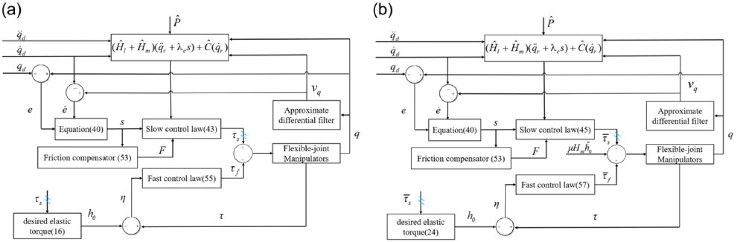
The global dynamics of the n-DOF flexible joint space manipulators described in (1), (2) and (3) are decomposed into two subsystems under the singular perturbation framework. The controllers for the slow subsystem (rigid portion) and the fast subsystem (flexible portion) are designed separately. The block diagram of the proposed adaptive controller with joint compensation is illustrated in Fig. 2.
Structure of the proposed controller for manipulators with weak (a) and strong (b) joint flexibility.

5.0 Stability Analysis
For flexible joint space manipulators, control objects can be categorised into the systems with weak joint flexibility and systems with strong joint flexibility based on their joint stiffness coefficients. Accordingly, system stability analysis is also divided into two cases of weak joint flexibility and strong joint flexibility. According to the previous section, the corrective control term  ${\tau _1}$ utilised for equivalent stiffness enhancement in flexible joint space manipulator system with strong joint flexibility is derived from the original fast controller of the manipulator with weak joint flexibility, based on the concept of integral manifold. Therefore, the stability analysis process for systems with weak and strong flexibility is similar. This section only provides the stability analysis of system with weak joint flexibility.
5.1. Slow subsystem stability analysis
For slow time scale subsystem,
 \begin{align}{V_s} = \frac{1}{2}{s^T}({H_m} + {H_l})s + \frac{1}{2}{h_1}{{\bf{\Theta }}^{\bf{T}}}{\bf{\Theta }} + \frac{1}{2}{\tilde P^T}{\bf{\Gamma }}\tilde P \gt 0\end{align}
where  ${\bf{\Theta }} = \frac{1}{{{h_1}}}{\tilde F_c} - \int_0^t {Z{{(\dot q)}^T}sd{\bf{\tau }}} $,
 ${h_1}$ is a constant and
 ${{\dot \Theta }} = - Z{(\dot q)^T}s$
Taking the derivative of  ${V_s}$ with regard to time,
 \begin{align}\nonumber{{\dot{V}}_s} &= {s^T}({H_m} + {H_l})\dot{s} + \frac{1}{2}{s^T}{{\dot{H}}_l}s + {h_1}{{\bf{\Theta }}^{\bf{T}}}{{\dot{\Theta} }} + {{\tilde{P}}^T}{\bf{\Gamma }}\dot{\tilde{P}}\\\nonumber &= {s^T}({H_m} + {H_l})(\ddot q - {{\ddot q}_r}) + \frac{1}{2}{s^T}{{\dot{H}}_l}s + {{\tilde{P}}^T}{\bf{\Gamma }}\dot{\tilde{P}} - {\rm{ }}{h_1}{{\bf{\Theta }}^{\bf{T}}}Z{(\dot{q})^T}s\\\nonumber &= {s^T}[{{\bf{\tau }}_s} - C\dot{q} - {{\bf{\tau }}_{fr}} - ({H_m} + {H_l}){{\ddot q}_r})] + \frac{1}{2}{s^T}{{\dot{H}}_l}s + {{\tilde{P}}^T}{\bf{\Gamma }}\dot{\tilde{P}} - {h_1}{{\bf{\Theta }}^{\bf{T}}}Z{(\dot{q})^T}s\\\nonumber &= {s^T}[({{\hat H}_l} + {{\hat H}_m})({{\ddot q}_r} + {\lambda _c}s) + \hat C({{\dot{q}}_r}) - {\lambda _c}({H_m} + {H_l})s - {K_s}s + F - C(s + {{\dot{q}}_r})\\ &- {{\bf{\tau }}_{fr}} - ({H_m} + {H_l}){{\ddot q}_r})] + \frac{1}{2}{s^T}{{\dot{H}}_l}s + {{\tilde{P}}^T}{\bf{\Gamma }}\dot{\tilde{P}} - {h_1}{{\bf{\Theta }}^{\bf{T}}}Z{(\dot{q})^T}s\\\nonumber &= {s^T}(Y\tilde{P} + F - {{\bf{\tau }}_{fr}} - {K_s}s - Cs) + \frac{1}{2}{s^T}{{\dot{H}}_l}s + {{\tilde{P}}^T}{\bf{\Gamma }}\dot{\tilde{P}} - {h_1}{{\bf{\Theta }}^{\bf{T}}}Z{(\dot{ q})^T}s\\\nonumber &= {s^T}Y\tilde{P} + {{\tilde{P}}^T}{\bf{\Gamma }}\dot{\tilde{P}} - {s^T}{K_s}s + {s^T}(F - {{\bf{\tau }}_{fr}}) - {h_1}{{\bf{\Theta }}^{\bf{T}}}Z{(\dot{q})^T}s\\\nonumber &= {{\tilde{P}}^T}({Y^T}s + {\bf{\Gamma }}\dot{\tilde{P}}) - {s^T}{K_s}s + {s^T}(F - {{\bf{\tau }}_{fr}}) - {h_1}{{\bf{\Theta }}^{\bf{T}}}Z{(\dot{q})^T}s\\\nonumber &= - {{\tilde{P}}^T}{\bf{\Gamma }}\tilde{P} - {s^T}{K_s}s + {s^T}[Z(\dot{q})({{\tilde{F}}_c} + {{\tilde{F}}_v} + {u_{pc}} + {u_{pv}}) + {u_u} - {F_u}(q,\dot{q})] - {h_1}(\frac{1}{{{h_1}}}{{\tilde{F}}_c} - \int_0^t {Z{{(\dot{q})}^T}sd{\bf{\tau }}} )Z{(\dot{q})^T}s\\\nonumber &= - {{\tilde{P}}^T}{\bf{\Gamma }}\tilde{P} - {s^T}{K_s}s + sZ{(\dot{q})^T}({{\tilde{F}}_v} + {u_{pv}}) + s({u_u} - {F_u}(q,\dot{q}))\end{align}
Aiming at simplify the analysis,  ${\dot V_s}$ is divided as
 ${\dot V_s} = {\dot V_1}{\rm{ + }}{\dot V_2}$, where
 ${\dot V_2}{\rm{ = }}sZ{(\dot q)^T}({\tilde F_v} + {u_{pv}})$,
 ${\dot V_1}{\rm{ = }} - {\tilde P^T}{\bf{\Gamma }}\tilde P - {s^T}{K_s}s + s({u_u} - {F_u}(q,\dot q))$.
When  $\left| {{s_i}} \right| \gt {{\bf{\varepsilon }}^i}$, combining (52) and (63) yields
 \begin{align}\nonumber{{\dot V}_1}{\rm{ = }} &- {{\tilde P}^T}{\bf{\Gamma }}\tilde P - {s^T}{K_s}s + s( {-} {{\bf{\rho }}_f}\frac{s}{{\left| s \right|}} - {F_u}(q,\dot q))\\\nonumber = &- {{\tilde P}^T}{\bf{\Gamma }}\tilde P - {s^T}{K_s}s - {{\bf{\rho }}_f}\left| s \right| - {F_u}(q,\dot q)s\\ = &- {{\tilde P}^T}{\bf{\Gamma }}\tilde P - {s^T}{K_s}s - \left| s \right|({{\bf{\rho }}_f} - {F_u}(q,\dot q)\frac{s}{{\left| s \right|}})\\ \lt &- {{\tilde P}^T}{\bf{\Gamma }}\tilde P - {s^T}{K_s}s\nonumber\end{align}
When  $\left| {{s_i}} \right| \le {{\bf{\varepsilon }}^i}$
 \begin{align}\nonumber{{\dot V}_1}{\rm{ = }} &- {{\tilde P}^T}{\bf{\Gamma }}\tilde P - {s^T}{K_s}s + s( {-} {{\bf{\rho }}_f}\frac{s}{{\bf{\varepsilon }}} - {F_u}(q,\dot q))\\ = &- {{\tilde P}^T}{\bf{\Gamma }}\tilde P - {s^T}{K_s}s - \frac{{{{\bf{\rho }}_f}}}{{\bf{\varepsilon }}}{s^2} - {F_u}(q,\dot q)s\\ \le &- {{\tilde P}^T}{\bf{\Gamma }}\tilde P - {s^T}{K_s}s - \frac{{{{\bf{\rho }}_f}}}{{\bf{\varepsilon }}}{s^2} + {{\bf{\rho }}_f}\left| s \right|\nonumber\end{align}
The term  $ - ({{\bf{\rho }}_f}/{\bf{\varepsilon }}){s^2} + {{\bf{\rho }}_f}\left| s \right|$ reaches its maximum value
 $ - {{\bf{\rho }}_f}{\bf{\varepsilon }}/4$ when
 $\left| s \right| = {\bf{\varepsilon }}/4$. It is evident that
 \begin{align}{\dot V_1} \le - {\tilde P^T}{\bf{\Gamma }}\tilde P - {s^T}{K_s}s + \frac{{{{\bf{\rho }}_f}{\bf{\varepsilon }}}}{4}\end{align}
Since
 \begin{align}sZ{(\dot q)^T}({\tilde F_v} + {u_{pv}}) = \sum\limits_{n = 1}^4 {{s_i}Z{{(\dot q)}^T}} ({\tilde F_{vn}} + {u_{pvn}}) = \sum\limits_{n = 1}^4 {{\zeta _n}({{\tilde F}_{vn}} + {u_{pvn}})} \end{align}
According to (51) if  $\left| {\zeta _n^i} \right| \gt {\bf{\varepsilon }}_{pvn}^i$, for n = 1,2,3,4
 \begin{align}{\zeta _n}({\tilde F_{vn}} + {u_{pvn}}) = {\zeta _n}({\tilde F_{vn}} - {{\bf{\delta }}_{vn}}\frac{{{\zeta _n}}}{{\left| {{\zeta _n}} \right|}}) \lt 0\end{align}
If  $\left| {\zeta _n^i} \right| \le {\bf{\varepsilon }}_{pvn}^i$
 \begin{align}{\zeta _n}({\tilde F_{vn}} + {u_{pvn}}) = {\zeta _n}({\tilde F_{vn}} - {{\bf{\delta }}_{vn}}\frac{{{\zeta _n}}}{{{{\bf{\varepsilon }}_{pvn}}}}) \le {\zeta _n}({{\bf{\delta }}_{vn}}\frac{{{\zeta _n}}}{{\left| {{\zeta _n}} \right|}} - {{\bf{\delta }}_{vn}}\frac{{{\zeta _n}}}{{{{\bf{\varepsilon }}_{pvn}}}})\end{align}
(69) reaches its maximum value  ${{\bf{\rho }}_f}{\bf{\varepsilon }}/4$ when
 $\left| {{\zeta _n}} \right| = {{\bf{\varepsilon }}_{pvn}}/2$. It can be observed that
 \begin{align}{\dot V_2} \le \sum\limits_{n = 1}^4 {{{\bf{\delta }}_{vn}}{{\bf{\varepsilon }}_{pvn}}/4} \end{align}
Combining the results in (64), (66), (68) and (70), the following inequality can be obtained:
 \begin{align}{\dot V_s} \le - {\tilde P^T}{\bf{\Gamma }}\tilde P - {s^T}{K_s}s + \frac{{{{\bf{\rho }}_f}{\bf{\varepsilon }}}}{4} + \sum\limits_{n = 1}^4 {{{\bf{\delta }}_{vn}}{{\bf{\varepsilon }}_{pvn}}/4} \end{align}
Inequality (71) leads to the conclusion that a Lyapunov function can be located if only
 \begin{align}\left| s \right| \ge \frac{1}{2}\sqrt {\frac{{{{\bf{\rho }}_f}{\bf{\varepsilon }} + \sum\limits_{n = 1}^4 {{{\bf{\delta }}_{vn}}{{\bf{\varepsilon }}_{pvn}}} }}{{{K_s}}}} \end{align}
On the other hand, when
 \begin{align}\left| s \right| \lt \frac{1}{2}\sqrt {\frac{{{{\bf{\rho }}_f}{\bf{\varepsilon }} + \sum\limits_{n = 1}^4 {{{\bf{\delta }}_{vn}}{{\bf{\varepsilon }}_{pvn}}} }}{{{K_s}}}} \end{align}
Based on the conclusion presented by Slotine and Li [Reference Qiao, Qu and Deng29],  $\dot e$ and
 ${\dot e_i}$ are also bounded if
 $s$ is bounded.
5.2 Fast subsystem stability analysis
For the fast time scale subsystem,
 \begin{align}{V_f} = \frac{1}{2}{{\mu }}({{{\dot \eta }}^T}{{\dot \eta }} + {{\bf{\eta }}^T}{{\dot \eta }}{\rm{ + }}{{\bf{\eta }}^T}{\bf{\eta }})\end{align}
Defining  ${\bf{\Omega }}\,{\rm{ = }}\,{({{\bf{\eta }}^T},{{{\dot \eta }}^T})^T}$, V are rewritten as
 \begin{align}{V_f} = \frac{1}{2}{{\mu }}{{\bf{\Omega }}^T}H{\bf{\Omega }} \ge \frac{1}{2}{{\mu }}{{\bf{\lambda }}_{\min }}\left\{ H \right\}{\left\| {\bf{\Omega }} \right\|^2} \ge 0\end{align}
where  $H = \left( {\begin{array}{{c}}\,\,\,1\quad{1/2}\\\!\!\!{1/2}\,\,\,\,\,\,1\end{array}} \right)$.
Taking the derivative of the Lyapunov function candidate  ${V_f}$ with regard to the fast scaled time
 ${\bf{\delta = t/\mu }}$, and substituting the elastic torque error equation
 \begin{align}{{\dot V}_f} &= {{{{\dot \eta }}}^T}{{\ddot \eta }} + \frac{1}{2}{{{{\dot \eta }}}^T}{{\dot \eta }} + \frac{1}{2}{{\bf{\eta }}^T}{{\ddot \eta }}{\rm{ + }}{{\bf{\eta }}^T}{{\dot \eta }}\nonumber\\ &= {{{{\dot \eta }}}^T}( {-} {a_1}{\bf{\eta }} - {a_2}{{\dot \eta }}) + \frac{1}{2}{{{{\dot \eta }}}^T}{{\dot \eta }} + \frac{1}{2}{{\bf{\eta }}^T}( {-} {a_1}{\bf{\eta }} - {a_2}{{\dot \eta }}) + {{\bf{\eta }}^T}{{\dot \eta }}\\ &= - {{{{\dot \eta }}}^T}{a_2}{{\dot \eta }} + \frac{1}{2}{{{{\dot \eta }}}^T}{{\dot \eta }} - {{{{\dot \eta }}}^T}{a_1}{\bf{\eta }} - \frac{1}{2}{{\bf{\eta }}^T}{a_2}{{\dot \eta }} + {{\bf{\eta }}^T}{{\dot \eta }} - \frac{1}{2}{{\bf{\eta }}^T}{a_1}{\bf{\eta }}\nonumber\end{align}
The following inequalities can be established determined by Rayleigh–Ritz inequality [Reference Khosravi and Taghirad20],
 \begin{align}\begin{array}{c} - {{{{\dot \eta }}}^T}{a_2}{{\dot \eta }} \le - {{\bf{\lambda }}_{\min }}({a_2}){\left\| {{{\dot \eta }}} \right\|^2}\\[6pt]\frac{1}{2}{{{{\dot \eta }}}^T}{{\dot \eta }} \le \frac{1}{2}{\left\| {{{\dot \eta }}} \right\|^2}\\[6pt] - {{{{\dot \eta }}}^T}{a_1}{\bf{\eta }} \le - {{\bf{\sigma }}_{\min }}({a_1})\left\| {{{\dot \eta }}} \right\|\left\| {\bf{\eta }} \right\|\\[6pt] - \frac{1}{2}{{\bf{\eta }}^T}{a_2}{{\dot \eta }} \le - \frac{1}{2}{{\bf{\sigma }}_{\min }}({a_2})\left\| {\bf{\eta }} \right\|\left\| {{{\dot \eta }}} \right\|\\{{\bf{\eta }}^T}{{\dot \eta }} \le \left\| {\bf{\eta }} \right\|\left\| {{{\dot \eta }}} \right\|\\[3pt] - \frac{1}{2}{{\bf{\eta }}^T}{a_1}{\bf{\eta }} \le - {{\bf{\lambda }}_{\min }}({a_1}){\left\| {\bf{\eta }} \right\|^2}\end{array}\end{align}
where  ${{\bf{\sigma }}_{\min }}(\!\cdot\!)$ and
 ${{\bf{\lambda }}_{\min }}(\!\cdot\!)$ denote the matrix’ the minimum singular and minimum eigenvalue value, respectively.
Equation (76) can be expressed as follows by sequentially applying the aforementioned inequalities:
 \begin{align}{\dot V_f} \le - {T^T}QT\end{align}
where
 \begin{align*}T = \left( {\begin{array}{*{20}{c}}{\left\| {{{\dot \eta }}} \right\|}\\{\left\| {\bf{\eta }} \right\|}\end{array}} \right),Q = \left(\quad {\begin{array}{*{20}{c}}{{{\bf{\lambda }}_{\min }}({a_2}) - \frac{1}{2}} {}\quad\,\,\,\,\,{\frac{{2{{\bf{\sigma }}_{\min }}({a_1}) + {{\bf{\sigma }}_{\min }}({a_2}) - 2}}{4}}\\[6pt]\!\!\!\!\!\!\!\!\!\!\!\!\!\!\!\!\!{\frac{{2{{\bf{\sigma }}_{\min }}({a_1}) + {{\bf{\sigma }}_{\min }}({a_2}) - 2}}{4}}\,\,\,\,\,\,\,\,\,\,\,\quad {}{{{\bf{\lambda }}_{\min }}({a_1})}\end{array}} \right)\end{align*}
In order to guarantee that  ${\dot V_f}$ is negative-definite, Q must satisfy the following inequalities so as to be a positive-definite matrix:
 \begin{align}{{\bf{\lambda }}_{\min }}({a_2}) \gt \frac{1}{2},({{\bf{\lambda }}_{\min }}({a_2}) - \frac{1}{2}){{\bf{\lambda }}_{\min }}({a_1}) - {\bigg(\frac{{2{{\bf{\sigma }}_{\min }}({a_1}) + {{\bf{\sigma }}_{\min }}({a_2}) - 2}}{4}\bigg)^2} \gt 0\end{align}
Therefore, if the above condition (79) holds,  ${V_f}$ is positive-definite,
 ${\dot V_f}$ is negative-definite, the asymptotic stability of fast subsystem can be demonstrated.
5.3 The entire system stability analysis
For the entire system, the Lyapunov function candidate is considered as follows: [Reference Khosravi and Taghirad20]
 \begin{align}V = {V_s} + {V_f}\end{align}
where Vs represents the Lyapunov function candidate for the slow time scale subsystem shown in equation (17) and  ${V_f}$ represents that for the fast time scale subsystem shown in equation (21), and both
 ${c_1}$ and
 ${c_2}$ are positive constants. It is evident from the previous proof that
 $V = {V_s} + {V_f}$ is positive-definite.
Obviously
 \begin{align}\dot V = {\dot V_s} + {\dot V_f}\end{align}
The stability of the first part of equation is proven using a similar method to that in Section 5.1. It is important to note a key difference: equation (10) is used to replace equation (17) and is then substituted into  ${\dot V_s}$, because of the representation of the entire system by equations (10) and (11). The stability proof of the fast time scale subsystem employs the same as approach that described in the previous part. Aa a result, it is determined that
 $\dot V$ is negative definite, leading the conclusion that the entire composite system is asymptotically stable.
6.0 Simulation Results
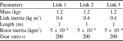
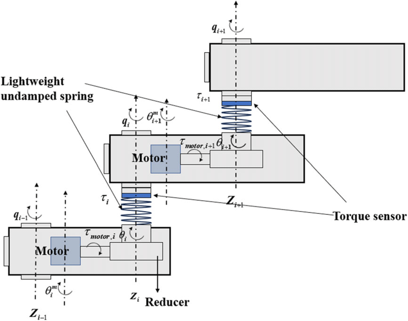
This section aims to demonstrate the effective performance of the proposed controller by conducting simulations on a three-link flexible-joint space manipulator (Table 1) with different joint stiffnesses and comparing its control effect with that of the traditional adaptive controller (TAC) [Reference Liu and Huang30]. The simulation model is shown in Fig. 3.
Manipulator’s parameters for simulation

Simulation model of space manipulator.

The following is the expressions for  ${H_l}(q)$,
 $C(q,\dot q)$ with respect to the elements of the space manipulator parameters vector
 $P$:
 \begin{align} & {H_l}(q) = \left[ \begin{array}{l@{\quad}l@{\quad}l} {{H_l}_{11}} & {} {{H_l}_{12}} & {}{{H_l}_{13}} \\ {{H_l}_{21}} & {{H_l}_{22}} & {}{{H_l}_{23}} \\ {{H_l}_{31}} & {{H_l}_{32}} & {}{{H_l}_{33}} \end{array} \right],C(q,\dot q) = \left[ \begin{array}{l@{\quad}l@{\quad}l} {{C_{11}}} & {}{{C_{12}}} & {}{{C_{13}}} \\ {{C_{21}}} & {{C_{22}}} & {}{{C_{23}}} \\ {{C_{31}}} & {{C_{32}}} & {}{{C_{33}}} \end{array} \right],J = diag\left\{ {0.2,0.2,0.2} \right\} \nonumber\\ \nonumber
&{H_l}_{11} = {p_1} + {p_4} + {p_5} + {p_9}\cos {q_2} + 2{p_7}\cos {q_2} + {p_6}\cos ({q_2} + {q_3}) + {p_8}\cos {q_3} \\ \nonumber
&{H_l}_{12} = {H_l}_{21} = {p_2} + {p_5} + 0.5{p_9}\cos {q_2} + {p_8}\cos {q_3} + {p_7}\cos {q_2} + 0.5{p_6}\cos ({q_2} + {q_3}) \\ \nonumber
&{H_l}_{13} = {H_l}_{31} = {p_3} + 0.5{p_8}\cos {q_3} + 0.5{p_6}\cos ({q_2} + {q_3}) \\ \nonumber
&{H_l}_{22} = {p_2} + {p_5} + {p_8}\cos {q_3} \\ \nonumber
&{H_l}_{23} = {H_l}_{32} = {p_3} + 0.5{p_8}\cos {q_3} \\ \nonumber
&{H_l}_{33} = {p_3} \\ \nonumber
&{C_{11}} = - 0.5{p_9}{{\dot q}_2}\sin ({q_2}) - 0.5{p_6}{{\dot q}_3}\sin ({q_2} + {q_3}) - 0.5{p_6}{{\dot q}_2}\sin ({q_2} + {q_3}) - {p_7}{{\dot q}_2}\sin ({q_2}) - 0.5{p_8}{{\dot q}_3}\sin {q_3} \\ \nonumber
&{C_{12}} = - 0.5{p_9}({{\dot q}_1} + {{\dot q}_2})\sin ({q_2}) - 0.5{p_6}({{\dot q}_1} + {{\dot q}_2} + {{\dot q}_3})\sin ({q_2} + {q_3}) - {p_7}({{\dot q}_1} + {{\dot q}_2})\sin ({q_2}) \\ \nonumber
&{C_{13}} = - 0.5{p_8}{{\dot q}_2}\sin {q_3} - 0.5{p_6}({{\dot q}_1} + {{\dot q}_2} + {{\dot q}_3})\sin ({q_2} + {q_3}) - 0.5{p_8}({{\dot q}_1} + {{\dot q}_2} + {{\dot q}_3})\sin {q_3} \\ \nonumber
&{C_{21}} = 0.5{p_9}{{\dot q}_1}\sin {q_2} + 0.5{p_6}{{\dot q}_1}\sin ({q_2} + {q_3}) + {p_7}{{\dot q}_1}\sin ({q_2}) \\ \nonumber
&{C_{22}} = - 0.5{p_8}{{\dot q}_3}\sin {q_3} \\ \nonumber
& {C_{23}} = - 0.5{p_8}{{\dot q}_2}\sin {q_3} - 0.5{p_8}{{\dot q}_3}\sin {q_3} - {p_8}{{\dot q}_1}\sin {q_3} \\ \nonumber
& {C_{31}} = {p_8}{{\dot q}_1}\sin {q_3} + 0.5{p_8}{{\dot q}_2}\sin {q_3} \\ \nonumber
& {C_{33}} = 0 \\ \nonumber
& P = (\begin{array}{l@{\quad}l@{\quad}l@{\quad}l@{\quad}l@{\quad}l@{\quad}l@{\quad}l@{\quad}l} {{p_1}} & {}{{p_2}} & {}{{p_3}} & {} {{p_4}} & {}{{p_5}} & {}{{p_6}} & {}{{p_7}} & {}{{p_8}} & {}{{p_9}})^{T} \end{array}\end{align}
About the friction compensation F, the parameters for the simulation are set as:
 \begin{align}\begin{array}{l}{B_i} = 2.5 + 0.7\sin\!(10{q_i})Nm{\rm{ }}s/rad\\\nonumber{F_{ci}} = 4.5 + 0.5\sin\!(10{q_i})Nm\\\nonumber{F_{si}} = 5 + 0.7\sin\!(10{q_i})Nm{\rm{ }}\\\nonumber{F_{{\bf{\tau }}i}} = 100 + 20\cos\!(10{q_i}){s^2}/ra{d^2}\end{array}\end{align}
The following are the uncertainty boundaries and associated parameters:
 \begin{align}{h_1} = {h_2} = {h_3} = 1,{\bf{\varepsilon }}_{pvn}^i = 0.01,{{\bf{\varepsilon }}^i} = 0.1,{{\bf{\rho }}_{fi}} = 0.5,{}^i{{\bf{\delta }}_{v1}} = {}^i{{\bf{\delta }}_{v3}} = 0.7,{}^i{{\bf{\delta }}_{v2}} = 0.5,{}^i{{\bf{\delta }}_{v4}} = 20\nonumber\end{align}
The nominal friction parameters of the proposed friction model are as follows:
 \begin{align}{\hat B_i} = 1.8Nm{\rm{ }}s/rad,{\hat F_{ci}} = 3.6Nm,{\hat F_{si}} = 4.0Nm{\rm{,}}\,{\hat F_{{\bf{\tau }}i}} = 80{s^2}/ra{d^2}\nonumber\end{align}
Position-dependent friction and other friction modeling errors  ${F_{ui}}({q_i},{\dot q_i})$ in friction models described as
 $0.5\sin (3q)$.
For simplicity, the same friction model and parameters were selected for all joints. The following is the desired trajectories for three joints:
 \begin{align}\begin{array}{l}{q_{d1}} = 1/(2\pi )\sin (2\pi t + \pi /2)rad\\\nonumber{q_{d2}} = 1/(2\pi )\sin (2\pi t + \pi /2)rad\\\nonumber{q_{d3}} = 1/(2\pi )\sin (2\pi t + \pi /2)rad\end{array}\end{align}
For a three-link flexible-joint space manipulator (Table 1) with weak joint flexibility, namely K=10,000, simulations were conducted to compare the provided novel adaptive controller (NAC) with the TAC, verifying the effectiveness of the proposed control strategy.
The control law of NAC is presented by equations (43), (44), (53) and (55). The control law of TAC is given by equation (82):
 \begin{align}\begin{array}{l}{{\bf{\tau }}_s}' = ({{\hat{H}}_l} + {{\hat{H}}_m}){{\ddot q}_r} + \hat{C}{{\dot q}_r} - {K_s}s + F,\\\dot{\hat{P}}' = - {{\bf{\Gamma }}^{ - 1}}{Y^T}(q,\dot q,{{\dot q}_r},{{\ddot q}_r})s,\\{{\bf{\tau }}_f}' = {A_1}{\bf{\eta }} + {A_2}{{\dot \eta }}\end{array}\end{align}
where  ${\tau _s}'$ and
 ${\tau _f}'$ act on the slow and fast subsystem, respectively.
After trials and errors, the same parameters for both controllers (TAC, NAC) take the following values:
 \begin{align}\begin{array}{c}{\bf{\Gamma }} = diag\{ 100,100,100,100,100,100,100,100,100\} \\\nonumber{K_s} = diag\{ 600,600,600\} ,{\bf{\Lambda }} = diag\{ 80,80,80\} \\\nonumber{A_1} = diag\{ 1.5,1.5,1.5\} ,{A_2} = diag\{ 0.03,0.03,0.03\} \end{array}\end{align}
The standard criteria proposed in [Reference Liu and Huang30] were adopted to evaluate the control performance. This represents the average performance with regard to tracking errors.
 \begin{align}RMS({e_i}) = \sqrt {{{\int_0^T {\left| {{e_i}} \right|} }^2}dt/T} ,i = 1,2,3\end{align}
 \begin{align}RMS({\bf{e}}) = \sqrt {{{\int_0^T {\left\| {\bf{e}} \right\|} }^2}dt/T}\\\nonumber\end{align}
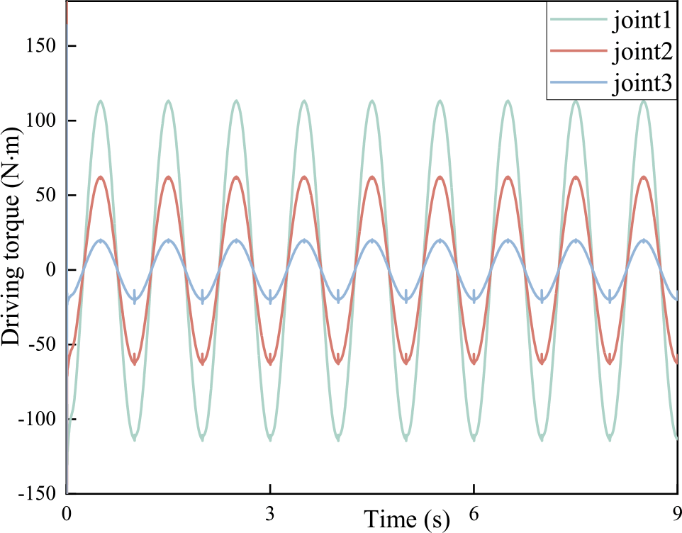
Figure 7 illustrates the driving torque of all joints utilising the adaptive control method (NAC) proposed in this paper.
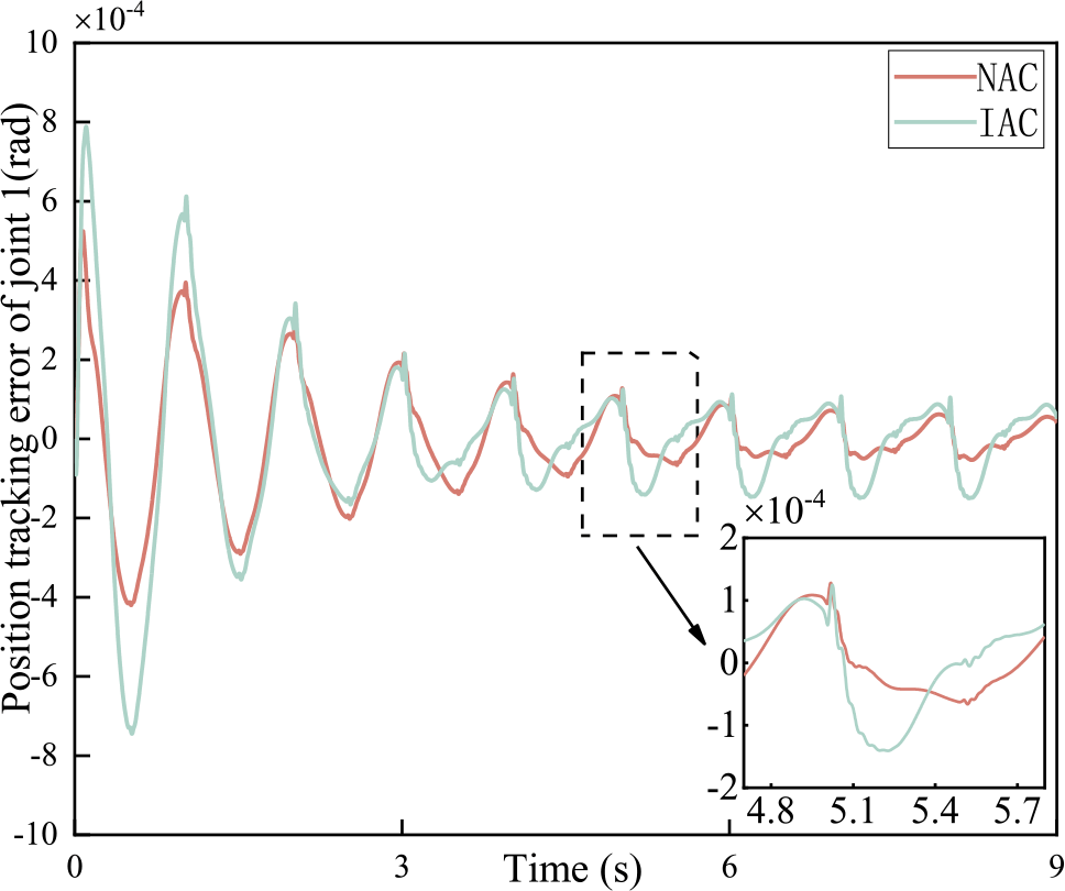
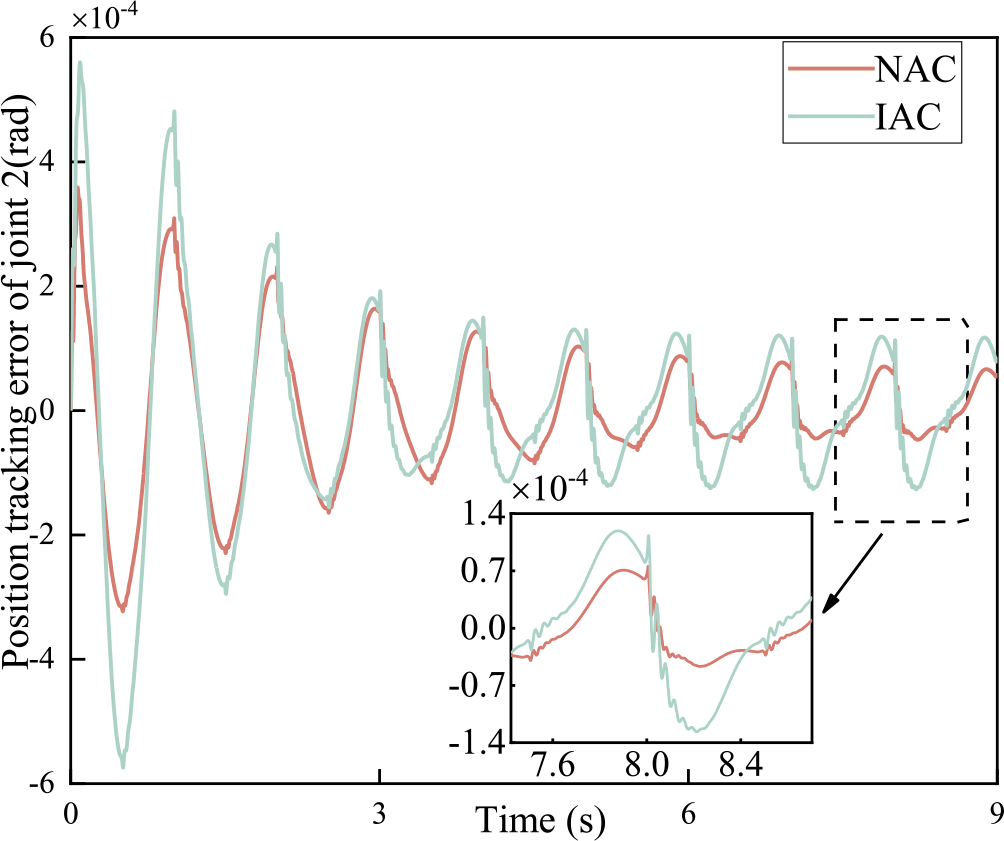
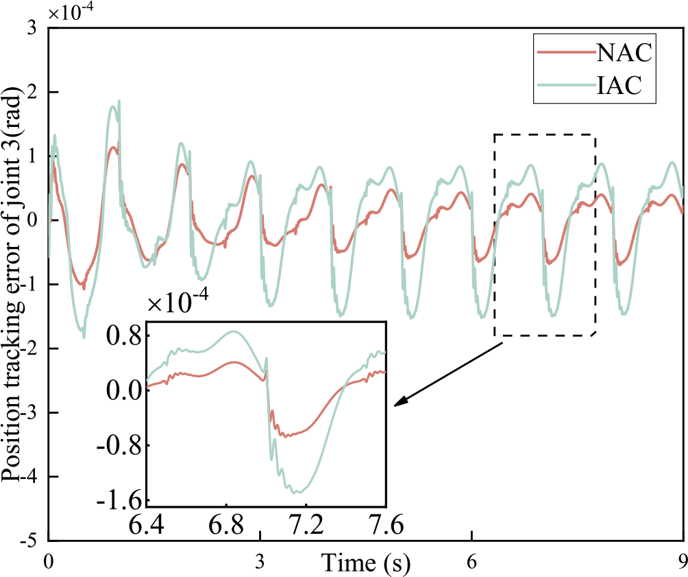
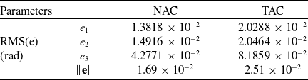
Simultaneously, from the position tracking error curves in Figs 4, 5 and 6, it is evident that the presented adaptive control strategy yields smaller position errors than the traditional that (TAC). The reason for this is that the proposed control approach employs an enhanced linear parameterisation formulation by (41) that improves the estimation accuracy of adaptive parameters. As demonstrated in Table 2, the RMS(e) in the proposed approach (NAC) decreases by 31.8% at the first joint, 27.1% at the second joint, 8.7% at the third joint and 28.1% on the overall compared with these of the controller (TAC), respectively. Furthermore, an approximate differential filter is used to estimate the velocity signal of the links, avoiding noise contamination from measuring the velocity signal directly and improving the robustness of the control system. Typically, the higher the applied torque, the lesser the impact of friction on the variation of joint angle. As can be observed from the Figs 4–6, the effect of friction on the variation of joint angles is more pronounced in joint 3 as compared to joints 1 and 2. However, the jitter in the error curve due to friction is slight, indicating that it is well suppressed by the friction compensator. Simulation results demonstrate that the adaptive controller provided in the paper can well suppress the effects of joint vibration and joint friction on the accurate movements of manipulators.
Tracking error of joint 1(K = 10,000).

Tracking error of joint 2(K = 10,000).

Tracking error of joint 3(K = 10,000).

Performance comparison (K = 10,000)

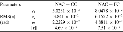
Performance comparison (K = 2,000)

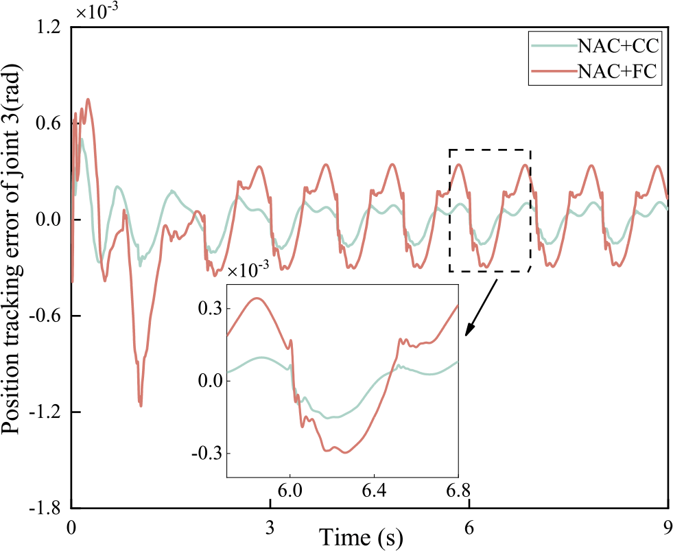
Previous simulation results indicate that the adaptive controller proposed in the paper achieves better trajectory tracking when system stiffness is high (i.e. system with weak joint flexibility). For a manipulator system with strong joint flexibility, to verify the effectiveness and superiority of the corrective control scheme (CC) proposed in Section 3.3, comparative simulations are conducted on the provided NAC with the corrected control term in this paper and the provided NAC with the flexibility compensator (FC) in the literature [Reference Yu and Chen31].
The following is a description of the flexibility compensator in the literature [Reference Yu and Chen31].
 \begin{align}{\tau _1}' = {K_t}\tau ,{\tau _m}' = {K_a}({\tau _s}' + {\tau _f}') + {\tau _1}'\end{align}
where  ${\tau _m}'$ represents the composite control input torque,
 ${\tau _1}'$ represents the flexibility compensation section,
 ${K_t}$ and
 ${K_a}$ are fixed-parameter matrices. The two matrices satisfy the relationship:
 ${K_a} = I + {K_t}$.
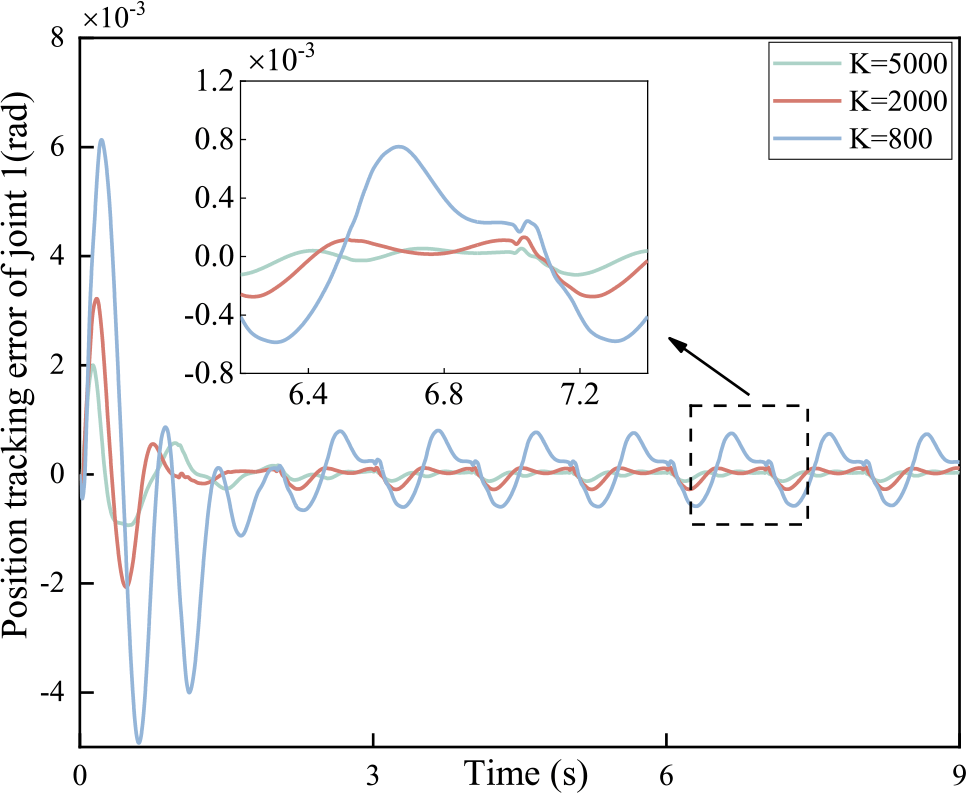
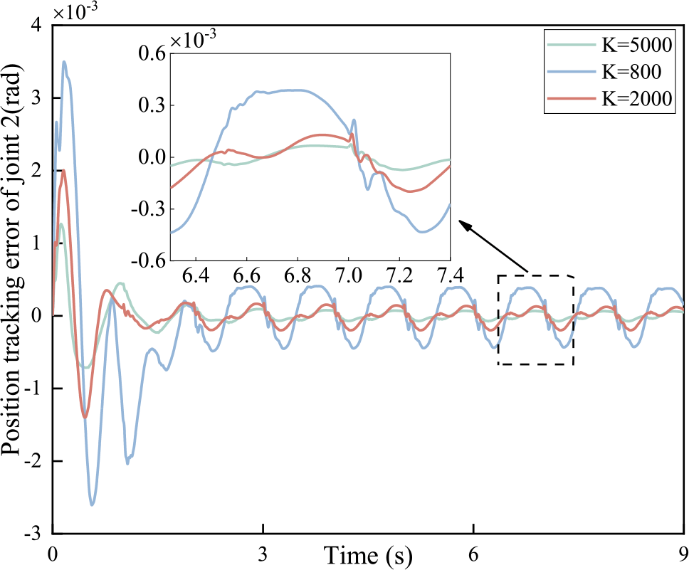
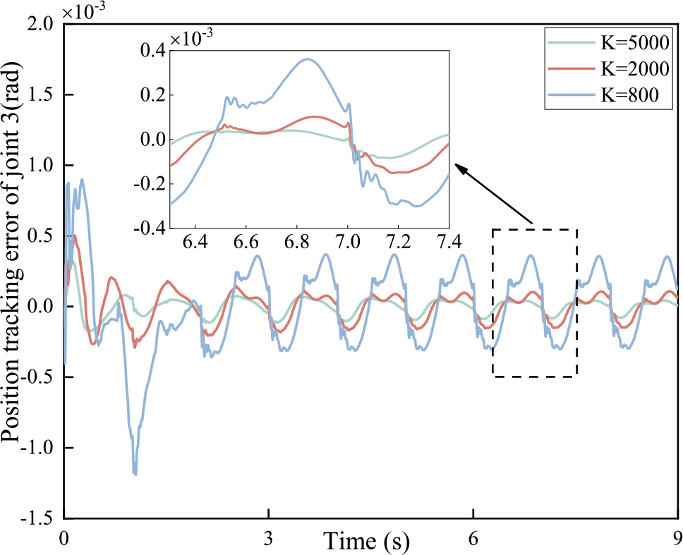
Note that, to validate the effectiveness of the provided NAC + CC, simulations are conducted on the manipulator (Table 1) with different joint stiffness coefficient (namely K=5,000, 2,000 and 800, respectively). After trials and errors, the parameters take the following values:
 \begin{align}\begin{array}{c}{\bf{\Gamma }} = diag\{ 100,100,100,100,100,100,100,100,100\} \\\nonumber{K_s} = diag\{ 300,300,300\} ,{\bf{\Lambda }} = diag\{ 80,80,80\} \\\nonumber{{\bar A}_1} = diag\{ 8,8,8\} ,{{\bar A}_2} = diag\{ 0.09,0.09,0.09\} \end{array}\end{align}
As shown in Figs 8, 9 and 10, it is clearly noticed that the trajectory tracking error curves of the three joints almost coincide when the stiffness coefficients K = 5,000 and K = 2,000, and the absolute value of the error in the steady state remains at the order of 10-4. The results indicate that the calibratable control law can effectively compensate for strong flexibility in the system, and it has excellent adaptability to the systems with different strong flexibility (under different stiffness coefficients, the system controller does not need to change the simulation parameters). However, when the stiffness coefficient K = 800, the trajectory tracking error significantly increases in the steady state compared to the first two cases, and the regulation time also increases. This indicates that when the joint flexibility of the system exceeds a certain limit, the proposed correctable control law for flexibility compensation is less effective for enhancing the equivalent system’s stiffness. However, it still manages to maintain a good error steady state.
Driving torque of three joints (NAC).

Tracking error of joint 1.

Tracking error of joint 2.

Tracking error of joint 3.

Observe that, for the three-link flexible-joint space manipulator (Table 1) with strong joint flexibility (namely K = 2,000), simulations are conducted to compare the provided novel adaptive controller with the corrected control term (CC) in this paper and the provided novel adaptive controller with the FC. The parameters for controllers take the following values:
 \begin{align}\begin{array}{c}{\bf{\Gamma }} = diag\{ 100,100,100,100,100,100,100,100,100\} \\\nonumber{K_s} = diag\{ 300,300,300\} ,{\bf{\Lambda }} = diag\{ 80,80,80\} \\\nonumber{{\bar A}_1} = diag\{ 8,8,8\} ,{{\bar A}_2} = diag\{ 0.09,0.09,0.09\} \\\nonumber{K_t} = diag\{ 120,120,120\} ,{K_a} = diag\{ 121,121,121\} \end{array}\end{align}
Observing Figs 11, 12 and 13, it is evident that both the corrective control law and the flexibility compensator effectively enhance stiffness in the flexible joint space manipulator system with strong joint flexibility, successfully overcoming the vibrations generated at the flexible joints. However, the choice of tuning parameters for the latter is constrained by factors such as unmodeled dynamics, sensor noise and signal sampling frequency, preventing the indefinite scaling up of equivalent stiffness [Reference Liu, Jin and Liu33]. Furthermore, in terms of regulation time and steady-state error value, the former performs slightly better.
Tracking error of joint 1(K = 2,000).

Tracking error of joint 2(K = 2,000).

Tracking error of joint 3(K = 2,000).

7.0 Conclusions
This paper provided a novel adaptive control approach according to singularly perturbed decoupling and integral manifold concept for flexible-joint space manipulators considering parametric uncertainties and joints friction. The control scheme includes a decomposition-based friction compensator, a modified compensation term to enhance system stiffness, and a composite adaptive controller to mitigate joint flexibility. The decomposition-based friction compensation scheme aims to deal with various kinds of model uncertainty in an appropriate way. An adaptive compensator addresses the unknown but constant portion of the variable parametric friction model uncertainty, while a robust compensator manages the variable yet bounded portion. It is emphasised by an enhanced parameter linearisation formulation and an approximate differential filter invoked in the proposed controller. Approximate differential filters are utilised to estimate the joint velocities of the links and the differential terms of joint elastic torques, which reduces noise disturbances and improves the robustness of the control system. Moreover, a modified compensation law is proposed to enhance system stiffness, addressing the limitations of the traditional singular perturbation method, which is only suitable for space manipulators with weak joint flexibility. In addition, the asymptotic stability of the system is proved based on Lyapunov’s theory. Finally, simulations presented on a three-degree-of-freedom manipulator are illustrated to examine the performance of the provided control strategy and comparisons with the TAC to verify the superiorities of the provided controller.
8.0 Future Work
While the proposed adaptive control approach demonstrates promising performance in simulation environments, several avenues remain open for further exploration to advance its theoretical foundations and practical applicability:
Experimental Validation on Physical Platforms: Implementing the controller on a ground-based space manipulator testbed to evaluate its robustness under real-world disturbances. This will bridge the gap between theoretical design and practical deployment.
Multi-Objective Optimisation: Integrating trajectory planning with the adaptive controller to jointly optimise energy efficiency, vibration suppression and tracking accuracy. Techniques such as dynamic programming or reinforcement learning could be explored to address this coupled optimisation problem.
Data-Driven Friction Compensation: Enhancing the friction compensator by incorporating neural networks or Gaussian processes to model unmeasured nonlinearities. Hybrid models combining physics-based and data-driven approaches may further improve compensation accuracy.
Declaration of Competing Interest
The authors declare that they have no known competing financial interests or personal relationships that could have appeared to influence the work reported in this paper.