2.1 Field equations

Ice is treated as an incompressible viscous fluid, Its mechanical properties may depend on other fields of physical quantities, such as temperature and stress. The geometry of the ice mass is defined by the upper free surface S = S(x,y) and the basal surface B = B(x,y) in Cartesian coordinates (x,y,z) with the z axis pointing opposite to the direction of gravity. The equation for mass continuity then becomes

where u, v and w are the velocity components in the x,y and z directions, respectively, and for linear momentum

where ρ is the density of ice. g is the acceleration of gravity and τ_xx, τ_yy, τ_zz, τ_xz, τ_yz and τ_xy are the components of the symmetric Cauchy stress tensor τ_ij. Glacier ice is generally treated as a non-Newtonian fluid with a stress strain-rate relation of the form

where σ_ij = τ_ij − (1/3)τ_kkδ_ij is the deviatoric stress tensor and σ_xx. and σ_yy are the normal deviatoric stress components. Due to the incompressiblity condition in Equation (2.1), an additional equation relating ∂w/∂z to σ_zz is redundant and can be omitted. The term AF(·) represents a flow law. In this study, a flow law of the form (Reference NyeNye. 1953; Reference GlenGlen. 1958; Reference MeierMeier. 1958)

is used, where T is the effective stress (second invariant of the deviatoric stress tensor), µ is the viscosity and µ₀ = 1/ΑΤ₀ ⁿ⁻¹ is the viscosity in the limit of vanishing stress. The rate factor A is usually assumed to depend exclusively on temperature. The absence of pressure-dependence, e.g. considered in Reference Weertman, Whalley, Jones and GoldWeertman (1973), is crucial for the applicability of the algorithm introduced below. Substituting Equations (2.5) and (2.6) into Equation (2.1) yields

which is easier to handle than Equation (2.1) in the numerical integration scheme described in sections 3.1 and 3.2. For the upper free surface S = S(x,y), the boundary conditions for stress are

where

are the components of the normal Vector n pointing outward from the ice and P is the pressure on the outer side of the surface. Note, in this simple form, the vector n is not a unit vector. In the case of a grounded ice sheet with no basal melt or freezing and no isostatic uplift, basal motion is to a good approximation parallel to the bed

in the case of sliding, and u=v=w = 0 in the case of non-sliding conditions.

2.2 Scale analysis

To arrive at a consistent simplified set of equations, we need to estimate the order of magnitude of the various terms in the equations. To this end. we introduce a scaling for spatial variables x, y, z, S and B.,

the velocity components u, v, and w,

the stress components τ_ij, σ_kk and the pressure P,

and for the rate factor A

where {L} and {H} denote the characteristic horizontal and vertical extents of the ice sheet, respectively, A₀ is a typical rate factor, and

and à are the corresponding dimensionless scaled variables of order unity. This specific scaling only applies if we assume ice behaves according to the generalized (Glen flow law Equation (2.10)). Since the extent of an ice sheet is much larger than its thickness, the aspect ratio ϵ = {H}/{L} ≪ 1 is used as scaling parameter. We define the first-order approximation by deleting terms of order ϵ² but retaining terms of order 1 and ϵ. Although the first-order approximation can also be considered as a shallow-ice approximation (Reference Dahl-JensenDahl-Jensen. 1989), the term “shallow-ice approximation” will be used only for the “zeroth”-order approximation in the rest of this paper; for simplicity, the first-order shallow-ice approximation will be referred to as “first-order” approximation.

Scaling the continuity Equation (2.11), the stress Equations (2.2)–(2,4) and the constitutive Equations (2.5)–(2.9) yield

and the surface-boundary conditions for stress in Equations (2.12)–(2.14) in the scaled form are

To eliminate the normal Cauchy stresses in Equations (2.22)–(2.24), we follow the usual procedure (see e.g. Reference Hetterich, Van der Veen and OerlemansHerterich, 1987) by deleting terms of order O(ϵ²) in Equation (2.24) and integrating the truncated equations from

to the surface, and applying the result in Equations (2.22) and (2.23). Integration yields

Using Equation (2.32) and the relation between Cauchy stresses and deviatoric stresses in the form

in Equation (2.33) and dropping terms of order O(ϵ²) yields

We differentiate Equations (2.35) and (2.36) and substitute the result in Equations (2.22) and (2,23), respectively, to obtain

Similarily, eliminating

, and in the boundary conditions in Equations (2.30)–(2.32) and dropping terms of order ϵ² gives the corresponding first-order boundary conditions (Reference Morland and ShoemakerMorland and Shoemaker. 1982; Reference MorlandMorland, 1984)

Finally, we get eight independent Equations (2.37), (2.38), (2.21) and (2.25)–(2.29) for the eight unknown field variables

and . This set of eight equations only Constitutes a well-posed problem for the eight unknown field variables, if the rate factor à is independent of pressure (i.e. of normal Cauchy stresses).

3.1 Coordinate transformation

The numerical scheme used for integrating the above set of first-order equations was developed by Reference MullerMuller (1991) for the two-dimensional plane-strain approximation, and is extended here for the three-dimensional case. We apply a coordinate transformation (Reference PhillipsPhillips, 1957; Reference JenssenJenssen, 1977)

which maps the local ice thickness on to unity (Fig. Fig. 1). Equations (2.37), (2.38), (2.21) and (2.25)–(2.29) are transformed to

with the newly introduced variables

and the abbreviations

The quantities C_x and C_y correspond to the inclinations in the

and ỹ directions of the surface ζ = const. through the given point in the ice. Introduction of new variables and transforms Equations (3.2) and (3.3) to a form that can be integrated using the method of lines. Additionally, and have a simple physical interpretation. To first-order approximation, they correspond to the components of the shear traction with respect to the Surface ζ= const. Consequently, the first-order boundary conditions (Equations (2.39) and (2.40) at the free upper surface S. which corresponds to the surface ζ = 1, yield

Fig. 1.

Typical ice-sheet shape (a) and the transformed shape (b) by mapping the ice thickness on to unity. The grid is uniform in the transformed coordinates.

3.2. Integration

Introducing a discrete grid (Fig. 1) and approximating the

and ỹ derivatives by centred differences, Equations (3.2)–Equations (3.6) can be rewritten as ordinary differential equations (ODE) and (3.7)–(3.9) become algebraic. For each vertical grid line (i,j), this establishes a set of five ordinary differential equations for the five unknowns , ῦ_ij, ṽ_ij and , and three coupled algebraic equations for and . These equations can be integrated simultaneously starting at the base, by using an ODE solver and solving the three algebraic equations by using an efficient root finder. To test the algorithm, second-order centred differences were used for the and ỹ derivatives, a Runge-Kutta scheme of second-order for integrating the ODEs, and a Newton-Raphson algorithm for solving the algebraic equations.

This integration, started at ζ = 0 with some prescribed basal values for shear stresses and velocity components, does not automatically satisfy the surface boundary conditions in Equation (3.14). In order to solve the boundary-value problem, the proper basal values for

and must be found iteratively. For non-sliding conditions, we have ῶ_ij,b = ῦ_ij,b = ṽ_ij,b = 0 and for sliding conditions we need the information for basal sliding velocities from some sort of sliding law. In both cases, basal velocities are given and we need to find and . A good initial choice is

which corresponds to the shallow-ice approximation of the basal shear stresses. With these assumptions, the algebraic Equations (3.7)–(3.9) can be solved for the basal values of

The subsequent integration from the base to the surface yields values

which generally do not meet the boundary conditions in Equation (3.14). The iteration is carried out by subsequently choosing new values

where β_x and β_y are chosen iteration parameters.

It is interesting to note that the solution for

of the continuity Equation (3.4) does not feed back to the solutions of the seven remaining equations, and can be uncoupled from the iteration scheme. In fact, the continuity equation in any form can then be reduced to a quadrature, e.g. Equation (3.4) yields

and can be integrated separately after the iteration has converged. In the rest of this paper, the scaled Equations (3.2)–(3.9) are used. The unscaled version of these equations can be recovered by setting ϵ = 1 and using the unscaled variables instead of the scaled ones.

3.3. Plane-strain approximation

Let us assume that no quantity depends an ỹ, then ∂/∂ỹ ≡ 0. From Equation (2.26), it then follows that

≡ 0, If we further assume that ice flows parallel to the plane, ṽ ∂ 0, then from Equations (2.28) and (2.29) it follows that however . With these assumptions, the set of eight equations, Equations (3.2)–(3.9), reduces to

with the new variable

and the abbreviation

The transformed boundary condition for stress at the free surface is

The iteration scheme is the same as for the three-dimensional case. An initial choice is

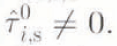
which corresponds to the shallow-ice approximation of the basal shear stress. With this shear stress and the prescribed values for the basal-velocity components, Equation (3.24) is used to calculate the basal value for

. Integrating up from the base yields surface values . The iteration is carried out by subsequently choosing a new value

where β is the iteration parameter.

4.1 Stability and convergence pattern

Reference MullerMuller (1991) provided a detailed analysis of the accuracy and stability of the two-dimensional algorithm for a Navier-Stokes fluid. He gave a criterion for the convergence of the iteration scheme

where M is the number of grid points in the horizontal direction, and {H} and {L} are the vertical and horizontal extents of the ice mass, respectively. Equation (4.1) suggests a strong dependence of the convergence range on the aspect ratio ϵ = {H}/{L} and the chosen longitudinal grid resolution

, The criterion in Equation (4.1) uses global quantities of the ice geometry. However, local conditions may require a smaller β to achieve convergence. This is especially true if the surface slope locally displays large longitudinal variations, such as in icefalls or near-steep glacier snouts. The iteration process must start with larger residuals when the aspect ratio is larger and, additionally, the iteration parameter β must be chosen smaller for larger ϵ, which also makes the convergence progress slower. Both effects together make the number of necessary iteration steps grow rapidly with increasing ϵ, Furthermore, if die ratio is too large, convergence cannot be achieved at all, no matter how small the iteration parameter β is chosen.

The aim of the iteration is to approach the surface-boundary condition

= 0. The convergence rate was tracked in many numerical experiments by monitoring the largest residual until this residual drops below a prescribed level. If the iteration parameter β is chosen much too large, the residuals start growing right at the beginning of the iteration. With β close to the convergence range, the iteration often starts promisingly with steadily decreasing residuals but, at a certain point, convergence becomes very slow or stops altogether. For an appropriate choice of β, the convergence progresses approximately exponentially until round-off errors stop it and the residual begins to vary randomly within the round-off error interval. For single-precision computation (eight relevant digits), the levelling-off occurs near the 1 Pa level, which is considered to be accurate enough for the convergence threshold. Figure 2 illustrates the various convergence/divergence patterns for the scaled plane-strain geometry shown in Figure 3, with an aspect ratio ϵ = 0.05 and a horizontal grid resolution of = 0.025. Although the chosen geometry may not look very natural, the behaviour of the iteration is the same as for realistic glacier geometries.

Fig. 2.

Convergence/divergence patterns for various iteration parameters: (a) β = 0.065, (b) 0.09, (c) 0.096, (d) 0.105 and (e) 0.28, The example corresponds to the scaled plane-strain cross-section as shown in Figure 2 and with an aspect ratio ϵ = 0.05. With the chosen grid resolution

= 0.025, the convergence criterion (Equation (3.31) yields β < 0.037.

4.2 Scale length

A given scaled geometry,

and in the three-dimensional case or , and in the plane-strain, approximation, represents an infinite set of affine glacier geometries. For the case of a grounded ice mass with no basal sliding, the scaled solutions only depend on the temperature distribution, represented by or , respectively, and the aspect ratio ϵ. For isothermal ice masses, Ã ≡ A₀, with given geometry and , the first-order equations only depend on one single parameter, the aspect ratio ϵ. The shallow-ice approximation becomes unique by setting ϵ = 0 in Equations (3.21)–(3.24) or in Equations (3.2)–(3.9).It is interesting to note that, in this case, the stress fields do not depend on the choice of A₀ but the velocity fields are proportional to A₀,

Fig. 3.

Scaled cross-section, fourth-order parabola

and

, used for the numerical experiments, of which the results are illustrated in Figures 4–8, The central thickness of the ice mass is 0.B{H} and its diameter 2{L}.

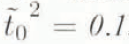
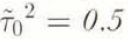
It seems reasonable to assume that the largest basal shear traction occurring in ice sheets and glaciers of a wide variety of shapes and sizes does not appreciably exceed 10⁵ Pa. It is informative to reduce the set of shallow-ice masses with a given scaled shape

and by fixing the maximum occurring basal shallow-ice shear stress at a given value T₀. The true size of an ice mass is now a function of ϵ and T₀. In this case, the scaled shallow-ice approximation is unique and thus does not depend on ϵ and T₀. From the scaling definition, Equations (2.17) and (2.19), it follows that

for the shallow ice approximation. Similarly, with Equation (2.18), it follows that u ∝ ϵ⁻¹, and w is independent of ϵ. Applying this result in Equation (3.24) yields

which indicates the growing importance of the normal deviatoric stress with growing aspect ratio ϵ. A Limiting basal shear traction of 10⁵ Pa now implies that even continent-size ice sheets cannot become thicker than a very few kilometres. On the other hand, this also implies the known fact that smaller ice masses tend to have larger aspect ratios, which makes the application of the described numerical algorithm more difficult; thus the iteration is slower for smaller glaciers than for larger ice caps and ice sheets.

This pattern is illustrated in the following numerical experiments using a simple synthetic geometry. As an example, a fourth-order parabola was chosen (Fig. 3) to represent the scaled images of the surface and basal profiles. These profiles were used in two ways. In the plane-strain approximation, they represent the geometry of a plane cross-section through an ice mass. In a second set of numerical experiments, these profiles are rotated around the

axis to define a circular ice sheet having cylindrical symmetry. Table 1 gives the scale values for {H} and {L} as a function of ϵ for this geometry and a maximum basal shallow-ice shear stress of 10⁵ Pa.

Figure 4 shows the scaled values of the basal shear stress and the longitudinal deviatoric stress at the surface, and Figure 5 shows the velocity components at the surface for the plane-strain approximation. Figures 6 and 7 show the same quantities but for the radial section along the ỹ = 0 plane of the three-dimensional geometry. As can be expected, the shear stress and the radial velocity component in the shallow-ice approximation are the for the plane-strain approximation and for the circular three-dimensional geometry. The differences between plane-strain and three-dimensional solutions of the first-order shear-stress and horizontal-velocity components are also small. However, the differences between plane-strain and the three-dimensional case are signif-icant for the radial deviatoric stress and the vertical-velocity component, which is mainly due to the spreading effect of the circular ice mass. Furthermore, deviatoric stress components and the vertical-velocity component strongly depend on the aspect ratio.

Table 1.

Scale values for {H} = 11.694/ϵ and {L} = {H}/ϵ for given ϵ for a plane-strain ice mass with scaled shape as shown in Figure 3, if the maximum occurring basal shear stress is 10⁵ Pa. The smallest possible number of iteration steps; n, the corresponding best choice for the iteration parameter β, and the largest residual

after the first iteration step ate given for some examples of ϵ and

. The theoretical upper limit for the iteration parameter β_theor (Equation (4.1) is given for comparison. The iteration was started with the shallow-ice basal shear stress and the convergence threshold was chosen at 10 Pa

The cylindrical symmetry of the assumed three-dimensional geometry should be reflected in the results for stress and velocity components. This is used to test the influence of grid size and the resulting polygonal margin of the circular ice mass. The solutions for the vertical-velocity component w and the total horizontal velocity v_h ² = u² +v² must be cylindrical. It is interesting to note that the same is true for the quadratic forms τ_rz ² = τ_xz ² + τ_yz ² and σ_rr ² = σ_yy ² + σ_xx ² + σ_xxσ_yy + τ_xy ². It is straight forward to show that the quantity σ_rz is indeed an invariant under rotations of the coordinate system around the z axis and the same holds for σ_rr, since the sum τ_rz ² + σ_rr ² equals the square of the effective stress, i.e. the second invariant of the deviatoric stress tensor. This invariance is not a result of the cylindrical symmetry of the chosen ice mass but is generally valid. Figure 8 shows a contour plot of the basal τ_rz for the circular ice sheet with cross-section as shown in Figure 3. The contours are close to circles except for a narrow marginal zone, where they seem to be influenced slightly by the polygonal shape of the margin.

Fig. 4.

Basal shear stress

and deviatoric stress

at the surface of the two-dimensional plane-strain section of the ice mass illustrated in Figure 2, for different aspect ratios: ϵ = 0.05 (solidlines), ϵ = 0.025(dashed lines) and ϵ = 0(dotted lines), and

, the horizontal coordinate axis denotes the scaled distance from the centre of the ice mass.

Fig. 5.

Horizontal velocity component ῦ and vertical velocity component

at the surface of the two-dimensional plane-strain section of the ice mass illustrated in Figure 2, for different aspect ratios: ϵ = 0.05 (solid lines), ϵ = 0.025 (dashed lines) and ϵ = 0 (dotted lines), and

= 0.1. The horizontal coordinate axis denotes the scaled distance from the centre of the ice mass.

Fig. 6.

Same as Figure 4 but in the radial cress-section along the plane ỹ = 0 of the three-dimensional circular ice mass with the cross-section illustrated in Figure 2.

Fig. 7.

Same as Figure 5 but in the radial cross-section along the plane ỹ = 0 of the three-dimensional circular ice mass with the cross-section illustrated in Figure 2.

4.3 Plane-strain parallel-sided slab

In this section, the effect of longitudinal strain on the stress components is re-investigated (Reference CollinsCollins, 1968; Reference NyeNye. 1969; Reference BuddBudd, 1970; Reference Hutter and OlunloyoHutter, 1980) by applying the first-order algorithm to a plane-strain parallel-sided slab geometry. This simple geometry is chosen to separate the effect of longitudinal strain from effects due to changes in ice thickness or longitudinal variations in the ice temperature. The coordinate system (x, z) is chosen to lie parallel to the slab direction with the z axis pointing perpendicular to the slab. The momentum equations are

where α is the inclination angle of the slab normal with respect to the direction of gravity. The same procedure as described in section 2.2 yields the corresponding first-order stress equation

For the parallel-sided slab with surface S ≡ H and base B ≡ 0, we get ∂S/∂x = 0.

The slab is defined by its thickness H and its inclination angle α, which suggests a somewhat different scaling than used in the previous sections:

where A₀ is a typical rate factor. For an isothermal slab, A ∂ A₀ , Equations (4.6) and (3.22)–(3.24) in scaled form are again with the flow law of Equation (2.10). For the slab geometry, the scaling alone yields a set of equations suitable for the first-order algorithm and the only remaining parameter is

in the flow law (·).

Fig. 8.

Contour plot of

, defined by

, at the base of the circular ice mass with the cross-section illustrated in Figure 2. The aspect ratio is ϵ = 0.05 and

. The polygonal line represents the discretized margin of the circular ice sheet.

For a parallel sided slab, the characteristic longitudinal length scale {L}, and thus the aspect ratio ϵ, can be defined by H/{L} = ϵ = sin α. With this, the stability criterion in Equation (4.1) becomes

The stability of the iteration does not depend on the slab inclination, as also can be concluded from the scaled Equations (4.10)–(4.13), which no longer contain the angle α. Moreover, convergence could only be reached for

, which limits the resolution of the longitudinal grid spacing to roughly one slab thickness. For Glen’s flow law, with , the iteration sometimes stalled, possibly due to the singularity occurring at positions where stress vanishes, e,g. near the ice surface in the locations where longitudinal strain vanishes. This is a problematic feature of the Glen flow law and confirms the necessity of knowing the flow law accurately, especially if effects of longitudinal strain are taken into account.

4.4 Effect of longitudinal strain

In the shallow-ice approximation, the shear stress is independent of longitudinal strain. This is no longer true for the first-order approximation. A look at the first-order equations for a Navier-Stokes fluid

reveals an interesting relation between longitudinal velocity variations and shear stress. With Equation (4.15), the algebraic Equation (4.13) becomes linear in

and can be solved for . Applying the solution in Equation (4.10) gives

To avoid a singularity in the shear stress,

must be finite. This not only excludes a jump in the velocity field, which is ruled out for obvious reasons, but also a jump in the longitudinal gradient of the velocity field, which is less obvious, This may explain the singular results reported by Reference Hutter and OlunloyoHutter and Olunloyo (1980) and Reference Barcilon and MacAvealBarcilon and MacAyeal (1993) for abrupt sliding/non-sliding transitions at the bed of ice slabs. With the flow law in Equation (2.10), the solutions for of the first-order Equation (4.13) also depend on , and consequently the shear stress in Equation (4.10) depends on . Thus, to avoid a singularity in the stress field, the same conditions as for a Navier-Stokes fluid must be met.

On the other hand, for a Navier Stokes fluid, the shear stress only deviates from she shallow-ice shear stress if the longitudinal gradient of the velocity field also changes with

i.e. , The same pattern holds for a generalized Glen-type fluid. Equations (4.10)–(4.13) contain only first derivatives with respect to and of the velocity components ῦ and . Therefore, if is a solution of the equations, then is also a solution, meeting the boundary conditions for stress and = 0. The constant field ῦ₀ plays a role equivalent to a global change in the sliding velocity. When the sliding velocity is a linear function of , or equivalently

a change in ῦ₀ is also equivalent to a shift of the velocity Geld parallel to the

axis, hence

To study the effect of longitudinal strain on the stress field, the shear stress and the longitudinal deviatoric stresses were calculated as a function of the prescribed longitudinal variations of the basal-velocity field. The algorithm was used to solve Equations (4.10)–(4.13) for a non-linear flow law (Equation (2.10) and n = 3. Vertical profiles of stress and velocity components were prescribed as boundary Conditions at the upper and lower ends; of the slab with finite length. Near these ends, zones with no longitudinal strain were defined by prescribing constant basal-velocity components. Between these zones, the basal-velocity components were varied as required for the specific study.

A constant longitudinal gradient of the sliding velocity, Equation (4.17), was assumed in a first set of numerical experiments. A typical result is illustrated in Figure 9. The longitudinal stress at the surface of the slab remains zero in the homogeneous zones and is constant in the zone where sliding velocity increaser; linearly. The shear stress only varies slightly in the two positions where the longitudinal gradient of the sliding velocity changes but is unaffected in places where the longitudinal sliding gradient is constant. This confirms the pattern suggested by Equation (4.16)for a Navier-Stokes fluid., in so far as shear stress is undisturbed in this case and Equations (4.18) and (4.19) still hold. The dependence of the longitudinal stress on the longitudinal sliding gradient is depicted in Figure 10.

The shear velocity, ῦ_s − ῦ_b, also depends on the longitudinal gradient of the basal velocity. This is a result of the non-linear flow law (Equation (2.10), which contains the effective stress and thus, the longitudinal deviatoric stress

, which makes the ice softer with increasing , Figure 11 illustrates the dependence of the shear velocity on the longitudinal gradient of the basal velocity for three different , together with one example of a constant viscosity (Navier-Stokes fluid), for which the shear velocity no longer depends on the sliding gradient.

This cannot hold anymore in the case of a longitudinally changing sliding gradient. In the following example, a sliding velocity is a quadratic function of

. Figure 12 shows a typical result for a constant value of , The result indicates that the longitudinal deviatoric stress is mostly determined by the local . Seemingly, the shear stress also depends mostly an the local variation of the sliding velocity: and .

Fig. 9.

Typical result for the dimensionless basal shear stress (solid line) and dimensionless longitudinal deviatoric stress at the surface of the slab versus longitudinal spatial coordinates

, given by the number of the grid point. The chosen Parameters are

(stretching) and

. The unit on the

axis corresponds to one slab thickness.

Fig. 10.

Dimensionless longitudinal deviatoric stress at the surface of the slab versus dimensionless longitudinal sliding gradient

(solid line),

(long-dashed line) and

(dashed line). The dotted line represents the result for the Navier-Stokes fluid for

.

Fig. 11.

Dimensionless shear velocity ῦ_s − ῦ_b at the surface of the slab versus dimensionless longitudinal sliding gradient

for

(solid lint),

(long-dashed line) and

(dashed line]. The dotted line represents the result for the Navier-Stokes fluid for

.