





1. Introduction
Backward stimulated Raman scattering (SRS) (Forslund, Kindel & Lindman Reference Forslund, Kindel and Lindman1975; Kruer Reference Kruer2019; Michel Reference Michel2023) is an important laser–plasma instability in inertial fusion energy (IFE) (Nuckolls et al. Reference Nuckolls, Wood, Thiessen and Zimmerman1972; Craxton et al. Reference Craxton2015; Betti & Hurricane Reference Betti and Hurricane2016). This is particularly the case for indirect drive IFE where multiple laser beams are converted into X-rays on the inner walls of a hohlraum that drive the implosion of a fuel capsule (Lindl Reference Lindl1995). In this three-wave process, an incident light wave decays into a lower-frequency, counterpropagating light wave and a forward-propagating electron plasma wave (EPW). Stimulated Raman scattering can redirect laser energy before it reaches the hohlraum wall, thus altering the spatial pattern of energy deposition, and it can generate hot electrons that preheat the capsule and reduce compression (Haan et al. Reference Haan2011). These effects make SRS a persistent concern for indirect drive IFE, particularly for designs that contain extended regions of gas fill (underdense plasma) that prevents the ablating walls from blocking the incoming lasers (Lindl Reference Lindl1995). Recent progress at the National Ignition Facility (NIF) has renewed interest in designs with higher coupling efficiency, robustness and gain (Haynam et al. Reference Haynam2007; Abu-Shawareb et al. Reference Abu-Shawareb2022; Kritcher et al. Reference Kritcher2022; Zylstra et al. Reference Zylstra2022). Because avoiding long plasma scale lengths can constrain such designs, a predictive understanding of SRS and practical methods for controlling it remain important (Myatt et al. Reference Myatt2014; Rosenberg et al. Reference Rosenberg2018).
Externally applied magnetic fields offer one possible means of modifying laser–plasma interactions. Fields aligned with the laser or hohlraum axis can alter heat transport, hot-electron propagation, cross-speckle coupling and hohlraum hydrodynamics (Yin et al. Reference Yin, Albright, Rose, Montgomery, Kline, Kirkwood, Michel, Bowers and Bergen2013; Montgomery et al. Reference Montgomery2015; Strozzi et al. Reference Strozzi, Perkins, Marinak, Larson, Koning and Logan2015). Magnetic fields are also being investigated as a way to reduce thermal losses from the fuel and increase hot-spot temperature and fusion yield (Chang et al. Reference Chang, Fiksel, Hohenberger, Knauer, Betti, Marshall, Meyerhofer, Séguin and Petrasso2011; Hohenberger et al. Reference Hohenberger, Chang, Fiksel, Knauer, Betti, Marshall, Meyerhofer, Séguin and Petrasso2012; Perkins et al. Reference Perkins, Ho, Logan, Zimmerman, Rhodes, Strozzi, Blackfield and Hawkins2017; Moody et al. Reference Moody2022a ; Walsh et al. Reference Walsh2022; Walsh et al. Reference Walsh2025). This strategy has been applied in recent NIF experiments to designs with minimal gas fill to limit SRS; future studies could extend it to higher-gain designs with increased gas-fill density (Moody et al. Reference Moody2022b ). Of particular relevance here, Winjum, Tsung & Mori (Reference Winjum, Tsung and Mori2018) used particle-in-cell (PIC) simulations to show that a field of order tens of Tesla, oriented perpendicular to the laser propagation direction, can suppress backward SRS in an IFE-relevant kinetic regime. A reduction of SRS under a transverse 13 T field was subsequently observed experimentally by Bolaños et al. (Reference Bolaños2025).
Although these fields are large in absolute units, they are small relative to the characteristic nonlinear optics of plasmas-related frequencies. We use ‘small’ or ‘weak’ to denote the ordering
 $\omega _c/\omega _p \ll 1$
, where
 $\omega _c=\mathrm{e} B/(m\mathrm{c})$
is the electron cyclotron frequency and
 $\omega _p=(4\pi n_e\mathrm{e}^2/m)^{1/2}$
is the plasma frequency. For
 $n_e/n_c\simeq 0.12$
and
 $\lambda _0={0.351}\unicode{x03BC} {\textrm {m}}$
, a 10 T field gives
 $\omega _c/\omega _p\sim 10^{-3}$
. In the cases considered here,
 $\omega _c$
is also smaller than the EPW bounce frequency,
 $\omega _b=(\mathrm{e} kE_0/m)^{1/2}$
(Morales & O’neil Reference Morales and O’neil1972), and the characteristic SRS growth and EPW damping rates. Because the EPW evolves and damps before electrons complete cyclotron orbits, an interpretation in terms of undamped Bernstein waves is not appropriate in this limit. Consistent with this ordering, the corrections to the linear Bohm–Gross dispersion relation and Landau damping rate are small (Sagdeev & Shapiro Reference Sagdeev and Shapiro1973; Lee Reference Lee2025).
The nonlinear response can nevertheless be substantial. For a large-amplitude EPW propagating across a weak magnetic field, resonant electrons are accelerated across the wave phase fronts and can be detrapped before a long-lived, Bernstein–Greene–Kruskal (BGK)-like state forms (Bernstein, Greene & Kruskal Reference Bernstein, Greene and Kruskal1957; Morales & O’neil Reference Morales and O’neil1972). The electrons thereby continue to extract energy from the wave, producing enhanced nonlinear damping even when the linear magnetic correction is negligible (Sagdeev & Shapiro Reference Sagdeev and Shapiro1973; Dawson et al. Reference Dawson, Decyk, Huff, Jechart, Katsouleas, Leboeuf, Lembege, Martinez, Ohsawa and Ratliff1983).
The nonlinear evolution of EPWs can play a critical role in the dynamics of SRS, particularly in the IFE-relevant plasmas where SRS is in the kinetic inflation regime (Vu, DuBois & Bezzerides Reference Vu, DuBois and Bezzerides2007; Ellis et al. Reference Ellis, Strozzi, Winjum, Tsung, Grismayer, Mori, Fahlen and Williams2012). Reflectivity from SRS can greatly exceed that which is predicted by linear theory in this regime, which is mainly characterised by two normalised parameters. First,
 $k\lambda _{De} \gtrsim 0.3$
, where
 $k$
is the EPW wavenumber and
 $\lambda _{De}$
is the electron Debye length, such that Landau damping is important. This is the kinetic regime. Second,
 $\gamma _0/\gamma _p \ll 1$
, where
 $\gamma _0$
is the temporal growth rate for SRS (Forslund et al. Reference Forslund, Kindel and Lindman1975) and
 $\gamma _p$
is the Landau damping rate of the EPW. This is the strongly damped regime for temporal growth. In the strongly damped regime, the temporal growth rate is given by
 $\gamma _0^2/\gamma _p$
, and linear theory predicts limited reflectivity from SRS. However, if EPWs are driven to a large enough amplitude such that
 $\omega _b/\gamma _p \gg 1$
, then resonant wave–particle interactions can cause nonlinear flattening of the distribution function near the EPW phase velocity before they dissipate due to linear Landau damping. Electron plasma waves thus evolve towards a BGK or BGK-like mode (Bernstein et al. Reference Bernstein, Greene and Kruskal1957) whose kinetic damping rate is dramatically decreased, i.e.
 $\gamma _p \to 0$
(O’neil Reference O’neil1965; Morales & O’neil Reference Morales and O’neil1972). As a result,
 $\gamma _0/\gamma _p$
can evolve to become much larger than unity, causing SRS to transition out of the strongly damped regime into a weakly damped convective regime (Vu et al. Reference Vu, DuBois and Bezzerides2007), or even an absolutely unstable (Winjum Reference Winjum2010) regime, where growth rates and reflectivity are higher.
For a laser pulse length much longer than the interaction length (
 $\equiv x_{\mathrm{max}}$
), a corresponding spatial criterion is more relevant. The condition to be in the strongly damped spatial regime is
 $(\gamma _0/\gamma _p)(v_{g2}/v_{g1})^{1/2}\lt 1$
, where
 $v_{g2}$
and
 $v_{g1}$
are the group velocities of the EPW and scattered light wave, respectively. In this regime the gain is given by
 $\varGamma x_{\max }$
, where
 $\varGamma =\gamma _0^2/(\gamma _p v_{g1})$
(Forslund et al. Reference Forslund, Kindel and Lindman1975; Michel Reference Michel2023). When
 $\varGamma x_{\text{max}} \lesssim 1$
, the interaction length is not large enough for the pump to convectively drive plasma waves to amplitudes for which kinetic inflation can occur (Winjum Reference Winjum2010). When
 $\varGamma x_{\max }\gtrsim 1$
–
 $2$
, inflationary SRS can occur. When
 $\varGamma x_{\max }\gg 1$
and
 $(\gamma _0/\gamma _p)(v_{g2}/v_{g1})^{1/2}\lt 1$
, substantial amplification can occur even without inflation.
These criteria identify the range of speckle intensities for which changes to nonlinear EPW damping can strongly affect SRS reflectivity. Here, small perpendicular magnetic fields can mitigate SRS in the kinetic inflation regime by enhancing the damping of nonlinear EPWs and disrupting the process of kinetic inflation, as demonstrated by the simulations of Winjum et al. (Reference Winjum, Tsung and Mori2018), which established magnetic mitigation at intensities representative of a high-intensity laser speckle. A smoothed high-power laser beam, however, contains speckles over a range of intensities from those near the kinetic inflation threshold to those that have substantially larger peak intensities. It is not evident that magnetic suppression persists throughout the intensity distribution, nor that the enhanced damping mechanism persists in two dimensions across all intensities, given finite width effects such as transverse particle loss and wavefront evolution of SRS in a realistic speckle. The present work addresses these questions by following both the underlying EPW dynamics and self-consistent SRS from below the inflation threshold to well above it.
We use one-dimensional (1D) and two-dimensional (2D) Osiris PIC simulations (Fonseca et al. Reference Fonseca2002) of externally driven EPWs and continuously driven backward SRS. The driven EPW simulations isolate the nonlinear damping and phase-space dynamics, while the self-consistent SRS simulations determine their consequences for reflectivity and burst recurrence. The SRS simulations use
 $k\lambda _D\simeq 0.30$
and span
 $a_0=0.004$
–
 $0.028$
, corresponding to
 $\gamma _0/\gamma _p=0.16$
–
 $1.11$
and
 $\varGamma x_{\max }=0.4$
–
 $20.2$
. We compare unmagnetised plasmas with transverse fields satisfying
 $\omega _c/\omega _p=0.003$
and 0.006; in two dimensions, both in-plane and out-of-plane transverse field orientations are considered.
The results reveal three intensity regimes. At intensities near the unmagnetised threshold the application of a magnetic field suppresses inflationary SRS. At intermediate intensities where substantial growth occurs in unmagnetised plasmas, an applied magnetic field reduces the time-averaged reflectivity, by factors of approximately two to three in one dimension. At even higher intensities, where
 $\gamma _0/\gamma _p \gtrsim 1$
, the process of kinetic inflation becomes less important to the growth of SRS, so the difference in average reflectivity narrows; magnetised values can become comparable to or even slightly larger than unmagnetised values. Thus, a weak transverse field does not suppress SRS across all intensities. Even where the average reflectivities are similar, however, the instability retains distinct magnetic signatures. Without a field, long-lived, frequency-shifted EPW packets and a persistently modified distribution function influence subsequent bursts, producing irregular recurrence. A transverse field enhances EPW damping, limits resonant flattening and the nonlinear frequency shift, and reduces the memory of previous bursts, producing a more regular recurrence pattern.
Two-dimensional geometry makes the EPW evolution more complex. Transverse localisation and finite spot size can prevent an unmagnetised EPW from becoming fully undamped, while particle side loss, wavefront curvature, filamentation and the trapped particle instability (TPI) reduce the contrast between magnetised and unmagnetised damping. Nevertheless, the principal intensity dependence of SRS is preserved: the field raises the inflation threshold, lowers reflectivity near the threshold and has a diminishing effect on average reflectivity far above the threshold. Moreover, the recurrence remains distinctly more regular in the magnetised cases even when the EPW damping rates are similar. This demonstrates that both EPW damping and relaxation of the resonant electron distribution govern the long-time dynamics of kinetic SRS.
The remainder of the paper is organised as follows. Section 2.1 examines the nonlinear evolution of driven EPWs in one dimension and § 2.2 relates that evolution to self-consistent 1D SRS. Section 3 then treats geometrical effects using 2D driven EPW and single-speckle SRS simulations. Section 4 summarises the results and discusses directions for future work.
2. One-dimensional simulation results
2.1. One-dimensional driven EPW simulations
As described above, while a sufficiently small normalised transverse magnetic field has little effect on the linear behaviour of EPWs, it can have a profound effect on the nonlinear behaviour of EPWs. In this section we begin with a short description of single electron motion in an EPW propagating perpendicular to a magnetic field, and then present 1D PIC simulation results to demonstrate key physics. The aim of the simulations in this section is not to provide a broad parameter scan, but rather to examine parameters of relevance to the self-consistent simulations of backward SRS to follow.
We assume an EPW of the form
 $\boldsymbol{E} = \hat {\boldsymbol{x}} E_0 \sin (kx - \omega t)$
, described by a scalar potential
 $\phi = \phi _0 \cos (kx - \omega t)$
propagating across a magnetic field oriented along the
 $\hat {\boldsymbol{z}}$
direction,
 $\boldsymbol{B} = \hat {\boldsymbol{z}} B_0$
. The equations of motion are thus given by
 \begin{equation} m \frac {\mathrm{d} v_x}{\mathrm{d} t} = -\mathrm{e} \left (E_0 \sin (kx-\omega t) + \frac {v_y}{\mathrm{c}}B_0\right ), \end{equation}
 \begin{equation} m \frac {\mathrm{d} v_y}{\mathrm{d} t} = \mathrm{e} \frac {v_x}{\mathrm{c}}B_0. \end{equation}
Consider an electron initially trapped in the EPW with
 $v_x \approx v_\varphi$
, where
 $v_\varphi \equiv \omega /k$
is the phase velocity of the wave. This electron is accelerated along
 $v_y$
with an average force
 $\sim \mathrm{e} ({v_\varphi }/{\mathrm{c}}) B_0$
. As
 $v_y$
increases in time, the magnetic field produces a backward force in the
 $\hat {\boldsymbol{x}}$
direction. The electron thus executes bounce motion in the
 $\hat {\boldsymbol{x}}$
direction about a location (phase) in the wave where
 $E_0 \sin (kx')+ ({v_y}/{\mathrm{c}})B_0\approx 0$
and
 $x' \equiv x - v_\varphi t$
is the location of the particle in the wave frame. Eventually,
 $({v_y}/{\mathrm{c}})B_0$
increases to a value larger than
 $E_0$
, at which point the electron detraps with a total speed
 $\approx \sqrt {v_\varphi ^2 + ({E_0}/{B_0})^2}$
and subsequently executes cyclotron motion (Dawson et al. Reference Dawson, Decyk, Huff, Jechart, Katsouleas, Leboeuf, Lembege, Martinez, Ohsawa and Ratliff1983). For the parameters of interest in this work,
 $E_0 / B_0 \gg v_\varphi$
, indicating that this process can lead to energetic electrons and strong damping of the EPW. Furthermore, in some cases,
 $E_0 / B_0 \gt \mathrm{c}$
and so acceleration can occur indefinitely (Katsouleas & Dawson Reference Katsouleas and Dawson1983). In reality, the energy is limited by the plasma wave damping or breaking apart from trapped particle sideband instabilities (Kruer, Dawson & Sudan Reference Kruer, Dawson and Sudan1969; Brunner & Valeo Reference Brunner and Valeo2004), or electrons transiting the wavefront for a finite width wave. In this regime, relativistic electrons can be produced and, thus, a relativistic analysis is required. More details of the single electron dynamics and pertinent time scales are given in Appendix A. Finally, we note that in the remainder of the text the coordinate system will be referred to using the notation
 $\hat {\boldsymbol{x}}_1$
,
 $\hat {\boldsymbol{x}}_2$
,
 $\hat {\boldsymbol{x}}_3$
instead of
 $\hat {\boldsymbol{x}}$
,
 $\hat {\boldsymbol{y}}$
,
 $\hat {\boldsymbol{z}}$
.
In the remainder of this section, we rely on 1D PIC simulations using Osiris (Fonseca et al. Reference Fonseca2002) of nonlinear EPWs to study how small magnetic fields impact their evolution. In these simulations the EPWs are impulsively driven by a ponderomotive (external) force of short duration. The ponderomotive driver has the form
 $E_{\mathrm{ext}}(x_1, t) = E_d(t) \sin (k_1 x_1 - \omega t)$
, where
 $E_d(t) = ({t}/{\tau })E_{d0}$
if
 $t\lt \tau$
,
 $({(2\tau -t)}/{\tau } )E_{d0}$
if
 $\tau \lt t \lt 2\tau$
and 0 otherwise. The impulse (i.e. amplitude,
 $E_{d0}$
, and duration,
 $\tau$
) of the driver is chosen such that the resulting EPWs correspond with those observed in self-consistent simulations of SRS shown in § 2.2. In particular, we use
 $\omega _p \tau \approx 10$
, so that the driver amplitude is 0 by
 $\omega _p t = 20$
and EPWs are undriven thereafter (
 $\omega _p t_{\mathrm{max}} = 1000$
). Other forms for
 $E_d(t)$
have been used and the results do not change. In what follows, results for waves of two different peak amplitudes are shown.
First, results are shown for a relatively small-amplitude wave that reaches a peak amplitude of
 $\omega _b^2 / \omega _p^2 = 0.014$
and is roughly 10 times smaller than the maximum EPW amplitude observed in the SRS simulations described below. Note that
 $\omega _b^2/\omega _p^2 \approx \omega _b^2/\omega \omega _p \equiv \mathrm{e} E_0/mv_{\varphi }\omega _p \equiv \bar E$
. In these units, for
 $k\lambda _D=0.32$
, the Coffey wavebreaking limit (Dawson Reference Dawson1959; Coffey Reference Coffey1971) for the electric field is
 $\bar E_{WB} = 0.19$
, where
 $\lambda _D\equiv v_{th}/\omega _p$
is the Debye length. Such small-amplitude waves, where
 $\bar E \ll \bar E_{WB}$
, play an important role in the onset and growth of the instability. Second, results are shown for a wave that reaches a peak amplitude of
 $\omega _b^2 / \omega _p^2 = 0.130$
, which is approximately equal to the largest amplitude EPWs observed in SRS simulations and is approaching the Coffey limit.
The plasma has a uniform density and a temperature of 2.56 keV corresponding to
 $v_{th}/\mathrm{c}=0.071$
. The wavenumber of the driver is
 $k_1=4.49 \omega _p/\mathrm{c}$
, corresponding to
 $k\lambda _D=0.32$
. The driver frequency is
 $\omega = 1.142 \omega _p$
, chosen to match the Bohm–Gross dispersion relation.
Two box lengths are simulated. First, a single-wavelength box (
 $x_{\text{max}} = 19.72 \lambda _D)$
is used to isolate the driven mode. This simulation contains 98 cells, with
 $\Delta x = 0.2 \lambda _D$
and
 $\omega _p \Delta t = 0.014$
. For this small cell size, the numerical correction to the Bohm–Gross dispersion relation is small. Second, a 100-wavelength box (
 $x_{\text{max}} = 1972 \lambda _D$
) is simulated, where the cell size and time step are again,
 $\Delta x = 0.2 \lambda _D$
and
 $\omega _p \Delta t = 0.014$
. The use of a longer simulation domain allows for the growth of the sideband instability (Kruer et al. Reference Kruer, Dawson and Sudan1969; Brunner & Valeo Reference Brunner and Valeo2004), which can play a very important role in the nonlinear evolution of an EPW. We show below that this takes energy from the driven mode, and leads to earlier detrapping and a reduction in the peak energy of trapped electrons. In each case,
 $10^6$
particles per cell (ppc) are used with cubic particle shapes. The ions are stationary. Periodic boundary conditions are used for fields and particles.
Binary Coulomb collisions are neglected in this work; for the densities and temperatures considered here, their rates are small compared with the other frequencies and rates of interest, namely the electron bounce frequency, the Landau damping rate, the electron cyclotron frequency and the temporal SRS growth rate. In order to ensure that finite size particle interactions (collisions between PIC particles) are also not important, we have also redone some driven EPW simulations with the same number of particles per cell as in the self-consistent SRS simulations. As commented below, EPWs evolve to undamped modes for these simulations as well indicating that PIC particle collisions are not modifying the physics.
External magnetic fields are applied in positive
 $\hat {\boldsymbol{x}}_3$
and have magnitudes
 $\omega _c / \omega _p = 0.003$
and 0.006. We introduce the notation
 $\bar B_{\mathrm{ext}} \equiv \omega _c/\omega _p$
to be used as a shorthand. As with the driver parameters, the magnetic field amplitude is chosen to correspond with the magnetic fields that will be used in simulations of self-consistent SRS. Assuming a laser wavelength
 $\lambda _0 = {0.351}\unicode{x03BC} {\textrm {m}}$
, and
 $n_e/n_c = 0.12$
, the normalised magnetic field amplitudes of
 $\omega _c / \omega _p = 0.003$
and
 $0.006$
correspond with 30 T and 60 T, respectively.
We begin by showing in figure 1 the time evolution of the EPW amplitude,
 $[E_1]$
, for cases with
 $\bar B_{\mathrm{ext}} =$
0, 0.003 and 0.006 at the lower of the two amplitudes (
 $\omega _b^2 / \omega _p^2 = 0.014$
). Mode amplitude is obtained by averaging the magnitude of the longitudinal field over the length of the box, i.e.
 $[E_1](t) \equiv ({\pi }/{2}) \int _0^{x_{\text{max}}} {\rm d}x_1 |E_1(x_1,t)| / x_{\text{max}}$
. The scaling factor of
 $\pi /2$
ensures that the maximum value of
 $[E_1]$
is equal to the maximum value of
 $E_1$
, assuming that the electric field is of the form
 $E_0 \sin (kx-\omega t)$
and the box has an integer number of wavelengths. The single-wavelength cases are shown by the solid lines and the 100-wavelength cases are shown by the dashed lines.
Amplitude versus time of EPWs in a 1D system for different external magnetic field amplitudes in a single-wavelength box (solid lines) and a 100-wavelength box (dashed lines). A ponderomotive driver is used over the first
 $\omega _p t = 20$
to excite the wave, which reach a maximum amplitude of
 $\omega _b^2/\omega _p^2 = 0.014$
.

First, for the single-wavelength cases (shown by the solid lines in figure 1), after the driver is turned off at
 $\omega _p t \approx 20$
linear Landau damping is observed regardless of the magnetic field amplitude. For these parameters,
 $\omega _b/\gamma _p=3.7$
, so that nonlinear effects arise before significant Landau damping has arisen. After this initial linear Landau damping, however, the behaviour differs with and without a magnetic field.
In the unmagnetised case, after the driver is turned off and once nonlinear effects take hold, oscillations in
 $[E_1]$
are seen at roughly the trapped particle bounce frequency as particles alternately give energy to and take energy from the wave. The oscillations will not be exactly at the bounce frequency but at a lower frequency, as some electrons with higher energies in the wave frame have longer periods (nonlinear oscillations) determined by elliptic functions. As they bounce, phase mixing occurs and the damping rate ultimately vanishes (O’neil Reference O’neil1965; Morales & O’neil Reference Morales and O’neil1972). Simulations with
 $\omega _b/\gamma _p \ll 1$
and
 $\sim 1$
were also performed and confirm that when the damping rate sufficiently exceeds the bounce frequency, the wave damps before it can evolve into an undamped mode. We note that the amplitude oscillations persist over the entire duration of the simulation. It would be expected that they cease after a few oscillations. This is an area for future investigation.
With a magnetic field, the behaviour is profoundly different despite the small normalised magnitude of the EPW. For both
 $\bar B_{\mathrm{ext}} =$
0.003 and 0.006, oscillations are initially observed at a slightly modified bounce frequency (
 $\approx \sqrt {\omega _b^2+\omega _c^2}$
), as described by Dawson et al. (Reference Dawson, Decyk, Huff, Jechart, Katsouleas, Leboeuf, Lembege, Martinez, Ohsawa and Ratliff1983) and discussed in Appendix A. In particular, we note that the bounce frequency is increased in the presence of the magnetic field despite a decreased EPW amplitude (which would otherwise result in a decrease in the bounce frequency), clearly showing evidence of the effect of the magnetic field.
Oscillations at the modified bounce frequency are followed by damping of the wave – evolution to an undamped mode is not seen. This is due to the fact that, as described previously, particles continuously extract energy from the wave as they are accelerated by the magnetic field across the phase front – even when they move backwards in the wave’s frame. The damping of the wave is not exponential and it is similar for the two values of
 $\bar B_{\mathrm{ext}}$
. For the larger value of
 $\bar B_{\mathrm{ext}}$
, the wave damps to zero amplitude.
Wavenumber versus time of EPWs in a 1D, 100-wavelength long box for different external magnetic field amplitudes. A ponderomotive driver is used over the first
 $\omega _p t = 20$
to excite the wave, which reach a maximum amplitude of
 $\omega _b^2/\omega _p^2 = 0.014$
. The driver has a wavenumber of
 $k=4.487 \omega _0 / c$
. Evidence of the sideband instability is seen primarily for
 $\bar B_{\mathrm{ext}} = 0$
.

As mentioned above, the single-wavelength simulations do not have sufficient resolution in
 $k$
space to allow for growth of the sideband instability (Kruer et al. Reference Kruer, Dawson and Sudan1969; Brunner & Valeo Reference Brunner and Valeo2004), which can impact EPW dynamics. The dashed lines in figure 1 show mode amplitude,
 $[E_1]$
, versus time for the 100-wavelength box. In addition, a plot of the wavenumber
 $(k_1)$
versus time is shown in figure 2 for this case. The resolution in
 $k$
space is
 $\Delta k = 0.0449 \omega _p / c$
.
For
 $\bar B_{\mathrm{ext}} =$
0, it can be seen in figure 2(a) that sidebands begin to develop between
 $\omega _p t \approx 200$
and
 $\omega _p t \approx 400$
, mainly at
 $k = 4.0 \omega _p / c$
, the
 $k$
mode nearest to the driven mode. They saturate at
 $t\omega _p \approx 600$
at an amplitude comparable to the driven mode. This corresponds with a roughly
 $17\,\%$
decrease in the average mode amplitude between
 $\omega _p t\approx 400$
and
 $\omega _p t \approx 600$
as seen by the dashed lines in figure 1. After saturation of the sidebands, no further decrease in the driven mode amplitude is seen. Amplitude oscillations due to electron bounce motion also cease at this time – a result of more rapid phase mixing that occurs in the presence of multiple EPW modes.
For
 $\bar B_{\mathrm{ext}} =$
0.003, sidebands are seen, however, their amplitude is at most an order of magnitude smaller than the driven mode. For
 $\bar B_{\mathrm{ext}}=0.006$
, only minimal sideband growth is seen in figure 2(c); this is likely because the driven modes damp sufficiently before sidebands can emerge. Therefore, the evolution of the driven modes with the external magnetic field in figure 1 is nearly identical in the multi-wavelength (dashed lines) and single-wavelength cases (solid lines). Thus, we conclude that, for the parameters of relevance to SRS in IFE plasmas, while the sideband instability does clearly play a role in nonlinear EPW evolution, it does not alter the main conclusions. Namely, the EPW still evolves to an undamped mode for
 $\bar B_{\mathrm{ext}}=0$
, and enhanced damping occurs over relatively short time scales (
 $\sim 100 \omega _p^{-1}$
) when a small normalised magnetic field is applied.
Amplitude versus time of EPWs in a 1D system for different external magnetic field amplitudes in a single-wavelength box (solid lines) and a 100-wavelength box (dashed lines). A ponderomotive driver is used over the first
 $\omega _p t = 20$
to excite the waves, which reach a maximum amplitude of
 $\omega _b^2 / \omega _p^2 = 0.130$
.

The qualitative behaviours observed above in the low-amplitude (
 $\omega _b^2 / \omega _p^2 = 0.014$
), single- and multi-wavelength simulations also hold in the high-amplitude simulations (
 $\omega _b^2 / \omega _p^2 = 0.130$
). Specifically, evolution to an undamped mode is seen with
 $\bar B_{\mathrm{ext}}=0$
and damping is seen due to an external magnetic field, and this behaviour is not altered by the presence of the sideband instability. This is illustrated in figure 3, which shows mode amplitude,
 $[E_1]$
, versus time for cases with
 $\bar B_{\mathrm{ext}} =$
0, 0.003 and 0.006. The single-wavelength results are shown by the solid lines. Multi-wavelength results are shown by the dashed lines, where the box length is 10 wavelengths. Note that the resolution in
 $k$
space in the multi-wavelength case is
 $\Delta k = 0.4488 \omega _p / c$
, which is coarser than in the multi-wavelength simulation at low amplitude discussed above. This was found to be sufficient to enable sideband growth, while this was not the case at the lower amplitude.
Quantitatively, the damping rate is lower in the high-amplitude simulations for the single-wavelength box. For instance, for
 $\bar B_{\mathrm{ext}}=0.003$
and low amplitude, a decay from the peak EPW amplitude of roughly 75 % is seen by
 $\omega _p t = 400$
(from
 $\omega _b^2 / \omega _p^2 =$
0.014 to 0.004) as seen by the solid lines in figure 1. By contrast, in the high-amplitude case, by
 $\omega _p t = 400$
only a reduction of 35 % has occurred (from
 $\omega _b^2 / \omega _p^2 =$
0.130 to 0.084) as seen by the solid lines in figure 3. Similarly, for
 $\bar B_{\mathrm{ext}} = 0.006$
, by
 $\omega _p t = 400$
the decay is roughly 79 % in the low-amplitude case versus only 50 % in the high-amplitude case. Furthermore, whereas in the low-amplitude case the EPW has vanished or nearly vanished by the end of the simulated time (
 $\omega _p t = 1000$
), in the high-amplitude case the EPW amplitude remains appreciable.
The sideband instability is far more impactful at high EPW amplitudes. At the low amplitude, minimal sidebands were present (as seen in figure 2) and these did not impact the temporal evolution of the amplitude of the wave (as seen by the dashed lines in figure 1). At the high amplitude on the other hand, although not shown directly, a significant growth of sidebands occurred in both the cases with
 $\bar B_{\mathrm{ext}}=$
0.003 and 0.006, and the amplitude of the sidebands is comparable to that of the driven mode. Thus, their presence does impact the temporal evolution of the amplitude of the wave, as can be seen by the dashed lines in figure 3. An increased damping of the wave is evident, and final wave amplitudes of
 $\omega _b^2 / \omega _p^2 \approx 0.0025$
are seen for both
 $\bar B_{\mathrm{ext}} = 0.003$
and 0.006.
Projection of electron phase space showing differences in trapping, and acceleration and detrapping due to the magnetic field across a variety of 1D simulations of driven EPWs: (a) single-wavelength box, high-amplitude plasma wave (
 $\omega _b^2 / \omega _p^2 = 0.130$
),
 $\bar B_{\mathrm{ext}} = 0$
; (b) single-wavelength box, high-amplitude plasma wave (
 $\omega _b^2 / \omega _p^2 = 0.130$
),
 $\bar B_{\mathrm{ext}} = 0.006$
; (c) single-wavelength box, low-amplitude plasma wave (
 $\omega _b^2 / \omega _p^2 = 0.014$
),
 $\bar B_{\mathrm{ext}} = 0.006$
; (d) 10-wavelength box, high-amplitude plasma wave (
 $\omega _b^2 / \omega _p^2 = 0.130$
),
 $\bar B_{\mathrm{ext}} = 0.006$
.

Finally, in addition to the differences described above, electrons can escape with a much higher energy in the high-amplitude case. As described above and in Appendix A, electrons escape the wave when the magnetic force,
 $e ({v_2}/{c})B_0$
, is larger than the peak electric force of the wave,
 $eE_0$
. To lowest order, the electrons thus escape with a speed,
 $ {v_{\mathrm{esc}}}/{c} = {E_0}/{B_0}= ({\omega _b^2}/{\omega \omega _p}) ({\omega _p}/{\omega _c}) ( {v_{\varphi }}/{c}) \approx \bar E_{EPW} ({\omega _p}/{\omega _c}) ({v_\varphi }/{c})$
(Sugihara & Midzuno Reference Sugihara and Midzuno1979; Dawson et al. Reference Dawson, Decyk, Huff, Jechart, Katsouleas, Leboeuf, Lembege, Martinez, Ohsawa and Ratliff1983). Since the ratio
 $E_0/B_0$
exceeds unity in the high-amplitude simulations, this implies that electrons cannot escape and ‘unlimited’ acceleration can in principle be achieved (Katsouleas & Dawson Reference Katsouleas and Dawson1983).
With this in mind, energetic electron generation is investigated in figure 4, where a project of electron phase space in
 $u_1-u_2$
space is shown near the end of the simulation at a time
 $\omega _0 t = 828.24$
, where
 $u_i$
is the proper velocity in the
 $x_i$
direction. In figure 4(a), results from the high-amplitude, single-wavelength case with
 $\bar B_{\mathrm{ext}}=0$
are shown. Modification, or flattening, of the electron distribution for
 $u_1$
near the phase velocity (
 $v_\varphi = 0.255 c$
or
 $u_\varphi =0.263c$
) due to resonant wave–particle interactions can be seen. Electrons do not detrap since the wave is undamped.
In figure 4(b), results from the high-amplitude, single-wavelength case with
 $\bar B_{\mathrm{ext}} = 0.006$
are shown. Here,
 $E_0/B_0 = 4.8$
, so unlimited acceleration can occur for some initially trapped electrons. Detrapping occurs over a range of proper speeds (where hereafter, the term ‘proper speed’ refers to the magnitude of the proper velocity,
 $|\boldsymbol{u}|$
), depending on the initial conditions (
 $C_0 \equiv v_{y0} - \omega _c x_0'$
in Appendix A). When electrons detrap, they rotate (clockwise) in phase space. There is thus a distribution of detrapping times that map to the amount of phase-space rotation, giving rise to the spiral shape that is evident in the figure. Those electrons that detrap first are those that have been least accelerated transversely, and at the time plotted, they have rotated the most and are still attached to the main body of the electron distribution function. Over time, more electrons continue to detrap and rotate in phase space. Eventually, only electrons with initial
 $u_1 \approx u_{\varphi }$
remain trapped. This group has detached from the main body of the distribution function and acquires relativistic energies (
 $u_1 \gtrsim c$
). Although cut off in the figure, some electrons remain trapped at the end of the simulation and continue to be accelerated to proper speeds exceeding
 $u=1.5 c$
. Despite such energetic electron generation, we note that modifications to the
 $u_1$
distribution function at
 $u_1 \sim u_\varphi$
are minimal when compared with those without a magnetic field in figure 4(a) as the trapped electrons are dispersed to a larger range of proper velocities.
In figure 4(c), results from the low-amplitude, single-wavelength case with
 $\bar B_{\mathrm{ext}} = 0.006$
are shown. For clarity, this data is from the same simulation as shown by the solid line for
 $\bar B_{\mathrm{ext}} = 0.006$
in figure 1. Here,
 $E_0/B_0 = 0.5$
, thus, the upper bound for the trapped electron escape velocity in
 $\hat {\boldsymbol{x}}_2$
is
 $v_{\mathrm{esc}} = 0.5c$
and the total speed is
 $v = \sqrt {v_{\varphi }^2+v_{\mathrm{esc}}^2}=0.56c$
or proper speed
 $u=0.68 c$
. As seen in the figure, the entire population of initially trapped electrons eventually detraps and executes cyclotron motion in the clockwise direction. The peak electron proper speeds are
 $u\approx 0.6$
, slightly less than the theoretical peak likely due to the fact that the wave damps and allows electrons to detrap prematurely. Again, modifications to the
 $u_1$
distribution function near
 $u_\varphi$
are much less than without a magnetic field.
Finally, in figure 4(d), results from the high-amplitude, multi-wavelength case with
 $\bar B_{\mathrm{ext}} = 0.006$
is shown. The box is 10 wavelengths long, allowing for the growth of the sideband instability. In this case, since the wave amplitude is modulated by sidebands, particle acceleration is limited when compared with the single-wavelength case at the same amplitude (figure 4
b) since electrons can detrap upon encountering a lower amplitude portion of the modulated wave. Thus, the entire population of initially trapped electrons has detrapped by the time shown, and the peak electron proper speeds are
 $u\approx 0.8 c$
instead of in excess of
 $1.5c$
as in the single-wavelength case. Again, modifications to the
 $u_1$
distribution function near
 $u_\varphi$
are much less than without a magnetic field.
In the simulations discussed so far in this section,
 $10^6$
ppc were used. This was done to increase the signal-to-noise ratio for purposes of illustration. However, the self-consistent simulations of SRS that will be shown later – and which the above results are intended to inform – use only 512 ppc. Thus, to ensure that PIC particle interactions do not lead to significant collisional damping, we investigate whether the phenomena observed above are still present with only 512 ppc. Figure 5 compares mode amplitude versus time at
 $10^6$
versus 512 ppc for the small-amplitude (
 $\omega _b^2 / \omega _p^2 = 0.014$
), single-wavelength case, for
 $\bar B_{\mathrm{ext}} = 0$
in panel (a) and
 $\bar B_{\mathrm{ext}} = 0.006$
in panel (b). The dashed orange curves represent the same data as shown by the solid lines in figure 1 (i.e.
 $10^6$
ppc are used). The solid blue curves represent an ensemble average over 10 simulations, each with 512 ppc and each initialised with a different random number generator seed. The ensemble average is obtained by averaging the magnitude of the longitudinal field over the length of the box for each case (in the same way as for the
 $10^6$
ppc cases), and averaging over the ensemble.
Amplitude versus time of EPWs in a 1D, single-wavelength system for
 $\bar B_{\mathrm{ext}}$
=0 (a) and
 $\bar B_{\mathrm{ext}}$
=0.006 (b). A ponderomotive driver is used over the first
 $\omega _p t = 20$
to excite the waves, which reach a maximum amplitude of
 $\omega _b^2 / \omega _p^2 = 0.014$
. The dashed orange curves represent the same data as in the solid lines in figure 1, where
 $10^6$
ppc are used. The solid blue curves represent an ensemble average over 10 simulations, each with 512 ppc.

It can be seen that the same key phenomena is observed for 512 ppc. Namely, for
 $\bar B_{\mathrm{ext}}=0$
, Landau damping is observed initially, followed by oscillations at the bounce frequency, and finally, the evolution to an undamped mode. For
 $\bar B_{\mathrm{ext}}=0.006$
, an oscillation at the modified bounce frequency is still seen, followed by a rapid decay of the wave. While for 512 ppc, the wave decays to
 $\omega _b^2/\omega _p^2 \approx 0.005$
, which is half the noise level. Although the results for 512 ppc are noisier, they confirm that plasma waves excited near the noise level still behave according to collisionless physics. Last, although not shown, we note that for the large-amplitude (
 $\omega _b^2 / \omega _p^2 = 0.130$
) case, the signals are well out of the noise for 512 ppc.
2.2. One-dimensional self-consistent SRS simulations
The nonlinear evolution of EPWs that was investigated in the previous section plays a critical role in the dynamics of SRS. This is particularly true in IFE-relevant plasmas, where SRS is in and around the strongly damped kinetic regime (
 $k\lambda _D\gtrsim 0.3$
,
 $\gamma _0/\gamma _p \ll 1$
,
 $\varGamma x_{\mathrm{max}} \gtrsim 1 {-} 2$
). In the kinetic regime, reflectivity from SRS far exceeds that which is predicted by linear theory due to nonlinear EPW dynamics that cause SRS to transition from the strongly damped regime into a weakly damped convective or absolutely unstable regime. By altering nonlinear EPW dynamics, small magnetic fields disrupt the process of kinetic inflation and lead to mitigation of SRS. This was shown by Winjum et al. (Reference Winjum, Tsung and Mori2018), where moderate intensities (i.e.
 $\gamma _0/\gamma _p \ll 1$
and
 $\varGamma x_{\mathrm{max}} \gtrsim 1 - 2$
) were considered. In this section, 1D PIC simulations are shown to illustrate how the effect of the magnetic field on SRS varies as the intensity increases such that
 $\gamma _0/\gamma _p \to 1$
and
 $\varGamma x_{\mathrm{max}} \gg 1$
. As mentioned in the introduction, these intensities correspond to those found in the highest intensity speckles of a NIF beam.
We simulate an
 $f / 8$
Gaussian laser beam with wavelength
 $\lambda _0 = {0.351}\unicode{x03BC} {\textrm {m}}$
, launched from the left-hand boundary using an antenna, propagating to the right, in the positive
 $\hat {\boldsymbol{x}}_1$
direction, and polarised in
 $\hat {\boldsymbol{x}}_2$
. Although these are 1D simulations, the beam corresponds to
 $f/8$
in the sense that the box length is roughly 2 Rayleigh lengths. The laser has a rise time of
 $\omega _0 t_{\mathrm{rise}} = 100$
, and the shape of the rise is
 $6\bar t^5-15\bar t^4+10{\bar t}^3$
, where
 $\bar t\equiv t/t_{\mathrm{rise}}$
. After
 $\bar t \to 1$
the laser holds its peak value over the remainder of the simulation. A range of peak intensities is considered,
 $a_0 = 0.004 {-} 0.028$
, where
 $a_0$
is the normalised vector potential,
 $a_0 = {eA_0}/{mc^2}$
. This range corresponds to
 $\gamma _0/\gamma _p = 0.16 {-} 1.11$
and
 $\varGamma x_{\mathrm{max}} = 0.4 {-} 20.2$
. We also note that
 $a_0 = ({eE_0}/{m c \omega _0}) \equiv ({v_{osc}}/{c})$
and
 $a_0 = 0.853 \times 10^{-9} I\,({\textrm {W cm}^{-2}}) \sqrt {\lambda _0\,(\unicode{x03BC} {\textrm {m}})}$
. In physical units, this range of intensities corresponds to
 $I = {1.7 \times {10}^{14}}\,{\textrm {W cm}^{-2}}$
 $\text{to} \,\,{8.7\times {10}^{15}}\,{\textrm {W cm}^{-2}}$
. Stimulated Raman scattering is not seeded and grows from simulation noise.
The box length is
 $x_{1,\mathrm{max}} = 2148.1c/\omega _0$
and 17 900 cells are used. The time step is
 $0.114 \omega _0$
and simulations are run for a duration
 $\omega _0 t_{\mathrm{max}} = 20\,000$
. Given the laser parameters, this corresponds approximately to a box length of
 ${120}\unicode{x03BC} {\textrm {m}}$
and a duration of 4 ps. External magnetic fields are oriented in
 $\hat {\boldsymbol{x}}_3$
and have magnitudes
 $\bar B_{\mathrm{ext}} \equiv \omega _c/\omega _p = 0$
, 0.003 and 0.006, corresponding to 0, 30 T and 60 T, respectively. Open boundary conditions are used for fields and thermal boundary conditions are used for particles. In addition, we make use of Osiris’ extended particle absorber (Miller et al. Reference Miller, May, Fiuza and Mori2021) at the far right-hand edge of the box (
 $x_1=2148.1 c/\omega _0$
) to prevent the reflux of hot electrons generated from SRS EPWs.
We initialised 512 electrons per cell with a temperature of 2.56 keV (
 $v_{th} = 0.071 c$
) and a slight linear density gradient
 $n_e = 11.8{-}12.2\,\% n_c$
, giving
 $k\lambda _D \approx 0.30$
in the middle of the gradient. This slight gradient reduces the amount of forward SRS thus further isolating the physics of backward SRS and altering absolute growth. We note that, across the entire range of intensities we consider, the density gradient is small enough such that the Rosenbluth gain factor (Rosenbluth Reference Rosenbluth1972),
 $G_R$
, is always much greater than twice the spatial amplification factor,
 $(\varGamma x_{1,\mathrm{max}})$
, where
 $\varGamma$
is the strongly damped spatial growth rate of the instability (Forslund et al. Reference Forslund, Kindel and Lindman1975). Thus, gain is limited by the box length,
 $x_{1,\mathrm{max}}$
, and not the density gradient.
Ions are fixed to isolate the physics of SRS. Although not shown, simulations with mobile ions were also performed. A charge-to-mass ratio of
 $1/1836$
was used. Simulations with both cold ions (
 $ZT_e/T_i = 10$
) and warm ions (
 $ZT_e/T_i = 1$
), as well as a number of different laser intensities (
 $a_0 = 0.012$
, 0.020, 0.028), were performed. With cold ions and at higher intensities (
 $a_0 = 0.020$
and 0.028), SRS occurs first, followed by stimulated Brillouin scattering (SBS). A significant amount of pump energy is scattered due to SBS, leaving little pump energy available for SRS. As a result, SRS is quenched shortly after the onset of SBS. On the other hand, with cold ions at the lowest intensity simulated (
 $a_0 = 0.012$
), as well as with warm ions (where ion acoustic waves are damped) for all intensities, some SBS is observed, but little pump energy is scattered, and reflectivity from SRS is qualitatively and quantitatively similar to that in simulations with fixed ions. In all the simulations with mobile ions, the distribution of electrons was unaffected relative to simulations with fixed ions.
Time-averaged reflectivity from SRS as a function of laser intensity for different external magnetic field amplitudes in a 1D, continuously driven system. Here
 $\bar B_{\mathrm{ext}}\equiv \omega _c / \omega _p$
, where
 $\omega _c$
is the cyclotron frequency and
 $\omega _p$
is the plasma frequency.

We begin by comparing the variation of time-averaged reflectivity from SRS as a function of laser intensity for different magnetic field amplitudes,
 $\bar B_{\mathrm{ext}} =$
0, 0.003, and 0.006, shown in figure 6. Instantaneous reflectivity,
 $R(t)$
, is determined by averaging the Poynting flux at one point in time over 600 cells near the incident boundary, subtracting the flux from that of the antenna, and then re-normalising to the flux of the antenna. This method of calculating reflectivity gives similar results to performing an average in time at a fixed value of
 $x_1$
at or near the incident boundary. Time-averaged reflectivity is the average of instantaneous reflectivity over the entire duration of the simulation. The laser intensity is given both in terms of
 $\gamma _0/\gamma _p$
and
 $a_0$
.
It can be seen in figure 6 that the effect of the small, transverse, external magnetic fields on SRS is different above the threshold for kinetic inflation compared with near threshold. Three regimes are evident in the figure. At low intensities – above the unmagnetised threshold for inflationary SRS, but below the magnetised threshold (
 $\gamma _0/\gamma _p \lesssim 0.36$
) – the magnetic field reduces reflectivity to zero. Equivalently, the magnetic field increases the threshold for kinetic inflation. We note that the unmagnetised threshold is seen to be roughly equal to or slightly less than
 $a_0 = 0.008$
, which corresponds to a spatial gain factor
 $\varGamma x_{1,\mathrm{max}} = 1.7$
and is consistent with previous results (Winjum Reference Winjum2010). At intermediate intensities, above the magnetised threshold for kinetic inflation but below the magnetised saturation level (
 $\gamma _0/\gamma _p \approx 0.36{-}0.79$
), the external magnetic field reduces reflectivity from SRS by a factor of approximately two to three. These regimes were described by Winjum et al. (Reference Winjum, Tsung and Mori2018). However, as the intensity increases far above threshold for both the magnetised and unmagnetised cases (
 $\gamma _0/\gamma _p \to 1$
and
 $\varGamma x_{1,\mathrm{max}} \gg 1$
), the factor by which the magnetic field decreases reflectivity shrinks. Ultimately, similar or even enhanced levels of reflectivity are seen with an external magnetic field compared to without. This can be explained by the fact that inflation becomes less important for growth as intensity increases. Therefore, backward SRS can grow significantly on time scales shorter than the time it takes the magnetic field to damp the EPWs.
Even when reflectivity is similar, however, the spatiotemporal dynamics of SRS remain distinctly different with and without an external magnetic field. As seen in § 2.1, small external magnetic fields enhance the damping of 1D nonlinear EPWs at all relevant amplitudes. This changes the recurrence pattern of the instability. In the remainder of this section, various cases from figure 6 will be investigated in more detail to illustrate this.
Reflectivity versus time (a,c) and space versus time of an EPW amplitude (b,d) with and without an external magnetic field in a 1D system continuously driven by a laser with
 $\gamma _0/\gamma _p = 0.47$
(
 $a_0 = 0.012$
). Both the instantaneous reflectivity,
 $R(t)$
(blue), and a windowed average of instantaneous reflectivity,
 $\lt R(t)\gt$
(orange), are shown in the left column.

Figure 7. Long description
Panel A: A line graph shows reflectivity versus time. The x-axis is labeled ‘time’ with units of omega sub 0 to the power of negative 1, ranging from 0 to 17500. The y-axis is labeled ‘Reflectivity’ with a range from 0 to 2. Two lines are plotted: one in blue representing instantaneous reflectivity and one in orange representing a windowed average of instantaneous reflectivity. The average reflectivity is noted as 29.5 percent. Panel B: A heatmap shows the space versus time of an EPW amplitude with no external magnetic field. The x-axis is labeled ‘x1’ with units of omega sub 0 to the power of negative 1, ranging from 0 to 2000. The y-axis is labeled ‘time’ with units of omega sub 0 to the power of negative 1, ranging from 0 to 17500. The color scale on the right indicates the amplitude of EPW, ranging from 0.00 to 0.09. Panel C: A line graph shows reflectivity versus time with an external magnetic field. The x-axis is labeled ‘time’ with units of omega sub 0 to the power of negative 1, ranging from 0 to 17500. The y-axis is labeled ‘Reflectivity’ with a range from 0 to 2. Two lines are plotted: one in blue representing instantaneous reflectivity and one in orange representing a windowed average of instantaneous reflectivity. The average reflectivity is noted as 11.4 percent. Panel D: A heatmap shows the space versus time of an EPW amplitude with an external magnetic field of 0.006. The x-axis is labeled ‘x1’ with units of omega sub 0 to the power of negative 1, ranging from 0 to 2000. The y-axis is labeled ‘time’ with units of omega sub 0 to the power of negative 1, ranging from 0 to 17500. The color scale on the right indicates the amplitude of EPW, ranging from 0.00 to 0.09.
We begin by studying a case with an intermediate intensity,
 $\gamma _0/\gamma _p = 0.47$
(
 $\varGamma x_{1,\mathrm{max}} = 3.7$
,
 $a_0 = 0.012$
). Figure 7 shows the spatiotemporal behaviour of the longitudinal electric field (
 $E_1(x_1,t)$
), as well as reflectivity as a function of time for
 $\bar B_{\mathrm{ext}} =$
0 and 0.006 at these parameters. The blue curves show the instantaneous reflectivity,
 $R(t)$
, while the orange curves show a moving average of the instantaneous reflectivity with a window size of
 $\omega _0 \Delta t = 2000$
. Time-averaged reflectivity is reduced by a factor of approximately three for
 $\bar B_{\mathrm{ext}} = 0.006$
, and the moving average of reflectivity is consistently smaller with the B field compared with without. This is consistent with the fact that, at these parameters, inflation is important for growth and a perpendicular B field mitigates inflation.
In addition to the difference in reflectivity, differences exist in the recurrence pattern of the instability. Results for
 $\bar B_{\mathrm{ext}}=0$
, shown in figures 7(a) and 7(b), show a first major burst that saturates near the left edge of the box at
 $\omega _0 t = 9000$
. The reflectivity for this burst is
 ${\approx}200\,\%$
, leading to significant pump depletion. This burst generates a plasma wave packet with a peak amplitude of
 $\omega _b^2/\omega _p^2=0.059$
, which is between the low- and high-amplitude cases from § 2.1. Here, the packet is continuously driven by incident pump energy and it continues to scatter light as it convects from left to right, resulting in SRS evolving as described by Winjum et al. (Reference Winjum, Fahlen, Tsung and Mori2010). Due to particle trapping, the packet is frequency downshifted. Thus, the associated backscattered light is frequency upshifted to maintain resonance with the pump. As upshifted backscattered light travels back towards the incident boundary in the wake of the EPW packets, it continues to interact with the pump, driving SRS off resonance in that region. Similarly to driving a simple harmonic oscillator off resonance, this results in a beat pattern in the circled region in figure 7(b) in the wake of the convecting packet. These correspond with the small-amplitude bursts seen in reflectivity between
 $\omega _0 t=10\,000$
and
 $16\,000$
. Once the packet has convected one to two gain lengths (
 $L_g \approx 499 c/ \omega _0$
), there is sufficient space for the pump to convectively drive up plasma waves of large enough amplitude (
 $\omega _b / \gamma _p \gg 1$
) such that a new burst of inflationary SRS can occur. This results in a second major burst, which saturates near
 $\omega _p t= 17500$
, and the process repeats (Winjum et al. Reference Winjum, Fahlen, Tsung and Mori2010).
The recurrence pattern for
 $\bar B_{\mathrm{ext}}=0$
is thus characterised by large bursts interspersed with smaller bursts. The periodicity of the small bursts is determined by the nonlinear frequency shift of convecting plasma wave packets. The periodicity of the large bursts is determined by the time it takes the rear of the packet – which travels at the etching velocity (Fahlen et al. Reference Fahlen, Winjum, Grismayer and Mori2009), and which is slightly faster than the group velocity – to travel one to two gain lengths, plus the time required for the backscattered light to travel that distance back to the incident boundary.
Results for
 $\bar B_{\mathrm{ext}} =0.006$
, presented in figures 7(c) and 7(d), show a recurrence that is quantitatively and qualitatively different. Instead of large bursts interspersed with small bursts, a regular train of bursts is seen. The first burst saturates near the incident boundary at
 $\omega _0 t\approx 5000$
with a peak field amplitude of
 $\omega _b^2/\omega _p^2=0.048$
, which, again, is between the low- and high-amplitude cases from § 2.1. In contrast to what was seen for
 $\bar B_{\mathrm{ext}} = 0$
, the EPW packet damps sufficiently rapidly such that, except for a short region near the incident boundary, the pump cannot continue to interact with it. This allows the pump to propagate into unperturbed plasma where a new burst grows from noise. Therefore, besides a brief shutoff in reflectivity between roughly
 $\omega _0t = 13\,750$
and
 $17\,500$
, subsequent bursts continue similarly and the recurrence is regular. When the simulation duration is doubled (not shown), time-averaged reflectivity remains similar (9.41 %) and a similar trend in the recurrence of the instability is seen: regularly shaped bursts interrupted by occasional periods where the instability is shut off completely.
This shutoff is due to detrapped, energetic electrons, generated from previous bursts of SRS, which modify the electron distribution in the
 $u_1 - u_2$
plane (orthogonal to the magnetic field) due to the cyclotron motion, similar to what is shown in figure 4(d). At
 $\omega _0t=13\,750$
, multiple groups of energetic electrons from the multiple previous bursts coalesce to modify the
 $u_1$
electron distribution at
 $u_1 \approx u_\varphi$
such that SRS is temporarily suppressed. Specifically,
 $\partial f /\partial u_1 |_{u_\varphi }$
is increased so as to increase the damping of the associated EPWs.
Before detrapping, electrons reach peak velocities of
 $v_{\mathrm{esc}} = 0.45 {-} 0.71 c$
; thus, their Larmor radius is
 $({\omega _0}/{c}) ({v_{\mathrm{max}}}/{\omega _c}) \approx 455.3 {-} 718.4$
. Spatially, electrons detrap mainly at between
 $x_1 = 500 $
and
 $1500 c/ \omega _0$
. Thus, many of these energetic, detrapped electrons remain in the portion of the simulation domain where SRS occurs (rather than crossing the thermal boundary), allowing them to impact subsequent bursts of SRS. We note that up to the time of the shutoff,
 $\omega _0 t = 0 {-} 13\,750$
, the reduction in time-averaged reflectivity due to the magnetic field is still significant – nearly a factor of two (
 $23.3\,\%$
for
 $\bar B_{\mathrm{ext}}=0$
and
 $13.9\,\%$
for
 $\bar B_{\mathrm{ext}}=0.006$
).
Since the damping rate is large enough that waves damp on time scales shorter than the transit time of the reflected light, the recurrence pattern for
 $\bar B_{\mathrm{ext}}=0.006$
is determined by the time taken for the pump (rather than an EPW packet) to travel one to two gain lengths, plus the time taken for the backscattered light to travel that distance back to the incident boundary. With
 $L_g \approx 499 c/\omega _0$
, this gives
 $\omega _0 \tau _{\text{recurr}} = 998 {-} 1966$
, in good agreement with the burst spacing observed in figure 7(c). We point out that a slight variation in the burst spacing can be seen in figure 7(c). This is due to variation in burst amplitude, and thus, the degree to which any given burst depletes the pump. Since smaller bursts deplete less pump energy they are followed more quickly by the next burst. Larger bursts deplete more pump energy, and therefore, more time is required after their saturation to drive up EPWs of sufficient amplitude to trigger a subsequent burst of inflationary SRS.
Reflectivity versus time (a,c,e) and space versus time (b,d,f) of an EPW amplitude for different external magnetic field strengths in a 1D system continuously driven by a laser with
 $\gamma _0/\gamma _p = 1.11$
(
 $a_0=0.028$
). Both the instantaneous reflectivity,
 $R(t)$
(blue), and a windowed average of instantaneous reflectivity,
 $\lt R(t)\gt$
(orange), are shown in the left column.

In contrast to what is seen at moderate intensity, at intensities above the magnetised saturation level the average reflectivity is similar with and without
 $\bar B_{\mathrm{ext}}$
, as shown in figure 6. However, the recurrence pattern of SRS remains qualitatively different without the magnetic field. This is illustrated in figure 8, where instantaneous reflectivity and spatiotemporal EPW evolution are plotted for the case with
 $\gamma _0/\gamma _p = 1.11$
(
 $\varGamma x_{1,\mathrm{max}} = 20.2$
,
 $a_0 = 0.028$
). In addition to
 $\bar B_{\mathrm{ext}}=0$
and 0.006, a case with
 $\bar B_{\mathrm{ext}}=0.012$
(120 T) is shown.
For
 $\bar B_{\mathrm{ext}} =0$
, shown in figures 8(a) and 8(b), many of the same patterns are present as were seen for moderate intensities. Electron plasma wave packets driven up by strong bursts of SRS convect across the box, resulting in the generation of a beat pattern in their wake as upshifted backscattered light drives SRS off resonance. From the instantaneous reflectivity, it is more difficult to discern a pattern of large bursts interspersed with smaller ones. This is due to the fact that, at this higher intensity, the gain length (
 $1/\varGamma$
) is small compared with the box length (
 $x_{1,\mathrm{max}} = 2148 c/ \omega _0$
). Since only roughly one to two gain lengths are required for inflationary SRS (Winjum et al. Reference Winjum, Fahlen, Tsung and Mori2010), this allows many packets to exist simultaneously, giving rise to complex dynamics. For instance, at the beginning of the simulation, a cascade of EPW packets is driven up since each associated burst only partially depletes the pump leaving sufficient energy for more bursts to occur deeper into the plasma. The backscattered light that reflects off of these packets passes through other packets, giving rise to reflected light interacting with multiple packets and a complex pattern of overlapping bursts in reflectivity.
For the case with
 $\bar B_{\mathrm{ext}} =0.006$
, shown in figures 8(c) and 8(d), the recurrence pattern is more regular than for
 $\bar B_{\mathrm{ext}}=0$
, although not as regular as at near threshold, as shown in figures 7(c) and 7(d). This is because the ratio of the growth rate to the EPW damping rate is higher and, as a result, the pump interacts with previously generated EPW packets before they damp away. The ratio of the growth rate to the EPW damping rate is higher both because the pump amplitude is larger and, as shown in § 2.1, the EPW damping rate is slightly smaller for larger EPWs. For reference, for
 $\bar B_{\mathrm{ext}} = 0.006$
, the peak EPW amplitude for most bursts is between
 $\omega _0 t \approx 0 $
and
 $\omega _0 t \approx10\,000$
is roughly
 $\omega _b^2 / \omega _p^2 = 0.122$
, and the peak amplitude for the largest burst (that saturates at
 $\omega _0 t \approx 4000$
) is
 $\omega _b^2 / \omega _p^2 = 0.164$
. This is larger than in the case at moderate intensity described above, where peak EPW amplitudes were between
 $\omega _b^2 / \omega _p^2 = 0.030$
and 0.048, and is comparable to the large-amplitude, 1D driven EPW simulations shown in § 2.1, which had peak amplitudes of
 $\omega _b^2 / \omega _p^2 = 0.130$
.
The regularity of the recurrence can be increased by doubling the magnetic field amplitude to
 $\bar B_{\mathrm{ext}} =0.012$
, thereby decreasing the ratio of the growth rate to the plasma wave damping rate and reducing the extent to which the pump interacts with previously generated EPW packets. This is shown in figures 8(e) and 8(f), where bursts of reflectivity vary less in peak amplitude and width, and the spatiotemporal profile of EPW packets is more uniform than with
 $\bar B_{\mathrm{ext}}=0.006$
.
Note also that a brief shutoff of the instability can be observed at
 $\omega _0 t \approx 6500$
in figure 8(f), similar to what was seen in figures 7(c) and 7(d). This is again due to energetic electrons generated from previous bursts of SRS oscillating in phase space and which can coalesce to modify the distribution function so as to suppress the instability temporarily. In principle, such a shutoff can occur whenever an external magnetic field is present, however, it depends on the precise timing and profile of a sequence of bursts of SRS, and thus, is not observed in all cases. For instance, a clear shutoff is not seen for
 $\bar B_{\mathrm{ext}} =0.006$
in figures 8(c) and 8(d). However, as touched on above, time-averaged reflectivity is never meaningfully impacted by this process.
Projection of electron phase space showing differences in trapping, and acceleration and detrapping for different external magnetic field strengths in a 1D system continuously driven by a laser with
 $\gamma _0/\gamma _p = 1.11$
(
 $a_0=0.028$
).

Figure 9. Long description
The figure consists of six panels showing electron distribution and related data for different external magnetic field strengths. Panel A, B, and C are scatter plots depicting electron distribution in a 1D system continuously driven by a laser. The x-axis is labeled ‘u2 [c]’ and the y-axis is labeled ‘u1 [c]’. Panel A shows the distribution with an external magnetic field strength of 0, Panel B with 0.006, and Panel C with 0.012. The color scale on the right indicates the density of electrons. Panel D, E, and F are line graphs showing the distribution of electron velocities along the u1 axis. The x-axis is labeled ‘u1 [c]’ and the y-axis is labeled ‘f(u1)’. Panel D corresponds to the data in Panel A, Panel E to Panel B, and Panel F to Panel C. Each line graph shows the probability density function of electron velocities.
A snapshot of the
 $u_1 - u_2$
electron distribution at
 $\omega _0 t = 4947.60$
is shown in figure 9(a–c). A snapshot of the
 $u_1$
electron distribution function at the same moment in time is shown in figure 9(d–f). For
 $\bar B_{\mathrm{ext}}=0$
, shown in figure 9(a,d), evidence of particle trapping near the phase velocity,
 $v_\varphi = 0.27 c$
or
 $u_\varphi = 0.28 c$
, is seen, similar to what was seen in the analogous driven EPW simulation shown in figure 4(a).
The electron distribution for the case with
 $\bar B_{\mathrm{ext}}=0.006$
is shown in figure 9(b,e). The circled region in figure 9(b) outlines a population of trapped electrons with
 $u_1$
corresponding to the phase velocity and which are being accelerated by the magnetic field to large positive
 $u_2$
. These correspond to the burst of SRS that saturates just before
 $\omega _0 t = 5000$
(which can be seen in figures 8
c and 8
d). Ultimately, this population detraps, joining detrapped energetic electrons generated from previous bursts, and begins to execute cyclotron motion, giving rise to a relatively uniformly perturbed
 $u_1-u_2$
electron distribution. Although there are more energetic electrons when a magnetic field is present, there are fewer electrons present in the flattened tail between roughly
 $u_\varphi = 0.28 c$
and
 $2u_\varphi =0.56c$
with the magnetic field compared to without. This can be seen by comparing figures 9(d) and 9(e).
When compared with the single-wavelength driven EPW simulations at the same peak EPW amplitude shown in figure 4(b), where some particles are still continuing to be accelerated beyond
 $u = 1.5 c$
at the end of the simulation, peak electron energies in figure 9(b) are lower, peaking at
 $u \approx 1.25 c$
. This is likely due to the fact that in the self-consistent simulations of SRS shown here, EPWs exist in packets of finite length whose amplitude is modulated by the sideband instability. Thus, the escape time is limited; electrons can detrap when encountering a lower amplitude portion of the wave or by streaming out of the front of the packet (the phase velocity is much larger than the group velocity). Quantitatively, considering only the effect of the finite length packet, if the packet has finite length
 $L_p$
then a particle travelling at
 $v_\varphi$
escapes by streaming out of the front of the packet in a time
 $\tau _{\mathrm{esc}} \approx ({L_p}/{v_{\varphi }})$
(
 $v_g \ll v_\varphi$
). Assuming packets of length
 $L_p \sim 100 {-} 500 c/ \omega _0$
, then
 $\omega _0 \tau _{\mathrm{esc}} = 393 {-} 1965$
. On the other hand, for an infinite and constant amplitude EPW,
 $\omega _0 \tau _{\mathrm{esc}} = 11\,483$
(see Appendix A), which is an order of magnitude larger.
When compared with the multi-wavelength driven EPW simulations at the same peak EPW amplitude shown in figure 4(d) (where sidebands are accounted for), peak electron energies in figure 9(b) are slightly higher. This may be due to the fact that here the system is continuously driven, thus, EPWs can remain at peak amplitude without immediately experiencing damping.
The electron distribution for the case with
 $\bar B_{\mathrm{ext}}=0.012$
is shown in figure 9(c,f). Again, a population of particles trapped in the wave and being accelerated by the B field to large positive
 $u_2$
is seen in figure 9(c). Peak electron proper speeds are similar to that with
 $\bar B_{\mathrm{ext}}=0.006$
. The presence of multiple overlapping groups of energetic electrons generated from previous bursts gives rise to a relatively uniformly modified
 $u_1-u_2$
electron distribution, and modifications to the
 $u_1$
distribution function near
 $u_\varphi$
are limited as shown in figure 9(f). A similar spiral feature as seen in the single-wavelength driven EPW case in figure 4(b) can clearly be seen in figure 9(c).
These phase-space distributions also provide a first indication of whether the hot-electron population produced by SRS backscatter is likely to contribute appreciably to target preheat. A definitive assessment is complicated, since preheat depends on the timing of electron production, the electron energy and angular distributions, the total electron energy flux and how those electrons are transported through the target. However, under typical IFE conditions, electrons above
 $\sim 200$
keV and conversion efficiencies of roughly
 $0.1\,\%$
–
 $1\,\%$
of the laser energy are needed for preheat to become a concern. The proper speed of a 200 keV electron is
 $u \sim c$
. Thus, although EPW damping in a magnetic field does produce higher energy electrons, the relevant question is whether a substantial energy flux reaches this range. As seen in figure 9(a,d), without a magnetic field there are very few electrons with
 $u \gtrsim 0.5c$
, corresponding to
 ${\sim}65$
keV. With a magnetic field, figure 9(c,f) shows some particles with proper speeds near
 $1.5c$
, but the number of electrons in this range is very small. How these electrons are directed into the fuel will also depend on the details of the magnetic topology. Based on these simulations, we therefore do not expect SRS backscatter in the kinetic regime to be a significant source of preheat, either with or without a magnetic field, though large 2D multi-speckle simulations with and without magnetic fields at various angles would be needed for a more definitive assessment.
We conclude our discussion of the key features of 1D self-consistent simulations by noting the presence of forward SRS, which is responsible for the high-amplitude EPWs seen near the right-hand side of the box (
 $x_1 \geqslant 1000 {-} 1500 c/ \omega _0$
) and at late times (
 $\omega _0 t\geqslant 17\,500$
) in figures 8(b), 8(d) and 8(f). Forward SRS can produce very energetic particles (Winjum et al. Reference Winjum, Fahlen, Tsung and Mori2013b
) if they become trapped in the associated plasma waves. Such energetic particles were not observed in these simulations. Forward SRS emerges later than backward SRS for two reasons. First, it has a smaller growth rate (Estabrook & Kruer Reference Estabrook and Kruer1983). Second, backward SRS grows convectively from right to left (along the path of its scattered light waves), and therefore, is concentrated at the highest amplitudes near the incident boundary. By contrast, forward SRS grows convectively from left to right (along the path of its scattered light waves), and therefore, is concentrated at the highest amplitudes far from the incident boundary. As a result, backward SRS depletes the pump soon after it enters the simulation domain, limiting energy available for forward SRS.
Despite growing more slowly, forward SRS EPWs saturate at higher absolute levels (
 $m_e c \omega _p / e$
) than backward SRS. This is because its EPWs have a higher phase velocity, and therefore, reach a higher amplitude before becoming limited by wavebreaking. Over time, the forward SRS EPW amplitude grows and the region of observable forward SRS EPWs expands leftward because the group velocity of these waves is nearly zero. Ultimately, the EPWs from forward SRS overlap with those from backward SRS. Plots of spatiotemporal EPW evolution where a bandpass filter is used to remove either backward or forward SRS EPWs (not shown) reveal that the backward SRS EPW amplitude is limited in regions of high forward SRS EPW amplitude. This may be due to forward SRS competing with backward SRS for pump energy in that region, or may be due to a process where forward SRS EPWs couple to, and take energy from, backward SRS EPWs, as described by Everett et al. (Reference Everett, Lal, Clayton, Mori, Johnston and Joshi1995). Further study of the competition between backward and forward SRS is left for future work.
Finally, we point out that while higher amplitude forward SRS EPWs are seen with
 $\bar B_{\mathrm{ext}} =0$
rather than with
 $\bar B_{\mathrm{ext}} =0.006$
or
 $0.012$
, this is not due to a direct effect of the magnetic field. The magnetic field does not directly impact forward SRS since its EPWs do not evolve in the kinetic regime (
 $k\lambda _D \approx 0.09 \ll 0.3$
, where
 $k$
is the wavenumber of forward SRS EPWs). Instead, this is likely because reflectivity from backward SRS is slightly lower for
 $\bar B_{\mathrm{ext}} =0$
, leaving more pump energy available for forward SRS. Similar levels of forward SRS would ultimately be seen in all cases in longer duration simulations.
3. Two-dimensional simulation results
In this section we explore the role of geometrical effects on SRS in small, transverse magnetic fields through 2D simulations. Geometrical effects play an important role in the dynamics of SRS and are not accounted for in 1D simulations (Yin et al. Reference Yin, Albright, Bowers, Daughton and Rose2008, Reference Yin, Albright, Rose, Bowers, Bergen, Montgomery, Kline and Fernández2009, Reference Yin2012; Winjum et al. Reference Winjum, Tsung and Mori2018).
3.1. Two-dimensional driven EPW simulations
As for the 1D section, we begin by studying the evolution of EPWs impulsively driven by a ponderomotive force of short duration. The aim of these simulations is not to provide a broad parameter scan studying the effects of the waist width,
 $w_0$
, density gradients or ion motion. Instead, parameters are chosen such that the results inform the discussion of 2D, self-consistent simulations of SRS from a single speckle (see § 3.2).
Two-dimensional EPWs are excited using a short duration external ponderomotive driver. In the longitudinal (
 $x_1$
) and temporal dimensions these simulations are identical to the 1D driven EPW simulations shown in § 2.1: the driver parameters,
 $E_{d0}$
and
 $\tau$
, are chosen to excite the desired value for the EPW on axis; the wavenumber along
 $x_1$
is
 $k=4.49 \omega _p/c$
(
 $k\lambda _D = 0.32$
); and the driver frequency,
 $\omega = 1.14 \omega _p$
, is chosen according to the Bohm–Gross dispersion relation. In the transverse (
 $x_2$
) dimension, the driver has a Gaussian profile,
 ${\rm e}^{-x_2^2 / w_0^2}$
. The width,
 $k w_0 = 78.13$
, is chosen to approximate the ponderomotive force of a typical
 $f/8$
laser undergoing SRS. As in one dimension, two peak EPW amplitudes were studied,
 $\omega _b^2 / \omega _p^2 = 0.014$
and 0.130, corresponding to roughly 1/10 and 1 times the maximum EPW amplitude observed in self-consistent simulations of SRS, respectively.
Two longitudinal box lengths are simulated. First, a single-wavelength case with
 $40 \times 13\,295$
cells (
 $x_1 \times x_2$
) with
 $\Delta x_1 = \Delta x_2 = 0.5 \lambda _D$
(
 $19.72 \lambda _D \times 6647.89 \lambda _D$
) was performed. Note that to limit computational cost, the resolution in
 $x_1$
was lowered compared with the corresponding 1D simulations (where
 $\Delta x_1 = 0.1 \lambda _D$
). However, we do not expect that this will affect the results. Second, a 10-wavelength case with
 $400\times 13\,295$
cells with
 $\Delta x_1 = \Delta x_2 = 0.5 \lambda _D$
was performed (
 $197.2 \lambda _D \times 6647.89 \lambda _D$
).
In both cases, the time step is
 $\omega _p \Delta t = 0.022$
. Electrons have a temperature of 2.56 keV (
 $v_{th} = 0.071 c$
) and a uniform density profile, with 1024 ppc and cubic particle shapes. Ions are stationary. In the longitudinal dimension, periodic boundary conditions are used for particles and fields. In the transverse dimension, thermal-bath boundary conditions are used for particles and open boundary conditions are used for fields.
External magnetic fields of magnitude
 $\omega _c / \omega _p = 0.003$
and
 $0.006$
are imposed, corresponding to 30 T and 60 T, respectively (assuming
 $n_e/n_c = 12\,\%$
and
 $\lambda _0 = {0.351}\unicode{x03BC} {\textrm {m}}$
). In one dimension, external magnetic fields were always oriented in
 $\hat {\boldsymbol{x}}_3$
, since any orientation in the perpendicular plane could have been used without loss of generality. In two dimensions however, the physics depends strongly on the orientation; thus, we consider magnetic fields oriented either in
 $\hat {\boldsymbol{x}}_2$
or
 $\hat {\boldsymbol{x}}_3$
separately. Specifically, with
 $\bar B_{\mathrm{ext}}$
oriented in
 $\hat {\boldsymbol{x}}_2$
, resonant electrons are accelerated due to the
 $v \times B$
force of the magnetic field in
 $\hat {\boldsymbol{x}}_3$
– that is, out of the plane of the simulation. Since the EPW is effectively infinitely wide in
 $\hat {\boldsymbol{x}}_3$
, this means that trapped particle motion with this magnetic field orientation is 1D-like. With
 $\bar B_{\mathrm{ext}}$
oriented in
 $\hat {\boldsymbol{x}}_3$
, on the other hand, resonant electrons are accelerated across the plane of the simulation in
 $\hat {\boldsymbol{x}}_2$
and see an EPW of finite width. Therefore, their motion is more three-dimensional (3D)-like. Ultimately, one wishes to capture 3D physics and to understand the limitations of 1D and 2D simulations. For this reason, both polarisations are useful – their comparison allows for isolating the effect of EPW geometry on EPW evolution.
Amplitude versus time of EPWs in a 2D system for different external magnetic field amplitudes and orientations. The box is one wavelength long in the direction of an EPW propagation. A ponderomotive driver is used over the first
 $\omega _p t = 20$
to excite the waves, which reach a maximum amplitude of
 $\omega _b^2 / \omega _p^2 = 0.014$
.

Figure 10 shows the temporal evolution of EPW amplitude,
 $[E_1]_{2D}$
for
 $\bar B_{\mathrm{ext}} =$
0, 0.003 and 0.006 with the lower amplitude driver (EPWs reach a peak amplitude of
 $\omega _b^2 / \omega _p^2 = 0.014$
in this case). Electron plasma wave amplitude is obtained by averaging the magnitude of the longitudinal field over both the longitudinal and transverse dimensions, i.e.
 $[E_1]_{2D} \equiv ({\pi }/{2})({1}/{0.44})\int _0^{\lambda } {\rm d}x_1 \int _{-w_0}^{w_0} {\rm d}x_2 |E_1(x_1, x_2, t)|$
, where, as in one dimension, the scaling factors ensure that the maximum values of
 $[E_1]_{2D}$
and
 $E_1$
are equal, assuming a sinusoidal longitudinal profile and Gaussian transverse profile. Averaging over the transverse dimension is performed only in a neighbourhood of the EPW to prevent the signal being lost to noise. As can be seen in the figure, after the driver is turned off, linear Landau damping is observed regardless of magnetic field amplitude, followed by oscillations at the trapped particle bounce frequency. We note that the oscillation amplitude is smaller in two dimensions than in one dimension. This is expected given the Gaussian transverse profile of the wave and the fact that particles have transverse motion into and out of the wave. Next, EPW evolution with all external magnetic fields is similar to one dimension (figure 1). The damping rate is higher with
 $\bar B_{\mathrm{ext}}$
oriented in
 $\hat {\boldsymbol{x}}_2$
than with
 $\bar B_{\mathrm{ext}}$
oriented in
 $\hat {\boldsymbol{x}}_3$
. This will be expanded upon shortly. For
 $\bar B_{\mathrm{ext}} =$
0, in contrast to what was seen in one dimension where the wave evolved to an undamped mode, the wave also damps (although the damping rate is still smaller than with
 $\bar B_{\mathrm{ext}}$
). Thus, differences in 2D EPW evolution with and without
 $\bar B_{\mathrm{ext}}$
are smaller than in one dimension.
The underlying reasons for this can be understood by comparing the EPW evolution versus the transverse coordinate,
 $[E_1](x_2,t) = \int _0^\lambda dx_1 |E_1(x_1, x_2, t)|$
. This is shown for
 $\bar B_{\mathrm{ext}} =$
0 and 0.006 oriented in
 $\hat {\boldsymbol{x}}_2$
and
 $\hat {\boldsymbol{x}}_3$
in figure 11. For
 $\bar B_{\mathrm{ext}} =0$
, shown in figure 11(a), the wave damps due to transverse localisation caused by particles initialised outside the wave streaming across it (Fahlen et al. Reference Fahlen, Winjum, Grismayer and Mori2011) (a transit time damping effect). With
 $\bar B_{\mathrm{ext}}$
in
 $\hat {\boldsymbol{x}}_2$
and
 $\hat {\boldsymbol{x}}_3$
(shown in figures 11
b and 11
c, respectively), transverse localisation is also seen, characterised by the decreasing width. However, damping due to the magnetic field dominates, leading to more rapid decay in time at each transverse slice as compared with
 $\bar B_{\mathrm{ext}} =$
0.
Amplitude versus time of EPWs over the transverse coordinate,
 $x_2$
, in a 2D system for different external magnetic field amplitudes and orientations. The box is one wavelength long in the direction of an EPW propagation. A ponderomotive driver is used over the first
 $\omega _p t = 20$
to excite the waves, which reach a maximum amplitude of
 $\omega _b^2 / \omega _p^2 = 0.014$
.

Figure 11. Long description
Panel A: A heat map showing the amplitude of electrostatic waves over time and spatial coordinates with no external magnetic field. The x-axis represents time in units of inverse plasma frequency, and the y-axis represents the spatial coordinate in units of inverse plasma frequency. The color scale indicates the amplitude of the waves, with higher amplitudes shown in red and lower amplitudes in blue. The wave amplitude peaks early and then gradually decreases over time. Panel B: A heat map showing the amplitude of electrostatic waves over time and spatial coordinates with a small external magnetic field in the x3 direction. The axes and color scale are the same as in Panel A. The wave amplitude peaks early and then decreases more rapidly compared to Panel A. Panel C: A heat map showing the amplitude of electrostatic waves over time and spatial coordinates with a small external magnetic field in the x2 direction. The axes and color scale are the same as in Panel A. The wave amplitude peaks early and then decreases more rapidly compared to Panel A, similar to Panel B.
Furthermore, as pointed out earlier, damping is more rapid with
 $\bar B_{\mathrm{ext}}$
oriented in
 $\hat {\boldsymbol{x}}_2$
compared with
 $\hat {\boldsymbol{x}}_3$
. This is due to differences in trapped particle motion. When the magnetic field is oriented in
 $\hat {\boldsymbol{x}}_2$
, trapped particles are accelerated out of the simulation plane and, therefore (neglecting side loss), remain trapped in the wave for as long as in 1D simulations – that is, until gaining sufficient transverse kinetic energy such that the
 $v\times B$
force exceeds the electric force of the wave in the
 $\hat {\boldsymbol{x}}_1$
dimension. By contrast, with
 $\bar B_{\mathrm{ext}}$
in
 $\hat {\boldsymbol{x}}_3$
, particles are accelerated in the transverse dimension, across the simulation plane, and therefore, detrap from the wave once they transit the EPW, which has finite width in the transverse dimension. As a result, trapped particles spend much less time in the wave before detrapping with
 $\bar B_{\mathrm{ext}}$
in
 $\hat {\boldsymbol{x}}_3$
than in
 $\hat {\boldsymbol{x}}_2$
. Since trapped particles are the medium through which the magnetic field damps EPWs, this means that the extent to which the wave can be damped is more limited for
 $\bar B_{\mathrm{ext}}$
oriented out of the plane (and presumably in three dimensions).
Although not shown, we briefly note that the
 $u_1-u_2$
(
 $u_1-u_3$
) electron distribution for
 $\bar B_{\mathrm{ext}}$
oriented in
 $\hat {\boldsymbol{x}}_3$
(
 $\hat {\boldsymbol{x}}_2$
) is qualitatively similar to that of the analogous (single-wavelength, low-amplitude) 1D driven EPW case shown in figure 4(c), except that peak electron proper speeds are slightly lower in the 2D simulations due to the fact that electrons can detrap by leaving the EPW transversely.
Amplitude versus time of EPWs in a 2D system for different external magnetic field amplitudes and orientations. The box is one wavelength long in the direction of an EPW propagation. A ponderomotive driver is used over the first
 $\omega _p t = 20$
to excite the waves, which reach a maximum amplitude of
 $\omega _b^2 / \omega _p^2 = 0.130$
.

Snapshots of the longitudinal electric field in 2D simulations of EPWs for different external magnetic field amplitudes and orientations. The box is one wavelength long in the direction of an EPW propagation. A ponderomotive driver is used over the first
 $\omega _p t = 20$
to excite the waves, which reach a maximum amplitude of
 $\omega _b^2 / \omega _p^2 = 0.130$
.

Figure 13. Long description
Panel A: A heat map showing the longitudinal electric field at ωpt = 18.48 with Bext = 0.000. The x-axis is labeled x1 [c/ωp] and the y-axis is labeled x2 [c/ωp]. The color scale ranges from blue to red, indicating values from 0.02 to 0.12. The heat map shows two distinct regions of high intensity. Panel B: A heat map showing the longitudinal electric field at ωpt = 95.48 with Bext = 0.000. The x-axis is labeled x1 [c/ωp] and the y-axis is labeled x2 [c/ωp]. The color scale ranges from blue to red, indicating values from 0.02 to 0.12. The heat map shows a more complex pattern with multiple regions of high intensity. Panel C: A heat map showing the longitudinal electric field at ωpt = 331.10 with Bext = 0.000. The x-axis is labeled x1 [c/ωp] and the y-axis is labeled x2 [c/ωp]. The color scale ranges from blue to red, indicating values from 0.02 to 0.12. The heat map shows a highly structured pattern with multiple regions of high intensity. Panel D: A heat map showing the longitudinal electric field at ωpt = 405.02 with Bext = 0.000. The x-axis is labeled x1 [c/ωp] and the y-axis is labeled x2 [c/ωp]. The color scale ranges from blue to red, indicating values from 0.02 to 0.12. The heat map shows a highly structured pattern with multiple regions of high intensity. Panel E: A heat map showing the longitudinal electric field at ωpt = 18.48 with Bext = 0.006 x3. The x-axis is labeled x1 [c/ωp] and the y-axis is labeled x2 [c/ωp]. The color scale ranges from blue to red, indicating values from 0.02 to 0.12. The heat map shows two distinct regions of high intensity. Panel F: A heat map showing the longitudinal electric field at ωpt = 95.48 with Bext = 0.006 x3. The x-axis is labeled x1 [c/ωp] and the y-axis is labeled x2 [c/ωp]. The color scale ranges from blue to red, indicating values from 0.02 to 0.12. The heat map shows a more complex pattern with multiple regions of high intensity. Panel G: A heat map showing the longitudinal electric field at ωpt = 331.10 with Bext = 0.006 x3. The x-axis is labeled x1 [c/ωp] and the y-axis is labeled x2 [c/ωp]. The color scale ranges from blue to red, indicating values from 0.02 to 0.12. The heat map shows a highly structured pattern with multiple regions of high intensity. Panel H: A heat map showing the longitudinal electric field at ωpt = 405.02 with Bext = 0.006 x3. The x-axis is labeled x1 [c/ωp] and the y-axis is labeled x2 [c/ωp]. The color scale ranges from blue to red, indicating values from 0.02 to 0.12. The heat map shows a highly structured pattern with multiple regions of high intensity. Panel I: A heat map showing the longitudinal electric field at ωpt = 18.48 with Bext = 0.006 x2. The x-axis is labeled x1 [c/ωp] and the y-axis is labeled x2 [c/ωp]. The color scale ranges from blue to red, indicating values from 0.02 to 0.12. The heat map shows two distinct regions of high intensity. Panel J: A heat map showing the longitudinal electric field at ωpt = 95.48 with Bext = 0.006 x2. The x-axis is labeled x1 [c/ωp] and the y-axis is labeled x2 [c/ωp]. The color scale ranges from blue to red, indicating values from 0.02 to 0.12. The heat map shows a more complex pattern with multiple regions of high intensity. Panel K: A heat map showing the longitudinal electric field at ωpt = 331.10 with Bext = 0.006 x2. The x-axis is labeled x1 [c/ωp] and the y-axis is labeled x2 [c/ωp]. The color scale ranges from blue to red, indicating values from 0.02 to 0.12. The heat map shows a highly structured pattern with multiple regions of high intensity. Panel L: A heat map showing the longitudinal electric field at ωpt = 405.02 with Bext = 0.006 x2. The x-axis is labeled x1 [c/ωp] and the y-axis is labeled x2 [c/ωp]. The color scale ranges from blue to red, indicating values from 0.02 to 0.12. The heat map shows a highly structured pattern with multiple regions of high intensity.
We next consider 2D EPW evolution at the higher amplitude (EPWs reach peak amplitudes of
 $\omega _b^2 / \omega _p^2 = 0.130$
in this case). Wave amplitude (
 $[E_1]_{2D}$
) versus time for this case is shown in figure 12 and is obtained in the same way as in figure 10. In contrast to what was seen at the lower amplitude, the time evolution of the wave amplitude is now similar for
 $\bar B_{\mathrm{ext}} =$
0 and
 $\bar B_{\mathrm{ext}}$
oriented in
 $x_2$
, whereas with
 $\bar B_{\mathrm{ext}}$
in
 $x_3$
, EPWs damp most slowly.
These differences compared with the lower amplitude case are coincident with a number of new behaviours that emerge at this higher amplitude. These are illustrated in figure 13, where snapshots of the fields at various key points in time are shown for
 $\bar B_{\mathrm{ext}} =$
0 (top row), 0.006 oriented in
 $\hat {\boldsymbol{x}}_3$
(middle row) and 0.006 oriented in
 $\hat {\boldsymbol{x}}_2$
(bottom row). First, curvature of the EPW wavefronts can be observed in all cases (Yin et al. Reference Yin, Albright, Bowers, Daughton and Rose2007; Fahlen et al. Reference Fahlen, Winjum, Grismayer and Mori2011). This is a geometrical effect that cannot occur in 1D simulations and which is not observed to a great degree in the lower amplitude simulations. It arises due to the transverse Gaussian profile of the large-amplitude wave, which can be seen in the first column for all cases (
 $\omega _p t = 18.48$
). Since the wave amplitude is larger on-axis than it is off-axis, trapped particles lead to a larger (negative) nonlinear frequency shift on-axis that results in a transverse variation of the phase shift on-axis relative to off-axis, and a curving of EPW wavefronts. This can be seen in the second column for all of the three cases at
 $\omega _p t = 95.48$
and its continued progression can be seen in the remaining columns. Since the magnetic field (oriented in either
 $\hat {\boldsymbol{x}}_2$
or
 $\hat {\boldsymbol{x}}_3$
) limits modifications to the distribution function near the phase velocity of backward SRS EPWs, it limits the EPW frequency shift and, therefore, slows the process of wavefront curvature. This can be most clearly seen in the third column of figure 13 (
 $\omega _p t = 331.1$
), where the angle of curvature is less acute for cases with
 $\bar B_{\mathrm{ext}}$
.
Second, evidence of the transverse filamentation instability (Berger et al. Reference Berger, Brunner, Banks, Cohen and Winjum2015) and self-focusing (Winjum et al. Reference Winjum, Berger, Chapman, Banks and Brunner2013a
) can be seen in figure 13 for
 $\bar B_{\mathrm{ext}} = 0$
by
 $\omega _p t = 331.10$
(third column), where a central filament with an enhanced peak amplitude has formed along with two filaments of reduced amplitude on either side. By
 $\omega _p t = 405.02$
(fourth column), the central filament is almost completely depleted and the filaments on either side appear to have undergone filamentation themselves. The formation of these filaments from
 $\omega _p t = 331.10$
and onwards corresponds with the rapid dissipation of the energy of the wave as seen in figure 12. With a magnetic field on the other hand, growth of the transverse filamentation instability is more limited, and it is possible that this allows the waves to persist for a longer time before their energy is depleted. In particular, for
 $\bar B_{\mathrm{ext}}$
oriented in
 $\hat {\boldsymbol{x}}_3$
, filamentation is only observed in the top half of the speckle, and emerges later in time, by
 $\omega _p t = 405.02$
(fourth column). For
 $\bar B_{\mathrm{ext}}$
oriented in
 $\hat {\boldsymbol{x}}_2$
, no evidence of filamentation can be seen. Differences in the growth of the transverse filamentation instability and of self-focusing between the three cases may be due to differences in trapped particle motion. A more detailed investigation of this is left for future work.
Snapshot of a projection of electron phase space in 2D simulations of EPWs, showing differences in energetic electron generation depending on external magnetic field orientation. The box is one wavelength long in the direction of an EPW propagation. A ponderomotive driver is used over the first
 $\omega _p t = 20$
to excite the waves, which reach a maximum amplitude of
 $\omega _b^2 / \omega _p^2 = 0.130$
.

Differences in the motion of trapped particles between the cases with
 $\bar B_{\mathrm{ext}}$
oriented in
 $\hat {\boldsymbol{x}}_2$
and
 $\hat {\boldsymbol{x}}_3$
are illustrated in figure 14. Figure 14(a) shows the
 $u_1-u_2$
electron distribution for the case with
 $\bar B_{\mathrm{ext}}$
oriented in
 $\hat {\boldsymbol{x}}_3$
and figure 14(b) shows the
 $u_1 - u_3$
electron distribution for the case with
 $\bar B_{\mathrm{ext}}$
oriented in
 $\hat {\boldsymbol{x}}_2$
. The arrows indicate the direction of cyclotron orbits. In addition to the possibility of their impacting EPW dissipation via filamentation, differences in trapped particle motion impact the relative damping between these two cases as was described for the low-amplitude case above. With
 $\bar B_{\mathrm{ext}}$
oriented in
 $\hat {\boldsymbol{x}}_3$
, trapped particles are accelerated in
 $\hat {\boldsymbol{x}}_2$
and detrap readily. Thus, their peak proper speeds are limited to
 $u \approx 0.5 c$
. With
 $\bar B_{\mathrm{ext}}$
oriented in
 $\hat {\boldsymbol{x}}_2$
, peak proper speeds are higher (
 $u \approx 0.9 c$
) since trapped particles are accelerated in
 $\hat {\boldsymbol{x}}_3$
and, thus, neglecting transverse localisation, remain in the finite width EPW until reaching an escape velocity. This difference in peak electron velocity is consistent with the fact that EPW damping is stronger with
 $\bar B_{\mathrm{ext}}$
oriented in
 $\hat {\boldsymbol{x}}_2$
than
 $\hat {\boldsymbol{x}}_3$
, as seen in figure 12.
With either magnetic field orientation, peak electron proper speeds are lower as compared with those in the analogous 1D case shown in figure 4(b), where peak electron proper speeds exceeded
 $c$
. This is due to the fact that in the 2D simulations, electrons can detrap earlier than in one dimension by transversely leaving the finite width EPW. Furthermore, as discussed above, although energetic electrons are produced, there is little flattening of the distribution function in
 $u_1$
near
 $u_\varphi$
when the B field is applied.
Amplitude versus time of EPWs in a 2D system for different external magnetic field amplitudes and orientations. The box is 10 wavelengths long in the direction of an EPW propagation, allowing for the growth of the longitudinal TPI. A ponderomotive driver is used over the first
 $\omega _p t = 20$
to excite the waves, which reach a maximum amplitude of
 $\omega _b^2 / \omega _p^2 = 0.130$
.

Snapshots of the longitudinal electric field in 2D simulations of EPWs for different external magnetic field amplitudes and orientations. The box is 10 wavelengths long in the direction of an EPW propagation, allowing for the growth of the longitudinal TPI. A ponderomotive driver is used over the first
 $\omega _p t = 20$
to excite the waves, which reach a maximum amplitude of
 $\omega _b^2 / \omega _p^2 = 0.130$
.

To conclude this study of 2D driven EPWs, we consider multi-wavelength simulations of 2D driven EPWs with the higher amplitude driver (peak EPW amplitude
 $\omega _b^2 / \omega _p^2 = 0.130$
). In addition to wavefront curvature, the transverse filamentation instability, and self-focusing, multi-wavelength simulations also allow for the growth of the longitudinal TPI (Dewar, Kruer & Manheimer Reference Dewar, Kruer and Manheimer1972; Rose Reference Rose2005; Berger et al. Reference Berger, Brunner, Banks, Cohen and Winjum2015) (discussed earlier for 1D EPWs). The mode amplitude versus time with and without
 $\bar B_{\mathrm{ext}}$
for a 10-wavelength long box are shown in figure 15, calculated in the same way as in figures 10 and 12. Snapshots of the longitudinal fields at different key points in time for
 $\bar B_{\mathrm{ext}} =$
0 and 0.006 oriented in
 $x_3$
and
 $x_2$
are shown in figure 16 (top, middle and bottom rows, respectively). Trapped particle instability is characterised by modulation in the EPW amplitude in the longitudinal dimension. In combination with the transverse filamentation instability, it leads to holes in the EPW structure that arise by
 $\omega _p t = 200.97$
, which can be observed in the second and third columns of figure 16.
Although not shown, plots of longitudinal wavenumber
 $k_1$
versus time show that wavenumbers neighbouring the primary EPW wavenumber emerge at
 $\omega _p t \approx 150$
in all cases, and saturate by
 $\omega _p t \approx 200{-}300$
at an amplitude smaller than but comparable to the driven mode. This results in enhanced damping both with and without the magnetic field over this period of time, with some configurations experiencing a greater enhancement in damping than others such that the damping rates across all the different configurations are normalised to some degree. Specifically, in the single-wavelength case shown in figure 12, the times over which the different configurations reached
 $\omega _b^2 / \omega _p^2 = 0.080$
were distributed between
 $\omega _p t \approx 225$
and
 $\omega _p t \approx 450$
. Here, as seen in figure 15, each configuration reached an amplitude of
 $\omega _b^2 / \omega _p^2 = 0.080$
between
 $\omega _p t \approx 185$
and
 $\omega _p t \approx 238$
, a much narrower window of time. After saturation, the TPI modes decay along with the driven mode and subsequently have a diminishing impact on its evolution. As a result, in each case the EPW evolves in a similar manner to the single-wavelength case and familiar patterns emerge during this time. These are shown in the third column of figure 16: a central filament persists with
 $\bar B_{\mathrm{ext}}=$
0 T; evidence of asymmetric damping is seen with
 $\bar B_{\mathrm{ext}} =60$
T oriented in
 $x_3$
; and enhanced damping occurs with the
 $\bar B_{\mathrm{ext}}$
oriented in
 $x_2$
.
The phase-space evolution and energetic electron generation (not shown) are qualitatively similar to the single-wavelength case shown in figure 14 with small quantitative differences. Namely, for
 $\bar B_{\mathrm{ext}}$
oriented in
 $x_3$
, peak electron proper speeds are similar to those in the single-wavelength case (
 $u\approx 0.5 c)$
. Since the main difference between single- and multi-wavelength cases is the presence of TPI, this suggests that detrapping related to TPI (i.e. detrapping upon encountering a lower amplitude portion of the modulated wave) is not the limiting factor in energetic electron generation in these cases. Rather, the limiting factor is likely detrapping due to particles being accelerated by the magnetic field across, and out of, the EPW. For
 $\bar B_{\mathrm{ext}}$
oriented in
 $x_2$
, on the other hand, peak electron proper speeds are lower than those in the single-wavelength case (
 $u\approx 0.75 c$
compared with
 $u\approx c$
). This suggests that detrapping related to TPI is the limiting factor in energetic electron generation in this case, and is consistent with what was seen upon comparison of 1D single- and multi-wavelength driven EPW simulations.
To summarise this section, the effect of a small external magnetic field on EPW evolution is more complex in two dimensions than in one dimension. In one dimension, as shown in § 2.1, a stark contrast exists in the nonlinear evolution of EPWs with and without
 $\bar B_{\mathrm{ext}}$
, and this behaviour holds for both of the two EPW amplitudes simulated, which span the conditions of relevance for SRS in IFE-relevant plasmas. In two dimensions, however, differences in nonlinear EPW evolution with and without
 $\bar B_{\mathrm{ext}}$
are smaller. This is due to a number of new effects the emerge in two dimensions, some of which vary with EPW amplitude. First, transverse localisation prevents the evolution to an undamped mode without an external magnetic field. Second, the finite width of the EPW limits how effectively the magnetic field can damp EPWs. Third, the transverse filamentation instability and longitudinal TPI emerge at higher amplitudes and lead to enhanced EPW damping. The combination of these effects appears to have a normalising effect on EPW damping rates with versus without an external magnetic field. Finally, self-focusing also emerges at high amplitudes but does not appear to play a significant role in the differences in relative EPW damping with versus without an external magnetic field. In the following section, these results will form the basis of our analysis of 2D self-consistent simulations of SRS from a single speckle.
3.2. Two-dimensional self-consistent SRS simulations
In this section we present 2D single-speckle Osiris simulations to elucidate geometrical effects of backward SRS in small normalised magnetic fields. The graphics processing unit (GPU)-enabled version of Osiris (Lee et al. Reference Lee, Pierce, Miller, Almanza, Tableman, Decyk, Fonseca, Alves and Mori2025) was used for the simulations shown. The 2D simulation set-up is analogous to that of the 1D self-consistent simulations of SRS presented in § 2.2. We simulate an
 $f / 8$
Gaussian laser beam with wavelength
 $\lambda _0 = {0.351}\unicode{x03BC} {\textrm {m}}$
, launched from the left-hand boundary and focused to the centre of the box using an antenna, propagating in the
 $x_1$
direction, and with polarisation of the electric field in the 2D simulation plane in
 $x_2$
. The waist radius is
 $w_0=50.3 c/\omega _0$
and the Rayleigh length is
 $z_R \equiv \pi w_0^2/\lambda$
even in 2D slab geometry. The same range of peak intensities as in the 1D simulations discussed in § 2.2 is considered:
 $a_0 = 0.004 {-} 0.028$
(or
 $\gamma _0/\gamma _p = 0.16 {-} 1.11$
and
 $\varGamma x_{\mathrm{max}} = 0.4 {-} 20.2$
for the peak intensity). The rise time and shape are the same as in one dimension, and the quoted intensities refer to the amplitude at focus. As before, SRS is not seeded and grows from simulation noise. We neglect Raman side scatter, which is inhibited by the laser polarisation in this geometry. This approximation is consistent with large multi-speckle PIC simulations with open boundary conditions, in which side scatter was not found to be significant under IFE-relevant conditions (Yin et al. Reference Yin2012).
The grid contains
 $11300 \times 1234$
cells and the box size is
 $(x_{1,\mathrm{max}} \times x_{2,\mathrm{max}}) = (2148.1 c/\omega _0 \times 358.0 c/\omega _0$
). The time step is
 $\omega _0 \Delta t = 0.143$
and simulations are run to a time
 $\omega _0 t_{\mathrm{max}} = 20\,000$
. For the laser parameters of relevance to IFE, this corresponds to a box size of
 ${120}\unicode{x03BC} {\textrm {m}} \times {20}\unicode{x03BC} {\textrm {m}}$
and a laser pulse duration of roughly 4 ps. As in one dimension, the electrons are initialised with a temperature of 2.56 keV or
 $v_{th} = 0.071 c$
, and with a slight linear density gradient
 $n_e/n_c = 11.8{-}12.2\,\%$
, such that
 $k\lambda _D \approx 0.30$
at the average density. This slight gradient reduces the amount of forward SRS thus further isolating the physics of backward SRS and altering absolute growth. We use 256 ppc for the electrons and the ions remain fixed to isolate the physics of SRS. In addition to unmagnetised cases, external magnetic fields of magnitude
 $\omega _c/\omega _p = 0.003$
and 0.006, oriented in both the
 $x_2$
and
 $x_3$
are simulated.
Thermal-bath boundary conditions are used for particles and open boundary conditions are used for fields in both dimensions. In contrast to 1D simulations, we do not make use of the Osiris extended particle absorber in 2D simulations. Simulations were performed for a few cases both with and without the extended absorber and similar results were obtained in either case. Note that the Larmor radius,
 $r_L = v / \omega _c$
, for particles travelling at the phase velocity
 $v=v_\varphi \approx 0.27 c$
is
 $r_L = 270$
and
 $135 c/ \omega _0$
for
 $\bar B_{\mathrm{ext}} = 0.003$
and
 $0.006$
, respectively. This is comparable to or larger than the distance from the middle of the speckle to the edge of the simulation domain (
 $\Delta x_2 = 179 c/ \omega _0$
). Considering that particles are typically accelerated to multiple times
 $v_\varphi$
before becoming detrapped, this means that energetic electrons commonly cross the transverse boundary during their cyclotron orbits. Therefore, the use of thermal-bath/open boundary conditions (in the transverse dimension in particular) allows for the isolation of single-speckle physics since it prevents the speckle from continually interacting with such energetic electrons as well as side-scattered light that would otherwise recirculate in the transverse dimension if periodic boundary conditions were used. Simulations with periodic boundary conditions were also performed, and similar results to those shown below were obtained. However, the non-periodic simulations shown in this section are easier to interpret and illustrate the relevant physical phenomenon.
Time-averaged reflectivity from SRS as a function of laser intensity for different external magnetic field amplitudes in a 2D, continuously driven system.

In one dimension, as shown in figure 6, it was seen that the effect of an external magnetic field on SRS is different far above the threshold intensity compared with near threshold; this trend is largely preserved in two dimensions albeit with a smaller range of peak intensities over which the magnetic field has an effect on reflectivity. This can be seen in figure 17, which shows the time-averaged reflectivity from 2D simulations as a function of laser intensity for
 $\bar B_{\mathrm{ext}} = 0$
and 0.006 oriented in
 $\hat {\boldsymbol{x}}_3$
and
 $\hat {\boldsymbol{x}}_2$
. For reference, the 1D data for
 $\bar B_{\mathrm{ext}} = 0$
(from figure 6) is also included. Time-averaged reflectivity for 2D simulations is obtained by first integrating the time-averaged Poynting flux across the entire transverse extent of the box and then performing the same procedure as in one dimension on the resulting
 $S_1(x_1,t)$
data. As in one dimension, three regimes are evident. First, the magnetic field raises the threshold intensity for inflationary SRS, as can be seen by the range of simulated intensities for which the reflectivity is reduced to zero with the magnetic field (
 $\gamma _0/\gamma _p \approx 0.47 {-} 0.55$
). Second, for an intermediate range of intensities (
 $\gamma _0/\gamma _p \approx 0.55 {-} 0.70$
), a substantial reduction in reflectivity due to
 $\bar B_{\mathrm{ext}}$
is seen (e.g. by roughly a factor of two at
 $\gamma _0/\gamma _p = 0.63$
or
 $a_0=0.016$
). Finally, as
 $\gamma _0/\gamma _p$
exceeds 0.70 and begins to approach 1, the factor by which reflectivity is reduced decreases. Once saturation is reached for the magnetised cases, similar or slightly enhanced levels of reflectivity are seen across all cases.
Despite these broad similarities, some differences in the trend compared with one dimension exist in two dimensions due to geometrical effects. First, without an external B field, the threshold for peak intensity for kinetic inflation in two dimensions is greater than in one dimension, and reflectivity for a given peak intensity is substantially smaller, as can be seen in figure 17. This is due to the fact that a focused Gaussian beam is used in 2D simulations as opposed to an effective plane wave in 1D simulations. To lowest order for a sufficiently large spot size, the reflectivity from a Gaussian beam can be estimated by assuming 1D behaviour for each transverse slice. Furthermore, for a given peak intensity in a Gaussian beam, the average intensity within the spot size of the laser (
 $x_2 \in [-w_0,w_0]$
) is 75 % of the peak value. As the gain has the intensity in the exponent, the reflectivity in two dimensions can thus be substantially smaller than in one dimension for the same peak intensity.
Second, the factor by which reflectivity is reduced due to
 $\bar B_{\mathrm{ext}}$
near threshold is smaller than in one dimension, and the intensity at which similar levels of reflectivity are first seen with and without the B field (
 $\gamma _0/\gamma _p \approx 0.85$
) occurs closer to threshold. This is because the differences in EPW damping with and without the B field are less pronounced in two dimensions because of transverse localisation, the finite spot size, wavefront curvature and TPI, as discussed in § 3.1. In particular, the greatest decrease in reflectivity due to
 $\bar B_{\mathrm{ext}}$
is seen in one dimension, where EPW damping due to
 $\bar B_{\mathrm{ext}}$
is strongest. The smallest decrease in reflectivity is seen in two dimensions with
 $\bar B_{\mathrm{ext}}$
oriented in
 $\hat {\boldsymbol{x}}_3$
, where EPW damping due to
 $\bar B_{\mathrm{ext}}$
is weakest, since the trapped particle motion is most affected by speckle geometry. In two dimensions with
 $\bar B_{\mathrm{ext}}$
oriented in
 $\hat {\boldsymbol{x}}_2$
, trapped particle motion is only partially affected by speckle geometry (side loss). Therefore, the decrease in reflectivity is smaller than in one dimension, but greater than in two dimensions with
 $\bar B_{\mathrm{ext}}$
oriented in
 $\hat {\boldsymbol{x}}_3$
.
Reflectivity versus time (a,c,e) and space versus time (b,d,f) of an EPW amplitude in a 2D system continuously driven by a laser with
 $\gamma _0/\gamma _p = 1.11$
with different external magnetic field strengths and orientations.

Figure 18. Long description
Panel A: A line graph shows reflectivity over time with the vertical axis labeled ‘Reflectivity’ and the horizontal axis labeled ‘time’ in units of omega_0^-1. The graph includes two lines, one blue and one red, representing different data sets. The average reflectivity is indicated as 31.7 percent. Panel B: A heat map displays the electric field amplitude over space and time with the vertical axis labeled ‘E1’ and the horizontal axis labeled ‘x1’ in units of c/omega_0. The color scale ranges from blue to red, indicating different amplitude levels. The external magnetic field is set to 0. Panel C: Another line graph shows reflectivity over time with the same axis labels as Panel A. The average reflectivity is indicated as 39.9 percent. Panel D: A heat map similar to Panel B shows the electric field amplitude with the external magnetic field set to 0.006x3. Panel E: A line graph shows reflectivity over time with the same axis labels as Panels A and C. The average reflectivity is indicated as 36.4 percent. Panel F: A heat map similar to Panels B and D shows the electric field amplitude with the external magnetic field set to 0.006x2.
Further detail regarding the similarities and differences between 1D and 2D simulations can be made clear upon closer investigations of the individual cases in figure 17. As such, in the remainder of this section, results from the highest intensity case,
 $\gamma _0/\gamma _p = 1.11$
(
 $\varGamma x_{1,\mathrm{max}} = 20.2$
), will be shown in greater detail. Figure 18 shows reflectivity versus time (panels a,c,e) and transversely averaged EPW amplitude versus time,
 $\int _{0}^{x_{2,\mathrm{max}}} dx_2|E_1(x_1,x_2,t)|/x_{2,\mathrm{max}}$
(panels b,d,f), for
 $\bar B_{\mathrm{ext}}=0$
(panels a,b),
 $\bar B_{\mathrm{ext}}=$
0.006 oriented in
 $\hat {\boldsymbol{x}}_3$
(panels c,d) and
 $\bar B_{\mathrm{ext}}=$
0.006 oriented in
 $\hat {\boldsymbol{x}}_2$
(panels e,f). As in one dimension, the spatiotemporal dynamics of SRS when driven to saturation remain distinctly different with and without
 $\bar B_{\mathrm{ext}}$
despite similar levels of reflectivity. Broadly speaking, regular recurrence is seen with
 $\bar B_{\mathrm{ext}}$
and a pattern of large bursts interspersed with smaller bursts is seen without
 $\bar B_{\mathrm{ext}}$
. However, differences compared with one dimension are present due to geometrical effects.
Without an external magnetic field, a clear difference between the 1D simulations presented in § 2.2 and the 2D simulation shown in figure 18(a,b) is that while EPW packets were undamped in one dimension, in two dimensions they damp on time scales of similar order to the recurrence rate of the instability, i.e.
 $\,1000/\omega _0$
. This can be seen by eye in figure 18(b) and is consistent with the 2D, multi-wavelength driven EPW simulations shown in figure 15. Despite this major difference, the recurrence pattern of the instability remains very similar. A pattern of large bursts of reflectivity interspersed with smaller bursts can be seen in figure 18(a). As in one dimension, the smaller bursts are due to frequency upshifted light driving SRS off resonance and causing a beat pattern. This is shown, for example, by the circled region in figure 18(b) and is similar to what is seen in one dimension shown in, for example, the circled region in figure 7(b). This pattern of large bursts interspersed with smaller bursts is slightly more discernible than in the 1D simulation at the same peak intensity, shown in figure 8(a,b), likely due to the fact that a focused Gaussian beam is used in two dimensions (as opposed to a plane wave, as in one dimension). Thus, as described earlier, the average intensity across the spot size is lower than the peak value, resulting in smaller gain (or larger gain length) and allowing more clear separation in space and time between bursts.
Next, for
 $\bar B_{\mathrm{ext}} =0.006$
oriented in
 $\hat {\boldsymbol{x}}_2$
, shown in figure 18(e,f), a series of clear, distinct bursts of reflectivity are seen, again similar to what was seen in one dimension in § 2.2. There is clear separation between bursts, in particular in the region between
 $x_1 = 1000$
and
 $1500 c/\omega _0$
where bursts of SRS are initiated, indicating that SRS grows from noise rather than being seeded by previously generated EPW packets. The degree of regularity of these bursts is higher than in the 1D case with the same peak intensity and magnetic field amplitude, shown in figure 8(c,d). This, again, is likely a result of the pump geometry. Since a focused Gaussian beam is used in two dimensions, the intensity is at a minimum at the incident boundary (
 $x_1 = 0 c/\omega _0$
) for any given
 $x_2$
, and increases with
 $x_1$
toward the focus in the middle of the box. Conversely, the maximum EPW amplitude occurs at the incident boundary and decreases with increasing
 $x_1$
. This limits the interaction between the pump and previously generated EPW packets, resulting in a cleaner recurrence pattern than in one dimension.
With the magnetic field oriented in
 $\hat {\boldsymbol{x}}_3$
, shown in figure 18(c,d), EPW packets from different bursts of SRS are less clearly distinguishable than with the B field oriented in
 $\hat {\boldsymbol{x}}_2$
, and more variation is seen in the reflectivity in terms of the amplitude and spacing of the bursts. This suggests that there is some interaction between the pump and previously generated EPW packets, and is consistent with the fact that the EPW damping rate is lower with the magnetic field oriented in
 $\hat {\boldsymbol{x}}_3$
, as shown in the 2D driven EPW simulations in figure 15. However, the overall dynamics is still similar to the case with
 $\bar B_{\mathrm{ext}}$
oriented in
 $\hat {\boldsymbol{x}}_2$
: the peak amplitude of the largest bursts of reflectivity, peak EPW amplitude and the depth in the box from which bursts convect remains roughly constant throughout the duration of the simulation. It is surprising that this is the case, given that, in terms of the EPW damping rates, the cases with
 $\bar B_{\mathrm{ext}}$
oriented in
 $\hat {\boldsymbol{x}}_3$
is most similar to that with
 $\bar B_{\mathrm{ext}}=0$
, as shown in 2D driven EPW simulations in figure 15. Evidently, differences in EPW damping are not sufficient to explain differences in the spatiotemporal dynamics of SRS in 2D simulation. This will be discussed further below.
On-axis EPW spectra from 2D simulations of SRS, where the plasma is continuously driven by a laser with
 $\gamma _0/\gamma _p = 1.11$
, and with different external magnetic field strengths and orientations.

Differences in the recurrence of the instability with and without
 $\bar B_{\mathrm{ext}}$
can be further elucidated by considering the EPW spectra. The frequency and wavenumber content of the
 $E_1$
field for the different cases is shown in figure 19(a–c), where a Fourier transform of the
 $E_1$
field has been performed in both space and time. The spatial transform is taken over a lineout across the middle of the speckle encompassing the entire longitudinal dimension (i.e.
 $x_1 \in [0, 2148.1] c/ \omega _0,\; x_2 = 0 c/\omega _0$
). The temporal transform encompasses the entire simulation duration. In figure 19(d–f) the temporal evolution of the wavenumber for the
 $E_1$
field is shown for the different cases, where a Fourier transform has been performed only in space, again encompassing a lineout across the middle of the speckle. Taken together these plots permit a deduction of how the EPW frequency changes in time. We note that, although not shown, frequency and wavenumber shifts in the scattered light waves are also observed in agreement with the SRS matching conditions.
For
 $\bar B_{\mathrm{ext}} =$
0, shown in figure 19(a,d), EPWs present during the first burst of SRS have an initial frequency and wavenumber
 $(\omega , k_1) \approx (0.395\omega _0, 1.44 \omega _0/c)$
. Subsequently, shifts in frequency and wavenumber occur. A number of distinct shifts can be seen in both plots, consistent with results described by Yin et al. (Reference Yin, Daughton, Albright, Bowers, Montgomery, Kline, Fernández and Roper2006) and Winjum (Reference Winjum2010). For our purposes, we focus on the frequency and wavenumber shift indicated by the white dashed arrow in figure 19(a). This shift is due to the rear edge of the EPW packet, which maintains contact with, and therefore, stays in resonance with, the pump. As the EPW packet grows in amplitude over the course of a burst of SRS, the distribution function becomes modified near
 $v_\varphi$
, resulting in a negative frequency shift. As the frequency decreases, the wavenumber increases in order to preserve
 $\omega -k_1$
matching conditions, as seen in figure 19(a). Ultimately, the time-integrated peak resonance over the duration of the simulation is
 $(\omega , k_1) \approx (0.363\omega _0, 1.48 \omega _0/c)$
.
The time evolution of the EPW wavenumber spectrum for
 $\bar B_{\mathrm{ext}}=0$
is shown in figure 19(d). A shift from
 $k_1 \approx 1.44 \omega _0/c$
to
 $k_1 \approx 1.55 \omega _0/c$
occurs during the first burst of SRS between
 $\omega _0 t \approx 2500 $
and
 $\omega _0 t \approx4500$
, consistent with that described above. The initial wavenumber of the second burst is upshifted compared with that of the first burst at
 $k_1 \approx 1.45 \omega _0/c$
. Then, a further shift to
 $k_1\approx 1.49$
occurs between
 $\omega _0 t \approx 5000$
and
 $\omega _0 t \approx7000$
as a result of the next two or three major bursts. Subsequent bursts have a broad spread of initial wavenumbers centred around
 $k_1 \approx 1.48 \omega _0/c$
.
By contrast, the range of unstable modes in
 $\omega -k_1$
space is much smaller for
 $\bar B_{\mathrm{ext}} =$
0.006 in both
 $\hat {\boldsymbol{x}}_2$
and
 $\hat {\boldsymbol{x}}_3$
, as can be seen in figures 19(b) and 19(c), respectively. While the initial resonance occurs at the same values as for
 $\bar B_{\mathrm{ext}}=0$
,
 $(\omega , k_1) \approx (0.395\omega _0, 1.44 \omega _0/c)$
, the time-integrated
 $(\omega , k_1)$
of peak resonance lies much closer to this initial value: for
 $\bar B_{\mathrm{ext}}$
oriented in
 $\hat {\boldsymbol{x}}_2$
, peak resonance occurs at
 $(\omega , k_1) \approx (0.385\omega _0, 1.44 \omega _0/c)$
and, for
 $\bar B_{\mathrm{ext}}$
oriented in
 $\hat {\boldsymbol{x}}_3$
, peak resonance occurs at
 $(\omega , k_1) \approx (0.38\omega _0, 1.45 \omega _0/c)$
.
Furthermore, with
 $\bar B_{\mathrm{ext}}$
oriented in
 $x_2$
, while each burst does experience a similar shift to higher wavenumber, no progressive shift over the duration of the simulation occurs, as seen in figure 19(f). Each successive burst initiates at roughly the same wavenumber as the first burst,
 $k_1=1.44 \omega _0 / c$
. Similarly, for
 $\bar B_{\mathrm{ext}}$
in
 $x_3$
, shown in figure 19(e), while each burst experiences a similar shift to larger
 $k_1$
, no progressive shift in wavenumber occurs beyond an initial shift to
 $k_1\approx 1.45 \omega _0 /c$
after the first burst.
Before discussing in detail the underlying reasons for differences in frequency shift, we make two additional notes on this topic. First, the frequency and wavenumber shifts shown in figure 19 are in quantitative agreement with those from the 1D self-consistent simulations of SRS for the same peak intensity. Second, the observed frequency and wavenumber shifts shown here are in qualitative agreement with those observed in the 2D driven plasma wave simulations shown in § 3.1 (i.e. the magnetic field reduces the magnitude of the frequency shift). Quantitatively, however, the frequency shifts observed in simulations of driven EPWs are approximately two to four times smaller than those observed in self-consistent simulations of SRS from a pump. Perfect quantitative agreement is not expected. In driven plasma wave simulations, frequency and wavenumber shifts evolve according to the kinetic EPW dispersion relation as a result of resonant wave–particle interactions (Morales & O’neil, Reference Morales and O’neil1972). In self-consistent simulations of SRS on the other hand, while resonant wave–particle interactions and the EPW dispersion relation are still important, an EPW frequency shifts occurs in the presence of a continuously driving pump wave, which can generate more complicated distribution functions. Therefore, the frequency and wavenumber ultimately evolve according to the kinetic dispersion relation for SRS for the resulting distribution functions. A further difference is that, in driven plasma wave simulations, an infinitely long wave is studied in isolation. In self-consistent simulations of SRS, on the other hand, we have packets of waves, and it is possible for multiple packets to exist simultaneously at different points in space and to interact via the light waves that scatter off of them.
Finally, we discuss the evolution of the electron distribution function, which will shed further light on the differences with and without a B field in the spatiotemporal recurrence of the instability, shown in figure 18, as well as the frequency and wavenumber evolution, shown in figure 19. This is illustrated in figure 20, which shows the time evolution of the derivative of the distribution function,
 ${\rm d}f(u_1)/{\rm d}u_1$
, evaluated at various values of
 $u_1$
near
 $u_\varphi$
. The distribution function includes all particles within
 $x_1 = 1000 {-} 1500 c/ \omega _0$
(where bursts of SRS initially grow, as can be seen in figure 18
b,d,f), and across the entire transverse (
 $x_2$
) dimension. Before differentiating, the
 $u_1$
distribution function is normalised such that the area under the curve is one.
Time evolution of the derivative of the electron distribution function,
 ${\rm d}\kern-2pt f(u_1)/{\rm d}u_1$
, evaluated at various values of
 $u_1$
near
 $u_\varphi$
.

For
 $\bar B_{\mathrm{ext}} = 0$
, significant modifications to the distribution function are seen in figure 20(a). As described above, EPWs from the initial burst of SRS have
 $(\omega , k_1) \approx (0.395\omega _0, 1.44\omega _0/c)$
, giving
 $v_\varphi = 0.27 c$
or
 $u_\varphi = 0.29 c$
. Correspondingly, at
 $\omega _0t \approx 2500$
, flattening of the distribution function (reduction of
 $|{\rm d}f/{\rm d}u_1|$
) can be seen in figure 20(a) between the sampled values
 $u_1 = 0.273 c$
and
 $0.297c$
. Modifications to the distribution function at lower values of
 $u_1$
occur later in time, consistent with the increase in
 $k_1$
and decrease in
 $\omega$
that occurs over the course of the first burst and over subsequent bursts as described above. By
 $\omega _0 t = 7500$
, bunching of the curves in figure 20 can be seen, with
 ${\rm d}f/{\rm d}u_1 \approx -0.1$
for a range of
 $u_1 \gtrsim 0.26c$
.
Furthermore, this bunching remains in place over the rest of the duration of the simulation – i.e. the distribution does not relax – even though EPWs in this part of the box damp on time scales of order
 $1000/\omega _0$
. This is because the distribution function can only relax at approximately the rate at which hot electrons convect out of the sampled region. Let us assume that the region of trapped particles travels at roughly the EPW phase velocity,
 $v_\varphi \approx 0.27 c$
, and that SRS is initiated in the region of the box between
 $x_{1,i} = 1000 $
and
 $1500 c/ \omega _0$
. Then noting that trapped particles travel from left to right and are generated throughout the box back to the incident boundary, the time required for the plasma in the region of initiation to relax is at least
 $\omega _0 \tau _{\mathrm{relax}} = x_{1,i} /v_\varphi \approx 3700$
. This is much larger than the SRS recurrence time,
 $\omega _0 \tau _{\mathrm{recurr}} \approx 1000$
.
Therefore, for
 $\bar B_{\mathrm{ext}}=0$
, the distribution function retains its modified shape throughout the simulation, with the distribution function being flattened for a large range of
 $u_1$
. Scattering could occur more readily off such a distribution function when compared with a Maxwellian since the damping rate of associated EPWs (which is proportional to
 $\partial f /\partial u_1$
) is diminished. The large range of unstable
 $u_1$
is consistent with the large range of unstable
 $\omega -k_1$
modes seen in figure 19. This contributes to the irregular recurrence pattern of the instability, since backscattered light will be shifted in frequency according to the range of unstable
 $u_1$
, and drive SRS off resonance in the region of the plasma closer to the incident boundary, which retains a less perturbed shape. This gives rise to the beat pattern exemplified by the circled region in figure 18(b) and the irregular bursts of reflectivity.
By contrast, with the external magnetic field in either orientation, modifications to the
 $u_1$
distribution function near
 $u_\varphi$
are minimal, as seen in figures 20(b) and 20(c). This is in spite of the fact that peak EPW amplitudes are similar in all three cases, as shown in figure 18(a,c,e). As described throughout, the magnetic field limits modifications to the distribution function near
 $u_\varphi$
by accelerating and detrapping particles. Importantly, this also suggests that the detrapping time is smaller than the recurrence time of the instability. Therefore, as the shape of the distribution function remains relatively unperturbed throughout the simulation, so too does the EPW frequency and wavenumber, as shown in figure 19. This permits a regular recurrence of the instability.
Finally, although not shown, we comment on energetic electron generation in these cases and compare with what is observed in the 1D self-consistent SRS simulations at the same peak intensity as well as with the 2D driven EPW simulations. For
 $\bar B_{\mathrm{ext}}$
oriented in
 $\hat {\boldsymbol{x}}_2$
, peak electron proper speeds are just above
 $u \approx c$
. This is slightly lower than the peak proper speeds observed in the analogous 1D self-consistent SRS case shown in figure 9, consistent with what was seen when comparing 1D versus 2D simulations of driven EPWs, and is due to transverse localisation. Peak electron proper speeds with
 $\bar B_{\mathrm{ext}}$
oriented in
 $\hat {\boldsymbol{x}}_2$
are slightly higher than those in the 2D, multi-wavelength driven EPW simulations with the same magnetic field orientation (
 $u \approx 0.75 c$
) and are comparable to those in the 2D, single-wavelength driven EPW simulations with the same magnetic field orientation (
 $u \approx c$
) shown in figure 14. This suggests that the limiting factor in energetic electron generation with this magnetic field orientation is detrapping due to transverse localisation (since the rate at which this occurs should be similar in all cases) rather than detrapping related to modulation of the wave due to TPI or related to the fact that the packet is of finite length in the self-consistent cases.
For
 $\bar B_{\mathrm{ext}}$
oriented in
 $\hat {\boldsymbol{x}}_3$
, peak electron proper speeds are
 $u\approx 0.5 c$
. These are much smaller than those with
 $B_{\mathrm{ext}}$
oriented in
 $\hat {\boldsymbol{x}}_2$
and much smaller than those in analogous 1D simulations shown in figure 9 since particles are accelerated across the speckle and readily detrap, as discussed in § 3.1. Peak electron proper speeds with
 $\bar B_{\mathrm{ext}}$
oriented in
 $\hat {\boldsymbol{x}}_3$
are similar to what was seen in the 2D, single- and multi-wavelength driven EPW simulations with the same magnetic field orientation. This suggests that the limiting factor in energetic electron generation with this magnetic field orientation is detrapping due to being accelerated across the speckle. However, we note that in these 2D self-consistent cases energetic electrons are lost to the thermal boundary after being accelerated in
 $\hat {\boldsymbol{x}}_2$
, and this may also be a limiting factor in their peak proper speeds.
We close this section by noting that the plasma density was sufficiently high that rescatter of the backscattered light was not possible. As seen in figures 8 and 18, the reflectivity occurs in bursts with peak values that exceed
 $100\,\%$
, but rescatter could only occur if lower densities were included. Although not shown here, simulations where the density range was reduced from
 $n_e/n_c = 11.6 {-} 12.4\,\%$
to
 $n_e/n_c = 9.6 {-} 10.4\,\%$
so that the primary bacskscattered light is below its own quarter critical density and rescatter is possible were carried out. The temperature was also reduced such that the
 $k\lambda _D$
of the primary SRS remained roughly the same. The simulations showed that rescatter does occur when there is no applied magnetic field while it does not occur when there is an applied magnetic field. The rescatter occurs near the entrance of the laser and the magnetic field can prevent energetic electrons generated from the primary SRS from convecting out of this region, thereby increasing the value of
 $k\lambda _D$
of the rescatter SRS. The effective reflectivity is reduced when there is no magnetic field. Details can be found in Lee (Reference Lee2025).
4. Summary and conclusions
In this work, we have used 1D and 2D Osiris PIC simulations – both of nonlinear EPWs impulsively driven by a ponderomotive driver of short duration and of self-consistent SRS from a continuous driver – to illustrate effects of small magnetic fields (
 $\omega _c/\omega _p \ll 1$
) on SRS in the kinetic regime (
 $k\lambda _D \gtrsim 0.30$
) across a range of IFE-relevant laser intensities.
The nonlinear evolution of EPWs plays a critical role in the dynamics of SRS in this regime. Thus, first, the nonlinear evolution of EPWs was investigated using 1D PIC simulations. It was shown that EPWs in an unmagnetised plasma evolve nonlinearly to an undamped mode, while a small transverse magnetic field can nonlinearly enhance the damping of EPWs, thus preventing the evolution to an undamped mode. This behaviour was shown to hold across a wide set of parameters that span the conditions of relevance for SRS.
Informed by these driven EPW simulations, 1D simulations of self-consistent SRS were shown next. These showed that three different regimes for SRS exist for the effect of a small magnetic field on reflectivity from SRS, characterised by the normalised parameters
 $\gamma _0/\gamma _p$
and
 $\varGamma x_{\mathrm{max}}$
. At the threshold for kinetic inflation (
 $\gamma _0/\gamma _p \ll 1$
and
 $\varGamma x_{\mathrm{max}} \sim 1$
), the magnetic field reduces reflectivity to zero. Near threshold, the magnetic field reduces reflectivity by up to a factor of roughly two to three. As intensity increases far above threshold (
 $\gamma _0/\gamma _p \to 1$
and
 $\varGamma x_{\mathrm{max}} \gg 1$
), similar or slightly enhanced levels of reflectivity are seen with the magnetic field compared to without, consistent with the fact that inflation becomes less important for growth of the instability at these intensities. However, even when the reflectivity is similar, the qualitative dynamics of SRS remain different with and without a B field. With a magnetic field, recurring bursts of SRS grow mainly from noise, whereas without a magnetic field recurring bursts are impacted by EPW packets generated from previous bursts. This leads to a more regular recurrence with the magnetic field compared to without, even at high intensities.
Results from 2D simulations of driven EPWs were shown next, and it was demonstrated that the evolution of nonlinear EPWs with and without an external magnetic field are more complex in two dimensions due to geometrical effects, but ultimately the external magnetic field has a less pronounced impact. First, transverse localisation prevents the evolution to an undamped mode without an external magnetic field. Second, the finite width of the EPW limits how effectively the magnetic field can damp EPWs. Third, wavefront curvature eventually leads to filamentation and EPW breakup at high amplitudes, and the magnetic field mitigates this process. Finally, TPI affects EPW evolution, but acts similarly regardless of external magnetic field strength – it’s overall effect is to diminish differences in EPW evolution with and without an external magnetic field.
Two-dimensional, self-consistent simulations of SRS from a single speckle were shown next. It was found that despite the differences in EPW dynamics in two dimensions, the 1D trends in the effect of the magnetic field on SRS reflectivity as a function of laser intensity are largely preserved in two dimensions. Specifically, the magnetic field increases the threshold for kinetic inflation, reduces reflectivity near threshold and leads to similar levels of reflectivity far above threshold. As in one dimension, these three regimes can be characterised by the normalised parameters
 $\gamma _0/\gamma _p$
and
 $\varGamma x_{\mathrm{max}}$
. However, since differences in EPW damping are less pronounced in two dimensions than in one dimension, the amount by which an external magnetic field reduces reflectivity, and the range of intensities over which this occurs, is smaller in two dimensions. Furthermore, it was found that even when reflectivity is similar, the spatiotemporal dynamics of SRS remain different with and without a B field (as was found in 1D simulations). This is remarkable in light of the fact that differences in EPW damping with and without a B field in two dimensions are much less pronounced than in one dimension. Analysis indicated that although EPW damping rates are similar with and without the magnetic field in two dimensions, the evolution of the electron distribution function, and therefore, the frequency and wavenumber of SRS-associated EPWs, remains distinctly different with and without a magnetic field. This leads to an irregular recurrence of SRS in the absence of a magnetic field and a regular recurrence of SRS with a magnetic field (similar to what was seen in one dimension). Thus, it is concluded that both the rate at which EPWs damp and the rate at which the distribution function relaxes impacts the recurrence of the instability.
Several areas for future work are evident. First, the simulations of the nonlinear evolution of EPWs that were presented serve to support the analysis of self-consistent SRS simulations and highlight relevant phenomena. However, the physics presented in these simulations is rich and further analysis is needed to fully understand the behaviour. In particular, a more detailed comparison of 1D, 2D and even 3D results could be carried out, including studying the effect of wave packets, density gradients and the angle between the B field and the wave vector of the wave. This could also include a more rigorous theoretical analysis. For example, in Appendix A a 1D analysis and formalism of the motion of trapped electrons was presented. The single particle dynamics depend on the electron’s initial conditions, thus, the enhanced damping may be able to be quantified if the energy extracted per particle is integrated over the initial distribution function. Extending the single particle theory to finite width and length waves is another area for future work.
Second, the self-consistent simulations of SRS presented here, taken together with the work of Winjum et al. (Reference Winjum, Tsung and Mori2018) that provided the foundation for this work, shed light on the effects of small magnetic fields on SRS in IFE-relevant plasmas. However, taken altogether, only a narrow window of the parameter space has been considered:
 $n_e/n_c = 10{-}13\,\%$
,
 $k\lambda _D = 0.3$
,
 $a_0 = 0 {-} 0.03$
. A more comprehensive parameter scan is necessary in order to fully understand the effect of small magnetic fields on SRS across a broader range of density, temperature and intensity space that is of interest for IFE. In particular, it is of interest to consider how the effects described so far vary with
 $k\lambda _D$
, and whether this scaling is preserved at different intensities. More comprehensive simulations including mobile ions would also be of interest.
Finally, geometrical effects in the self-consistent simulations of SRS bear further investigation. The 2D simulations indicate a different behaviour of SRS depending on whether the magnetic field is oriented in or out of the plane. Full 3D simulations of a single speckle will be essential to further develop these ideas. Also, while some multi-speckle effects were considered, a more exhaustive study using 2D multi-speckle simulations should be carried out to investigate how the conclusions made in this paper hold up.
Acknowledgement
The authors graciously acknowledge George Morales for his original calculations and insights on the theoretical treatment of linear effects of weak magnetic fields on the dispersion relation of EPWs.
Editor Luís O. Silva thanks the referees for their advice in evaluating this article.
Funding
This work was supported by the US Department of Energy grant numbers DE-NA0003842 and DE-NA0004147.
Competing interests
The authors report no conflict of interest.
Appendix A. Single electron dynamics in an EPW propagating perpendicular to a magnetic field
In this appendix we derive equations and time scales describing the dynamics of an electron in an EPW propagating perpendicular to a magnetic field. Our approach benefits from the work of Sagdeev & Shapiro (Reference Sagdeev and Shapiro1973), Karney (Reference Karney1978) and Dawson et al. (Reference Dawson, Decyk, Huff, Jechart, Katsouleas, Leboeuf, Lembege, Martinez, Ohsawa and Ratliff1983). We start from (2.1) in § 2 of the main text and transform into the wave frame, defining
 $x' \equiv x - v_\varphi t$
,
 $v' \equiv v - v_\varphi$
, to obtain
 \begin{align} \frac {\mathrm{d} v_x'}{\mathrm{d} t} = \frac {-\mathrm{e} k}{m}\phi _0(t) \sin (kx') - \omega _c v_y, \end{align}
 \begin{align} \frac {\mathrm{d} v_y}{\mathrm{d} t} = \omega _c (v_x' + v_\varphi ), \end{align}
where
 $\omega _c = ({eB_0}/{m})$
is the cyclotron frequency. We let
 $\phi _0$
vary in time to account for an EPW growing or decaying in time. Equation (A2) can be integrated to obtain
 \begin{align} v_y = \omega _c x' + \omega _c v_\varphi t + C_0, \end{align}
where
 $C_0 \equiv v_{y0} - \omega _c x_0'$
,
 $v_{y0} \equiv v_y(t=0)$
and
 $x'_0 \equiv x'(t=0)$
. Equation (A3) shows that, for a trapped electron with
 $\lt x'\gt \approx 0$
(where
 $\lt \gt$
represents averaging over time),
 $v_y$
increases linearly in time.
We next substitute (A3) into (A1) to obtain
 \begin{align} \frac {\mathrm{d} v_x'}{\mathrm{d} t} = \frac {-\mathrm{e} k}{m}\phi _0(t) \sin (kx') - \omega _c^2x' - \omega _c^2 v_\varphi t - \omega _c C_0. \end{align}
Thus, the initial 2D motion is reduced to 1D motion in a potential,
 \begin{align} \frac {\mathrm{d} p_x'}{\mathrm{d} t} = -\frac {\partial \mathcal{U}(x',t)}{\partial x'}, \end{align}
where
 \begin{align} \mathcal{U}(x',t) = -\mathrm{e} \phi _0(t) \cos (kx') + \frac {m \omega _c^2}{2}\bigg ( x' + \frac {C_0}{\omega _c}\bigg )^2 + m\omega _c^2 x' v_\varphi t \end{align}
and the velocity is given by
 \begin{align} v_x'= p_x'/m. \end{align}
Thus, the potential for the motion along
 $\hat {\boldsymbol{x}}$
has three terms. The first is from the EPW potential, the second is from the magnetic field and the third, which increases in time, is from the acceleration along the
 $\hat {\boldsymbol{y}}$
direction. The third term is negative for negative
 $x'$
and positive for positive
 $x'$
and, thus, it becomes easier to detrap an electron as its average position moves backwards in the wave’s frame.
Equations (A5) and (A6) follow from the 1D Hamiltonian
 \begin{align} \mathcal{H} = \frac {{p'_x}^2}{2m} + \mathcal{U}(x',t) = \mathcal{E}(t), \end{align}
from which it follows that
 \begin{align} \frac {\mathrm{d} \mathcal{E}}{\mathrm{d} t} = \frac {\partial \mathcal{H}}{\partial t}= -\mathrm{e} \frac {\mathrm{d} \phi _0}{\mathrm{d} t} \cos (kx') + m \omega _c^2 x' v_\varphi , \end{align}
where
 $\mathcal{E}$
is the energy of the system. Equation (A9) can be integrated in time to obtain
 \begin{align} &\frac {m}{2} \bigg ( \frac {dx'}{dt} \bigg )^2 + \frac {1}{2} m \omega _c^2 \left(x'+\frac {C_0}{\omega _c}\right)^2 - m \omega _b^2(t) \cos (kx')+ m\omega _c^2 x' v_\varphi t \nonumber\\[5pt]& \quad = \mathcal{E}_0 + m\int _0^t \mathrm{d} t' \, \omega _c^2 x'(t') v_\varphi - \frac {m}{k^2}\int _0^t \mathrm{d} t' \left[\frac {\mathrm{d}}{\mathrm{d} t'} \omega _{b0}(t')\right] \cos (kx'(t')) ,\end{align}
where
 $\omega _{b0}^2 \equiv ({\mathrm{e} k^2}/{m})\phi _0$
is the unmagnetised bounce frequency and
 $\mathcal{E}_0$
is the initial energy (left-hand side at
 $t=0$
). Equation (A10) could also be obtained by directly integrating (A4).
To simplify the interpretation of (A10), we assume that
 $C_0 = 0$
and
 $({\mathrm{d}}/{\mathrm{d} t})\omega _{b0}^2 = 0$
, leading to
 \begin{align} \frac {m}{2} \bigg ( \frac {{\rm d}x'}{{\rm d}t} \bigg )^2 + \frac {1}{2} m \omega _c^2 {x'}^2 - m\frac {\omega _{b0}^2}{k^2} \cos (kx') + m\omega _c^2 x' v_\varphi t = \mathcal{E}_0 + m \int _0^t \mathrm{d} t' \, \omega _c^2 x'(t')v_\varphi . \end{align}
We can conclude from (A4) and the fact that the
 $({v_y}/{\mathrm{c}})B_0$
force is in the negative
 $x'$
direction that
 ${\mathrm{d} \lt x'\gt }/{\mathrm{d} t}$
and
 $\lt x'\gt$
are negative for a trapped electron. Thus, based on (A11), the energy of the electron gradually decreases in time in the wave frame. Note that the total kinetic energy, which also includes the kinetic energy in
 $\hat {\boldsymbol{y}}$
, is increasing because
 $v_y$
is increasing.
If the change in energy is slow or adiabatic during a bounce time then the energy can be assumed to be constant during a single bounce motion. If the right-hand side of (A11) is constant then the electron executes a periodic orbit about
 $x_c' \equiv \lt x'\gt =({\omega _c^2v_{\varphi }t}/{(\omega _c^2+\omega _{b0}^2)})$
with a bounce frequency
 $\omega _b \approx \sqrt {\omega _{b0}^2 + \omega _c^2}$
if the excursion about
 $x_c'$
is sufficiently small such that
 $kx'\ll \pi$
.
Recall that we are interested in parameters for which
 $\omega _c / \omega _{b0} \ll 1$
. If during a bounce motion for a fixed energy the turning point for the smallest
 $x'$
satisfies
 $x' \gt -({\pi }/{k})$
, then the electron remains trapped. Eventually, the energy increases and the potential decreases to values such that the electron can no longer be trapped. This occurs when then right-hand side of (A1) can no longer be positive, i.e. when
 $ {v_y}/{\mathrm{c}} \gt {E_0}/{B_0} = {k \phi _0}/{B_0}= ({\omega _{b0}^2}/{\omega \omega _p}) ({v_{\varphi }}/{\mathrm{c}})\approx ({\omega _{b0}^2}/{\omega _p^2}) ({v_{\varphi }}/{\mathrm{c}})$
. Substitution of this condition into (A3) gives an estimate of the detrapping (or escape) time as
 $\omega _c v_\varphi \tau _{\mathrm{esc}} = ({\mathrm{c} E_0}/{B_0})$
, or
 \begin{align} \omega \tau _{\mathrm{esc}} \approx \frac {{\omega _{b0}}^2}{{\omega _c}^2}, \end{align}
where
 $\omega$
is the EPW frequency.
The above analysis assumes that the electron does not acquire relativistic energies. However, if
 $({E_0}/{B_0})\gt 1$
then
 $({v_y}/{\mathrm{c}})\gt 1$
and this assumption is violated. Under the condition that the electron does not detrap, the electron will continually gain energy. A fully relativistic treatment leads to the same detrapping condition and conclusions (Katsouleas & Dawson Reference Katsouleas and Dawson1983).
The above formalism can also handle the situation where
 $\phi _0$
(i.e.
 $\omega _b^2$
) depends on time. According to the right-hand side of (A10) this can lead to an additional change to the energy. Determining whether the change in energy is positive or negative is not straightforward as
 $\lt \cos (kx')\gt$
can change sign as
 $\lt x'\gt$
decreases. Exploring the behaviour of this term will be left to future work.
Last, we note that the results can depend on
 $v_0$
,
 $x'_0$
and
 $C_0$
, or equivalently, on
 $v_0$
,
 $x'_0$
and
 $v_{y0}$
. Thus, as described by Sagdeev & Shapiro (Reference Sagdeev and Shapiro1973), the damping of the wave can be estimated by integrating the energy increase over the distribution of the initial conditions, including the effect of the decreasing amplitude of the EPW. Such an analysis will be left for future work.

 ωpt=20
 ωb2/ωp2=0.014

 ωpt=20
 ωb2/ωp2=0.014
 k=4.487ω0/c
 B¯ext=0

 ωpt=20
 ωb2/ωp2=0.130

 ωb2/ωp2=0.130
 B¯ext=0
 ωb2/ωp2=0.130
 B¯ext=0.006
 ωb2/ωp2=0.014
 B¯ext=0.006
 ωb2/ωp2=0.130
 B¯ext=0.006

 B¯ext
 B¯ext
 ωpt=20
 ωb2/ωp2=0.014
 106
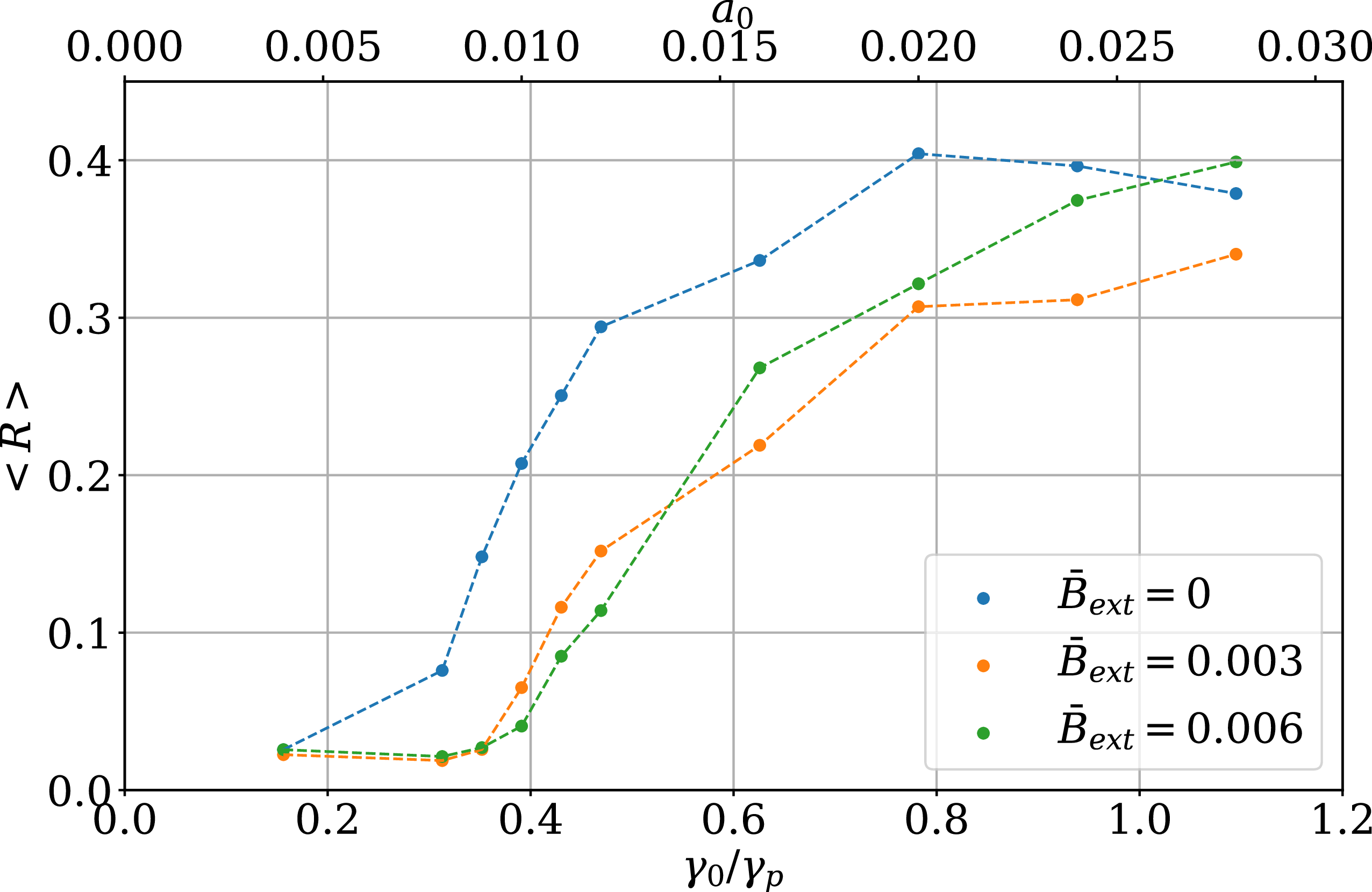
 B¯ext≡ωc/ωp
 ωc
 ωp

 γ0/γp=0.47
 a0=0.012
 R(t)


 γ0/γp=1.11
 a0=0.028
 R(t)


 γ0/γp=1.11
 a0=0.028

 ωpt=20
 ωb2/ωp2=0.014

 x2
 ωpt=20
 ωb2/ωp2=0.014

 ωpt=20
 ωb2/ωp2=0.130

 ωpt=20
 ωb2/ωp2=0.130

 ωpt=20
 ωb2/ωp2=0.130

 ωpt=20
 ωb2/ωp2=0.130

 ωpt=20
 ωb2/ωp2=0.130
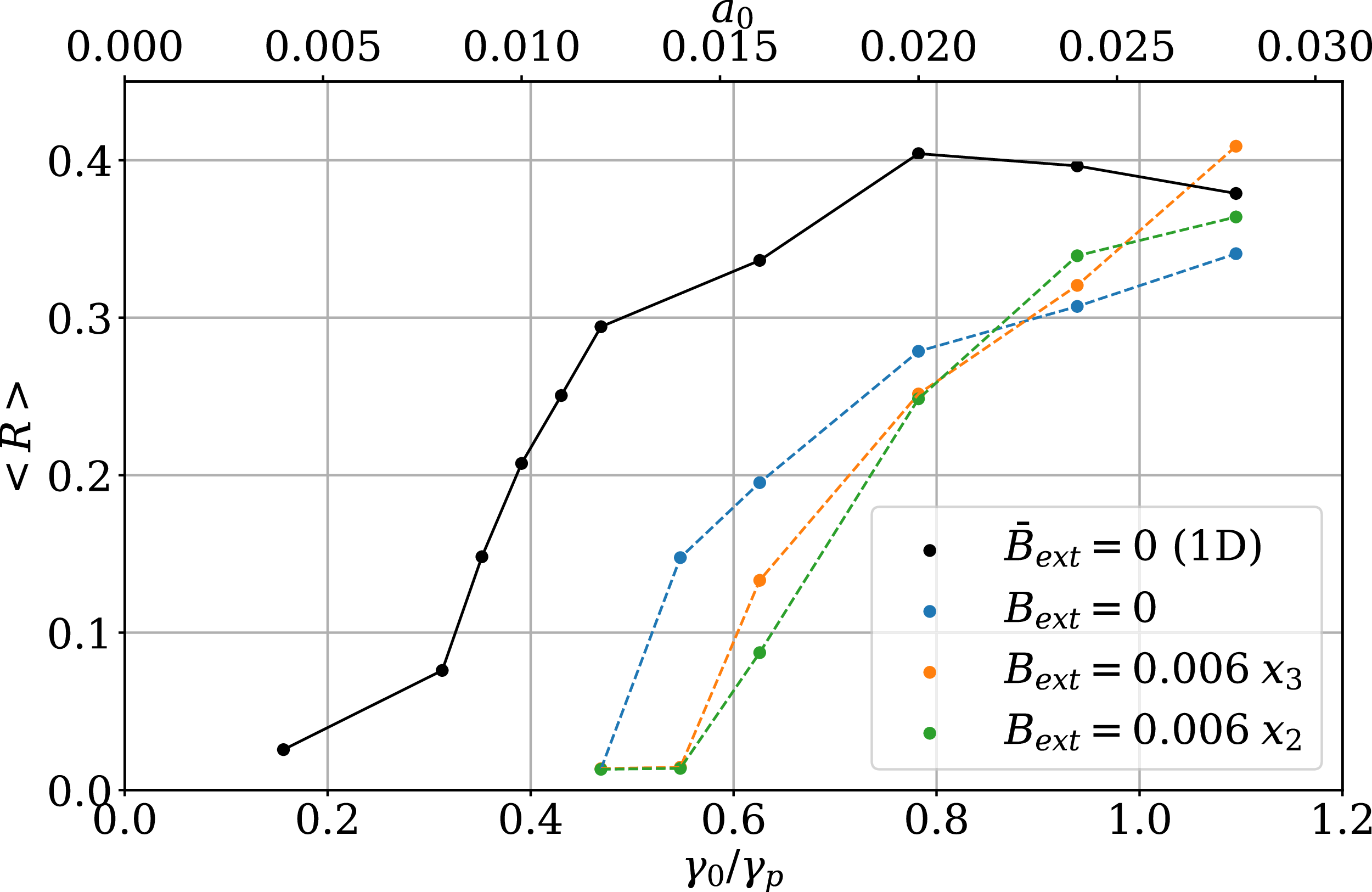

 γ0/γp=1.11

 γ0/γp=1.11

 df(u1)/du1
 u1
 uφ

 Open access

