





1. Introduction
Unsteady flow through porous media plays a fundamental role in numerous natural and engineered systems. In nature, nutrient and gas transport within coral reef skeletons are governed by unsteady currents driven by waves, tides and storm events (Lowe et al. Reference Lowe, Shavit, Falter, Koseff and Monismith2008; Rogers et al. Reference Rogers, Monismith, Koweek, Torres and Dunbar2016). Such hydrodynamic events, as well as density-driven circulation, also drive unsteady flows in coastal aquifers and intertidal zones, producing highly transient flow patterns in permeable sediments and subterranean estuaries (Robinson et al. Reference Robinson, Li and Barry2007; Santos et al. Reference Santos, Eyre and Huettel2012). Frequent storm surges can also cause persistent unsteady conditions in coastal groundwater systems, preventing full recovery between events and inducing repeated perturbations in subsurface water table dynamics (Nordio et al. Reference Nordio, Frederiks, Hingst, Carr, Kirwan, Gedan, Michael and Fagherazzi2023). In subsurface engineering, unsteady porous media flows are central to operations such as carbon capture and storage, where supercritical CO
 $_2$
is injected into deep saline aquifers or depleted hydrocarbon reservoirs. These processes impose a sudden pressure gradient on the porous medium, initiating a transient flow regime (Class et al. Reference Class2009; Sacconi & Mahgerefteh Reference Sacconi and Mahgerefteh2020).
The above examples demonstrate the prevalence of unsteady porous media flows. However, many theoretical and empirical models are based on steady or quasi-steady assumptions, often resulting in a high degree of uncertainty by neglecting the transient, nonlinear and sometimes chaotic nature of the porous media flows. Instead, these established theories of the stationary flows should be viewed as baselines to which the developing flows will eventually evolve into. Subsequently, some prototypical transient flow problems need to be investigated for identification of the asymptotic behaviours that any physically consistent model should reproduce. For instance, oscillatory flows due to a sinusoidal pressure wave have been frequently studied for the flow response to the high and the low-frequency limits (e.g. Zhu & Manhart Reference Zhu and Manhart2016; Unglehrt & Manhart 2022, 2023, 2024), whilst the small- and large-time asymptotics can be determined in the start-up flow under a constant forcing. Once these asymptotics are determined, investigations of the intermediate behaviours should follow to complete the overall picture.
Generally, these fundamental investigations are performed based on idealised porous media geometries to eliminate the geometric uncertainties. Consequently, a monodisperse sphere pack set-up is often preferred to analyse the complex pore-scale flow dynamics in a laboratory-like controlled environment. Examples of such investigations by means of experiments are Dybbs & Edwards (Reference Dybbs and Edwards1984), Horton & Pokrajac (Reference Horton and Pokrajac2009), whilst the numerical counterparts are Maier et al. (Reference Maier, Kroll, Kutsovsky, Davis and Bernard1998), Hill et al. (Reference Hill, Koch and Ladd2001a , Reference Hill, Koch and Laddb ), Hill & Koch (Reference Hill and Koch2002), Nguyen et al. (Reference Nguyen, Kappes, King, Hassan and Ugaz2018), He et al. (Reference He, Apte, Finn and Wood2019). Here, we follow this established approach by numerically investigating start-up flows through monodisperse sphere packs to extract mechanistic insights. Before formulating the specific research questions, we briefly recall the relevant stationary-flow regimes and start-up-flow asymptotics next.
A stationary flow through a porous medium exhibits different flow states, namely: linear (Stokes), steady nonlinear, unsteady nonlinear and turbulence-like chaotic flow (Dybbs & Edwards Reference Dybbs and Edwards1984). These flow states are determined by a dimensionless flow parameter called the Reynolds number (
 $\textit{Re}$
). As mentioned, stationary flows through porous media generally represent the large-time asymptotic of the corresponding unsteady flows. It is therefore expected that weakly transient flows behave similarly to the stationary flows such that they can be described simply according to the instantaneous Reynolds number, given that the dimensional number slowly relaxes towards the steady-state level. In such scenarios, the flow has enough time to adapt to the new equilibrium at each instance. Conversely, under strong acceleration or deceleration, the transient flow is unlikely to depend on the instantaneous Reynolds number.
The linear stationary flow occurs in the very low-Reynolds-number limit
 $\textit{Re} \ll 1$
and is characterised by Darcy's law: a linear dependence of the superficial (volume-averaged) velocity on the driving body force and the counteracting viscous resistance. In this flow regime, if present in the porous media, the fore-aft symmetry in the pore-scale velocity distribution is maintained. At Reynolds numbers of order unity and above, an additional drag force arises from the inertial term in the Navier–Stokes equations, and this nonlinear drag becomes progressively more dominant with increasing
 $\textit{Re}$
. At this stage, the fore-aft symmetry in the pore-scale velocity distribution is broken in the form of flow separations (Sakai & Manhart Reference Sakai and Manhart2020). Despite the increased complexity of the flow features, the nonlinear flow is still steady if the flow Reynolds number is moderate, whilst the flow structures maintain the spatial symmetries in the cross-stream directions imposed by the pore geometries (Hill & Koch Reference Hill and Koch2002; Sakai & Manhart Reference Sakai and Manhart2020). Once the flow Reynolds number reaches values of order
 $10^2$
, the nonlinear flow finally becomes unstable through Hopf bifurcation and eventually transitions to the chaotic flow state at still larger Reynolds numbers.
Generally, the development of wall-bounded start-up flow is also well understood. When a resting fluid is suddenly set into motion by a constant pressure gradient, the resulting velocity field is almost exclusively controlled by the pressure force and, for
 $t \rightarrow 0^+$
, the flow consists of an irrotational outer potential flow and thin Stokes boundary layers adjacent to the solid surfaces. In the context of transient flows through sphere packs, the above implies the coexistence of the potential core flow and thin Stokes boundary layer around the sphere surfaces (Hill et al. Reference Hill, Koch and Ladd2001b
). This boundary layer is initially infinitesimally thin, whose thickness
 $\delta$
grows proportionally to
 $\sqrt {\nu t}$
, where
 $t$
is the elapsed time from the start-up whereas
 $\nu$
is kinematic viscosity of the fluid (Schlichting & Gersten Reference Schlichting and Gersten2017). Based on this boundary-layer theory, the exact thin boundary-layer asymptotics for porous media flow was derived by Johnson et al. (Reference Johnson, Koplik and Dashen1987) in the frequency domain, which can be expressed in the temporal domain by means of inverse Fourier transform (Unglehrt & Manhart Reference Unglehrt and Manhart2023, § B.2). Consequently, the small-time asymptotics of the start-up flow through porous media can be determined.
The growing boundary layers inside porous media eventually fill the entire pores for
 $t \rightarrow \infty$
, and the flow fields converge to the steady-state distributions that represent the large-time asymptotes. In the case of linear start-up flows, the superficial velocity relaxes in an exponential manner towards the steady-state level after the aforementioned small-time asymptotic phase. During this process the flow field behaves like in a quasi-steady state, as it was shown by Hill et al. (Reference Hill, Koch and Ladd2001b
) and Zhu et al. (Reference Zhu, Waluga, Wohlmuth and Manhart2014) who simulated such flows through simple cubic and random arrays and hexagonal close-packed (HCP) spheres, respectively. Furthermore, this late-time exponential relaxation is known to have a characteristic time constant called the energy time scale
 $\tau _{\textit{en}}$
, which makes the relaxations across different porous media similar.
The development of nonlinear transient flows through porous media is much less trivial, and it is known to differ qualitatively from the linear counterpart. For instance, in contrast to the aforementioned exponential relaxation, an overshoot of the superficial velocity briefly before reaching to the steady state was observed in the nonlinear flows through face-centred cubic (FCC) and the HCP sphere packs (Hill & Koch Reference Hill and Koch2002; Zhu & Manhart Reference Zhu and Manhart2016; Sakai & Manhart Reference Sakai and Manhart2020). During the flow development under strong enough acceleration, a sequence of flow structures develops inside the pores, and the structural evolution was found to be identical across steady/unsteady/chaotic nonlinear flow regimes. Furthermore, it was shown that both the velocity overshoot and the pore-scale flow evolution manifest independent of their instantaneous and steady-state Reynolds numbers, and their formation times cannot be described by the normalisation based on the fluid viscosity and a fixed length, such as the sphere diameter (Sakai & Manhart Reference Sakai and Manhart2020). This implies that the quasi-steady-state assumption does not hold in the strongly nonlinear flow since the flow Reynolds number does not play a decisive role. This observation is consistent with the finding of Zhu (Reference Zhu2016) that the deviation from linearity is not a function of the instantaneous Reynolds number in the strongly accelerating porous media flow, which led to an alternative Reynolds number definition based on the Stokes boundary-layer thickness. This newly proposed instantaneous Reynolds number showed a notable improvement over the more conventional fixed-length-based definition to predict nonlinearity onset in a range of porous media, albeit inconclusively. Finally, our more recent contribution (Sakai & Manhart Reference Sakai and Manhart2022) showed that the formation time of the velocity overshoot in the strongly accelerated flow through the HCP sphere pack converges to a constant multiple of the so-called inviscid time scale
 $\tau _{{inv}}$
. The underlying mechanism and whether it applies to other sphere packs are, however, still to be investigated.
In summary, the start-up flows through porous media driven by small pressure gradients can be generally well explained by a combination of the small- and large-time asymptotes. On the other hand, our understanding regarding the development of strongly accelerated start-up flows is much less established. In particular, the onset process of nonlinearity in such flows, emerging in between the small- and large-time limits, has not been explored extensively to date. Besides obvious dynamical interests, addressing this knowledge gap is also crucial for the modelling of the unsteady flow; however, parametrisation of the nonlinear effects is a non-trivial task (Unglehrt & Manhart Reference Unglehrt and Manhart2024).
The above survey leads to the following questions for this study, namely: (i) How general is
 $\tau _{{inv}}$
as a temporal measure to describe strongly accelerated nonlinear porous media flow? For instance, can it be used to describe other nonlinear flow through different sphere pack geometries? (ii) Given that the velocity overshoot is a nonlinear phenomenon and timed by
 $\tau _{{inv}}$
, does this time scale generally control the nonlinearity onset? If so, what is the underlying mechanism? (iii) Which of the changes in the flow field are associated with
 $\tau _{{inv}}?$
Consequently, we define the following objectives and the corresponding structure of this paper. We analyse the high-fidelity direct numerical simulation (DNS) dataset of flow through the HCP spheres from Sakai & Manhart (Reference Sakai and Manhart2020), as well as two additional DNS datasets of flow through FCC and body-centred cubic (BCC) sphere packs. After presenting the simulation approach and the properties of the datasets, we perform a dimensional analysis to determine the governing time scales of the start-up flow through sphere packs. Then, based on the boundary-layer theory and an order-of-magnitude analysis, we show that the onset of nonlinearity emerging from the sphere surfaces should be timed by
 $\tau _{{inv}}$
. The validity of the above conjecture is then demonstrated based on the DNS datasets. In the end, by means of scaling arguments, it becomes evident that the employed boundary-layer theory in the start-up flow can consistently describe the considered transient flows through sphere packs, not only qualitatively but also quantitatively.
2. Numerical methods
The flow solver MGLET was used to generate all three DNS datasets being considered in this study. The code solves the following incompressible Navier–Stokes equations:
 \begin{align} \boldsymbol{\nabla }\boldsymbol{\cdot }\boldsymbol{u} &= 0, \\[-12pt]\nonumber \end{align}
 \begin{align} \partial _t \boldsymbol{u} + \boldsymbol{\nabla } \boldsymbol{\cdot }(\boldsymbol{u} \otimes \boldsymbol{u}) &= - \frac {1}{\rho } \boldsymbol{\nabla }\!p + \nu \Delta \boldsymbol{u} -\frac {1}{\rho } \boldsymbol{\nabla }\! \left \langle p\right \rangle _{\textit{i}} . \end{align}
Here the velocity vector
 $\boldsymbol{u} = [u, v, w]$
corresponds to the Cartesian spatial directions
 $\boldsymbol{x} = [x,y,z]$
,
 $p$
is the pore-scale pressure variations and
 $\boldsymbol{\nabla }\!\langle p\rangle _{\textit{i}} = [\vert \boldsymbol{\nabla }\!\langle p\rangle _{\textit{i}}\vert , 0, 0]$
is the prescribed constant intrinsic pressure gradient driving the flow in the
 $x$
direction. The parameters
 $\rho$
and
 $\nu$
are the fluid density and kinematic viscosity, respectively, which are also constant in space and time. For a constant-density incompressible fluid under uniform gravity, the gravitational body force is conservative and can be absorbed into the definition of the pressure as a hydrostatic contribution (cf. modified pressure described in Kundu et al. (Reference Kundu, Cohen and Dowling2015, pp. 119, 280)), irrespective of the orientation of the coordinate system. Therefore, the present
 $p$
represents the dynamic pressure relative to the hydrostatic contribution. Since the present simulations contain no density variation or free surface, there is no separate buoyancy term in (2.2).
As detailed in the subsequent section, all of the present simulations are performed in triply periodic domains, which implies that
 $p$
is the spatially periodic pore-scale pressure variation. Accordingly, the total pressure field
 $\mathcal{P}$
is decomposed as
 $\mathcal{P} = p + \boldsymbol{\nabla }\!\langle p\rangle _{\textit{i}} \boldsymbol{\cdot }\boldsymbol{x}$
. Since the
 $ \boldsymbol{\nabla }\!\langle p\rangle _{\textit{i}}$
vector is independent of space and time,
 $\boldsymbol{\nabla }\mathcal{P} = \boldsymbol{\nabla }\!p + \boldsymbol{\nabla }\!\langle p\rangle _{\textit{i}}$
. Thus, (2.2) is the periodic formulation for the pressure variations
 $p$
under the imposed macroscopic pressure gradient. In relation to the direction of the applied macroscopic pressure gradient, in the rest of this paper we refer to the direction
 $x$
as the streamwise direction, whilst
 $y$
and
 $z$
are referred to as the cross-flow directions (also, cf. figure 1).
Since we study start-up flows, the use of the incompressible form of the Navier–Stokes equations and the constant macroscopic pressure gradient need justification beyond the traditional Mach number estimation. In essence, one can only assume the pressure gradient to be constant after the initial pressure waves have travelled much greater distance than the computational domain extent within the time frame being considered. In Appendix C we provide an order-of-magnitude estimate of the pressure wave travel distances in terms of the fluid properties and the relevant dimensionless numbers.
The above velocities are stored in a staggered arrangement and discretised in space by the second-order central finite-volume method, which is combined with a second-order mass-conserving immersed boundary method (Peller et al. Reference Peller, Duc, Tremblay and Manhart2006; Peller Reference Peller2010; Sakai & Manhart Reference Sakai and Manhart2020) to handle arbitrary-shaped domains. An explicit third-order low-storage Runge–Kutta method (Williamson Reference Williamson1980) integrates the governing equations in time, whilst the projection method of Chorin (Reference Chorin1968) decouples the velocity and pressure computations. For every Runge–Kutta substep, a Poisson equation is solved for
 $p$
by means of a strongly implicit procedure (SIP) solver (Stone Reference Stone1968), which has been recently optimised for the modern SIMD processors. The code is written in Fortran and parallelised by means of the message passing interface (MPI), which scales efficiently up to parallel processes of order
 $10^5$
on the modern massively parallel systems (Sakai et al. Reference Sakai, Mendez, Strandenes, Ohlerich, Pasichnyk, Allalen and Manhart2019).
3. Direct numerical simulation datasets
In this contribution we consider three different close-pack arrangements of uniform spheres, namely: HCP, FCC and BCC sphere packs (Conway & Sloane Reference Conway and Sloane1999), shown in figure 1. These sphere packs are characterised by the sphere diameter
 $d$
and the porosity
 $\epsilon$
(cf. table 1).
Geometric properties of the hexagonal close-packed, FCC and BCC sphere packs.

Table 1. Long description
A table comparing geometric properties of hexagonal close-packed, FCC, and BCC sphere packs. The table has four rows and five columns. Column headers are Porosity, Permeability, Weighted pore-volume-to-surface ratio, Static viscous tortuosity, and High-frequency limit of the dynamic tortuosity. Row labels are HCP, FCC, and BCC. Row 1: HCP, Porosity 0.259, Permeability 1.73 times 10 to the power of negative 4 a, Weighted pore-volume-to-surface ratio 5.9 times 10 to the power of negative 2 c, Static viscous tortuosity 2.66 d, High-frequency limit of the dynamic tortuosity 1.62 c. Row 2: FCC, Porosity 0.259, Permeability 1.73 times 10 to the power of negative 4, Weighted pore-volume-to-surface ratio 6.2 times 10 to the power of negative 2 b, Static viscous tortuosity 2.65, High-frequency limit of the dynamic tortuosity 1.61 b. Row 3: BCC, Porosity 0.320, Permeability 5.16 times 10 to the power of negative 4, Weighted pore-volume-to-surface ratio 9.6 times 10 to the power of negative 2 b, Static viscous tortuosity 2.22, High-frequency limit of the dynamic tortuosity 1.47 b.
 $\,{}^{a}$
Sakai & Manhart (Reference Sakai and Manhart2020),
 $\,{}^{b}$
Chapman & Higdon (Reference Chapman and Higdon1992),
 $\,{}^{c}$
Unglehrt & Manhart (Reference Unglehrt and Manhart2023),
 $\,{}^{d}$
Zhu & Manhart (Reference Zhu and Manhart2016).
The three sphere pack geometries being considered in this study. To highlight the pore-scale flow features, the magnitude of an instantaneous velocity field is included, where red and blue colours indicate high and low magnitudes, respectively. The cut planes correspond to a symmetry plane for each sphere pack: HCP,
 $\sqrt {3}y/3 + \sqrt {6}z/3=0$
; FCC,
 $y -z= 0$
; BCC,
 $z=d/2$
. Green shaded planes correspond to the cross-stream planes for examining the pore-scale flow features: HCP,
 $x=d$
; FCC,
 $x=\sqrt {2}d/2$
; BCC,
 $x=2d/\sqrt {3}$
.

The triply periodic boundary conditions are applied at each end of the numerical domains, which have the spatial extents of
 $[L_x, L_y, L_z]$
in the Cartesian coordinate directions. Note that whilst we simulate a single unit cell for the FCC and BCC configurations, the domain extent of the HCP case is doubled in the
 $x$
direction in order to accommodate the symmetry breaking in the streamwise direction that appears when the flow state is highly chaotic (Sakai & Manhart Reference Sakai and Manhart2020).
All three sphere pack geometries contain nominally touching spheres, and all were treated consistently by the same ghost-cell immersed-boundary-method discretisation. No artificial overlap, separation gap, or connector was introduced. As a consequence of the Cartesian discretisation, subgrid passages at touching contacts are blocked once the local separation falls below the immersed-boundary-method resolution limit, so the exact contact region does not act as an artificially open fluid throat.
In all the simulation cases presented, initially resting fluid (i.e.
 $\boldsymbol{u}(\boldsymbol{x},0)=0$
) in the triply periodic domain is accelerated by a constant intrinsic pressure gradient
 $ \boldsymbol{\nabla }\!\langle p\rangle _{\textit{i}}$
until a steady state is established. Consequently, this formulation isolates pore-scale start-up dynamics under an established macroscopic pressure gradient, and does not include entrance effects or the development of the pressure gradient through a finite porous media sample.
The resulting accelerating porous media flow is characterised by the so-called Hagen number, i.e.
 \begin{equation} {\textit {Hg}} = \frac {\left \vert \boldsymbol{\nabla }\!\left \langle p\right \rangle _{\textit{i}}\right \vert d^3}{\rho \nu ^2}, \end{equation}
whilst the (statistically) steady-state Reynolds number (
 $\textit{Re}_{\textit{steady}}$
) is often used to describe the steady-state flow, which is simply a function of
 $\textit {Hg}$
. Note that by normalising with
 $\rho$
,
 $d$
and
 $\vert \boldsymbol{\nabla }\!\langle p\rangle _{\textit{i}}\vert$
, the governing equations (2.2) can be expressed in the following dimensionless form such that the flow field depends solely on
 $\textit {Hg}$
:
 \begin{align} \hat { \boldsymbol{\nabla }} \boldsymbol{\cdot }\hat {\boldsymbol{u}} &= 0, \\[-12pt]\nonumber \end{align}
 \begin{align} \hat {\partial _t} \hat {\boldsymbol{u}} + \hat {\boldsymbol{\nabla }} \boldsymbol{\cdot }(\hat {\boldsymbol{u}} \otimes \hat {\boldsymbol{u}}) &= -\hat { \boldsymbol{\nabla }}\! \hat {p} + \frac {1}{\sqrt {{\textit {Hg}}}} \hat {\Delta } \hat {\boldsymbol{u}} + \boldsymbol{e}_x. \end{align}
Here
 $\hat {(*)}$
represents non-dimensionalised variables (i.e.
 $\hat {\boldsymbol{u}} = \boldsymbol{u}/\sqrt {(\vert \boldsymbol{\nabla }\!\langle p\rangle _{\textit{i}}\vert d)/\rho }$
,
 $\hat {p} = p/(\vert \boldsymbol{\nabla }\!\langle p\rangle _{\textit{i}}\vert d)$
,
 $\hat {t} = t/\sqrt {\rho d/\vert \boldsymbol{\nabla }\!\langle p\rangle _{\textit{i}}\vert }= t/\tau _{{inv}}$
) and operators. The governing parameter
 $\textit {Hg}$
can be seen as the ratio of the intrinsic pressure gradient to the viscous forces, and has been referred to as a pressure-gradient-based Reynolds number in other works (e.g. Schlichting & Gersten Reference Schlichting and Gersten2017, p. 416).
To ensure the comparability to existing steady flow studies, we define the aforementioned Reynolds number as follows. This Reynolds number is based on the superficial (volume-averaged) streamwise velocity, i.e.
 \begin{equation} \left \langle u\right \rangle _{\textit{s}} = \frac {1}{V}\int _{V_{\!{f}}} u(\boldsymbol{x},t)\,\mathrm{d}V , \end{equation}
where
 $V_{\!{f}}$
is the fluid volume, whilst
 $V = L_x\,L_y\,L_z$
includes the volume of spheres as well in which the velocity is set at zero. Note that the corresponding intrinsic (fluid-volume-averaged) velocity can be determined by using porosity as
 $\langle u\rangle _{\textit{i}} = \langle u\rangle _{\textit{s}}/\epsilon$
. The corresponding Reynolds number is defined as
 \begin{equation} \textit{Re}_{\textit{steady}} = \frac {\overline {\left \langle u\right \rangle _{\textit{s}}}d}{\nu } , \end{equation}
where
 $\overline {(*)}$
represents a (statistically) steady state. Alternatively, the Reynolds number definition based on the hydraulic diameter (
 $\textit{Re}_{\textit{H}}$
) is also commonly used, which is particularly useful to compare porous media with different porosity as in this study. This Reynolds number is related to
 $\textit{Re}_{\textit{steady}}$
in the following manner (Wood et al. Reference Wood, He and Apte2020):
 \begin{equation} \textit{Re}_{\textit{H}} = \frac {\textit{Re}_{\textit{steady}}}{1-\epsilon }. \end{equation}
Finally, a set of volume-averaged quantities, such as the superficial velocity and energy, were sampled at least every 40 time steps from the start-up on-the-fly for each simulation, in addition to the velocity and pressure distributions on a cross-flow plane at the full spatial resolution. Additionally, a series of snapshots of the complete flow field were saved for some key simulation cases.
Numerical and physical parameters of the HCP simulations examined in this study. The entries on the second column correspond to the case names introduced in Sakai & Manhart (Reference Sakai and Manhart2020) and referred to in Unglehrt & Manhart (Reference Unglehrt and Manhart2023), whose suffixes describe the flow state as linear (L), steady nonlinear (SNL), unsteady nonlinear (UNL) and turbulent (T).

Table 2. Long description
A table with 11 rows and 7 columns comparing numerical and physical parameters of HCP simulations. Column headers are: CASE, CASE in SM20, Hg, Re_steady, Re_H, Colour/marker, d/Δx. Row labels are: H1, H2, H3, H4, H5, H6, H7, H8, H9, H10, H11. Row 1: H1, L6, 6.5 x 10^3, 1, 1.35, +, 160. Row 2: H2, SNL1, 6.5 x 10^4, 10, 13.5, +, 160. Row 3: H3, SNL2, 3.3 x 10^5, 36, 48.6, o, 160. Row 4: H4, SNL3, 4.9 x 10^5, 48, 64.9, □, 160. Row 5: H5, SNL4, 6.5 x 10^5, 59, 79.7, △, 320. Row 6: H6, UNL1, 1.3 x 10^6, 91, 123, +, 320. Row 7: H7, UNL2, 2.6 x 10^6, 138, 186, o, 320. Row 8: H8, T1, 5.2 x 10^6, 209, 282, □, 320. Row 9: H9, T2, 7.8 x 10^6, 254, 343, △, 320. Row 10: H10, T3, 1.0 x 10^7, 305, 412, □, 320. Row 11: H11, T4, 1.3 x 10^7, 347, 469, △, 320.
3.1. Hexagonal close-packing
The results of this high-fidelity DNS dataset consisting of 16 cases were first published in Sakai & Manhart (Reference Sakai and Manhart2020). The HCP sphere pack geometry is defined by the sphere geometric centres, as
 \begin{align} \begin{bmatrix} x_{\textit{c}} \\[3pt] y_{\textit{c}} \\[3pt] z_{\textit{c}} \\ \end{bmatrix} = \begin{bmatrix} 2i + ((j+k) \mod 2) \\[11pt] \sqrt {3}\left[j+\dfrac {1}{3}(k \mod 2)\right]\\[11pt] \dfrac {2\sqrt {6}}{3}k \end{bmatrix} \dfrac {d}{2} ,\end{align}
where
 $i$
,
 $j$
,
 $k=0 \ldots n$
are the sphere indices in the
 $x$
,
 $y$
and
 $z$
direction, respectively. For this study, its subset of 11 cases are evaluated (cf. table 2). The porosity of this HCP sphere pack is at the close-pack limit of
 $\epsilon = 1-( {\pi }/({3\sqrt {2}))} \approx 0.259$
, which means all the spheres are in contact with their 12 neighbours. The spatial extents of the numerical domain are
 $[L_x, L_y, L_z]/d = [2, \sqrt {3}, (( {2\sqrt {6}})/{3})]$
. This sphere pack geometry with respect to the considered primary flow direction features a split-and-merging pattern of alternating smaller and larger pores, which is highlighted in figure 1(a) by means of a symmetry-plane cutout. Due to this geometric constraint, the flow is accelerated significantly through the smaller pores, before it reduces the velocity magnitude in the subsequent larger cavities. Once
 $\textit {Hg}$
becomes sufficiently high, the primary flow starts to separate from the sphere surface behind the sphere contact points inside the larger pores (cf. Sakai & Manhart Reference Sakai and Manhart2020 and also the velocity magnitude distribution in figure 1
a).
The
 $\textit {Hg}$
range being covered by this dataset is
 $3.25 \times 10^{-3} \leq {\textit {Hg}} \leq 1.3 \times 10^{7}$
, spanning over linear, steady nonlinear, unsteady nonlinear and turbulent flow regimes. We employed equidistant grid point distributions in the
 $x$
,
 $y$
and
 $z$
directions, with
 $160$
finite-volume cells per diameter up to
 ${\textit {Hg}}=4.9\times 10^{5}$
and
 $320$
points per diameter between
 $6.5 \times 10^{5} \leq {\textit {Hg}} \leq 1.3 \times 10^{7}$
. The corresponding grid convergence study was carried out and presented in Sakai & Manhart (Reference Sakai and Manhart2020, figure 3) and Unglehrt & Manhart (Reference Unglehrt and Manhart2022, figure 2). This highly adequate grid resolution was adopted to resolve the very thin potential-flow-type boundary layers forming on the sphere surface when the flow is suddenly accelerated from rest. For adequate temporal accuracy, the maximum Courant--Friedrichs--Lewy (CFL) number was kept below 0.16.
Numerical and physical parameters of the FCC (F cases) and the BCC (B cases) simulations. The entries in the second column correspond to the flow state as linear (L), steady nonlinear (SNL), unsteady nonlinear (UNL) and turbulent (T).

Table 3. Long description
A table with 11 rows and 6 columns comparing numerical and physical parameters of FCC and BCC simulations. The columns are labeled CASE, Flow state, Hg, Re_steady, Re_H, Colour/marker, and d/Δx. The table includes data for FCC (F cases) and BCC (B cases) simulations, with flow states categorized as linear (L), steady nonlinear (SNL), unsteady nonlinear (UNL), and turbulent (T). Each row provides specific values for Hg, Re_steady, Re_H, Colour/marker, and d/Δx for different cases. Notable trends include variations in Hg and Re_H values across different flow states and cases.
3.2. Face-centred cubic packing
This dataset of the flow though the FCC sphere pack consists of 11 DNS results, which covers
 $5.6 \times 10^{1} \leq {\textit {Hg}} \leq 1.2 \times 10^7$
(cf. table 3). The spatial extents of the numerical domain are
 $[L_x, L_y, L_z]/d = [\sqrt {2}, \sqrt {2}, \sqrt {2}]$
. The porosity of the sphere pack is at the close-pack limit of
 $\epsilon \approx 0.259$
, which is identical to that of the HCP configuration. The split-and-merging pattern mentioned for the HCP sphere pack is also featured in this geometry, meaning the fluid inside one larger pore subsequently flows into four smaller pores before merging in the following larger pore. Previously, it was reported that a small wake-like reverse flow region forms directly behind one of the spheres enclosing the larger pore space (Hill et al. Reference Hill, Koch and Ladd2001a
; He et al. Reference He, Apte, Finn and Wood2019), indicating the existence of significant flow separations under a strong inertial influence. Such geometric and flow feature are visualised in figure 1(b).
We employed equidistant grid point distributions in the
 $x$
,
 $y$
and
 $z$
directions, with
 $158$
finite-volume cells per diameter in the cases up to
 ${\textit {Hg}} = 2.3 \times 10^6$
and
 $316$
cells per diameter between
 ${\textit {Hg}} = 4.6 \times 10^{6}$
and
 $1.2 \times 10^{7}$
. Note that this grid resolution is significantly higher than the required resolution reported in He et al. (Reference He, Apte, Finn and Wood2019) to achieve a grid convergence of the mean flow as well as second-order statistics in their FCC porous media flow up to
 $\textit{Re}_{\textit{steady}}=370$
. For adequate temporal accuracy, the maximum CFL number was kept below 0.31. The simulation results were validated against the data available in the literature and are summarised in Appendix A.1. Moreover, the flow state corresponding to each case was determined based on the geometric symmetries of the pore-scale flow, and also summarised in Appendix A.1. Consequently, we categorise that F1 belongs to the linear flow regime, cases F2–F5 are in the steady nonlinear regime, F6 belongs to the unsteady nonlinear flow and F7–F11 fall into the turbulent/chaotic flow category.
3.3. Body-centred cubic packing
This dataset of the flow through a BCC sphere pack consists of 11 DNS results (cf. table 3). The range of
 $\textit {Hg}$
covered by this dataset is
 $2 \times 10^{2} \leq {\textit {Hg}} \leq 4 \times 10^{6}$
. The spatial extents of the numerical domain are
 $[L_x, L_y, L_z]/d = [{2}/{\sqrt {3}}, {2}/{\sqrt {3}}, {2}/{\sqrt {3}}]$
. The porosity of this geometry is at
 $\epsilon \approx 0.32$
, which is approximately
 $23\,\,\%$
higher than the other two configurations. This higher porosity is readily visible in figure 1(c), where large, straight unobstructed pore channels pointing in the streamwise direction are featured on four sides (i.e. top, bottom, left and right) of the central sphere. A grid resolution of
 $166$
finite-volume cells per diameter is adopted for the cases up to
 ${\textit {Hg}} = 8 \times 10^5$
, whereas
 $332$
cells per diameter resolution is used for the cases between
 ${\textit {Hg}} = 1.6 \times 10^6$
and
 $4 \times 10^6$
. The maximum CFL number was kept below 0.35. As for FCC spheres, the simulation results were compared with the data available in the literature and are summarised in Appendix A.2.
As for HCP and FCC spheres, the flow state corresponding to each case was determined based on the geometric symmetries of the pore-scale flow as summarised in Appendix A.2. Accordingly, we categorise B1 to be in the linear flow regime, cases B2–B6 are in the steady nonlinear flow regime, B7 is in the unsteady nonlinear regime and cases B8–B11 are in the turbulent/chaotic flow regime.
4. Time scales in transient flow
Here, we discuss the evolution of the start-up flow with a special focus on the governing time scales of different physical processes. First, we perform a dimensional analysis to identify two time scales that are relevant in the accelerating flow through porous media. Then, based on the identified time scales, we perform an a-priori order-of-magnitude analysis, leading to a hypothesis that one of the two time scales controls onset of nonlinearity emerging in the pore space. Finally, the hypothesis is tested against the DNS data.
4.1. Dimensional analysis
We assume that the following fundamental parameters describe the start-up flow field within the porous media
 $\boldsymbol{u}(\boldsymbol{x},t)$
: the fluid density
 $\rho$
and kinematic viscosity
 $\nu$
, the sphere diameter
 $d$
, the intrinsic pressure gradient driving the flow
 $\vert \boldsymbol{\nabla }\!\langle p\rangle _{\textit{i}}\vert$
and the elapsed time
 $t$
. Porosity
 $\epsilon$
and the permeability
 $K$
of the porous media are left out, since they are pure functions of the geometry and remained constant for each sphere pack.
Depending on which dimensionally independent variables are selected as the repeating variables in the Buckingham–Pi sense, different but equivalent sets of dimensionless groups can be formed. For instance, with
 $d$
,
 $\vert \boldsymbol{\nabla }\!\langle p\rangle _{\textit{i}}\vert$
and
 $\nu$
, the following functional relation of the corresponding dimensionless groups can be formed:
 \begin{equation} \frac {u\, d}{\nu } = \textit{Re} = \frac {u\, \tau _{v\textit{isc}}}{d} = \varPhi \!\left ({\textit {Hg}},\; \frac {t}{\tau _{v\textit{isc}}} \right )\!. \end{equation}
Here
 $\varPhi$
is an arbitrary function, whereas the normalisation factor
 $\tau _{v\textit{isc}}$
is a viscous time scale:
 \begin{equation} \tau _{v\textit{isc}}=\frac {d^2}{\nu }. \end{equation}
This time scale controls the flow evolution when it is predominantly influenced by viscosity
 $\nu$
– one of the repeating variables – and represents the required time to reach an equilibrium by molecular diffusion. Moreover, since
 $K$
and
 $\epsilon$
are constant, the aforementioned energy time scale
 $\tau _{\textit{en}}$
can be expressed in terms of
 $\tau _{v\textit{isc}}$
as
 \begin{equation} \tau _{\textit{en}}=\frac {\alpha _0}{\epsilon } \left ( \frac {K}{d^2} \right ) \tau _{v\textit{isc}}, \end{equation}
where
 $\alpha _0$
is static viscous tortuosity, which is a purely geometrical-hydrodynamic property of the porous structure (cf. table 1). This tortuosity
 $\alpha _0$
is the low-frequency ratio by which the actual kinetic energy of fluid in a porous medium exceeds the kinetic energy computed from the superficial velocity, due to the non-uniform pore-scale velocity field created by viscous flow (Zhu et al. Reference Zhu, Waluga, Wohlmuth and Manhart2014).
On the other hand, if we select
 $\rho$
instead of
 $\nu$
as a repeating variable – corresponding to the situations where the viscosity effect is not predominant – the following functional relation can be found:
 \begin{equation} \frac {u\, \tau _{{inv}}}{d} = \varPsi \!\left ({\textit {Hg}},\; \frac {t}{\tau _{{inv}}} \right )\!. \end{equation}
Here
 $\varPsi$
is another arbitrary function, whilst
 $\tau _{{inv}}$
is an inviscid time scale:
 \begin{equation} \tau _{{inv}}=\left (\frac {\rho d}{\left \vert \boldsymbol{\nabla }\!\left \langle p\right \rangle _{\textit{i}}\right \vert }\right )^{\frac {1}{2}}\!. \end{equation}
The mechanistic implication of the inviscid time scale at the pore scale will be analysed in the following section. Moreover, the square of the ratio of the viscous to the inviscid time scale forms the aforementioned Hagen number, viz.
 \begin{equation} \left (\frac {\tau _{v\textit{isc}}}{\tau _{{inv}}}\right )^2 = {\textit {Hg}} , \end{equation}
which can also be seen as the ratio of the intrinsic pressure gradient to the viscous forces. Note that
 $\textit {Hg}$
emerges as a governing dimensionless parameter independent of the repeating variable choices, whilst
 $\textit{Re}$
and
 $\textit{Re}_{\textit{steady}}$
are unique functions of
 $\textit {Hg}$
and dimensionless time.
4.2. Onset of nonlinearity in the boundary layer
Next, we analyse the Stokes boundary layer developing on the sphere surfaces in the flow through the porous medium. Immediately after start-up, the pore-scale flow is not yet influenced by viscous diffusion beyond thin Stokes layers adjacent to the solid surfaces. Hence, in the pore interior the leading-order flow is irrotational and can be approximated by a potential flow, while viscous effects remain confined to the boundary layers. With increasing time, the boundary layers propagate into the pore interior due to viscous diffusion (cf. figure 2 for a linear flow example). Since the nonlinearity of the flow generally arises from the convective term in the governing equations, it is initially at zero within the boundary layer and builds up with the flow velocity.
Schematic of linear transient flow development from a potential flow for
 $t \rightarrow 0^+$
over a potential core flow with growing Stokes boundary layers (blue shaded regions) for small
 $t\gt 0$
towards a fully developed Stokes flow for
 $t\to \infty$
. The simulations start from rest,
 $\boldsymbol{u}(\boldsymbol{x},0)=0$
, and for
 $t \rightarrow 0^+$
, the flow develops an irrotational core flow with thin Stokes boundary layers at the solid surfaces.

In local coordinates (
 $s$
,
 $n$
) tangential and normal to the sphere surface, the boundary layers developing on the sphere surfaces should satisfy the following unsteady laminar boundary-layer momentum balance (Schlichting & Gersten Reference Schlichting and Gersten2017):
 \begin{equation} \frac {\partial u_s}{\partial t} + u_s\frac {\partial u_s}{\partial s} + u_n\frac {\partial u_s}{\partial n} = -\frac {1}{\rho }\frac {\partial p}{\partial s} + \nu \frac {\partial ^2 u_s}{\partial n^2} - \frac { \boldsymbol{\nabla }\langle p\rangle _{\textit{i}}}{\rho }.\end{equation}
Here
 $u_s$
and
 $u_n$
are the tangential and surface-normal velocity components, respectively. In the following, we perform an order-of-magnitude estimation of this equation with a focus on high-
 $\textit {Hg}$
flows such that
 $\tau _{{inv}} \ll \tau _{v\textit{isc}}$
(cf. (4.6)).
In the following scaling estimates,
 $A\sim B$
denotes equality at the level of characteristic scaling, i.e.
 $A/B$
is bounded above and below by non-zero dimensionless constants independent of the scaling variables retained in the estimate. Numerical prefactors, signs and geometry-dependent coefficients are not determined.
Using these assumptions and the characteristic scales
 $U$
(tangential velocity),
 $L$
(tangential length),
 $\delta$
(normal length, boundary-layer thickness),
 $P$
(pressure) and
 $T$
(time), (4.7) can be estimated in table 4.
Order-of-magnitude estimates of the terms in the unsteady laminar boundary-layer momentum equation (4.7) in terms of characteristic scales.

Table 4. Long description
A table with two columns and five rows. The first column is labeled ‘Term’ and the second column is labeled ‘Characteristic magnitude’. Row 1: Term, ∂u_s/∂t; Characteristic magnitude, U/T. Row 2: Term, u_s∂u_s/∂s + u_n∂u_s/∂n; Characteristic magnitude, U^2/L. Row 3: Term, ρ^(-1)∂p/∂s; Characteristic magnitude, P/(ρL). Row 4: Term, ∂^2u_s/∂n^2; Characteristic magnitude, νU/δ^2. Row 5: Term, |∇(p)|/ρ; Characteristic magnitude, |∇(p)|/ρ.
Here, ‘characteristic magnitude’ means that numerical prefactors depending on the local geometry and on the precise boundary-layer profile are not retained. Note that the two convective contributions
 $u_s\partial u_s/\partial s$
and
 $u_n\partial u_s/\partial n$
in (4.7) are grouped into a single convective term, based on the boundary-layer scaling and continuity
 $u_n/U \sim \delta /L$
.
Next, we estimate the characteristic scales as follows. During the initial acceleration, the characteristic time
 $T$
can be equated to the elapsed time
 $t$
since the start (i.e.
 $T \sim t$
). On the other hand, the characteristic velocity scale can be estimated from the accelerating potential-flow solution as
 $U \sim \rho ^{-1} |\boldsymbol{\nabla }\!\langle p\rangle _{\textit{i}}|\, t$
, and the pressure scale is determined by the macroscopic pressure gradient (
 $P \sim |\boldsymbol{\nabla }\!\langle p\rangle _{\textit{i}}|\,d$
). Note that the boundary-layer thickness is taken proportional to the diffusion length (
 $\delta \sim \sqrt {\nu t}$
), whereas the tangential length scale in the other terms is taken as the sphere diameter (
 $L \sim d$
). The former estimation is deduced from the high-
 $\textit {Hg}$
flow assumption, where the viscous diffusion of momentum is confined within very thin boundary layers on the sphere surfaces. By inserting these estimates and dividing by
 $\vert \boldsymbol{\nabla }\!\langle p\rangle _{\textit{i}}\vert /\rho$
, we obtain the dimensionless order-of-magnitude estimation, as summarised in table 5.
Dimensionless order-of-magnitude estimates for the high-
 $\textit {Hg}$
start-up regime, normalised by
 $\left\vert\boldsymbol{\nabla }\!\langle p\rangle _{\textit{i}} \right\vert/\rho$
.

Table 5. Long description
A table with two columns and five rows. The first column is labeled ‘Term’ and the second column is labeled ‘Characteristic magnitude divided by |∇<p>|/ρ’. The rows list different terms and their corresponding characteristic magnitudes. Row 1: Term, ∂u_s/∂t; Characteristic magnitude divided by |∇<p>|/ρ, 1. Row 2: Term, u_s∂u_s/∂s + u_n∂u_s/∂n; Characteristic magnitude divided by |∇<p>|/ρ, (t/τ_inv)^2. Row 3: Term, ρ^(-1)∂p/∂s; Characteristic magnitude divided by |∇<p>|/ρ, 1. Row 4: Term, ν∂^2u_s/∂n^2; Characteristic magnitude divided by |∇<p>|/ρ, 1. Row 5: Term, |∇<p>|/ρ; Characteristic magnitude divided by |∇<p>|/ρ, 1.
Hence, the local-acceleration, pressure-gradient, viscous-diffusion and driving-force terms are all of order unity, whereas the convective term is of order
 $ ( {t}/{\tau _{{inv}}} )^2$
. This estimate indicates that the convective contribution is asymptotically smaller than the leading-order terms for
 $t\ll \tau _{{inv}}$
, but can become comparable to them when
 $t$
reaches times of order
 $\tau _{{inv}}$
, signalling the onset of nonlinear inertial effects.
Conversely, if
 $\textit {Hg}$
is sufficiently low, the boundary layer fills the entire pore space before the inviscid nonlinear time scale is reached. In such a scenario, the velocity scale
 $U$
can no longer be represented by a potential-flow solution, but rather by the steady-state velocity according to Darcy's law (i.e.
 $U \sim d^2 \rho ^{-1} \nu ^{-1} | \boldsymbol{\nabla }\!\langle p\rangle _{\textit{i}}|$
). Correspondingly, the length scale for the viscous-diffusion term
 $\delta$
should be of order
 $d$
. Then we obtain the following order-of-magnitude estimate (table 6).
Dimensionless order-of-magnitude estimates for the low-
 $\textit {Hg}$
viscous regime, normalised by
 $\left\vert\boldsymbol{\nabla }\!\langle p\rangle _{\textit{i}}\right\vert/\rho$
.

Table 6. Long description
A table with two columns and six rows. The first column is labeled ‘Term’ and the second column is labeled ‘Characteristic magnitude divided by |∇(p)|/ρ’. The rows are as follows: Row 1: Term, ∂u_s/∂t; Characteristic magnitude divided by |∇(p)|/ρ, τ_visc/t. Row 2: Term, u_s∂u_s/∂s + u_n∂u_s/∂n; Characteristic magnitude divided by |∇(p)|/ρ, Hg. Row 3: Term, ρ^(-1)∂p/∂s; Characteristic magnitude divided by |∇(p)|/ρ, 1. Row 4: Term, ν∂^2u_s/∂n^2; Characteristic magnitude divided by |∇(p)|/ρ, 1. Row 5: Term, |∇(p)|/ρ; Characteristic magnitude divided by |∇(p)|/ρ, 1.
As expected, the local-acceleration term has become time-dependent and diminishes at the large-time limit (
 $t \rightarrow \infty$
). The timing of the saturation is controlled by
 $\tau _{v\textit{isc}}$
. Meanwhile, the nonlinearity that is represented by the convective term is capped by the low-
 $\textit {Hg}$
estimate.
4.3. Scaling of the superficial velocity
So far, we have shown that two distinct time scales (i.e.
 $\tau _{v\textit{isc}}$
or
 $\tau _{\textit{en}}$
and
 $\tau _{{inv}}$
) can be deduced from a dimensional analysis as the candidates for the governing time scales of the start-up flow through sphere packs. On one hand, it is known that the viscous time scale controls the developing linear flow (Hill et al. Reference Hill, Koch and Ladd2001b
; Zhu et al. Reference Zhu, Waluga, Wohlmuth and Manhart2014). On the other hand, we have shown that the onset of nonlinearity inside the pore-scale boundary layers should be timed by
 $\tau _{{inv}}$
for accelerating nonlinear flows with high Hagen numbers (cf. § 4.2). More specifically, the nonlinear inertial effect should become significant at
 $t \sim \tau _{{inv}}$
. In the following, we test the above hypothesis by means of the DNS datasets.
Development of streamwise superficial velocity normalised by (a,c,e) viscous scales, (b,d, f) inviscid scales. Results are shown for (a,b) HCP, (c,d) FCC, (e, f) BCC configurations. Line colours and markers are according to tables 2 and 3. The arrows labelled
 $\textit {Hg}$
indicate the direction in which the plotted curves correspond to an increasing Hagen number. Black dashed lines are the solutions of (4.8).

We start by examining the temporal development of the superficial velocity
 $\langle u\rangle _{\textit{s}}$
through the HCP sphere pack shown in figure 3(a). In this figure, time is normalised by
 $\tau _{\textit{en}}$
, which is proportional to
 $\tau _{v\textit{isc}}$
(4.3). Under this viscous normalisation, the velocity magnitude is normalised by the level predicted by Darcy's law. Firstly, we observe for
 ${\textit {Hg}} \geq 3.3\times 10^5$
(
 $\textit{Re}_{\textit{H}} \geq 48.6$
, case H3–H11) that the steady-state velocity amplitude is significantly smaller than the Darcy's law level. The deviation from the linear relation grows continuously as
 $\textit {Hg}$
increases, and this trend is also present in the FCC and BCC datasets (cf. figures 3
c and 3
e). This
 $\textit {Hg}$
dependence is commonly known and is due to the increasing nonlinear drag contribution arising from the convective term in the Navier–Stokes equations (Unglehrt & Manhart Reference Unglehrt and Manhart2023), which is usually accounted for by the Forchheimer term in steady flow (Forchheimer Reference Forchheimer1901; Whitaker Reference Whitaker1996).
Secondly, all curves, including both the linear and nonlinear cases, become similar for a short time after the start-up (
 $t=0$
) under this viscous normalisation. Moreover, the curves from all three sphere packs trace almost exactly the solutions of the small-time asymptotics (cf. Johnson et al. Reference Johnson, Koplik and Dashen1987, also Unglehrt & Manhart Reference Unglehrt and Manhart2023, § B.2)
 \begin{equation} \rho \frac {\mathrm{d}\!\left \langle \boldsymbol{u}\right \rangle _{\textit{s}}}{\mathrm{d}t} = \underbrace {-\rho \sqrt {\nu } \frac {2}{\varLambda } \int _{0}^{t} \frac {\mathrm{d}\!\left \langle \boldsymbol{u}\right \rangle _{\textit{s}}}{\mathrm{d}\tau } \frac {1}{\sqrt {\pi (t-\tau )}}\,\mathrm{d}\tau }_{v\textit{iscous friction}\, \&\, \textit{pressure drag}} \underbrace {-\frac {\epsilon }{\alpha _\infty }\boldsymbol{\nabla }\!\left \langle p\right \rangle _{\textit{i}}}_{ \textit{effective driving force}}\!\!\!, \end{equation}
where the high-frequency limit of the dynamic tortuosity
 $\alpha _\infty$
and a weighted pore-volume-to-surface ratio
 $\varLambda$
are geometric properties and defined in terms of the potential-flow solution (cf. table 1, also Smeulders et al. Reference Smeulders, Eggels and Van Dongen1992). The first term on the right-hand-side of (4.8) represents the influence of both the viscous friction and the so-called viscous pressure drag, whilst the subsequent term expresses the net effect of the macroscopic (intrinsic) pressure gradient and the accelerative pressure drag. We define the accelerative and viscous pressure drags below.
Following Unglehrt & Manhart (Reference Unglehrt and Manhart2023, equation (2.3a–c)), we decompose the pressure
 $p$
into accelerative
 $p^{(a)}$
, viscous
 $p^{(v)}$
and convective
 $p^{(c)}$
components, i.e.
 $p=p^{(a)}+p^{(v)}+p^{(c)}$
. Note that this decomposition is not a linearisation of the nonlinear dynamics embedded in the Navier–Stokes equations. At each instant, once the velocity field is given, the pressure is obtained from a linear pressure Poisson boundary-value problem. Therefore, separating the source terms and boundary conditions into accelerative, viscous and convective contributions yields the additive decomposition by superposition, up to the arbitrary pressure constant, whilst the nonlinear interaction remains fully represented through the instantaneous velocity field entering the convective pressure component. Correspondingly, the accelerative pressure drag denotes the pressure-drag contribution associated with
 $p^{(a)}$
, i.e. the part generated by the wall-normal reaction to the imposed intrinsic pressure gradient. The viscous pressure drag denotes the pressure-drag contribution associated with
 $p^{(v)}$
, i.e. the part generated by unbalanced viscous stresses at the solid boundary (see also Graham Reference Graham2019). The third component, the convective pressure drag associated with
 $p^{(c)}$
and caused by vortical and dissipative flow features, is negligible in the small-time limit and, therefore, does not enter the leading-order balance discussed here.
In the current cases, the accelerative pressure drag is responsible for redirecting the potential-flow solution around the spheres, effectively reducing the influence of the intrinsic pressure gradient that drives the flow. The significance of this pressure drag is accounted for by
 $\alpha _\infty$
. Moreover, one can show that (4.8) is universal under the viscous normalisation (cf. Appendix B).
The current results confirm that the start-up flow initially exhibits the general small-time structure of an irrotational outer flow with thin Stokes boundary layers, independent of
 $\textit {Hg}$
. Accordingly, the early evolution follows the small-time asymptotics (4.8) under the viscous normalisation. However, the range of validity of this description decreases with increasing
 $\textit {Hg}$
: the departure points from the dashed asymptotic curves shift to smaller
 $t/\tau _{\textit{en}}$
. This shows that, although viscous scaling governs the initial stage, it is rapidly superseded in strongly accelerated cases by a new time scale, as discussed next.
Thirdly, it is visible in the HCP data that, for
 ${\textit {Hg}} \geq 3.3 \times 10^5$
(cases H3–H11), the superficial velocity overshoots before reaching the steady state, whereas for the lower Hagen numbers, the superficial velocity relaxes to its steady state without any overshoot. In the FCC dataset, the same velocity overshoot can also be observed for
 ${\textit {Hg}} \geq 5.8 \times 10^4$
(cases F2–F11). Note that this overshoot in a FCC sphere pack was previously mentioned in Hill & Koch (Reference Hill and Koch2002, § 4). In both sphere pack configurations, the peaking time normalised with
 $\tau _{\textit{en}}$
, which characterises the overshoots, decreases significantly with increasing Hagen number (see the peak points shifting leftwards in figures 3
a and 3
c). Since the appearance of the velocity overshoot is a unique feature to the nonlinear flow cases, we associate it to the onset of nonlinearity. Consequently, it is evident that the viscous time scale does not characterise the onset of this particular nonlinear process.
In the BCC dataset, on the other hand, such a temporally localised velocity overshoot cannot be observed. Instead, for the intermediate- to high-
 $\textit {Hg}$
cases (B6–B11), the levels of
 $\langle u\rangle _{\textit{s}}$
that are higher than the corresponding steady-state values persist over significantly longer periods of time before they collapse abruptly (partially visible in figure 3
e).
Based on the analysis in § 4.2, we expect that the inviscid time scale controls nonlinearity onset. Consequently in figures 3(b), 3(d) and 3( f), we present the same data in an inviscid normalisation:
 $t$
is now normalised by
 $\tau _{{inv}}$
and the superficial velocity by
 $d/\tau _{{inv}}$
corresponding to (4.4).
In the HCP dataset, the magnitude of the steady-state superficial velocity in the inviscid normalisation seems to converge to a value slightly below
 $0.1({d}/{\tau _{{inv}}})$
for higher Hagen numbers (cf. figure 3
b). In the FCC cases, the steady-state amplitudes for the cases with higher
 $\textit {Hg}$
converge around
 $0.11 ({d}/{\tau _{{inv}}})$
, whereas the high-
 $\textit {Hg}$
BCC cases match their
 $\langle u\rangle _{\textit{s}}$
magnitudes almost perfectly at slightly below
 $0.25 ({d}/{\tau _{{inv}})}$
at
 $\tau _{{inv}}=5$
, before the aforementioned abrupt drops occur. Notably, our observation
 $\langle u\rangle _{\textit{s}} \propto ({d}/{\tau _{{inv}})}$
implies that the drag force becomes asymptotically proportional to the square of the superficial velocity in the high-Hagen-number limit, which is in accordance with the quadratic Forchheimer correction (Forchheimer Reference Forchheimer1901) as follows:
 \begin{equation} \left \langle u\right \rangle _{\textit{s}} \propto \frac {d}{\tau _{{inv}}} \quad \Rightarrow \quad \left \langle u\right \rangle _{\textit{s}}^2 \propto \frac {d^2}{\tau _{{inv}}^2} = \frac {d \left \vert \boldsymbol{\nabla }\!\left \langle p\right \rangle _{\textit{i}}\right \vert }{\rho }. \end{equation}
This observed scaling is an indication that the macroscopic velocity development around
 $t \sim \tau _{{inv}}$
can be considered as an inviscid process in the high-
 $\textit {Hg}$
limit.
(a) Peaking time (
 $t_{\textit{peak}}$
), and (b) time of departure from the linear flow (
 ) normalised by
 $\tau _{{inv}}$
versus
 $\textit {Hg}$
.

Next, we focus on the scaling of the emergence time of nonlinear events, such as the peaking time
 $t_{\textit{peak}}$
. In the HCP dataset,
 $t_{\textit{peak}}$
converges to a value between
 $1.4\,\tau _{{inv}}$
and
 $1.5\,\tau _{{inv}}$
(cf. also figure 4
a). The same trend is true for the FCC dataset (cf. figures 3
d and 4
a), whereas
 $t_{\textit{peak}}$
does not exist in the case of the BCC sphere pack as mentioned. This motivates us to define a more robust measure of emerging nonlinearity. Correspondingly, figure 4(b) quantifies the time at which the relative deviation of
 $\langle u\rangle _{\textit{s}}$
from the corresponding linear flow solution exceeds
 $1\,\,\%$
. Since the linear flow developments from our sphere packs generally follow the small-time asymptotics (4.8) up to
 $t/\tau _{\textit{en}} \sim 0.5$
, whilst the superficial velocities of high-
 $\textit {Hg}$
cases reach to their peaks well before this dimensionless time (cf. figures 3
a, 3
c and 3
e), the above departure times also correspond to the departures from the small-time asymptotics. These departure times converge around
 $0.86\,\tau _{{inv}}$
for HCP,
 $1.0\,\tau _{{inv}}$
for FCC and
 $1.1\,\tau _{{inv}}$
for BCC, respectively. Overall, the above scaling behaviours indicate that the inviscid time scale
 $\tau _{{inv}}$
marks the end of the validity of the small-time asymptotics controlled by
 $\tau _{\textit{en}}$
, and transition to the intermediate-time asymptotics characterised by the nonlinearity.
Whilst the single-cell periodic domains used for the FCC and BCC datasets may influence the selection of long-wavelength instability modes at later times, the
 $\tau _{{inv}}$
-based onset identified here is associated with an early local process. Using the potential-flow estimate
 $U \sim \rho ^{-1} |\boldsymbol{\nabla }\!\langle p\rangle _{\textit{i}}|\, t$
, the fluid displacement up to
 $t = \tau _{{inv}}$
is
 $\sim d/2$
, indicating that the initial departure from linear behaviour occurs before fluid parcels traverse more than a distance of order
 $d$
. Moreover, an additional simulation of the B6 case with a numerical domain being doubled in all three Cartesian directions showed virtually identical evolution of
 $\langle u\rangle _{\textit{s}}$
(cf. Appendix A.2), including the timing of the abrupt drop, indicating that this macroscopic event is not an artefact of the single-cell periodic domain. Conversely, the simulation in the doubled domain showed that the late-time transient of the cross-flow components of the superficial velocity is sensitive to domain size, although the magnitude of these components remains of order 1 % of
 $\langle u\rangle _{\textit{s}}$
.
In steady flows the Reynolds number uniquely identifies the flow regime and can be used to characterise whether the flow is linear or nonlinear (cf. § 1). Therefore, the following question may arise: Does a threshold exist for the instantaneous Reynolds number,
 $\textit{Re}(t)=\langle u\rangle _{\textit{s}}\!(t)\,d/\nu$
, that describes the onset of nonlinear effects in transient flows? Figures 5(a) and 5(b) provide the answer to this question by depicting the instantaneous Reynolds number at the peak superficial velocity and at the time when the deviation from the linear evolution exceeds
 $1\,\,\%$
as a function of
 $\textit {Hg}$
, respectively. It is evident that the Reynolds number at which the flow departs from linear behaviour increases with
 $\textit {Hg}$
without reaching an asymptote. Therefore, it is demonstrated that there does not exist a fixed value of the instantaneous Reynolds number that marks the departure from the linear flow.
To conclude, the DNS data support that the onset of nonlinearity is indeed timed by the inviscid time scale
 $\tau _{{inv}}$
across all three sphere packs being considered. In other words, in the high-
 $\textit {Hg}$
start-up flows, the nonlinear effects appear at a certain time, not at a certain velocity associated to any specific critical Reynolds number. This is because in the high-
 $\textit {Hg}$
limit the inertial effect within the Stokes boundary layers upon the sphere surfaces grows faster than the boundary layer itself (cf. § 4.2). In contrast, if
 $\textit {Hg}$
is sufficiently low, the boundary layers grow rapidly and fill the entire pore space, not leaving the nonlinearity sufficient time to manifest. In this scenario, the quasi-steady-state assumption holds.
(a) Instantaneous peak Reynolds number (
 $\textit{Re}_{\textit{peak}}$
), and (b) Reynolds number at the time of departure from the linear flow (
 ) versus
 $\textit {Hg}$
.

5. Pore-scale similarity in nonlinear start-up flow
So far, we have confirmed that the inviscid time scale
 $\tau _{{inv}}$
characterises the onset of nonlinear effects in the superficial (macroscopic) velocity at large Hagen numbers. Based on an order-of-magnitude assessment, we hypothesised that this behaviour is a manifestation of the emerging inertial influence within the boundary layers on the sphere surfaces, which becomes significant at a certain time
 $t \sim \tau _{{inv}}$
. In this section the above hypothesis is confirmed by analysing the pore-scale flow fields.
5.1. Spatio-temporal development of boundary layer and manifestation of nonlinearity
The acceleration phase of the start-up flow through a sphere pack is characterised by Stokes boundary layers growing under irrotational core flows. This implies that we can analyse boundary-layer growth by tracking the spatio-temporal development of intense vorticity layers. In this analysis, therefore, we start by examining the development of instantaneous streamwise vorticity distributions across a certain cross-flow plane tailored to each sphere pack. Whilst examining cross-flow sections of a sphere pack porous media flow is a common approach (e.g. Hill & Koch Reference Hill and Koch2002; Suekane et al. Reference Suekane, Yokouchi and Hirai2003; He et al. Reference He, Apte, Finn and Wood2019; Sakai & Manhart Reference Sakai and Manhart2020), in this study, such analysis is done under a specific assumption that if the flow is similar on the cross-section, it is likely to be similar in the volume as well. Subsequently, this assumption is confirmed by examining a symmetry plane perpendicular to the cross-flow plane in the HCP sphere pack.
Pore structure visualisations from the cross-stream planes shown in figure 1. The primary flow direction is towards the reader.

For each sphere pack, a sampling plane corresponding to the green shaded rectangles in figure 1 (cf. also figure 6) was placed. The positions of these planes were chosen such that if the pore-scale velocity fields maintain the fore-aft symmetry, the cross-plane velocity as well as the streamwise vorticity components on the planes are zero. Since this fore-aft symmetry is a signature of the linear flow processes (Unglehrt & Manhart Reference Unglehrt and Manhart2022), the development of non-zero
 $\omega _x$
on these sampling planes can be seen as a direct indicator of the emerging nonlinearity. From this viewpoint, the consistent development of pore-scale vortical flow structures in transient nonlinear flows, observed in Sakai & Manhart (Reference Sakai and Manhart2020) for the HCP geometry, is a nonlinear phenomenon itself.
Figures 7, 8, 9 depict
 $\omega _x \tau _{{inv}}$
distributions on the respective sampling planes at three time instances
 $t/\tau _{{inv}}=\{0.6,\,1.0,\,1.4\}$
. These dimensionless instances with respect to
 $\tau _{{inv}}$
lie within the development phase of the nonlinear effects based on
 $t_{\textit{peak}}/\tau _{{inv}}$
and
 $t_{1\,\,\%}/\tau _{{inv}}$
(cf. figure 4). Three cases of each sphere pack geometry were chosen, namely: H7, H9, H11 (HCP); F7, F9, F11 (FCC); and B7, B9, B11 (BCC), respectively. Within each set of cases, the highest
 $\textit {Hg}$
is five times the lowest
 $\textit {Hg}$
, whilst the median
 $\textit {Hg}$
is 60 % of the highest
 $\textit {Hg}$
(cf. tables 2 and 3). Here, the highest and the second highest
 $\textit {Hg}$
cases for each sphere pack represent the high-
 $\textit {Hg}$
limit behaviours, whereas the lowest
 $\textit {Hg}$
cases showcase possible low-
 $\textit {Hg}$
effects.
Instantaneous streamwise vorticity
 $\omega _x \tau _{{inv}}$
on the sampling plane of the HCP sphere pack (cf. figures 1
a and 6
a). The primary flow direction is towards the reader. Left column: H7 at
 ${\textit {Hg}}=2.6\times 10^{6}$
; middle column: H9 at
 ${\textit {Hg}} = 7.8\times 10^{6}$
; right column: H11 at
 ${\textit {Hg}} = 1.3 \times 10^7$
.

Instantaneous streamwise vorticity
 $\omega _x \tau _{{inv}}$
on the sampling plane of the FCC sphere pack (cf. figures 1
b and 6
b). The primary flow direction is towards the reader. Left column: F7 at
 ${\textit {Hg}} = 2.3 \times 10^6$
; middle column: F9 at
 ${\textit {Hg}} = 6.9 \times 10^6$
; right column: F11 at
 ${\textit {Hg}} = 1.2 \times 10^7$
.

Instantaneous streamwise vorticity
 $\omega _x \tau _{{inv}}$
on the sampling plane of the BCC sphere pack (cf. figures 1
c and 6
c). The primary flow direction is towards the reader. Left column: B7 at
 ${\textit {Hg}} = 8 \times 10^5$
; middle column: B9 at
 ${\textit {Hg}} = 2.4 \times 10^6$
; right column: B11 at
 ${\textit {Hg}} = 4 \times 10^6$
.

Generally, among the three sphere packs the normalised instantaneous vorticity contours are virtually indistinguishable both qualitatively and quantitatively between the two high-
 $\textit {Hg}$
limit cases. The only exceptions to the observed similarity are the magnitude of the peaks residing inside the highly localised areas, which grows slowly with increasing
 $\textit {Hg}$
, as well as the thickness of the boundary layers that becomes slightly thinner with
 $\textit {Hg}$
. Even at the lowest Hagen numbers, the pore-scale flow developments are qualitatively similar, whilst clear signs of low-
 $\textit {Hg}$
effects are more noticeable in the peak magnitude of the vorticity and the boundary-layer thickness.
At the earliest time of
 $t/\tau _{{inv}}=0.6$
, it can be clearly seen that strong vorticity layers exist directly above the sphere surfaces. In the case of HCP and FCC geometries, these layers are mainly located around the sphere contact points on the respective sampling plane, whilst such peaks reside in the proximity of the four unobstructed passages in the cases of a BCC sphere pack (cf. figure 6). The vorticity magnitude in the rest of the pores are essentially zero, confirming the existence of the ideal potential core flows at this dimensionless time. Subsequently, these vorticity boundary layers grow in their thickness via viscous diffusion, which is particularly visible at
 $t/\tau _{{inv}}=1.0$
in the FCC and BCC geometries (cf. figures 8
b and 9
b).
Instantaneous streamwise velocity
 $u\, \tau _{{inv}}/d$
(colour) being annotated by zero-velocity contour lines (black) on the local symmetry plane
 $\sqrt {3}y/3 - \sqrt {6}z/3 = 0$
in the HCP sphere pack, chosen to expose the split-and-merge pore topology and the development of separation bubbles behind the contact points. The primary flow direction is from left to right, and only one half of the computational domain in the
 $x$
direction per column is shown for better visibility. Left column: H7; middle column: H9; right column: H11.

At the latest time (
 $t/\tau _{{inv}}=1.4$
), the strong vorticity layers are observed to lift away from the sphere surfaces and migrate into the core flow region, signalling a qualitative shift from the boundary-layer-potential-flow characteristics. Generally within the high-
 $\textit {Hg}$
flows through an HCP sphere pack, the appearance of the eight vortices in the large octahedral pores (cf. emerging vortex structures in figure 7
c) is the consequence of this large-scale vorticity boundary-layer migration happening in the preceding tetrahedral pores (cf. Sakai & Manhart Reference Sakai and Manhart2020 and also figure 6
a for a visualisation of tetrahedral pores through the corresponding octahedral pores). Our results show that these large-scale migration events are controlled by
 $\tau _{{inv}}$
. Finally, it is worth noting that vorticity distributions agree with the geometric symmetries being imposed by the sphere packs in all cases, indicating that the flows remain laminar even at this later time.
Vorticity-layer migration is directly linked to flow separation from the sphere surfaces and is the underlying formation mechanism of the so-called inertial cores that have been reported repeatedly over the past (Dybbs & Edwards Reference Dybbs and Edwards1984; Hill et al. Reference Hill, Koch and Ladd2001a
; Horton & Pokrajac Reference Horton and Pokrajac2009; Sakai & Manhart Reference Sakai and Manhart2020; Forslund et al. Reference Forslund, Larsson, Lycksam, Hellström and Lundström2021). To examine this separation process, the corresponding instantaneous velocity fields on a local symmetry plane in the HCP sphere pack, defined by
 $( {\sqrt {3}}/{3}) y -( {\sqrt {6}}/{3})z=0$
corresponding to the cutout plane in figure 1(a), are shown in figure 10. In this figure the flow enters from the left through an octahedral pore with a larger cross-section and is subsequently squeezed in the plane-normal direction in the proximity of the touching spheres (annotated as contact point). The contact points split the flow into two streams, which meet in the following octahedral pore, forming a split-and-merge sequence that repeats in the
 $x$
direction. When
 $\textit {Hg}$
is sufficiently high, the two high-momentum streams cannot remain attached to the sphere surfaces, forming the separation bubbles visible downstream of the contact points, even at
 $t/\tau _{{inv}}=0.6$
. Subsequently, the separation bubbles grow in size with increasing time, whilst the two streams laterally separate from one another, eventually resulting in a total detachment of the high-momentum jets from the sphere surfaces (i.e. inertial core formation) at
 $t/\tau _{{inv}}=1.4$
. During this process, the velocity fields remain qualitatively and quantitatively similar between the two high-
 $\textit {Hg}$
cases, especially at
 $t/\tau _{{inv}} = \{0.6, 1.0\}$
, whilst the low-
 $\textit {Hg}$
case is only qualitatively similar. At the latest time at
 $t/\tau _{{inv}} = 1.4$
, minor qualitative
 $\textit {Hg}$
dependence becomes noticeable on the tail end of the separation bubbles. In short, we observe significant flow separations inside the HCP sphere pack and they coincide with the aforementioned vorticity-layer migration. Most importantly, the large-scale vorticity-layer migration into the core flow regions and the propagation of the separation bubbles are controlled by
 $\tau _{{inv}}$
, independent of
 $\textit {Hg}$
.
To summarise, we have found that consistent evolutions of pore-scale vortical structures also exist in the FCC and BCC sphere packs – albeit their patterns are specific to the respective sphere pack geometries – signalling a common onset mechanism across all three sphere packs. Based on the geometric symmetry of the sphere packs, the consistent flow evolution can be seen as an emergence process of the underlying nonlinearity, which initially grows inside the boundary layer on the sphere surfaces. Across the considered sphere packs, the inviscid time scale
 $\tau _{{inv}}$
controls this pore-scale flow evolution, whilst its vorticity magnitude exhibits a weak-Hagen-number dependency under the inviscid normalisation
 $\omega _x \tau _{{inv}}$
. At later times, the growing nonlinearity forces the boundary layer to be lifted away from the sphere surfaces, spreading nonlinearity into the core flow regions.
5.2. Laminar and turbulent scaling of streamwise vorticity magnitude
Here, we quantify the observed
 $\textit {Hg}$
dependency of the peak
 $\omega _x$
intensity, and discuss the underlying physical mechanisms based on the identified scaling behaviours.
To rationalise the scaling of the vorticity at the onset of nonlinear effects, we combine the early time estimates from § 4.2. The characteristic tangential velocity in the wall layer grows as
 $U\sim (\vert \boldsymbol{\nabla }\!\langle p\rangle _{\textit{i}}\vert /\rho ) t$
, whilst the boundary-layer thickness scales as
 $\delta \sim \sqrt {\nu t}$
. Since the streamwise vorticity is generated by the wall-normal shear of the tangential velocity, we estimate that
 \begin{equation} \omega _x \sim \frac {U}{\delta } \sim \frac {|\boldsymbol{\nabla }\!\left \langle p\right \rangle _{\textit{i}}|t}{\rho \sqrt {\nu t}}. \end{equation}
Evaluating (5.1) at the nonlinear onset time
 $t \sim \tau _{{inv}}$
, whilst making the vorticity estimate dimensionless by multiplying with
 $\tau _{{inv}}$
yields
 \begin{equation} \omega _x\,\tau _{{inv}} \sim \frac {|\boldsymbol{\nabla }\!\left \langle p\right \rangle _{\textit{i}}|\tau _{{inv}}}{\rho \sqrt {\nu \tau _{{inv}}}}\, \tau _{{inv}}\sim \frac {d}{\sqrt {\nu \tau _{{inv}}}} \sim \sqrt {\frac {\tau _{v\textit{isc}}}{\tau _{{inv}}}} \sim {\textit {Hg}}^{1/4} . \end{equation}
Consequently, we examine the four highest
 $\textit {Hg}$
cases from each sphere pack (H8–H11 for HCP; F8–F11 for FCC; B8–B11 for BCC), and depict their temporal evolutions of the root mean square (RMS) of the streamwise vorticity on the sampling planes
 $\sqrt {\langle \omega _x^2\rangle _A}$
in figure 11. Note that the streamwise vorticity distributions maintain the geometric symmetries even at
 $t/\tau _{{inv}}=1.4$
(cf. § 5.1); therefore, the RMS value was selected for quantification in order to circumvent the net-zero values. In figures 11(a), 11(c) and 11(e) the vorticity RMS values are scaled with
 ${\textit {Hg}}^{1/4}$
according to the laminar boundary-layer scaling conjecture (5.2), whereas a different scaling is applied to figures 11(b), 11(d) and 11( f), as detailed in the following discussion.


First, it is clearly visible across all three sphere packs that the streamwise vorticity RMS values line up, i.e. peaks and troughs align at the same inviscid times, strongly indicating the decisive role of
 $\tau _{{inv}}$
in the pore-scale flow development during the flow acceleration phase. Second, at small (i.e.
 $t \ll \tau _{{inv}}$
) to intermediate (
 $t \sim \tau _{{inv}}$
) times we observe a collapse under the laminar boundary-layer scaling (up to
 $t/\tau _{{inv}}\approx 2$
for HCP,
 $t/\tau _{{inv}}\approx 2.5$
for FCC,
 $t/\tau _{{inv}} \approx 1.8$
for BCC), confirming the validity of this scaling during these phases. Finally, note that for the BCC sphere pack, the boundary-layer scaling is superseded by the so-called turbulent scaling – dividing the vorticity RMS by
 ${\textit {Hg}}^{1/2}$
instead of
 $Hg^{1/4}$
– which governs the evolution for
 $2 \lesssim t/\tau _{{inv}} \lesssim 4$
(compare figures 11
e and 11
f). Conversely, the turbulent scaling does not apply for the HCP and FCC squared streamwise vorticities (see figures 11
b and 11
d).
The above turbulent scaling can be deduced in two different ways, namely: wall- and Kolmogorov-scaling approaches, by which two slightly different physical interpretations can be deduced. The wall-scaling approach is based on approximations of the wall friction velocity
 $u_\tau$
and the corresponding friction length scale
 $\delta _\nu$
, which are the crucial parameters to characterise the wall-bounded turbulent flows, such as plane Poiseuille and Hagen–Poiseuille flows. This approach is inspired by the existence of the aforementioned unobstructed passages inside the BCC sphere pack (cf. § 3.3), where the flow transitions into a turbulent-like state at late times when the Hagen (and Reynolds) number is sufficiently high. In fact, the considered parameter range is high enough to expect the emergence of the pore-scale turbulence after the aforementioned transient phase in general (Wood et al. Reference Wood, He and Apte2020). Consequently, we approximate
 $u_\tau$
by the late-time velocity scaling in (4.9),
 $u_{\tau } \sim \sqrt {d\,|\boldsymbol{\nabla }\!\langle p\rangle _{\textit{i}}|/\rho }$
, and using the definition of the length scale
 $\delta _{\nu } = \nu / u_{\tau }$
, resulting in
 \begin{equation} \omega _x\,\tau _{{inv}} \sim \frac {d\,|\boldsymbol{\nabla }\!\left \langle p\right \rangle _{\textit{i}}|}{\rho \,\nu }\,\tau _{{inv}} \sim \frac {\tau _{v\textit{isc}}}{\tau _{{inv}}} \sim {\textit {Hg}}^{1/2} . \end{equation}
The above estimation of velocity is consistent with the hydraulic-radius-based estimate given in He et al. (Reference He, Apte, Finn and Wood2019, § 2.3). In contrast, the Kolmogorov-scaling is based on the potential-flow velocity scale
 $U\sim |\boldsymbol{\nabla }\!\langle p\rangle _{\textit{i}}| \tau _{{inv}}/\rho$
and Kolmogorov length scale
 $\eta \sim (\nu ^2/(2 \unicode{x1D64E}:\unicode{x1D64E}))^{1/4}\sim (\nu ^2/\omega _x^2)^{1/4}$
, leading to
 \begin{equation} \omega _x\,\tau _{{inv}} \sim \frac {\boldsymbol{\nabla }\!\left \langle p\right \rangle _{\textit{i}}| \tau _{{inv}}}{\rho } \left (\frac {\omega _x^2}{\nu ^2}\right )^{1/4}\,\tau _{{inv}} \sim \frac {1}{\tau _{{inv}}} \big (\omega _x^2\,\tau _{v\textit{isc}}^2\big )^{1/4}\,\tau _{{inv}} \sim \big (\omega _x^2\,\tau _{v\textit{isc}}^2\big )^{1/4}. \end{equation}
Solving (5.4) for
 $\omega _x$
results once again in
 \begin{equation} \omega _x\,\tau _{{inv}}\sim \frac {\tau _{v\textit{isc}}}{\tau _{{inv}}} \sim {\textit {Hg}}^{1/2}. \end{equation}
Based on the above two approaches, somewhat different physical interpretations can be made: at late times in a BCC sphere pack, vorticity is governed by viscosity and the wall-shear stress; or vorticity is governed by the small dissipative scales. These two interpretations are, however, not necessarily mutually exclusive: in wall-bounded turbulent flows the near-wall Kolmogorov length is of the same order as the viscous wall length, so wall-shear and dissipative-scale arguments can lead to the same
 ${\textit {Hg}}^{1/2}$
dependence. For the BCC geometry, the wall-scaling picture is physically natural because of the relatively straight wall-bounded pore channels, but the present RMS-vorticity data do not distinguish uniquely between these closely related interpretations.
5.3. Discussions
By now we have established that the emergence of nonlinearity is timed by the inviscid time scale
 $\tau _{{inv}}$
in the limit of high Hagen numbers in all three sphere packs. More specifically, we have shown, according to the streamwise vorticity on a cross-flow plane embodying a manifestation of nonlinearity, that a virtually identical evolution of flow structures is observed in the temporal range
 $0.6\le t/\tau _{{inv}} \le 1.4$
in the high-Hagen-number limit. This finding extends the results of Sakai & Manhart (Reference Sakai and Manhart2020) to the two additional sphere packs and assigns a time scale to the consistent pore-scale flow structure development. It is notable that the vorticity development, although originating on the sphere surfaces where the viscous effects are the strongest, is controlled by its interplay with neighbouring inviscid processes and their time scale.
In § 5.2 we have observed for small to intermediate inviscid times (
 $t/\tau _{{inv}} \lesssim 2$
), the vorticity magnitude approaches a laminar boundary-layer scaling with
 $\omega \tau _{{inv}} {\textit {Hg}}^{-1/4} \to \mathrm{const.}$
The observed scaling strongly indicates that the nonlinearity development at high Hagen numbers can be described by the boundary-layer theory. This finding is complemented by our earlier result on the macroscopic velocity development (cf. § 4.3) that the boundary-layer theory, which is represented by the small-time asymptotics (4.8), also describes the initial development of the superficial velocity
 $\langle u\rangle _{\textit{s}}$
. The growing nonlinearity (inertial influence) eventually forces the laminar boundary layer to be lifted away from the sphere surfaces (cf. § 5.1).
The boundary-layer-potential-flow structure described here is a general feature of start-up flow past no-slip boundaries. A relevant canonical example is flow around a circular cylinder started from rest and then accelerated at a constant rate. Honji & Taneda (Reference Honji and Taneda1969) showed experimentally that thin boundary layers first grow on the cylinder surface and later separate to form a pair of downstream vortices. Their dimensionless acceleration is equivalent to the Hagen number used here under the early time estimate
 $a \sim \vert \boldsymbol{\nabla }\langle p\rangle _{\textit{i}}\vert /\rho$
, and their wake-development parameter
 $a t^2/d$
is essentially an inviscid dimensionless time. Collins & Dennis (Reference Collins and Dennis1974, figure 1) further showed that, under this acceleration-based inviscid normalisation, the separation time becomes asymptotically constant at large Hagen numbers. Since separation is an inertial nonlinear process, these results are consistent with our interpretation that the onset of nonlinearity in porous media start-up flow is controlled by
 $\tau _{{inv}}$
.
For the BCC sphere pack, we have found the emergence of a turbulent scaling
 $\omega \tau _{{inv}} {\textit {Hg}}^{-1/2} \to \mathrm{const.}$
for later times (
 $2 \lesssim t/\tau _{{inv}} \lesssim 4$
), whereas for the HCP and FCC geometries, this scaling has no obvious significance. A possible cause for this qualitative difference in the late-time scaling property between these two sphere pack groups is the unique geometric feature in the BCC sphere pack, which has relatively large straight pore channels. In contrast, the main pore passages in the FCC and HCP sphere packs are obstructed by the sphere contact points, resulting in split-and-merge geometric patterns. This conjecture is consistent with the observation made for the H11 case in Sakai & Manhart (Reference Sakai and Manhart2020, figure 15) that the turbulent kinetic energy is highly concentrated in the wake regions behind the sphere contact points. These wake regions with high turbulent kinetic energy are enclosed by the high-momentum jets that are separated from the sphere surfaces at the contact points. The existence of the high turbulent kinetic energy regions being not within but adjacent to the high-momentum jets being created by the sphere contact points is also visible in the steady-state FCC data of He et al. (Reference He, Apte, Finn and Wood2019, figure 3). Therefore, it is safe to assume that the transition mechanism and distribution of turbulence in the BCC sphere pack differ significantly from the other two sphere packs, due to the absence of these contact points along the main pore passages, leading to the distinctive scaling property. Note that the sudden drops in the superficial velocity after extended periods of time (cf. § 4.3) can also be attributed to this presumed difference in the turbulence generation mechanism due to the geometric difference. The above difference during or after the emergence of turbulence, however, should not affect the main finding regarding
 $\tau _{{inv}}$
-based onset scaling. This is based on our understanding that the nonlinearity arises from the sphere surface boundary layers, where for
 $t\ll \tau _{{inv}}$
, the inertial convective term is much smaller than all other terms.
In summary,
 $\tau _{{inv}}$
is significant because it controls the formation time of the nonlinear pore-scale structures. In the high-
 $\textit {Hg}$
limit, the pore-scale flow evolution becomes similar under the laminar boundary-layer scaling and the inviscid normalisation. At small times (
 $t \ll \tau _{{inv}}$
), the flow is governed by a laminar boundary layer beneath a potential core; at large times (
 $t \gg \tau _{{inv}}$
), the flow regime is again determined by the Reynolds number, as in steady flow. Between these limits, whilst the flow is still accelerating, a similar intermediate evolution develops: the boundary layers thicken, migrate away from the surfaces and interact with the core flow. This sequence is organised by a characteristic time rather than by a characteristic velocity, before the flow eventually departs from the boundary-layer description and turbulence takes over.
From a practical viewpoint, the above findings imply that it is essential to incorporate the pore-scale boundary-layer behaviours in order to model the acceleration-dominated unsteady porous media flow accurately over the small and intermediate times. Such a new modelling approach complements the existing model portfolio in which the linear and weakly accelerating flow can be reasonably accurately approximated already (Unglehrt & Manhart Reference Unglehrt and Manhart2024). A model for unsteady flows through porous media proposed in Unglehrt (Reference Unglehrt2024, p. 93f) is a primary example, in which the linear flow model based on the dynamic permeability (Pride et al. Reference Pride, Morgan and Gangi1993) for small Hagen numbers and a steady laminar boundary-layer scaling behaviour for high Hagen numbers were blended according to the method by Churchill & Usagi (Reference Churchill and Usagi1972). The performance of the new model was evaluated for oscillatory flows through an HCP sphere pack driven by a sinusoidal time-dependent forcing, and it showed a significant improvement generally in the linear flow regime, as well as for low- and medium-frequency nonlinear flows (Unglehrt Reference Unglehrt2024).
6. Conclusion
We have investigated the start-up of flows through ordered porous media using high-fidelity DNS in three canonical sphere packings: HCP, FCC and BCC. By combining dimensional analysis, order-of-magnitude reasoning and pore-scale diagnostics, we identified the characteristic time scales that govern the temporal development of these flows. In particular, we demonstrated that the inviscid time scale
 $\tau _{{inv}}$
provides a common measure for the onset of nonlinearity across all configurations and over a wide range of Hagen numbers. This contrasts with the conventional view that critical Reynolds numbers determine the emergence of nonlinear behaviour. Our results clearly show that in strongly accelerated flows, nonlinearity appears at a definite time, rather than at a definite velocity.
At the pore scale, the transient flow development is characterised by a thin Stokes boundary layer beneath an irrotational potential core. As time progresses, inertial effects within this boundary layer grow, reaching parity with pressure and viscous terms at
 $t \sim \tau _{{inv}}$
. This initiates the large-scale migration of vorticity layers and the formation of inertial cores, marking the true onset of nonlinear dynamics. Despite differences in geometry and porosity, the sequence of events is remarkably similar among the three sphere packs, supporting a common onset mechanism. The observed scaling of vorticity intensity with
 ${\textit {Hg}}^{1/4}$
further underpins the laminar boundary-layer origin of the process, whilst in the BCC case a transition towards turbulent-type scaling suggests the onset of pore-scale turbulence under sufficiently strong acceleration.
The present findings have direct implications for modelling strategies. First, they highlight the inadequacy of quasi-steady Reynolds-number-based parametrisations in capturing unsteady, acceleration-dominated regimes. Second, they demonstrate that inviscid scaling provides a simple yet robust framework to characterise the timing of nonlinear effects and velocity overshoots in start-up flows. Incorporating this knowledge into reduced-order or closure models will be crucial for reliable prediction of unsteady porous media dynamics in natural and engineering contexts, such as storm-driven aquifers, carbon storage operations or subsurface contaminant transport.
Finally, the results point towards several open questions. Whilst the onset-scaling role of
 $\tau _{{inv}}$
has been established for the ordered sphere packs considered here, its extension to random or polydisperse media remains to be tested. In particular, whilst the ordered monodisperse sphere packs permit definition of a single
 $\tau _{{inv}}$
, in disordered porous media a distribution of pore and throat sizes would likely imply a corresponding distribution of local inviscid time scales. Precise consequences of such distributed time scales in the disordered systems remain open and should be investigated in future. Similarly, the current conclusions should not be interpreted as direct proof for general disordered porous media, where anisotropy and a distribution of local pore scales may become important once inertia is significant. Meanwhile, however, such ordered structures are also relevant as designed porous architectures in engineering applications, so their transient dynamics is of interest in their own right.
The precise mechanisms by which inertial cores and vortical structures interact to trigger turbulence in highly porous geometries also deserve further exploration. Future studies, combining DNS with theoretical modelling and targeted experiments, will be essential to develop a comprehensive picture of transient porous media flows across the full range of operating conditions.
Supplementary materials
Time-resolved data of the superficial volume-averaged velocity were submitted with this manuscript. The supplementary materials are available at https://doi.org/10.1017/jfm.2026.12037.
Acknowledgements
The authors thank the anonymous reviewers who evaluated an earlier version of the manuscript (initially submitted to Phys. Rev. Fluids) for their valuable criticisms. The authors also thank the anonymous reviewers from J. Fluid Mech. for their helpful suggestions and valuable remarks. During preparation of this manuscript , the corresponding author used DeepL and ChatGPT (OpenAI) solely to identify potential English-language issues (e.g. grammar, phrasing and readability) and to suggest alternative wording. These tools were not used to generate scientific content, analyse data, create figures or draw conclusions. All changes were reviewed and approved by the corresponding author, who takes full responsibility for the manuscript content.
Funding
The authors gratefully acknowledge the financial support of the DFG under grant no. MA2062/13-1. Computing time was granted by the Leibniz Supercomputing Centre on its Linux-Cluster.
Declaration of interests
The authors report no conflict of interest.
Author contributions
All authors have contributed to the study concept and the definition of the parameter space. The simulations and the data analysis were performed by Y. S. A first draft of the manuscript was written by Y. S. The order-of-magnitude analysis was designed and performed by L. U. All authors read and approved the final manuscript.
Appendix A. Comparison of DNS datasets to previous studies
Here, we compare the current DNS datasets to the results of the other analytical and DNS studies in literature, in order to assess the simulation quality.
A.1. Face-centred cubic packing
The dimensionless steady-state drag force
 $F$
is defined as
 \begin{equation} F = \frac {\left \vert \boldsymbol{\nabla }\!\left \langle p\right \rangle _{\textit{i}}\right \vert d^2}{18 \mu (1-\epsilon ) \overline {\left \langle u\right \rangle _{\textit{s}}}} = \frac {{\textit {Hg}}}{18 (1-\epsilon ) \textit{Re}_{\textit{steady}}}. \end{equation}
The dimensionless drag force from the linear flow simulation (case F1,
 $F=433$
) agrees very well with the analytical values from Zick & Homsy (Reference Zick and Homsy1982) at
 $435$
and from Sangani & Acrivos (Reference Sangani and Acrivos1982) at
 $438$
. The normalised Darcy permeability determined by the above linear flow case (
 $K/d^2=1.73 \times 10^{-4}$
) also shows an excellent agreement with the value determined by Chapman & Higdon (Reference Chapman and Higdon1992) by means of a spectral method at
 $1.74 \times 10^{-4}$
.
The steady-state properties of the nonlinear cases can be compared against the lattice Boltzmann method simulation data of Hill & Koch (Reference Hill and Koch2002), in which they provide an empirical linear fit of the
 $\textit{Re}_{\textit{steady}}$
-dependent dimensionless drag force for
 $20\lt \textit{Re}_{\textit{steady}}\lt 160$
(cf. Hill & Koch Reference Hill and Koch2002, equation (10)), for
 $\textit{Re}_{\textit{steady}}\gt 160$
(cf. Hill & Koch Reference Hill and Koch2002, equation (11)). As shown in table 7, the current dataset generally agrees well with the empirical predictions.
Comparison between the current FCC dataset and the empirical fit in Hill & Koch (Reference Hill and Koch2002).

Table 7. Long description
A table comparing dimensionless drag force values between the current FCC dataset and the empirical fit from Hill & Koch (2002). The table has three columns and nine rows. The columns are labeled ‘CASE’, ‘F’, and ‘Fempirical’. The ‘CASE’ column lists cases from F3 to F11. The ‘F’ column lists values from 588 to 2292. The ‘Fempirical’ column lists values from 566 to 2325. Each row presents a comparison of the dimensionless drag force values for different cases.
In Hill & Koch (Reference Hill and Koch2002) it was reported that the streamwise superficial velocity of the FCC flow exhibits sinusoidal oscillations via Hopf bifurcation once the flow Reynolds number exceeds a critical value, which they estimated at
 $\textit{Re}_{\textit{steady}}=57.4$
. If
 $\textit{Re}_{\textit{steady}}$
is further increased above approximately
 $90$
, the cross-flow components of the superficial velocity also start to oscillate, which eventually leads to chaotic oscillations. In the current dataset, both the primary and secondary bifurcations occur in between F5 and F6, as case F6 exhibits sinusoidal oscillations in all directions, whilst the superficial velocities in case F7 fluctuate chaotically (not shown). The normalised amplitudes of the velocity fluctuations around the mean values are respectively
 $\{A_{||},A_\perp \}=\{0.72,0.05\}$
for F6, which are in a great agreement with Hill & Koch (Reference Hill and Koch2002, figure 2), as well as an empirical fit provided in the same paper (cf. Hill & Koch (Reference Hill and Koch2002, equation (8)), which predicts
 $A_\perp = 0.77$
for F6). This finite level of
 $A_\perp$
indicates that the
 $\pi /2$
rotational symmetry on the cross-flow plane is broken in F6, whilst the same symmetry is preserved up to F5.
A.2. Body-centred cubic packing
As for the FCC dataset, the Stokes flow case (B1) was used to validate the simulation by determining the dimensionless drag force at
 $F=162.8$
, which is in excellent agreement with the analytical values from Zick & Homsy (Reference Zick and Homsy1982) at
 $163$
and from Sangani & Acrivos (Reference Sangani and Acrivos1982) at
 $162$
. The corresponding normalised Darcy permeability from the linear flow data
 $K/d^2=5.16 \times 10^{-4}$
also compares well with the value of Chapman & Higdon (Reference Chapman and Higdon1992) at
 $5.02 \times 10^{-4}$
.
We categorise B1 to be in the linear flow regime; cases B2–B5 are in the steady nonlinear flow regime since they all preserve
 $\pi /2$
rotational symmetry and are non-oscillatory. The symmetry eventually breaks in B6 although the flow remains steady, which is a peculiar difference to the FCC cases. For the sake of following the conventions in literature, however, we still assign B6 to the steady nonlinear flow.
In the current periodic configuration, the above symmetry breaking event is signalled by a non-zero level of the cross-stream components of the superficial velocity, i.e.
 $\langle v\rangle _{\textit{s}}$
and
 $\langle w\rangle _{\textit{s}}$
. In particular,
 $\langle w\rangle _{\textit{s}}$
in the B6 case converges to zero after an initial transient response, whilst
 $\langle v\rangle _{\textit{s}}$
remains finite and constant in the limit of the simulated time. To assess whether the observed steady symmetry breaking process is a numerical artefact imposed by the single-unit-cell domain approach, we performed an additional simulation of B6 in an enlarged numerical domain with its spatial extents doubled in all Cartesian directions (cf. figures 12 and 13). The enlarged-domain case showed the same abrupt drop timing in
 $\langle u\rangle _{\textit{s}}$
, whilst the cross-stream components exhibited longer domain-sensitive transients before approaching comparable late-time behaviour.
Development of normalised
 $\langle u\rangle _{\textit{s}}$
as a function of
 $t/\tau _{\textit{en}}$
for the B6 case. The red line is from the single-unit-cell domain, whereas the blue line is from a domain extended by a factor of two in all Cartesian directions. In this case,
 $t/\tau _{{inv}}=1$
corresponds to
 $t/\tau _{\textit{en}} \approx 2.26$
.

Development of normalised
 $\langle v\rangle _{\textit{s}}$
and
 $\langle w\rangle _{\textit{s}}$
as functions of
 $t/\tau _{\textit{en}}$
for the B6 case. Red lines are from the single-unit-cell domain, whereas blue lines are from a domain extended by a factor of two in all Cartesian directions. In this case,
 $t/\tau _{{inv}}=1$
corresponds to
 $t/\tau _{\textit{en}} \approx 2.26$
.

In B7 we observe the first signs of oscillation together with the aforementioned symmetry breaking (unsteady nonlinear), whilst B8–B11 belong to the turbulent/chaotic flow category due to the development of chaotic oscillations even over the transient phase.
Note that the above two-stage symmetry breaking process being observed between B5 and B6 and between B6 and B7 is consistent with that reported in Forslund et al. (Reference Forslund, Larsson, Hellström and Lundström2023). In their steady-state simulations with the BCC sphere pack, albeit at a higher
 $\epsilon$
of
 $0.544$
, the first transition point was determined at
 $\textit{Re}_{\textit{H}}=179$
, which corresponds to B6 in the current database, whilst their flow exhibits the second transition around
 $\textit{Re}_{\textit{H}}=286$
corresponding to the gap between B6 and B7 in our simulations. This agreement, in spite of the larger porosity and, therefore, the absence of touching points in the simulations of Forslund et al. (Reference Forslund, Larsson, Hellström and Lundström2023), indicates a robustness of the observed symmetry breaking process.
Appendix B. Universality of small-time asymptotics
Here, we show that the small-times asymptotics (4.8) are universal in the Darcy normalisation
 $\tau _{\textit{en}}$
and
 $\langle u\rangle _{\textit{s}}/(-K \boldsymbol{\nabla }\!\langle p\rangle _{\textit{i}}/\mu )$
.
First, we divide (4.8) by the Darcy velocity and
 $\rho$
:
 \begin{equation} \frac {\mathrm{d}}{\mathrm{d}t}\left ( \frac {\left \langle \boldsymbol{u}\right \rangle _{\textit{s}} \mu }{-K \boldsymbol{\nabla }\!\left \langle p\right \rangle _{\textit{i}} } \right ) = -\sqrt {\nu } \frac {2}{\varLambda } \int _{0}^{t} \frac {\mathrm{d}}{\mathrm{d}\tau } \left ( \frac {\left \langle \boldsymbol{u}\right \rangle _{\textit{s}} \mu }{-K \boldsymbol{\nabla }\!\left \langle p\right \rangle _{\textit{i}} } \right ) \frac {1}{\sqrt {\pi (t-\tau )}}\,\mathrm{d}\tau +\frac {\nu }{K}\frac {\epsilon }{\alpha _\infty } . \end{equation}
Then we multiply (B1) by
 $\tau _{\textit{en}}$
, change the differentiation variable to
 $\hat {t} = t/\tau _{\textit{en}}$
and the integration variable to
 $\hat {\tau } = \tau /\tau _{\textit{en}}$
:
 \begin{equation} \frac {\mathrm{d}}{\mathrm{d}\hat {t}}\left ( \frac {\left \langle \boldsymbol{u}\right \rangle _{\textit{s}} \mu }{-K \boldsymbol{\nabla }\!\left \langle p\right \rangle _{\textit{i}} } \right ) = - \frac {2}{\varLambda } \sqrt {\frac {\alpha _0 K}{\epsilon }} \int _{0}^{\hat {t}} \frac {\mathrm{d}}{\mathrm{d}\hat {\tau }}\left ( \frac {\left \langle \boldsymbol{u}\right \rangle _{\textit{s}} \mu }{-K \boldsymbol{\nabla }\!\left \langle p\right \rangle _{\textit{i}} } \right ) \frac {1}{\sqrt {\pi (\hat {t}-\hat {\tau })}}\,\mathrm{d}\hat {\tau } +\frac {\alpha _0}{\alpha _\infty } . \end{equation}
Since the above equation does not feature any free dimensionless parameters, the corresponding solution is universal under this normalisation.
Appendix C. Order-of-magnitude estimate of initial pressure wave propagations
Here, we provide an order-of-magnitude estimate of initial pressure wave propagation in a porous media domain. Such an estimate is necessary to justify the use of the incompressible Navier–Stokes equations with a constant macroscopic pressure gradient driving the flow in simulating start-up flow through porous media.
In a laboratory experiment, the initial pressure drop needs to propagate through the domain before a constant pressure-gradient condition is established. Consequently, the incompressibility and the constant pressure-gradient assumptions can be justified after the initial pressure waves have travelled over a distance much greater than the domain extent.
The travel distance at the characteristic time
 $t=\tau _{{inv}}$
can be estimated as
 $\tau _{{inv}} c$
, where
 $c$
is the speed of sound. Since the domain extent is
 $L_i \sim d$
, the following condition must be satisfied to justify the incompressibility and the constant pressure-gradient assumptions:
 \begin{equation} \frac {\tau _{{inv}} c}{d} \gg 1. \end{equation}
Moreover, the above expression can be reformulated in terms of
 $\textit {Hg}$
as
 \begin{equation} \sqrt {{\textit {Hg}}} \frac {(\nu /d)}{c} \ll 1. \end{equation}
Note that the above condition is also applicable to the time-scale ratio between the pressure wave travel time over distance
 $d$
, namely
 $\tau _c = d/c$
, to
 $\tau _{{inv}}$
, as
 \begin{equation} \frac {\tau _c}{\tau _{{inv}}} \sim \sqrt {{\textit {Hg}}} \frac {(\nu /d)}{c} \ll 1. \end{equation}
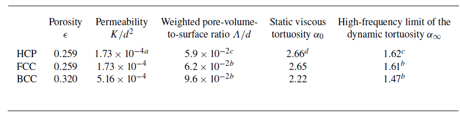
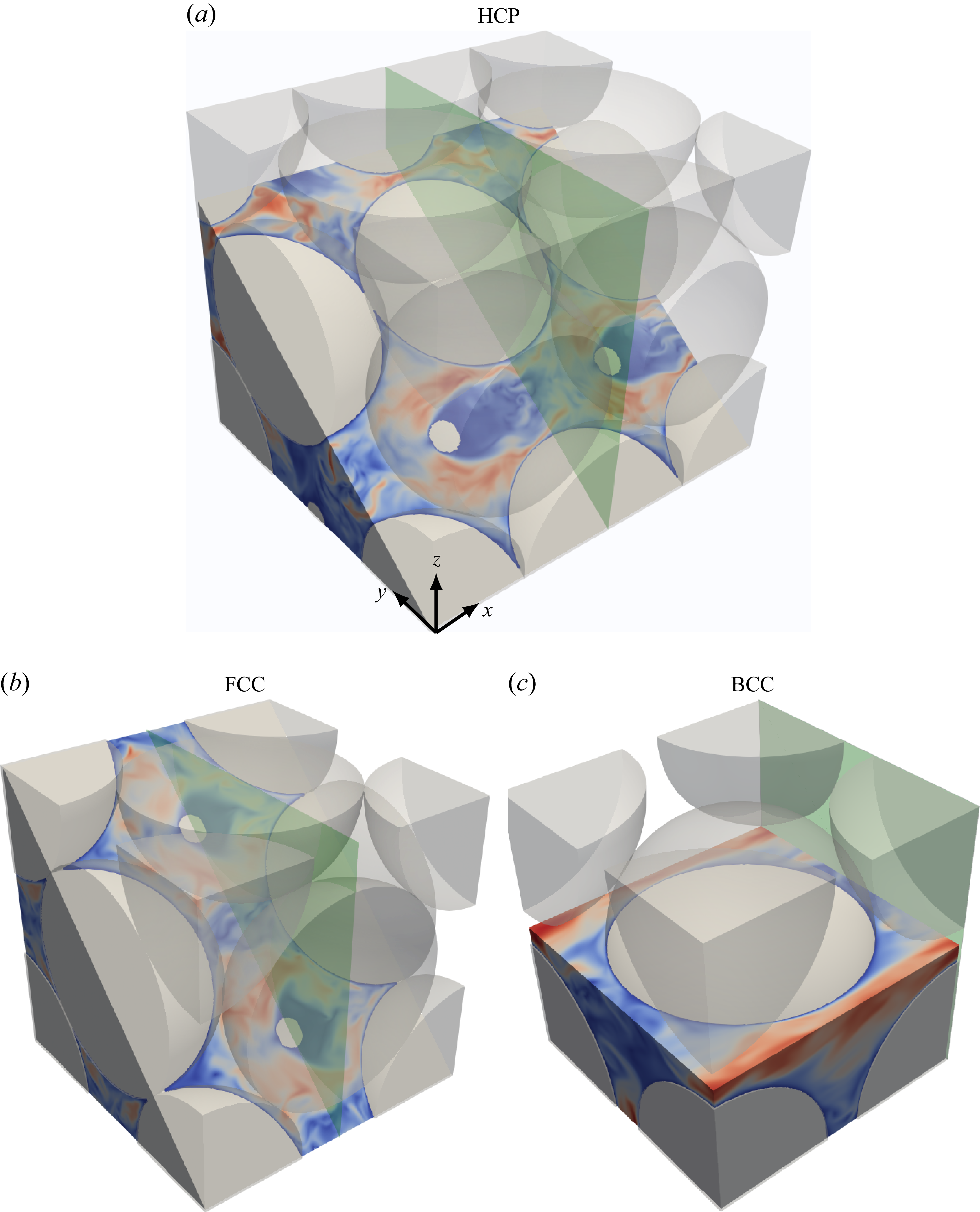
 3y/3+6z/3=0
 y−z=0
 z=d/2
 x=d
 x=2d/2
 x=2d/3
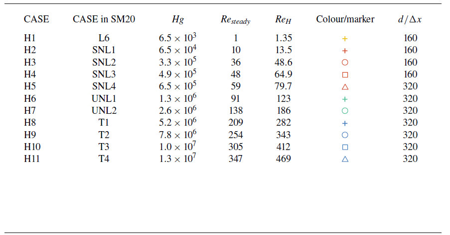
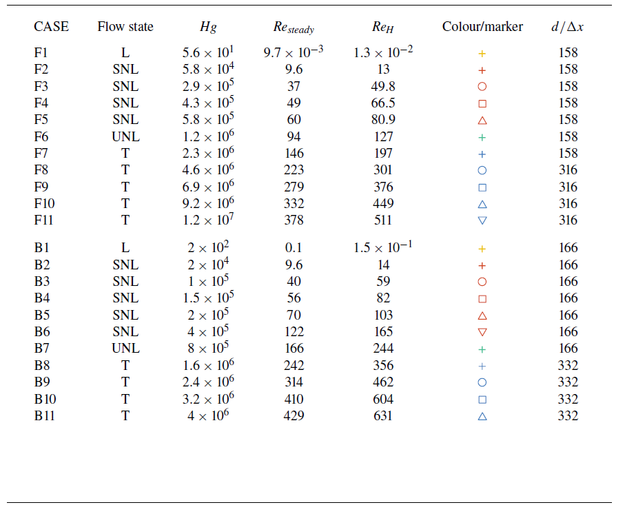
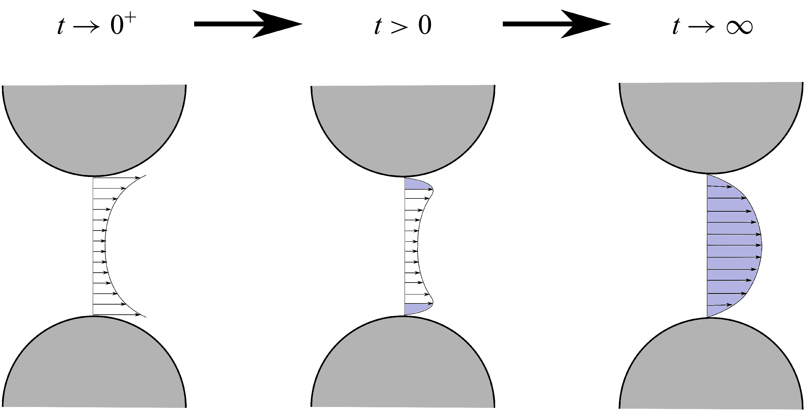
 t→0+
 t>0
 t→∞
 u(x,0)=0
 t→0+
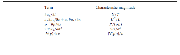
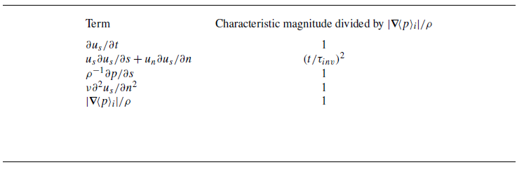
 Hg
 |∇⟨p⟩i|/ρ
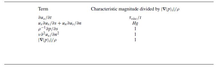
 Hg
 |∇⟨p⟩i|/ρ
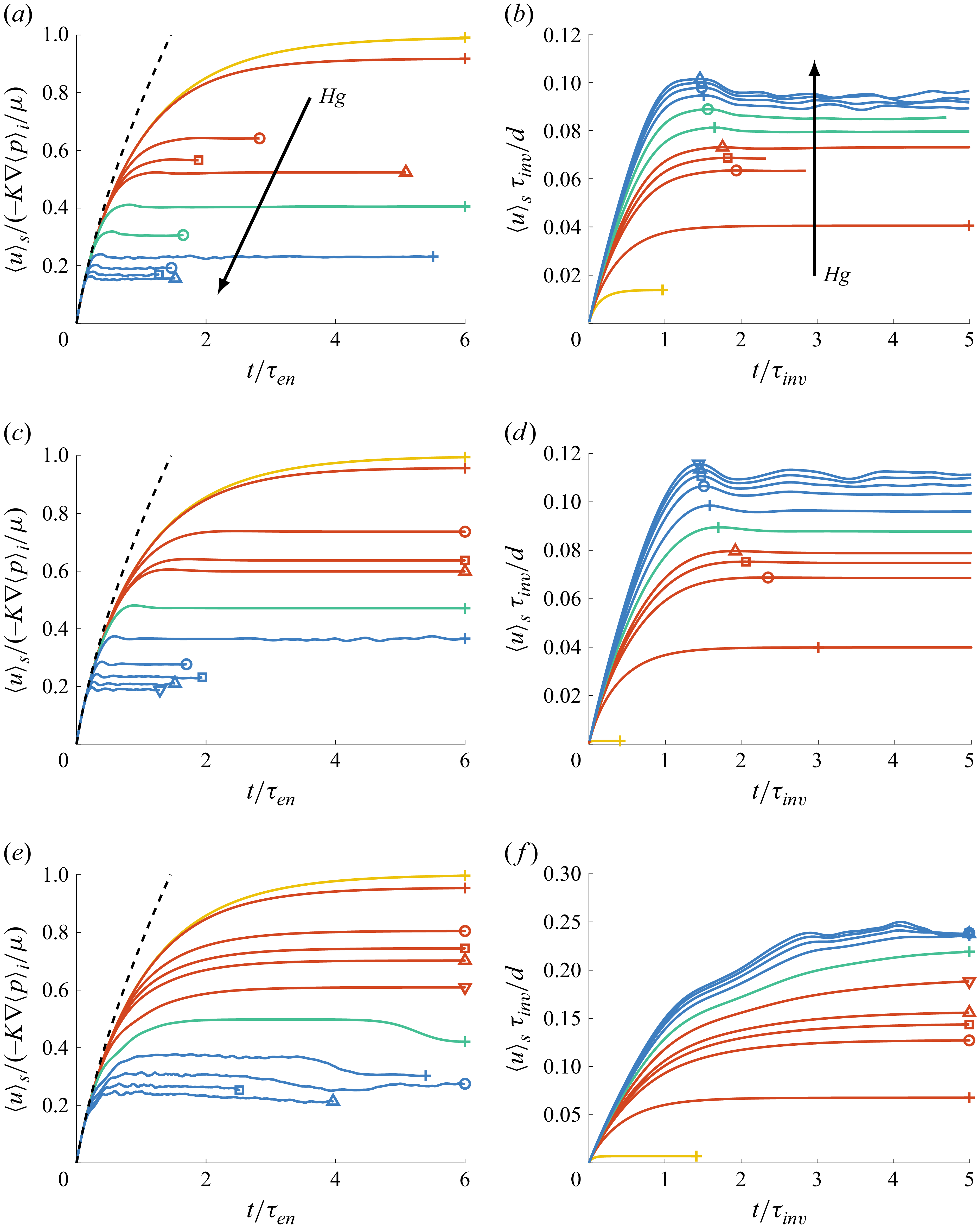
 Hg
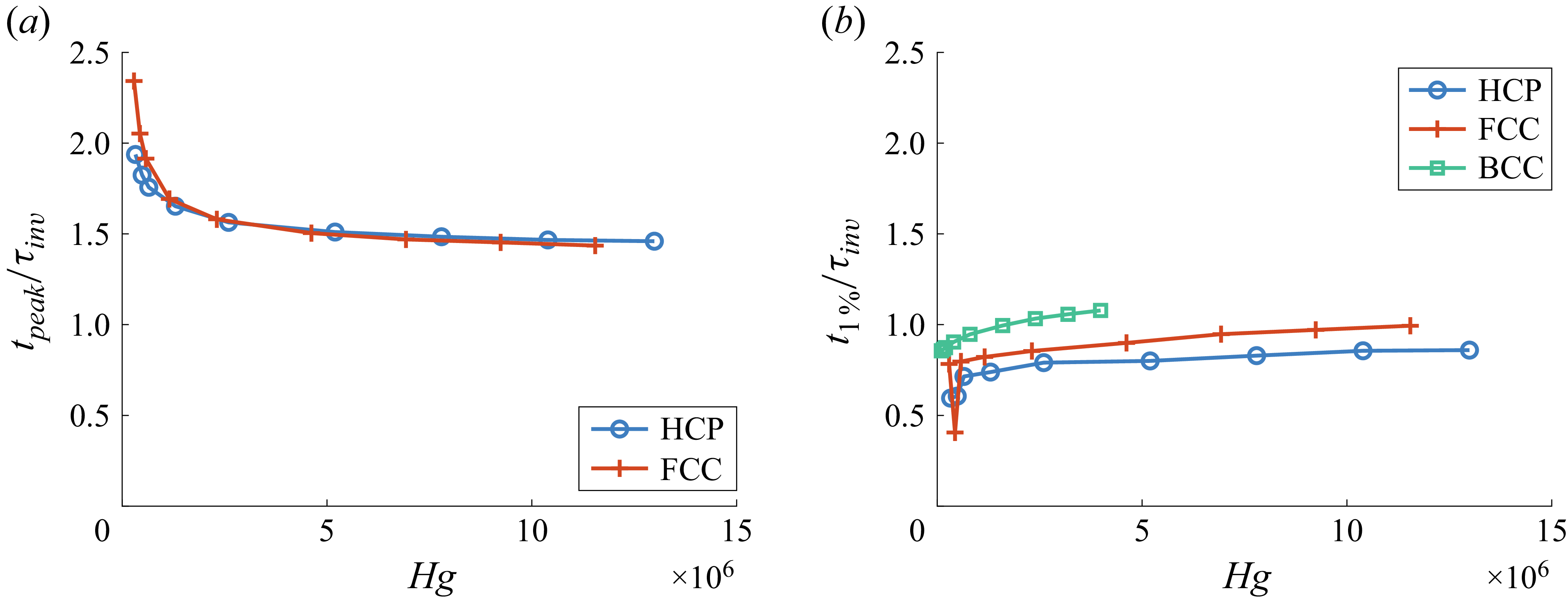
 tpeak
 τinv
 Hg
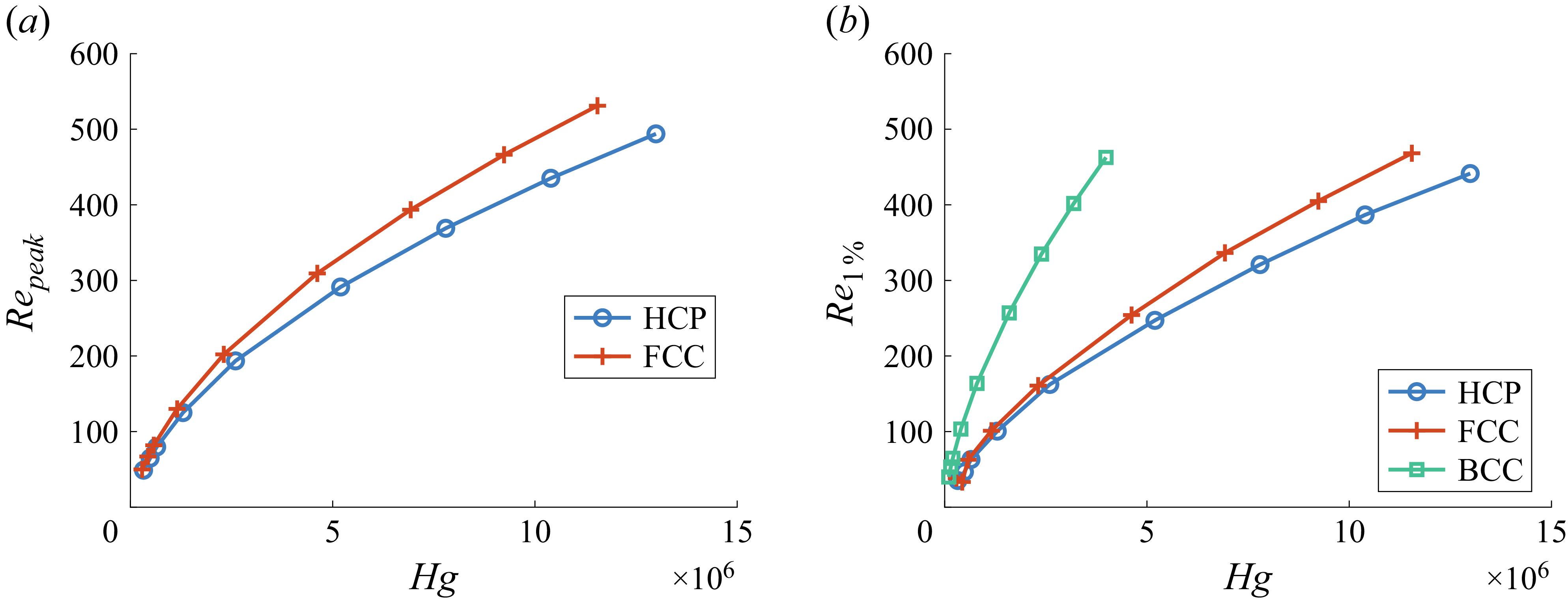
 Repeak
 Hg
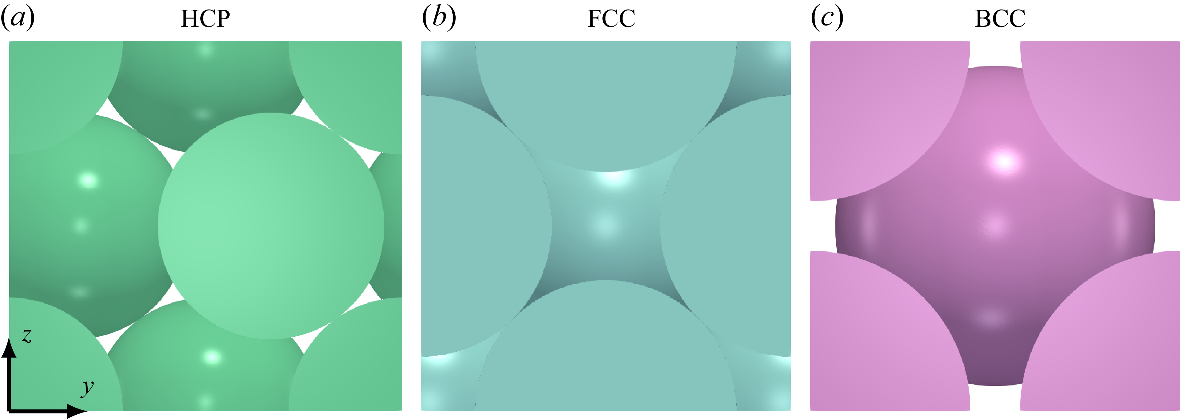
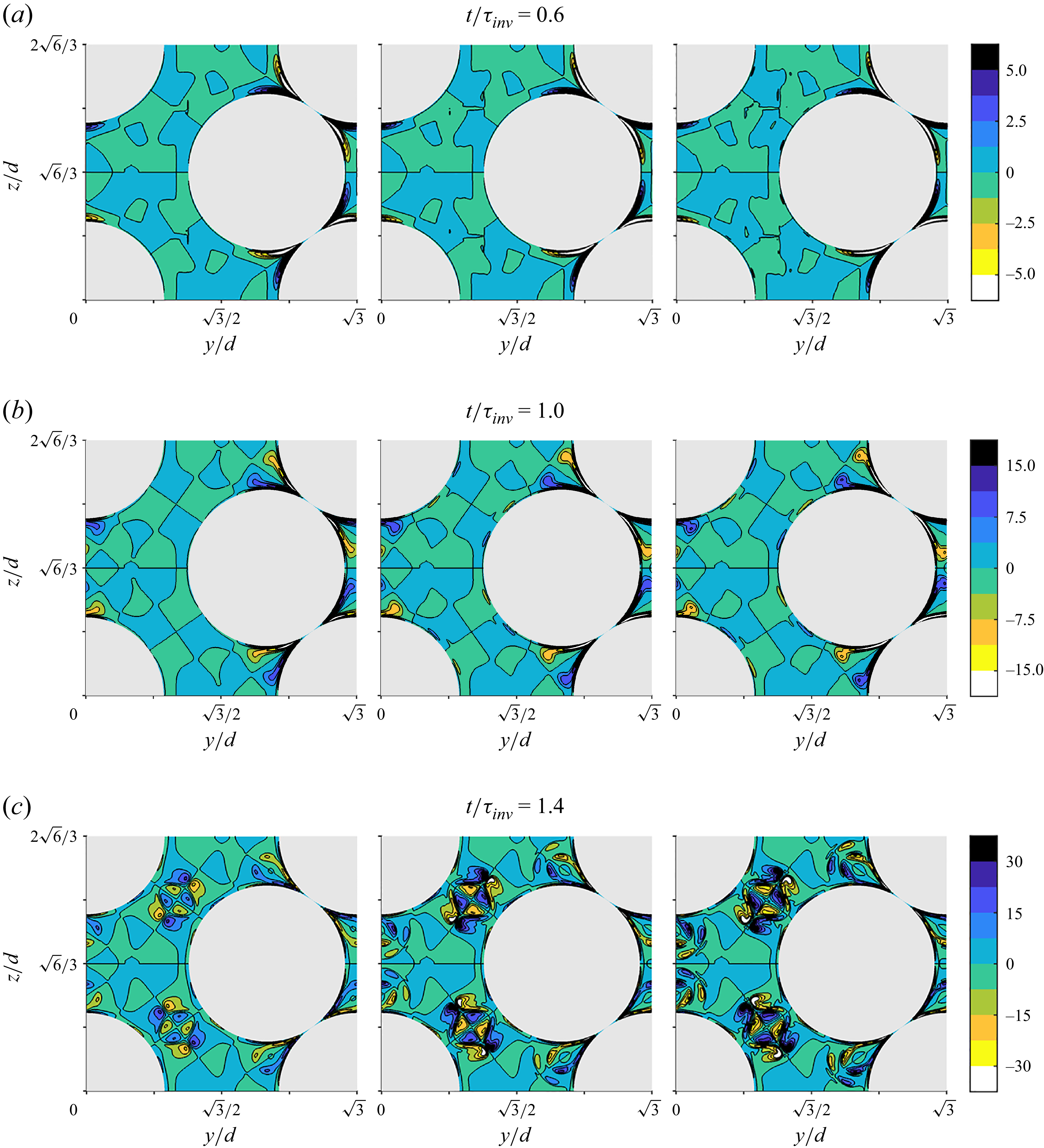
 ωxτinv
 Hg=2.6×10⁶
 Hg=7.8×10⁶
 Hg=1.3×10⁷
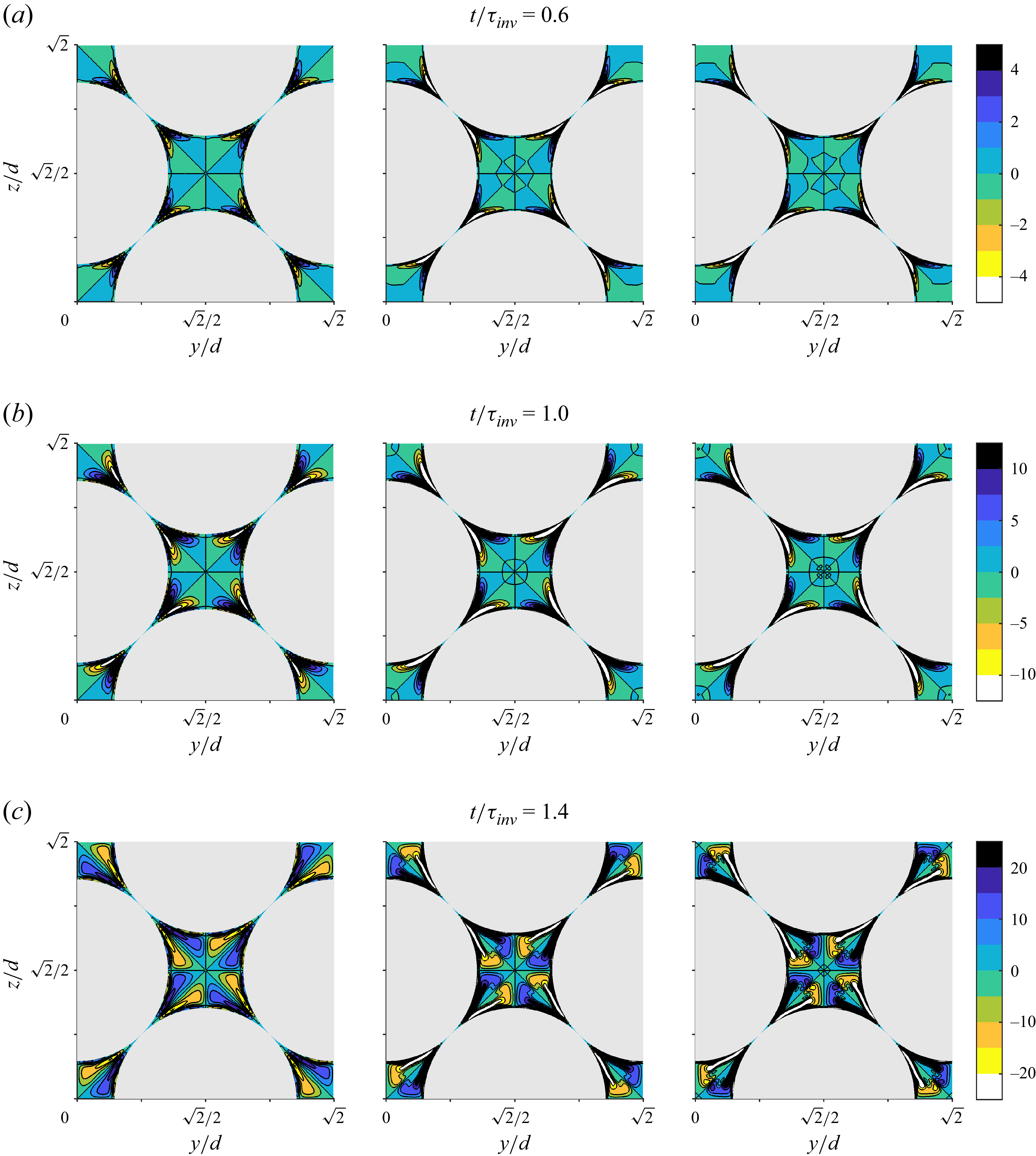
 ωxτinv
 Hg=2.3×10⁶
 Hg=6.9×10⁶
 Hg=1.2×10⁷
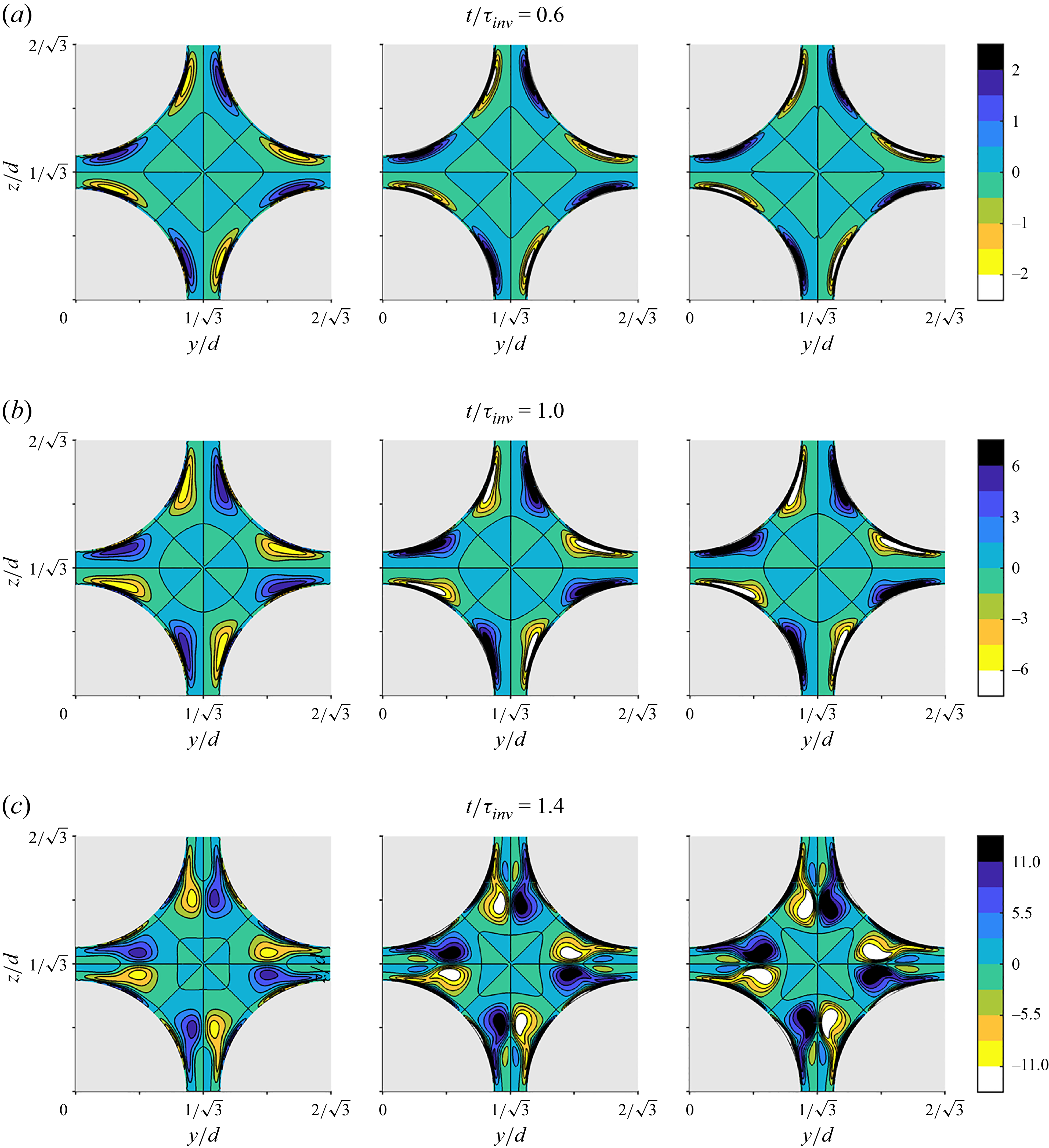
 ωxτinv
 Hg=8×10⁵
 Hg=2.4×10⁶
 Hg=4×10⁶
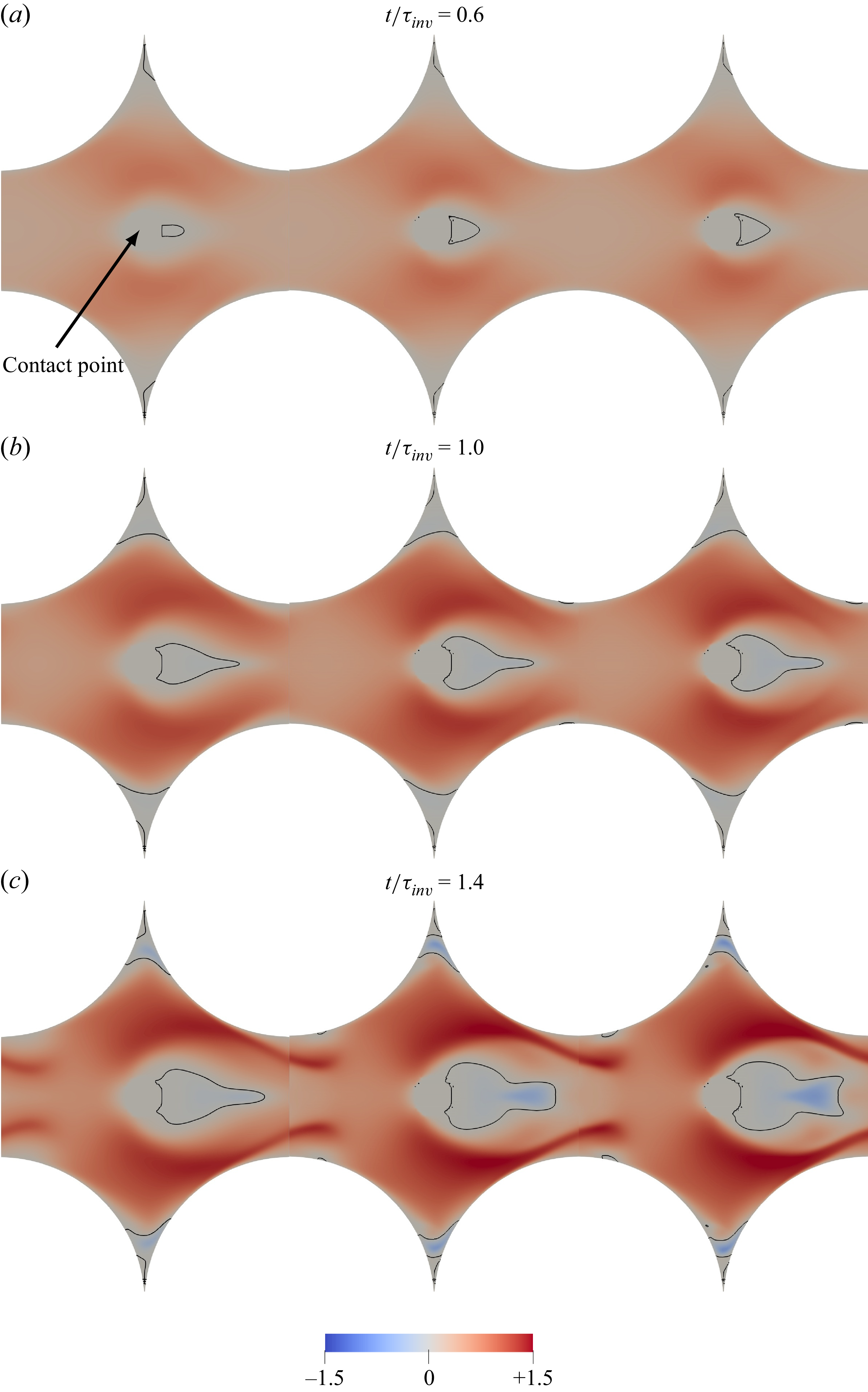
 uτinv/d
 3y/3−6z/3=0
 x
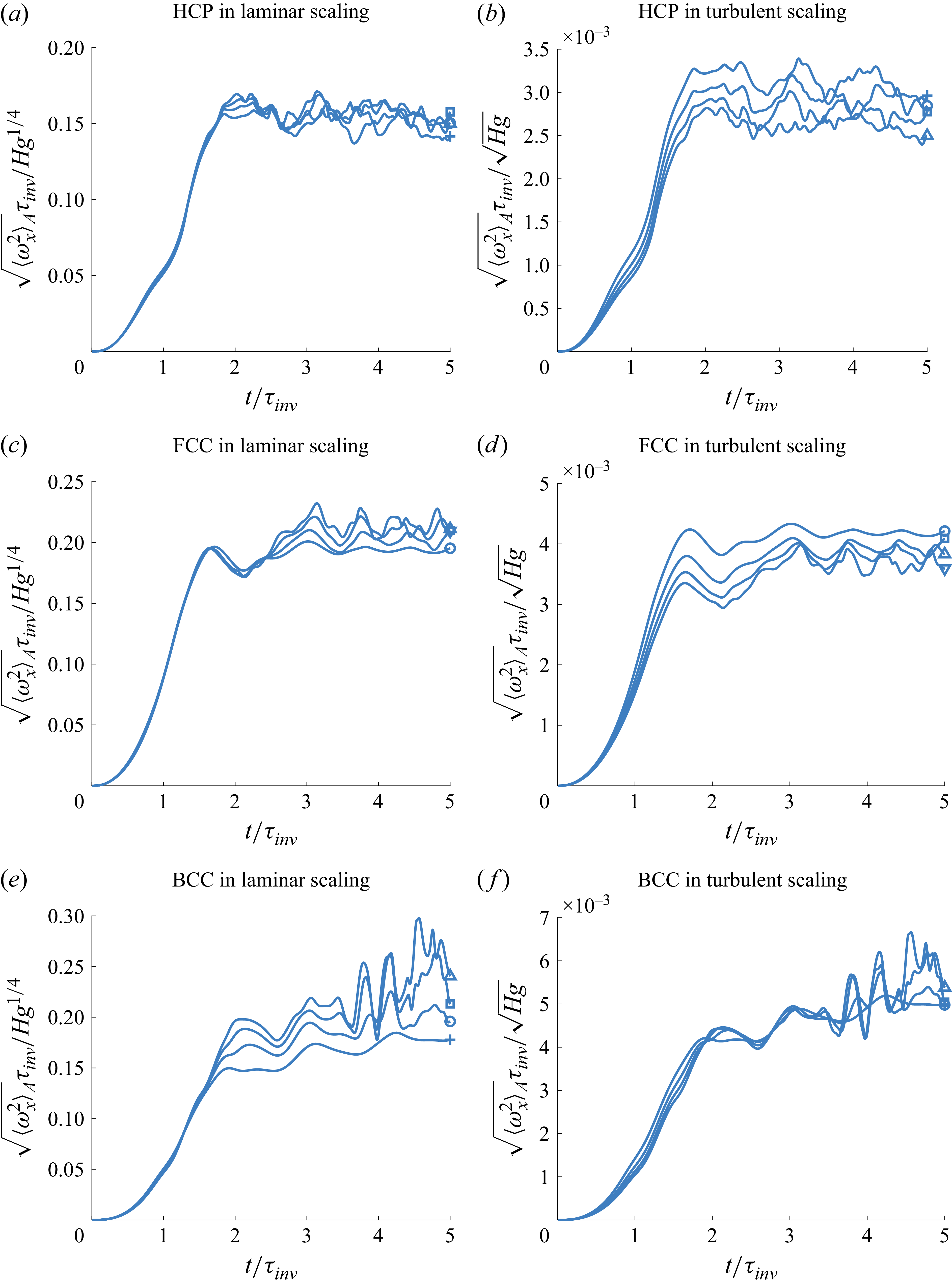
 ⟨ωx2⟩A
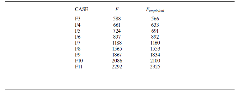
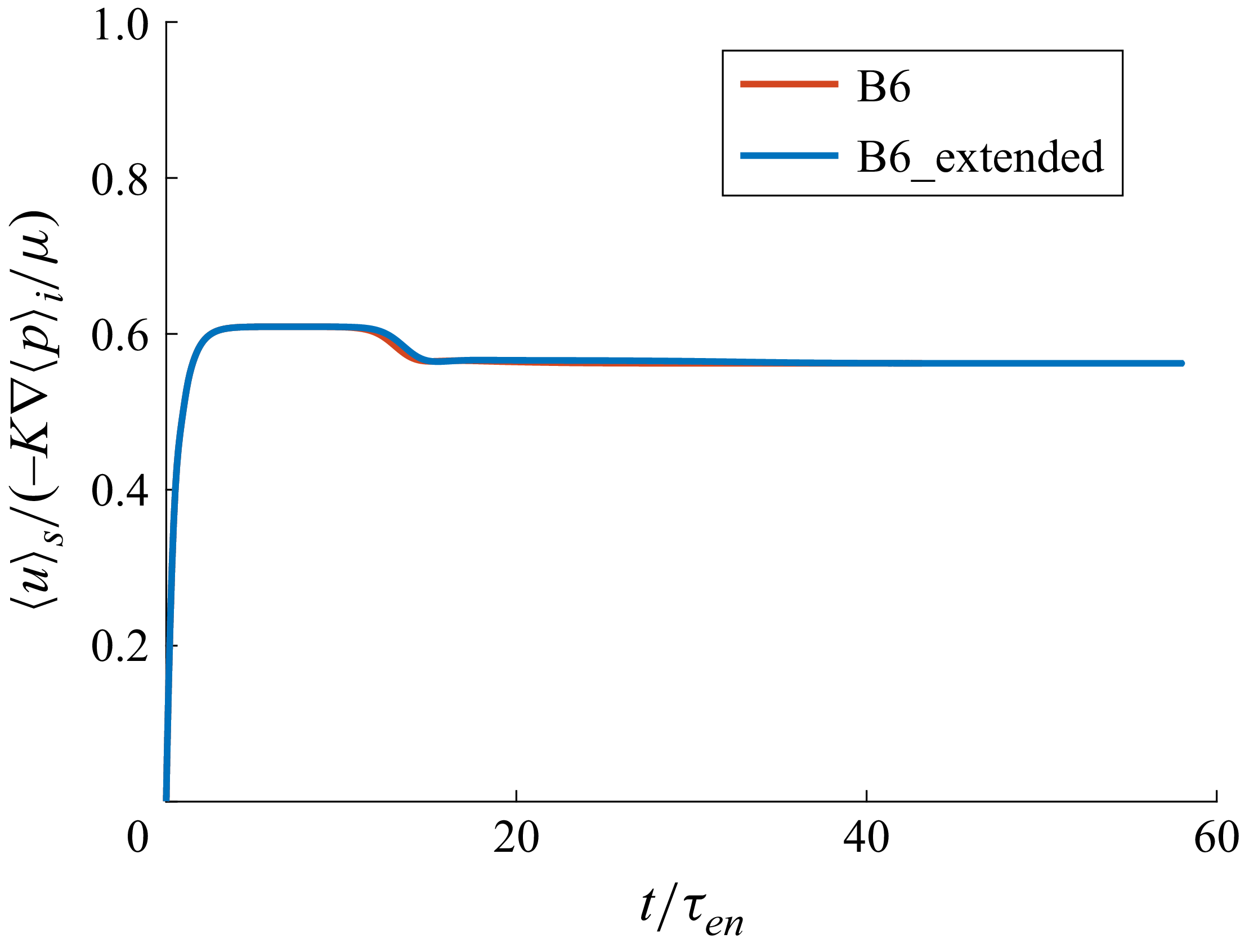
 ⟨u⟩s
 t/τen
 t/τinv=1
 t/τen≈2.26
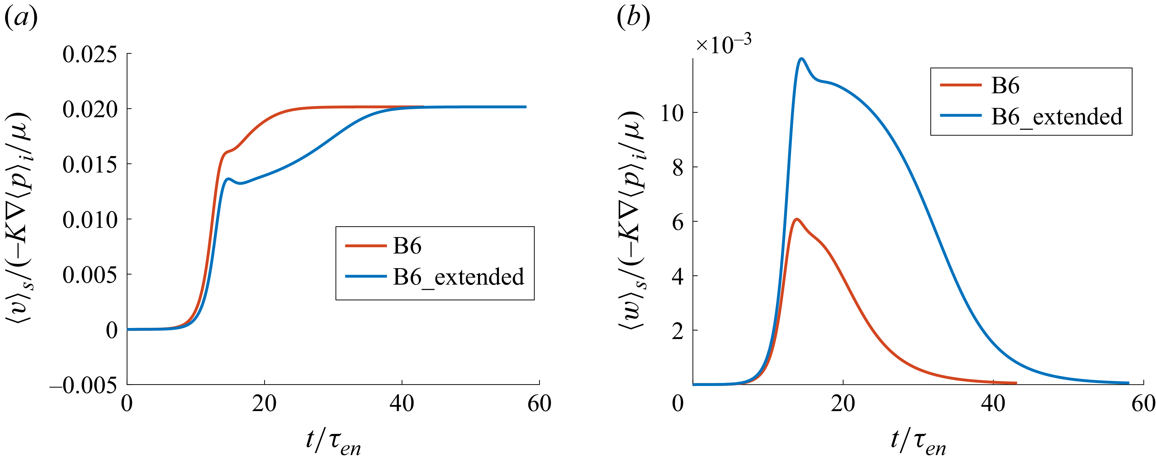
 ⟨v⟩s
 ⟨w⟩s
 t/τen
 t/τinv=1
 t/τen≈2.26


 Open access

