

1. Introduction
The notion that greater economic freedom fuels economic growth has received significant scholarly attention. The cornerstones of economic freedom are secure property rights, freedom to engage in voluntary transactions, access to sound money, freedom to compete and personal choice. The empirical evidence supports the notion that countries with more open markets, secure property rights and limited government under a genuine rule of law tend to achieve consistently higher economic growth in comparison with countries with less economic freedom. Countries with an institutional environment supporting economic freedom tend to achieve higher growth (Azman-Saini et al. Reference Azman-Saini, Baharumshah and Law2010; Bengoa and Sanchez-Robles Reference Bengoa and Sanchez-Robles2003; Berggren Reference Berggren2003; Cole Reference Cole2003; Dawson Reference Dawson1998, Reference Dawson2003; Doucouliagos and Ulubasoglu Reference Doucouliagos and Ulubasoglu2006; Easton and Walker Reference Easton and Walker1997; Gwartney et al. Reference Gwartney, Lawson and Holcombe1999, Reference Gwartney, Holcombe and Lawson2004, Reference Gwartney, Holcombe and Lawson2006; Heckelman Reference Heckelman2000; Scully Reference Scully1988; Vega-Gordillo and Álvarez-Arce Reference Vega-Gordillo and Álvarez-Arce2003), lower unemployment (Grubel Reference Grubel1998), a higher life expectancy (Esposto and Zaleski Reference Esposto and Zaleski1999), lower mortality (Grubel Reference Grubel1998), more equal income distribution (Scully Reference Scully2002), lower poverty rates (Connors and Gwartney Reference Gwartney, Connors and White2010), better quality of health care and education (Stroup Reference Stroup2007), lower pollution (Norton Reference Norton1998), and are more prosperous in the long run (Dawson Reference Dawson2003; de Haan and Siermann Reference De Haan and Siermann1998; Faria and Montesinos Reference Faria and Montesinos2009; Hanke and Walters Reference Hanke and Walters1997; Torstensson Reference Torstensson1994; Ken Farr et al. Reference Ken Farr, Lord and Wolfenbarger1998; Sturm and de Haan Reference Sturm and de Haan2001).
Most of the studies on the nexus between economic freedom and growth are based on cross-country comparisons of different types of institutional frameworks (Helland Reference Helland2016; Klick Reference Klick2010; Spamann Reference Spamann2010). Changes in public policies or legal rules affecting economic freedom can hardly be comparable across countries with heterogeneous sets of economic, legal and political institutions. Since many factors related to economic freedom can vary apart from the legal rules, a cross-country investigation of the effects of economic freedom on economic performance might be subject to several identification frailties. The fundamental problem is statistical identification (Helland and Klick Reference Helland, Klick, Faure and Smits2011), since the omitted variables and institutional heterogeneity in cross-country investigation render policy conclusions questionable. Investigating the effects of economic freedom on economic outcomes under a common institutional environment with greater homogeneity could partially address such bias, and add valuable information to the existing literature (Gwartney and Lawson Reference Gwartney and Lawson2003; Heckelman and Stroup Reference Heckelman and Stroup2005).
We examine the relationship between economic freedom, growth rates and income levels across 407 German districts in the period 1995–2010. We show that there is more institutional homogeneity in the levels of economic freedom within a single country than across countries. Our findings corroborate the notion that even in the homogeneous institutional setup, greater economic freedom is beneficial for prosperity. Our investigation unravels marked disparities in the level of economic freedom across districts. The districts in the southern states (Bavaria and Baden-Württemberg) tend to have a consistently higher level of economic freedom characterized by lower rates of property and business turnover taxation, and a smaller public sector. Contrary to widespread beliefs, our evidence reveals that the former East German districts tend to have higher level of economic freedom than former West German ones. One potential caveat regarding the East's advantage relative to the West is posited by the introduction of a 5.5% unification tax by the Kohl government in 1991 to restore the levels of infrastructure in former East Germany to those enjoyed in the West. We control for the unification tax surcharge in the district-level income tax share of GDP. Even within the West German subsample, the gap in the synthetic index of economic freedom between the northern and southern districts is widespread even though both groups have been paying a common income tax surcharge to finance investment in infrastructure in the former East Germany. Our investigation reveals a persistent north–south economic freedom gap rather than the east–west gap, which traditionally enjoys a widespread scholarly acclaim. Greater economic freedom contributes significantly to income levels and growth rates, although the short-run effects on growth are much less predictable than long-run effects on income levels, yet still statistically significant at conventional levels. Our index of economic freedom across 407 German districts and the counterfactual scenarios indicate that a lower burden of property tax, business turnover tax and income tax, and a lower public debt and public sector employment ratio would substantially promote economic growth and higher income levels within Germany.
Several papers are related to ours. First, Potrafke (Reference Potrafke2013) proposed two indices of economic freedom for German states incorporating the following components: (1) size of government, (2) direct taxation levels and (3) mandatory social insurance and welfare contributions (Fuest et al. Reference Fuest, Bertenrath and Welter2009). He exploits the variation in government ideology as a source of differences in economic freedom. His findings suggest that in the former West German states, right-wing governments under the flagship of Christian Democratic Union (CDU) propagated more economic freedom than the centre-left government of the Social Democratic Party (SDP), whereas no such pattern is found in former East German states. Persistent differences in the level of economic freedom across German Länder warrant further attention to determine whether more economic freedom leads to higher income levels and growth rates. Compared to state-level differences, district-level variations in economic freedom can improve our understanding of the consequences of local institutional variations in growth rates and income levels. Second, Bjornskøv and Foss (Reference Bjørnskov and Foss2008) examine the contribution of economic freedom to entrepreneurship cross-nationally, and show that government size correlates negatively with entrepreneurial activity; sound money tends to boost entrepreneurship while other measures of economic freedom are not significantly correlated with entrepreneurship. It remains an open question whether greater government size dampens economic growth in a subnational setting with a homogeneous institutional environment. Third, Karabegovic et al. (Reference Karabegovic, Samida, Schlegel and McMahon2003) construct a composite measure of economic freedom comprising nine different measures of government size, taxation and labour market regulation for US states and Canadian provinces, proposed by Gwartney et al. (Reference Gwartney, Lawson and Block1996, Reference Gwartney, Holcombe and Lawson2006) and discussed in depth by Carlsson and Lundström (Reference Carlsson and Lundström2002). Their results highlight the beneficial effects of greater economic freedom on both the level and growth of economic activity. And fourth, Bologna et al. (Reference Bologna, Young and Lacombe2016) examine the spatial relationship between institutional quality and economic outcomes across 381 US metropolitan areas using the Stansel (Reference Stansel2013) index of economic freedom for MSAs, allowing for direct and indirect effects of economic freedom on growth and income levels. Their findings suggests that greater economic freedom improves growth and income levels, and that combined direct and indirect effects are quantitatively larger than the direct effects alone, suggesting a strong spillover effect of economic freedom from neighbouring areas.
We tackle and revisit the relationship between economic freedom and growth in a subnational sample of German districts that comprises local rather than state-level or provincial variation in economic freedom. Although greater economic freedom is associated with higher income and growth rates subnationally, the existing evidence in our view is still inconclusive on whether expanding economic freedom tends to improve performance even under a homogeneous institutional environment (Bühn Reference Bühn2011).
The rest of the paper is organized as follows. Section 2 outlines the institutional background of German districts, and presents a new synthetic index of economic freedom for them. Section 3 discusses the empirical strategy. Section 4 presents the results and robustness checks. Section 5 concludes.
2. Institutional background and an index of economic freedom for German districts
In Germany, the Federal Constitution (Grundgesetz für die Bundesrepublik Deutschland) sets out the administrative division divided into (1) states (Länder) and city states (Kreisfreie Städte), (2) government regions (Regierungsbezirke), (3) districts (Kreise), and (4) municipalities (Gemeinden). The districts correspond to NUTS 3-level EU administrative divisions, and are roughly equivalent to counties in the United States. The districts are divided into rural (Landkreise), urban (Stadtkresie) and special-type districts prevalent in the federal states of Saarbrücken, and some parts of Niedersachsen and Nordrhein Westfalen. The latter type of district is a fusion of district-free city states with adjacent rural districts. The district council (Kreistag) is the highest institution of a rural district and is responsible for all fundamental guidelines of regional self-administration. The council is elected every five years, except in Bavaria where it is elected every six years. The highest administrative position is held by an officer who is responsible for the district's administrative functions. In urban districts, a mayor performs a similar function. In some states, rural districts have an additional commission (Kreisausschuss), led by an officer, which takes over certain administrative functions that vary from state to state. The federal and state law delegate an extensive set of fiscal responsibilities to the districts such as (1) taxation of business turnover, (2) collection of income and property taxes and (3) financing of social welfare, health and education programmes.
A synthetic index of economic freedom
We construct a synthetic index of economic freedom by exploiting the variation in levels of taxation, public debt, size of government and public sector employment across German districts. Our index of district-level economic freedom consists of five different components measured as percentage shares of district GDP(1) property taxes, (2) business turnover tax on gross receipts, (3) municipal income, (4) share of municipal value-added tax, (5) share of public debt and additionally (6) share of public employment in total district-level employment. The index is constructed for the period 1995–2010 based on district-level fiscal data. Due to a variety of state-level administrative border reforms, we can construct a cross-sectional index of economic freedom, allowing for the comparison of economic freedom across a full cross-section of districts. One particular caveat should be emphasized. First, we cannot capture the cross-district variation in the levels of regulation in areas such as minimum wage laws and occupational licensing requirements, which are inherent in within-country, and cross-country economic freedom indices. In Germany, minimum wage law and occupational licensing requirements are standardized at the national level, and therefore do not provide sufficient subnational variation to justify their use as district-level policy measures. This is a limitation that per se precludes us from constructing a subnational index of economic freedom comparable with its cross-country counterpart.
The property tax, turnover tax, income tax, VAT and public debt variables are constructed by taking the gross amount of collected tax and debt, and dividing it by the district GDP. The share of public employment is constructed by dividing the number of public sector employees with total employment for each district. The variables are constructed using data from Genesis Regionaldatenbank Deutschland. Let Z = {Z 1i, Z 2i, . . .Zki} denote a vector of components of economic freedom where k = 1, 2, . . .K represents the total number of components and i = 1, 2, . . .N denotes the sample size. For each component, we adjust the potentially excessive variation in the component across districts through a simple unconstrained linear scaling transformation in the following form:
 $$\begin{equation*}
\mathbb{N}( {{Z_k}} ) = \frac{{{Z_{1k}} - \min \{ {{Z_{k1}},{Z_{k2}},...{Z_{kn}}} \}}}{{\max \{ {{Z_{k1}},{Z_{k2}},...{Z_{kn}}} \} - \min \{ {{Z_{k1}},{Z_{k2}},...{Z_{kn}}} \}}},
\end{equation*}$$
where  $\mathbb{N}( {{Z_k}} )$ is a normalized measure of district-level economic freedom ranging from 0 to 1, in which lower values correspond to a lower level of economic freedom, and Z 1k is the original component drawn from the overall component pool {Z k1, Z k2, . . .Zkn}. The linear scaling transformation approach to measuring economic freedom was pioneered by Gwartney et al. (Reference Gwartney, Lawson and Block1996, Reference Gwartney, Holcombe and Lawson2004, Reference Gwartney, Holcombe and Lawson2006) and conveys several advantages such as a direct comparison of district-level differences in similar components of economic freedom. It also mitigates the excessive sampling variations in the distribution of each component that may result in outlier observations. We calculate the level of economic freedom across districts using the principal component analysis. We compute the variance–covariance matrix for the maximum possible combinations of the original components and compute the value of the eigenvectors from the set of weights derived from variance–covariance matrix as follows:
 $$\begin{equation*}
\begin{array}{@{}l@{}} Z_i^{Synthetic} = 0.55{\left( {{\textrm{Property Tax/District GDP}}} \right)_i}\\
\quad +\, 0.32{( {{\textrm{Business Tax/District GDP}}} )_i}\\
\quad +\, 0.56{( {{\textrm{Municipal Income Tax/GDP}}})_i} + 0.08{( {{\textrm{Municipal VAT/GDP}}} )_i}\\
\quad +\, 0.29{( {{\textrm{Public Debt/GDP}}})_i} - 0.42{\left( {{\textrm{Public Sector Employment Share}}} \right)_i}
\end{array}
\end{equation*}$$
This suggests that the synthetic index of economic freedom correlates strongly with the share of property tax in district GDP, the municipal income tax share in GDP, and somewhat strongly with the share of business turnover tax in district GDP, and the share of public debt in district GDP. It correlates weakly with the share of municipal value-added tax in GDP, and it loads negatively on the ratio of public sector employment relative to the total employment. The eigenvalues highlight the areas that appear to be the dominant ones in shaping the level of economic freedom, and indicates which policies can be deployed to affect economic freedom to some degree. The first principal component explains about 75% of the full variation across the indicators, suggesting that cross-district regressions are unlikely to be contaminated by the unobserved latent variation in economic freedom. Eigenvectors with eigenvalues below unity are excluded from the scored principal components to ensure that the most powerful eigenvector is selected reflecting the maximum variation in economic freedom. The highest eigenvector has an absolute value slightly above 1.95 and a Cronbach (Reference Cronbach1951) coefficient in the acceptable range (α = 0.54), indicating an internally consistent measure of economic freedom.
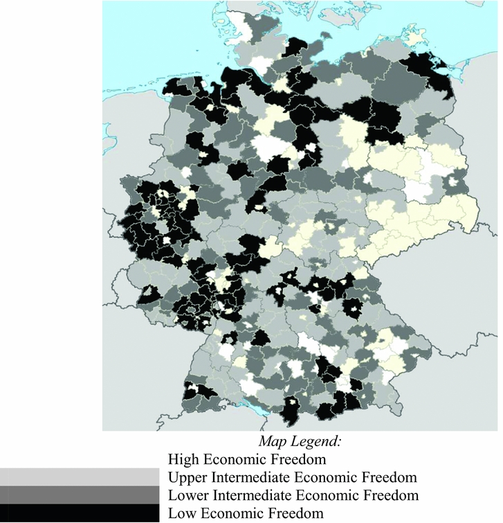
In Figure 1, a spatial distribution of the synthetic index of economic freedom is presented. The evidence suggests that the distribution of economic freedom within Germany is uneven. Low levels of economic freedom are clustered in northwest and West German states. In the West German subsample, districts in Bavaria and Baden-Württemberg tend to have higher levels of economic freedom than other West German districts. Districts in West German states have significantly lower levels of economic freedom than their eastern counterparts (p-value = 0.000).Footnote 1 Southern districts do not seem to have more economic freedom than former eastern districts (p-value = 0.365). A simple comparison of economic freedom differences across different geographical areas of Germany highlights markedly lower levels of economic freedom in north German districts compared to the rest of the country (p-value = 0.094).
Synthetic index of economic freedom across German districts.

Comparing the synthetic index across districts advocates two important patterns. First, the east–west gap has not only disappeared but has been reversed in favour of the former eastern districts. Second, the east–west gap has been replaced by the north/west–south/east gap. The east/south cluster tends to have substantially higher levels of economic freedom than the north/west cluster (p-value = 0.000), which suggests that the gap between the two gradients does not seem to be an artefact.
3. Empirical strategy
The goal of our empirical strategy is to examine consistently the contribution of economic freedom to the district growth rates and income levels. Our empirical strategy sets to distinguish between the short-run effect of economic freedom (on growth rates) and its long-run effect (on income levels). For a full cross-section of districts, we estimate the following set of the core model specification:
 $$\begin{eqnarray}
\ln {y_{i,j,k,l}} &=& \ln A + {{\hat{\gamma }}_1} \cdot E{F_{i,j,k,l}} + {{\hat{\alpha }}_1}\ln {y_{0,i,j,k,l}} + {{\bf X^{\prime}}}\beta \nonumber\\
&& +\, \sum\limits_{j = 1}^J {{\hat{\phi }}_j} \cdot 1\left[ {i \in j} \right] + \sum\limits_{k = 1}^K {{{\hat{\alpha }}_k} \cdot 1[ {i \in j \in k}]}\nonumber\\
&& + \sum\limits_{l = 1}^L {{{\hat{\Theta }}_l} \cdot 1[ {i \in j \in k \in l}]} + {\varepsilon _{i,j,k,l}}
\end{eqnarray}$$
 $$\begin{eqnarray}
\Delta \ln {y_{i,j,k,l}} &=& \ln A + {{\hat{\lambda }}_1} \cdot E{F_{i,j,k,l}} + {{\hat{\omega }}_1} \cdot \ln {y_{0,i,j,k,l}} + {{\hat{\omega }}_2} \cdot \ln {y_{i,j,k,l}} +\, {{\bf X^{\prime}}}\alpha\nonumber\\
&& +\, \sum\limits_{j = 1}^J {{\mu _j} \cdot 1\left[ {i \in j} \right] + \sum\limits_{k = 1}^K {{\theta _k} \cdot 1\left[ {i \in j \in k} \right]} }\nonumber\\
&& +\, \sum\limits_{l = 1}^L {{\Gamma _l} \cdot 1\left[ {i \in j \in k \in l} \right]} + {u_{i,j,k,l}}
\end{eqnarray}$$
where y is the per capita income level and ∆ln y is the average growth rate of for i-th district indexed by i = 1, 2, . . .N, and X is the vector of structural control variables and comprises the sectoral value-added shares, investment/GDP ratio and the fraction of the district's population with tertiary education. The key covariate of interest is EF, which denotes the synthetic index of economic freedom. The coefficients of interest are  ${\hat{\lambda }_1}$, which captures the short-run effect of economic freedom, and
 ${\hat{\gamma }_1}$, which captures the long-run effect of economic freedom. Following Barro (Reference Barro1991), an initial level of per capita income, denoted by y 0, is added to the growth covariates. It allows us to control whether or not the effect of economic freedom on growth and income is the result of the convergence to the mean. Short-run and long-run empirical specifications of the cross-district growth model contain the set of unobserved effects confounding the relationship between economic freedom, growth and income levels. The set of spatial fixed effects is introduced at the administrative regional level, indexed by j = 1, 2. . .J, government regional level, indexed by k = 1, 2. . .K, and at the state level, indexed by l = 1, 2, . . .L. The covariates denoted by 1[ · ] are the indicator functions for the set of administrative regions, government regions and the federal state. The terms ε and u capture the stochastic disturbances.
A valid inference on  ${\hat{\gamma }_1}$ and
 ${\hat{\lambda }_1}$ can be undermined if the stochastic disturbances are correlated across districts, which renders the estimated parameters inconsistent in spite of controlling for the unobserved effects. The failure to control for a within-cluster residual correlation is likely to yield underestimated standard errors, over-rejecting the null, and triggering Moulton bias (Moulton Reference Moulton1986, Reference Moulton1990) despite the inclusion of multiple fixed effects (Bertrand et al. Reference Bertrand, Duflo and Mullainathan2004; Davis Reference Davis2002; Kezdi Reference Kezdi2004; Pepper Reference Pepper2002). We overcome the multiway serially correlated disturbances using a non-nested multiway clustering scheme (Cameron et al. Reference Cameron, Gelbach and Miller2011) simultaneously at district, administrative regional, government regional and state levels by deploying a multiway error component model under an i.i.d. residual distribution assumption. Compared to the one-way clustering schemes such as the robust variance–covariance OLS matrix estimator (Huber Reference Huber1967; White Reference White1980), the non-nested multiway clustering estimator facilitates a valid inference on the key parameters even in the presence of a non-zero within-cluster residual correlation (Arellano Reference Arellano1987; Liang and Zeger Reference Liang and Zeger1986; Hansen Reference Hansen2007; Pfefferman and Nathan Reference Pfeffermann and Nathan1981; Wooldridge Reference Wooldridge2003).
We address the potential discrepancy between the average effect and the full distributional effect of economic freedom on income and growth disparities by composing a conditional function of the outcome variables across different tails of the distribution. Let q∈{0,1} denote a quantile of the empirical distribution function splitting the data into proportions q below and 1−q above the conditional quantile function. We construct the quantile-specific estimate of economic freedom on two district-level outcomes by estimating the set of objective non-differential functions:
 $$\begin{equation}
Q\left( {{\gamma _1}} \right) = \sum\limits_{i:\ln y \ge {{\bf X}}_i^{{\bf {\prime}}}\beta }^N {q\left| {\ln {y_i} - {{\bf X}}_i^{{\bf {\prime}}}{\beta _q}} \right|} + \sum\limits_{i:\ln y < {{\bf X}}_i^{{\bf {\prime}}}\beta }^N {\left( {1 - q} \right)} \left| {\ln {y_i} - {{\bf X}}_i^{{\bf {\prime}}}{\beta _q}} \right|
\end{equation}$$
 $$\begin{equation}
Q\left( {{\lambda _1}} \right) = \sum\limits_{i:\Delta \ln y \ge {{\bf X}}_i^{{\bf {\prime}}}\beta }^N {q\left| {\Delta \ln {y_i} - {{\bf X}}_i^{{\bf {\prime}}}{\beta _q}} \right|} + \sum\limits_{i:\Delta \ln y < {{\bf X}}_i^{{\bf {\prime}}}\beta }^N {\left( {1 - q} \right)} \left| {\Delta \ln {y_i} - {{\bf X}}_i^{{\bf {\prime}}}{\beta _q}} \right|
\end{equation}$$
where Q(γ1) and Q(λ1) denote the quantile-specific effect of economic freedom on growth and income levels per Q( · ) quantile while X′iβq represents the full set of covariates. We mitigate the heteroscedasticity of residual distribution and serially correlated stochastic disturbances and estimate the heterogeneous effect of economic freedom on growth using the robust variance–covariance matrix by Parente and Santos Silva (Reference Parente and Santos Silva2016), adjusting the standard errors for serially correlated stochastic disturbances at various layers of administrative division. Let g = 1, 2. . .G denote the number of clusters each with ng = n elements. We allow λ1 and γ1 to differ across tail proportions in the presence of a non-zero intra-cluster residual correlation:
 $$\begin{eqnarray}
\tilde{\gamma }_1^q &=& \arg \mathop {\min }\limits_q \frac{1}{G}\sum\limits_{g = 1}^G\nonumber\\
&&\times\left\{ \sum\limits_{\ln {y_i} > X_{ig}^{\prime}{\beta _q}} q\left| {\ln {y_{gi}} - X_{ig}^{\prime}{\beta _q}} \right| +\, \sum\limits_{ln{y_i} < X_{ig}^{\prime}{\beta _q}} {\left( {1 - q} \right)\left| {\ln {y_{gi}} - X_{ig}^{\prime}{\beta _q}} \right|} \right\}
\end{eqnarray}$$
 $$\begin{eqnarray}
\tilde{\lambda }_1^q &=& \arg \mathop {\min }\limits_q \frac{1}{G}\sum\limits_{g = 1}^G \nonumber\\
&&\times\left\{ \sum\limits_{\Delta \ln {y_i} > X_{ig}^{\prime}{\beta _q}} q\left| {\Delta \ln {y_{gi}} - X_{ig}^{\prime}{\beta _q}} \right| + \sum\limits_{\Delta ln{y_i} < X_{ig}^{\prime}{\beta _q}} {\left( {1 - q} \right)\left| {\Delta \ln {y_{gi}} - X_{ig}^{\prime}{\beta _q}} \right|} \right\} \nonumber
\\
\end{eqnarray}$$
where  $\tilde{\lambda }_1^q$ and
 $\tilde{\gamma }_1^q$ denote the full distributional effect of economic freedom on growth and income levels. When the residuals are i.i.d. and in the absence of a non-zero intra-cluster correlation the underlying estimators are equivalent to the heteroscedasticity-robust estimator (Chamberlain Reference Chamberlain and Sims1994; Kim and White Reference Kim, White, Fomby, Hill, Jeliazkov, Esanciano and Hillebrand2003; Koenker and Bassett Reference Koenker and Bassett1978; Powell Reference Powell1986). Facilitating asymptotically valid standard errors under heteroscedasticity and model misspecification, we allow for the presence of heteroscedasticity and intra-class residual correlation following Machado and Santos Silva (Reference Machado and Santos Silva2000).
4. Data
Outcomes
Our outcome variables are income level and the growth rate of per capita income. The income level is constructed as the per capita GDP is denoted in euros and expressed in 2011 constant prices. In the full cross-section of districts, we use the income level in the year 2011 as the final observation year. The growth rate of per capita GDP is constructed as a simple unweighted average rate of change in per capita income (at constant 2011 prices) in the period 1995–2011. Both outcomes are constructed using data from GENESIS Regionaldatenbank.
Covariates
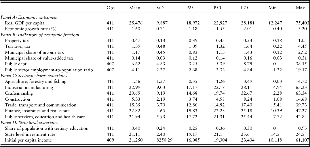
The set of control variables consists of the sectoral GDP shares broken down into the share of agriculture, the share of industrial manufacturing, craftsmanship, construction, and the share of trade, financial services and public services in the total district output. Data on the investment/GDP ratio are not available at the district level. To remedy this, we compute the state-level investment/GDP ratio as a proxy for the district-level investment rate from Volkswirtschaftliche Gesamtrechnungen von Länder. As a proxy for human capital investment we compute, using data from GENESIS Regionaldatenbank, the share of the district's resident population that successfully completed university exams. Both measures allow us to address the omitted variable bias inherent in any growth regression setup arising from the neglect of common growth determinants (Mankiw et al. Reference Mankiw, Romer and Weil1992). In Table 1, key descriptive statistics on income level, growth rates and full covariate set are presented in detail.
Descriptive statistics

5. Results
Baseline OLS results
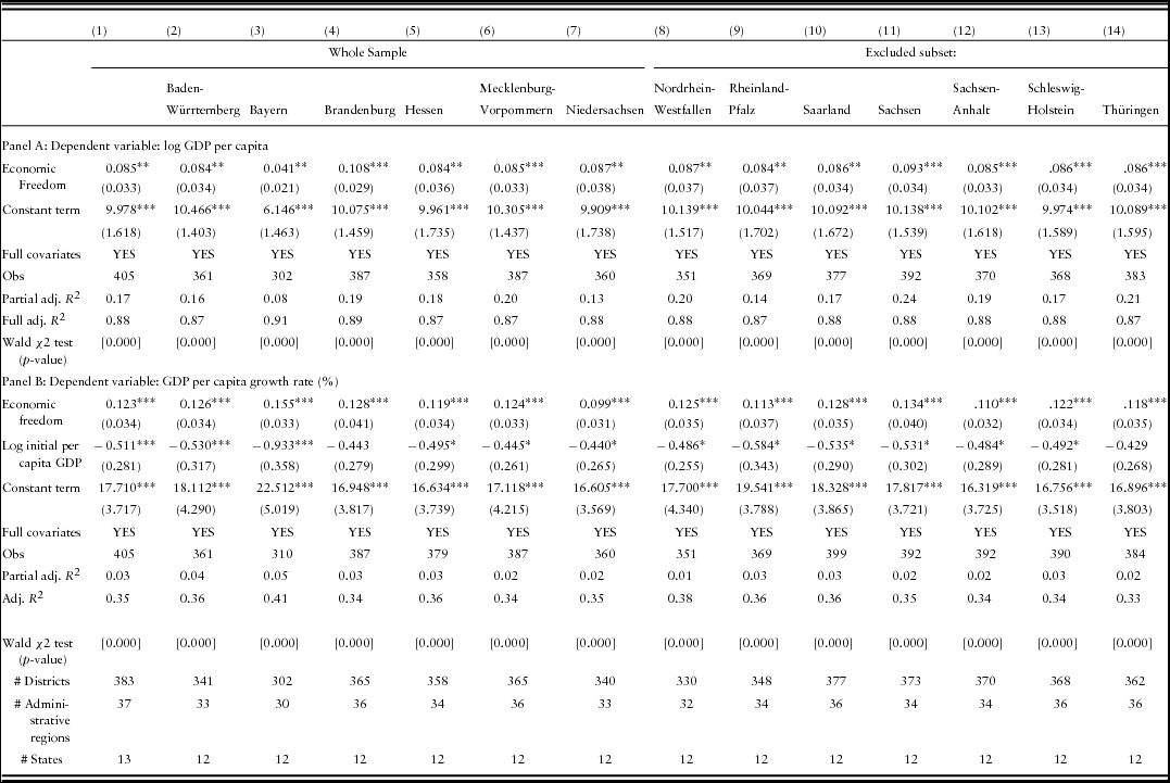
In Table 2, we present the effects of economic freedom on income levels and growth rates for the full sample of districts. In Panel A, the effects of economic freedom on income levels are presented while Panel B presents short-run effects of economic freedom on cross-district growth rates. In column (1), the full sample estimate indicates that a 1 basis point increase in synthetic index of economic freedom is associated with an 8.5% increase in income level. The point estimate is economically large and statistically significant at 5%. The size of the long-run effect of economic freedom indicates a strong and persistent relationship with respect to income levels. In particular, a 1 basis point differences in the synthetic index of economic freedom roughly corresponds to the observed quantitative difference between the Neunkirchen (Saarland) and Günzburg (Bayern) districts, which is approximately equivalent to the distance between the median and 80th percentile of the distribution. Our evidence readily suggests that the synthetic district-level index of economic freedom alone explains up to 17% of the per capita income variance across districts, while the full covariates explain up to 88% of cross-district income differences.
Economic freedom, growth and income levels across German districts

Notes: Table 2 presents the effects of economic freedom on real GDP per capita and its growth rate. The dependent variables are the log per capita GDP and the GDP growth rate. Each regression specification contains the set of unobserved state-fixed effects and administrative-fixed effects. The set of control variables in each underlying specification consists of the log initial per capita GDP, log state-level investment/GDP ratio and the fraction of population with successfully completed university entrance exams. The standard errors are adjusted for arbitrary and non-random disturbances arising from heteroscedastic distribution of error variance and serially correlated residuals simultaneously at district level, administrative cluster level and state level using Cameron et al. (Reference Cameron, Gelbach and Miller2011) multiway clustering scheme and the appropriate moment-based empirical distribution function. Asterisks denote statsitically significant regression coefficients at 10% (*), 5% (**), and 1%(***), respectively.
The long-run effect of economic freedom on income level is stable across multiple subsamples. In columns (2) and (3), the districts from Bayern and Baden-Württemberg are split off from the full sample. In spite of the coefficient drop to 0.084 and 0.041 as a result of excluding high-freedom districts, the evidence confirms the beneficial effect of economic freedom on income level, since the magnitudes are significant at 5%. In columns (4) through (6), the effect of economic freedom on income level jumps back to its full sample counterpart once districts from the states of Brandenburg, Hessen and Mecklenburg-Vorpommern are excluded from the full sample. In Panel B, we reject the notion that the beneficial effect of economic freedom is the result of the convergence to the mean. In the full set of specifications, the beneficial effect of economic freedom is conditional on the initial per capita income. The coefficient on initial per capita income is both negative and statistically significant at 5%. Greater economic freedom tends to foster growth after taking into account that districts with lower initial per capita income have grown faster than the districts with high initial per capita income. Excluding the districts with below-average per capita income, the coefficient on initial per capita income is substantially weaker, which is expected since these districts comprise the high-growth cluster in the post-unification period.
The fraction of the cross-district variation in income levels explained by economic freedom alone is stable in the range between 13 and 20%. Our evidence suggests that the main source of disparity in the magnitude of the effect arises from the composition of the sample. Excluding former West German states from the full samples tends to underscore the full-sample effect of economic freedom on growth, while excluding former East German districts tends to raise the magnitude of the effect considerably. This is further indicated in columns (11), (12) and (14), where the districts from three former East German states are excluded from the core sample.
In Panel B, the short-run effects of economic freedom on growth are presented. In column (1), a 1 percentage point increase in the synthetic index of economic freedom is associated with a 12.3% improvement in the rate of economic growth, holding everything else constant, and conditional on initial per capita income. The coefficient on initial per capita income (-0.511 with cluster-robust SE = 0.034), highlights a rapid degree of convergence between former East and West German districts from 1995 onwards. The effect appears to be stable across subsamples. Excluding districts from the high-freedom states such as Bayern and Baden-Württemberg tends to raise the underlying magnitude of the effect considerably to 0.155 (cluster-robust SE = 0.033), and 0.126 (cluster-robust SE = 0.034) compared to column (1). The beneficial effect of economic freedom on growth does not disappear across columns (9) to (14), where similar exclusion checks are performed on the remaining states. Our evidence indicates large growth gains from greater economic freedom. Taking our preferred specification in column (1), expanding the level of economic freedom from the 25th percentile (Steinfurt, Nordrhein-Westfalen) to the 75th percentile (Cham, Bayern) is associated with a 19% increase in growth rate suggesting that the growth dividend from greater economic freedom is considerable.
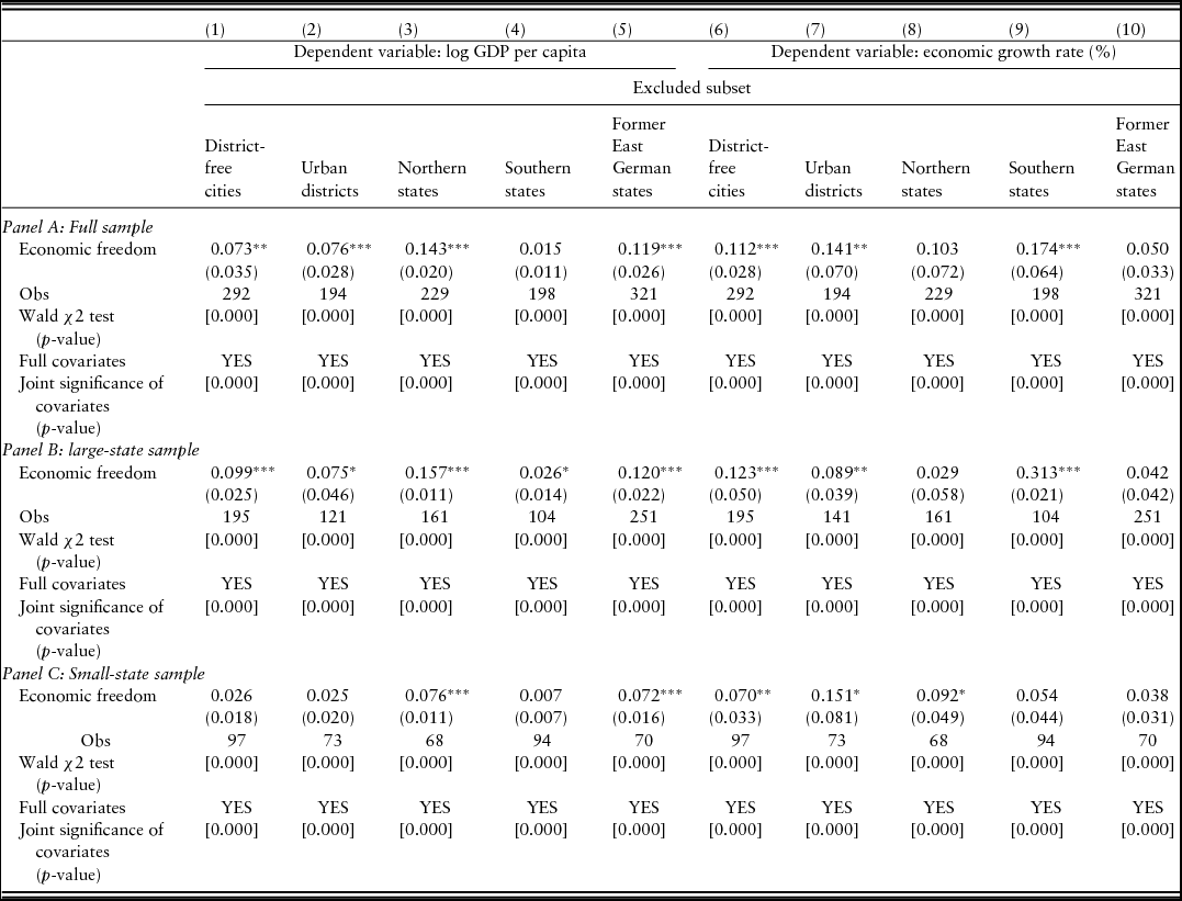
In Table 3, we examine the robustness of the key economic freedom parameters across subsamples. The robustness of the key parameters is assessed by splitting district types off the full sample specification. The effect of economic freedom on growth rate and income level is replicated on the core sample, large- and small-state samples to unravel the sensitivity of economic freedom in influencing per capita incomes and growth. In Panel A, the evidence confirms the positive effect of freedom on income level, which does not appear to be driven either by the institutional type of district or by the geographic composition of the sample. In Panel B, the effect of freedom on income appears to be stable in large-state subsamples while the growth effect of economic freedom appears to be slightly weaker. Lastly, in Panel C, the beneficial effects of economic freedom on per capita incomes are confirmed on a small-state sample whereas the short-run effects of freedom on growth rate tend to be slightly weaker and marginally significant at borderline levels. The effects of economic freedom are not driven by the institutional type of districts either. The underlying coefficient on economic freedom is in the 0.073 to 0.143 coefficient range across (long-run) income level regression specifications, and in the 0.103 to 0.174 coefficient range for cross-district growth regressions. The effects of economic freedom on both economic outcomes tend to be particularly stronger in larger states and slightly weaker in smaller states.
Effects of economic freedom on income level and growth of German districts across various subsamples

Notes: Table 3 presents the effects of economic freedom on income level and its growth rate over time across various sub-samples. The standard errors are robust against heteroscedasticity and serially correlated stochastic disturbances using the non-nested empirical distribution function based on the moment conditions and Cameron et al. (Reference Cameron, Gelbach and Miller2011) multiway clustering scheme. Asterisks denote statistically significant regression coefficients at 10% (*), 5% (**) and 1% (***), respectively.
Effect heterogeneity
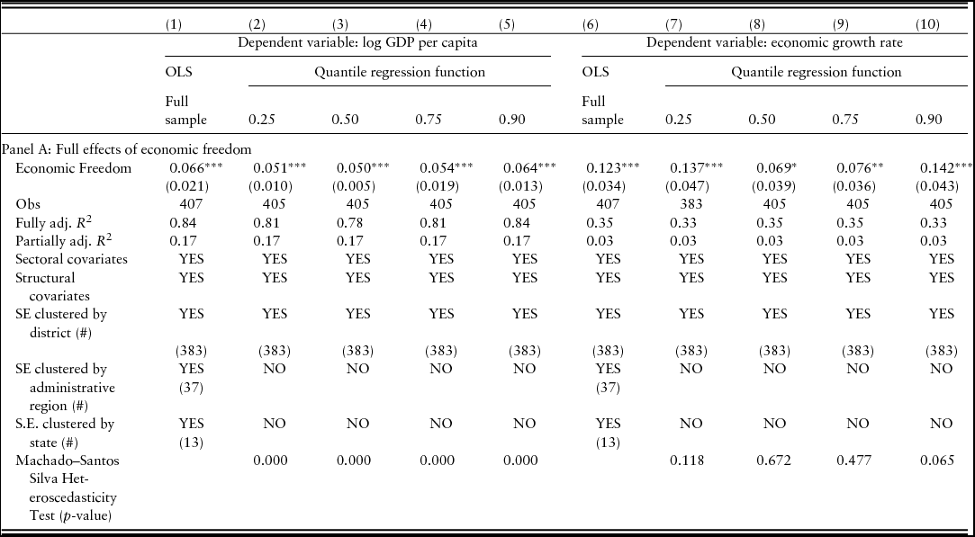
In Table 4, the quantile regression estimates of the underlying cross-district growth and income model specifications are presented. Columns (1) to (5) present the effects of economic freedom on income levels. In column (1), the full sample specification suggests that a 1 basis point improvement in the index of economic freedom is associated with a 6.6% increase in income level. In column (2), the effect of economic freedom on income level at the 25th percentile corresponds to the full sample OLS estimate with similar standard errors. In column (3), the effect at the median is slightly lower than at the 25th percentile. In column (4), the long-run effect of the economic freedom tends to rebound and recover the effect magnitude from the 25th percentile of the distribution. In column (5), the point estimate at the 90th percentile of the outcome distribution tends to increase by 10 basis points relative to the effect at the 75th percentile, and suggests that improving the level of economic freedom in the 90th percentile of district-level income distribution tends to boost per capita incomes in the respective percentile by 6.4%. Lower-income districts tend to gain disproportionately less from higher economic freedom than higher-income districts: the effect tends to weaken at the median, recover at the 75th percentile of the distribution, while it gains strength in the upper tail of the district-level per capita income distribution. Columns (6) to (10) present the short-run effect of economic freedom on district-level growth rates. In column (6), the full sample freedom growth estimate suggests that a 1 basis point improvement in the synthetic index of economic freedom is associated with a 12% improvement in the growth rate. Compared with its long-run counterpart, the short-run effect of economic freedom unveils substantial heterogeneity across various tails of the growth distribution. Column (7) reveals that improving economic freedom by 1 basis point in the 25th percentile of growth distribution is associated with a 13.7% expansion in short-run growth rate. The short-run effect tends to weaken substantially at the median of the growth distribution, as indicated by column (8). In column (9), the effect at the 75th percentile of the distribution is similar to the effect at the 25th percentile while the effect gains notable strength in column (10), which highlights considerable gains from greater economic freedom in the upper tail of growth distribution.
Effects of economic freedom on income level and growth rate across different quantiles of the outcomes

Notes: Table 4 presents the effects of economic freedom on real GDP per capita and its growth rate over time across different quantiles of each outcome. The standard errors are cluster-robust against the multiple spatial dimensions of heteroscedasticity and serially correlated stochastic disturbances using Machado and Santos Silva (2015) quantile regression function. Asterisks denote statistically significant regression coefficients at 10% (*), 5% (**) and 1% (***), respectively.
Counterfactual scenario
The ultimate question pertaining to the robustness of our estimates concerns the counterfactual scenario. Would German districts with below-average economic freedom significantly improve growth rates and income if they moved up the ladder of economic freedom? We construct a counterfactual scenario by focusing on the districts with a level of economic freedom on the synthetic index below the 90th percentile, to separate high-freedom districts from low-freedom ones. The level of economic freedom at the 90th percentile roughly corresponds to the level of economic freedom observed in the Landshut district in Lower Bavaria. Specifying the counterfactual threshold at the highest level of economic freedom observed in our sample is implausible, since an array of observable and idiosyncratic characteristics can be the driving force behind top level of economic freedom. Our counterfactual scenario invokes growth and income levels computed by using the point estimates from equations (3.1) and (3.2) in the following setup:
 $$\begin{eqnarray}
\ln y_{i \in \left\{ {1\left[ {EF < Q_{.90}^{EF}} \right]} \right\},j,k,l}^{\it Counterfactual} &=& \ln A + {{\hat{\gamma }}_1} \cdot EF_{j,k,l}^{Q\left( {.90} \right)} + {{\bf X^{\prime}}}\beta + \sum\limits_{j = 1}^J {{\hat{\phi }}_j} \cdot 1\left[ {i \in j} \right]\nonumber\\
&& +\, \sum\limits_{k = 1}^K {{{\hat{\alpha }}_k} \cdot 1\left[ {i \in j \in k} \right]} + \sum\limits_{l = 1}^L {{{\hat{\Theta }}_l} \cdot 1\left[ {i \in j \in k \in l} \right]}\quad
\end{eqnarray}$$
 $$\begin{eqnarray}
\Delta \ln y_{i \in \left\{ {1\left[ {EF < Q_{.90}^{EF}} \right]} \right\},j,k,l}^{\it Counterfactual} &=& \ln A + {{\hat{\lambda }}_1} \cdot EF_{j,k,l}^{Q\left( {.90} \right)} + {{\bf X^{\prime}}}\alpha + \sum\limits_{j = 1}^J {\mu _j} \cdot 1\left[ {i \in j} \right]\nonumber\\
&& +\, \sum\limits_{k = 1}^K {{\theta _k} \cdot 1\left[ {i \in j \in k} \right]} + \sum\limits_{l = 1}^L {{\Gamma _l} \cdot 1\left[ {i \in j \in k \in l} \right]}\quad
\end{eqnarray}$$
where ln yCounterfactual denotes the counterfactual level of income with the level of economic freedom at the 90th percentile, and Δln yCounterfactual is the equivalent counterfactual growth rate. The sample consists of the district-level observations below the 90th percentile economic freedom threshold, indicated by i ∈ {1[EF < QEF .90]}, j, k, l The vector X represents structural and sectoral covariates from the baseline regressions. Our benchmark specification used to construct the counterfactual scenario comprises the model specification with covariates, and standard errors clustered at the district, administrative unit, regional government and state levels to prevent serially correlated stochastic disturbances from undermining the inference on the two key parameters of interest,  ${\hat{\gamma }_1}$ and
 ${\hat{\lambda }_1}$. Using cross-district income and growth model specification, we obtain
 ${\hat{\gamma }_1} = .066$ (cluster-robust SE = 0.021) and
 ${\hat{\lambda }_1} = .123$ (cluster-robust S E = 0.034). The differences in economic freedom account for up to 17% of differences in income level across districts, and for up to 3% of differences in cross-district growth rates. We use the point estimates
 ${\hat{\lambda }_1}$ and
 ${\hat{\gamma }_1}$ to calculate the counterfactual district-level income and growth outcomes, taking into account the outcomes’ variance driven by the covariates.
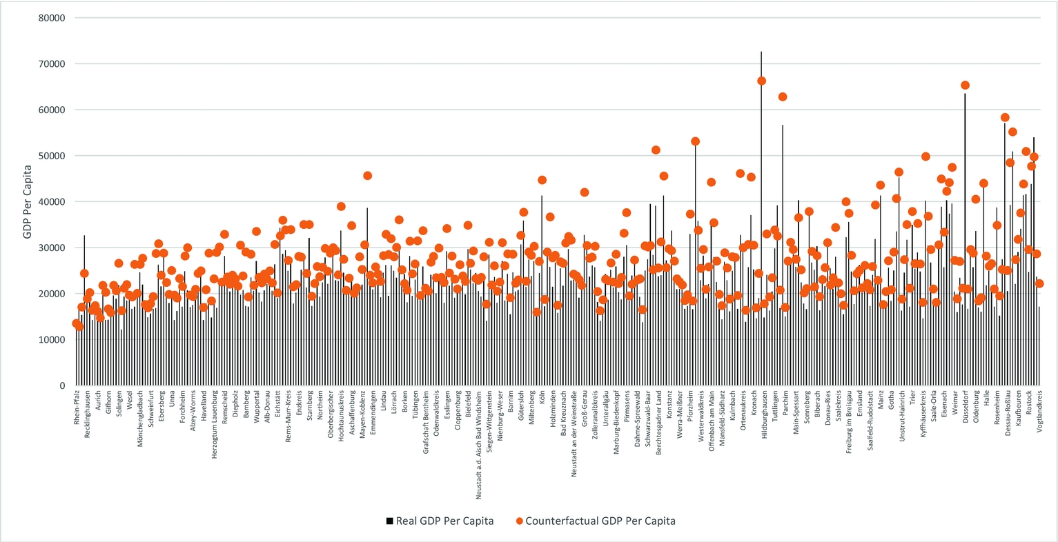
Figure 2 presents the counterfactual distribution of per capita income across districts. The transition to the 90th percentile of economic freedom is associated with marked income and growth gains. For districts characterized by low levels of economic freedom, the gains are remarkable. For Aachen district, the counterfactual scenario indicates a 55% increase in per capita income. Similarly, for the low-freedom districts Delmenhorst and Kaiserslautern, our counterfactual estimates indicate 45% and 41% improvements in per capita incomes. The counterfactual scenario suggests that the per capita income level is higher than the actual level in 89% of the below-90th percentile districts. The remaining 11% of districts are either characterized by exceptionally high income levels (München, Frankfurt am Main, Darmstadt) or display the counterfactual outcome very close to the actual level. The counterfactual Gini coefficient for the cross-district per capita income distributions drops by 4 basis points (from 0.19 to 0.15) suggesting that improving the level of economic freedom to the 90th percentile in below-cutoff districts tends to alleviate cross-district inequality.
Counterfactual GDP per capita with 90th percentile economic freedom.

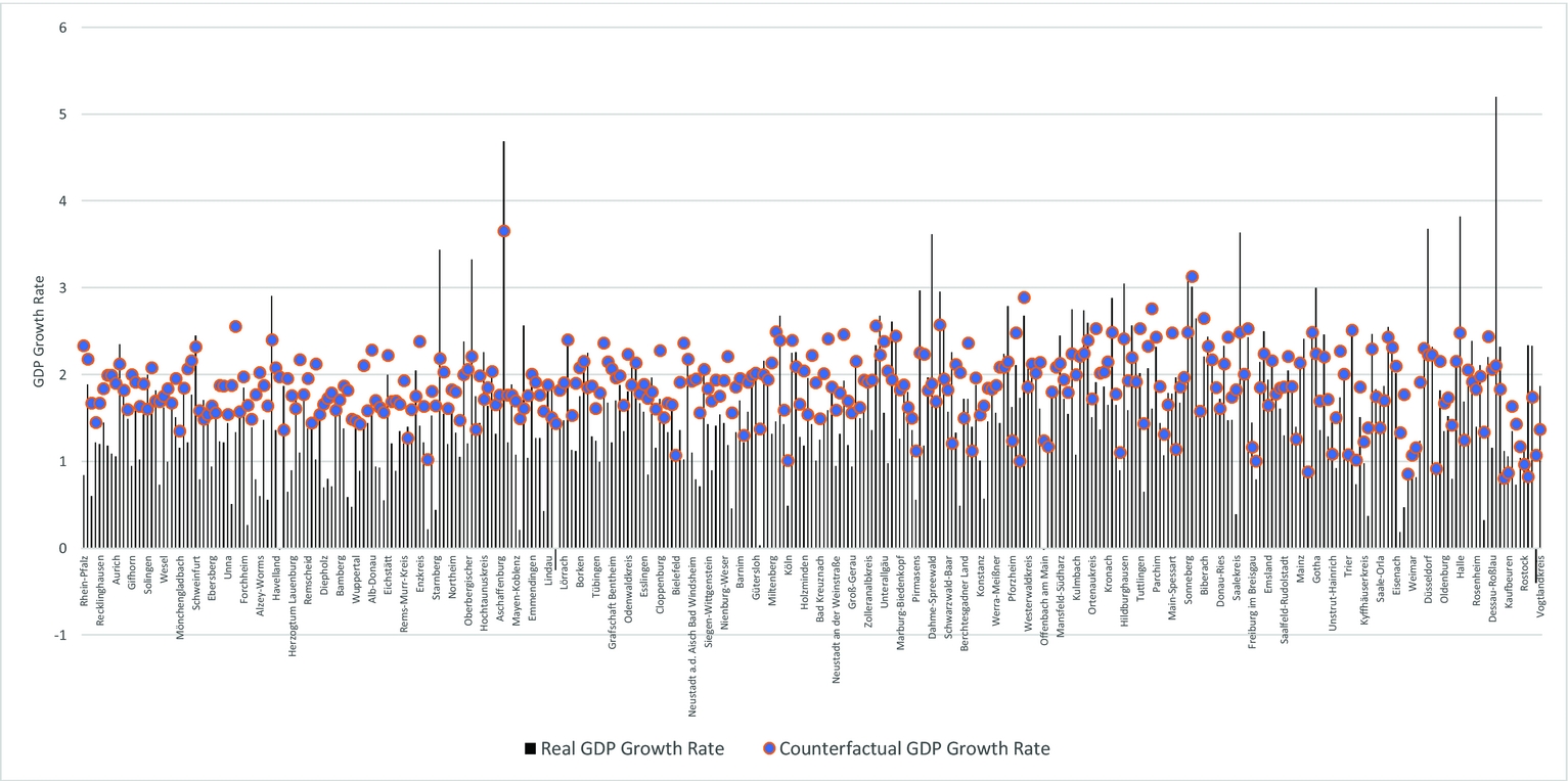
Figure 3 replicates the counterfactual scenario for the cross-district growth specification. The evidence unveils noticeable growth gains. About 65% of the districts tend to experience a higher rate of economic growth compared to the actual rate. The most substantial improvement is indicated for the districts Herne, Delmenhorst, Erzgebirgkreis and Leverkusen, where the growth rate gains at least 1.5 percentage points. The remaining third of the districts experience either exceptionally high rates of growth or the counterfactual rates as closely matched with the actual rates. The counterfactual outcomes highlight a notable decrease in cross-district growth inequality. The cross-district Gini coefficient on growth rates tends to drop by 20 percentage points, i.e. from 0.42 to 0.22.
Counterfactual growth rates with 90th percentile economic freedom.

From the normative perspective, the remaining question is what specific policy recommendation the counterfactual scenario could offer. The policy recommendation critically depends on the loading of eigenvectors in the synthetic index of economic freedom from section 2. The counterfactual scenario suggests that expanding economic freedom tends to reduce growth disparities and boost income levels across districts. Policies aimed at reducing the property tax burden and income tax rates and constraining public sector employment tend to have the most beneficial impact on expanding economic freedom, and are set to foster growth and income levels to the greatest degree. Policies aimed at reducing the business turnover taxes and public debt would tend to have a sizeable but moderate impact on economic freedom and growth, while the reduction of value-added taxes is set to influence economic freedom to the minimal degree. Nevertheless, reforms favouring lower property tax burden and lower individual income tax rates would yield a disproportionately favourable effect on growth and income levels compared to the other four components of economic freedom.
6. Conclusion
The notion that greater economic freedom is beneficial for growth and income levels has received widely acclaimed scholarly attention. However, most of the studies dealing with the relationship between economic freedom and growth establish such claims on the basis of cross-country variation in economic freedom and economic outcomes. The notion that economic freedom shapes economic growth and income levels in a common institutional environment is much less clear and warrants conclusive quantification at the subnational level.
In this paper, we revisit the relationship between economic freedom, per capita incomes and growth in a cross-section of 407 German districts for the period 1995–2010. We propose a new synthetic index of economic freedom consisting of ten different components capturing subnational variations in income and property taxation, public debt and public sector employment. The constructed synthetic index of economic freedom exhibits a substantial spatial variation across districts and rejects the traditional notion that former East German districts tend to suffer from the historical legacy of economic institutions that are not conducive to economic growth. The synthetic index reveals a reversal of the economic freedom pattern. Former East German and southern German districts tend to have markedly more economic freedom than their northern and western counterparts. Our analysis unveils a substantial and persistent north–south economic and institutional divide in the post-unification period.
Our results show that greater economic freedom fuels both short-run growth rate and long-run income levels. In our preferred specification, a 1 basis point improvement in the index of economic freedom is associated with an 8.5% increase in the growth rate, and with a 12.3% increase in income. The effect of economic freedom does not depend on the district-level sectoral structure, sample selection or geographic composition of the sample. In addition, the effect of economic freedom does not appear to be driven by outliers, and does not seem to be sensitive to the heterogeneity of the underlying relationship across various tails of the district-level per capita income- and growth distribution.
We further assess the potential economic gains of greater economic freedom and build a counterfactual scenario. The counterfactual scenario aims to examine the income and growth gains from greater economic freedom by moving districts with below-90th percentile-level economic freedom to the 90th percentile, and computing the hypothetical gains. The evidence clearly suggests that in the counterfactual scenario, per capita income level outperforms its actual counterpart in 89% of districts. The gains are noticeably stronger and quantitatively large in the districts at the bottom tail of the per capita income distribution. We also find that the counterfactual growth rates exceed the actual ones in more than two-thirds of districts, which testifies to the robust and beneficial effect of economic freedom on growth and income levels.
However, the origins of economic freedom under a common institutional environment in relation to the political, cultural and historical factors remain less clear. Such an enquiry might unravel the sources of institutional differences under a homogeneous institutional design and clearly comprises a promising research area to pursue in the future.
Acknowledgements
The authors would like to thank Dan Bogart, Bruno Gandlgruber, Simon Hartmann, Helena Helfer, Tobias Hlobil, Mitja Kovac, Matej Marinc, Vasja Rant, Pieter H. M. Ruys, Ivo Strejcek, Vesna Zabkar, the participants of Third WINIR Conference on Institutions and Human Behavior in Boston, the participants of the 2017 AEA Meeting in Chicago, and the participants of the 21st Annual SIOE Conference at Columbia University for their comments and feedback on the earlier draft version of the paper.