INTRODUCTION
Lentil (Lens culinaris Medik.) is an annual herbaceous, drought-tolerant legume best adapted to cool climates. The seeds of lentil are an important protein- and carbohydrate-rich food in many developing regions of West Asia, North Africa and many other areas of the world. Lentil is becoming increasingly popular in developed countries where they are perceived as a healthy component of the diet (Turk et al. Reference Turk, Tawaha and El-Shatnawi2003). Lentil is the second most stable cool season food legume (after chickpea) in Iran and the yield ranges from 457 to 774 kg/ha (Sabaghpour et al. Reference Sabaghpour, Safikhni, Sarker, Ghaffri and Ketata2004). Major production areas of lentil in Iran are found in west, northwest and northeast regions.
Lentil is adapted to less-favourable environments; it is predominantly grown in winter in the regions where annual average rainfall ranges between 300 and 400 mm (Sarker et al. Reference Sarker, Erskine and Singh2003). A short-season legume such as lentil, which could be planted early, would provide rotational benefits such as N fixation and increased surface soil stability, sufficient time for late summer rains to recharge the surface soil water for winter cereals establishment and alleviation of monoculture insect, disease and weed problems (Nielsen Reference Nielsen2001).
Lentil is grown in a wide-range of environments; hence, the yield of several genotypes tested across locations and over years differed due to high genotype by environment (G×E) interactions. The G×E interaction structure is an important aspect of both plant breeding programmes and the introductions of new crop cultivars. Understanding the causes of G×E interaction is important at all stages of plant breeding and can be used to establish breeding objectives, identify ideal test conditions and formulate recommendations for areas of optimal cultivar adaptation. Most breeders have used the term ‘stability’ to characterize a genotype which shows a relatively constant yield, independent of environmental conditions. This concept of stability is in agreement with the concept of homeostasis widely used in quantitative genetics (Becker & Leon Reference Becker and Leon1988) and may be considered as a ‘biological’ or ‘static’ concept of stability (Becker Reference Becker1981). A genotype showing a consistent performance in all environments does not necessarily respond to improved growing conditions (crop management) with increased yield. Agronomists, therefore, would prefer an ‘agronomic’ or ‘dynamic’ concept of stability (Becker Reference Becker1981; Becker & Leon Reference Becker and Leon1988) in which it is not required that the genotypic response to environmental conditions should be equal for all genotypes (Becker & Leon Reference Becker and Leon1988). Nassar & Huhn (Reference Nassar and Huhn1987) pointed out that the environmental variance is associated with the static or biological concept of stability. Lin & Binns (Reference Lin and Binns1988) proposed priority index (PI) as a measure of genotypic performance. Selection based on PI would favour selection for yield, as Kang & Pham (Reference Kang and Pham1991) found, and therefore involves a dynamic concept of stability.
Several statistical methods are available for analysis of adaptation, aimed at subdividing the information contained in a complex G×E interaction data matrix into simpler and more meaningful components representing real responses to genotypes and locations (the pattern) and a remainder possibly including only random variation (the noise; Gauch Reference Gauch1992). These range from univariate parametric models, such as regression slope (Finlay & Wilkinson Reference Finlay and Wilkinson1963) and environmental variance (Roemer 1917, cited by Becker Reference Becker1981), to multivariate models such as The additive main effect and multiplicative interaction (AMMI) analysis which was introduced by Gauch & Zobel (Reference Gauch and Zobel1988).
AMMI model is a hybrid model involving both additive and multiplicative components of two-way data structure. The model separates the additive variance from the multiplicative variance and then applies principal component analysis (PCA) to the interaction portion to a new set of coordinate axes that explains in more detail the interaction pattern and the estimation accomplished using the least squares principle. An F-test devised by Gollob (Reference Gollob1968) for the assessment of PC axes proved too liberal both on theoretical grounds and following simulation results. The AMMI analysis has been shown to be effective because it captures a large portion of the G×E sum of squares, clearly separating main and interaction effects that present agricultural researchers with different kinds of opportunities, and the model often provides an agronomically meaningful interpretation of the data (Gauch Reference Gauch1992).
The concept of stability for agriculture was recognized by Roemer (1917, cited by Flores et al. Reference Flores, Moreno and Cubero1998), who used the variance across environments for yield stability. Applied to a certain genotype, it is a biological concept. Lin & Binns (Reference Lin and Binns1988) defined the PI parameter as a genotype's general superiority and defined it as the distance mean square between the genotype's response and the maximum response over locations. PI satisfies the agronomic concept of stability.
The objectives of the present work have been: (i) to compare, using seven different measures of the AMMI model, environmental variance and PI statistics, the stability and adaptability of improved lentil genotypes for grain yield, and (ii) to explore the advantages and disadvantages of each AMMI measure in selecting more stable or better-adapted lentil genotypes based on static and dynamic concepts of stability.
MATERIALS AND METHODS
Plant material
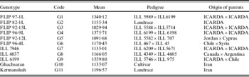
Eleven lentil genotypes were used, including one Iranian commercial variety (Ghachsaran), one Iranian local landrace (Kermanshah) and nine advanced lines from the lentil breeding programme of ICARDA. Descriptions of genotypes and some details are given in Table 1.
The characterization of 11 lentil genotypes studied in multi-environmental trials

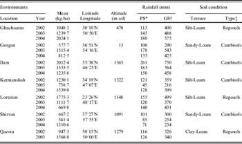
The trials were conducted at seven rainfed Field Crops Stations in Iran over 3 years (2002–04), except for Qazvin Field Crops Station where experiments were conducted over 2 years (2002–03). The detailed description of these test stations is given in Table 2.
The environmental characterization of lentil multi-environmental trials

* Preseasonal rainfall.
† Growing season includes months from Feb to Apr.
‡ According to FAO system of soil classification.
The experimental layout was a randomized complete block design (RCBD) with four replications in each trial. Trials were planted according to local practices of each location. Management and fertilization at each location were carried out according to practices of each Field Crops Station. Fertilization rates with planting were inflated by about 10% to insure good and even stands (crop establishment in field) and development.
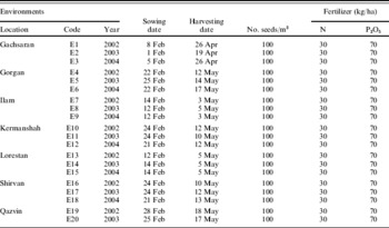
The plot size was 4 m2 (4 m long containing 4 rows spaced 0·25 m apart). The plant density was 100 plants m2 with a plant-to-plant distance of 40 mm (25 seeds for each 1 m row). Sowing depth was 35 mm and it was done manually. The introduced genotype Ghachsaran and local landrace Kermanshah were used as standard control genotypes. Planting was carried out following the optimal dates for each location (Table 3) and all the recommended agronomic practices. Fertilizer application was 30 kg N/ha and 70 kg P2O5/ha at planting stage. No irrigation was carried out. Weeds were culled by hand as required. Evaluations were conducted for several agronomic traits, but complete data were obtained only for grain yield in all the location–year combinations, hereafter referred to as environments. The value of grain yield was determined from the two central rows of each plot (the area harvested was 1·75 m2) and expressed in kg/ha.
Local agronomic practices of testing environments in Iran

Statistical analysis
An analysis of variance (ANOVA) was performed for each environment separately as an RCBD (data and results not presented). A combined ANOVA was undertaken over all environments. The environments were considered as random variables while the genotypes were treated as fixed variables. All analyses were performed using the statistical package GENSTAT release 7.1 (GENSTAT 2004) for AMMI's ANOVA and SAS release 6.12 (SAS Institute 1996) for AMMI's parameters and other stability statistics. Bartlett's test was used to determine the homogeneity of variances between environments to determine the validity of the combined ANOVA on the data.
Different methods of data analysis were used to investigate G×E interactions for total grain yields. AMMI combines ANOVA into a single model with additive and multiplicative parameters. The model equation is:

where Y ij is the yield of the ith genotype in the jth environment; μ is the grand mean; g i and e j are the genotype and environment deviations from the grand mean, respectively; λn is the eigenvalue of the PC analysis axis n; γin and δjn are the genotype and environment principal component scores (eigenvectors) for axis n; n is the number of principal components retained in the model and ρij is the error term.
The AMMI model does not make provision for a quantitative stability measure; however, such measures are essential in order to quantify and rank genotypes according their yield stability. The following measures have been proposed by different researchers. Zobel (Reference Zobel1994) suggested the two AMMI stability measures (EV1 and EVF) as averages of the squared eigenvector values. The equation for the EV parameter is written as:

where N=1 for EV1. For EVF, N was the number of PC that were retained in the AMMI procedure via F-tests. Genotypes with low values of EVs have smaller fluctuations across environments and therefore are more stable.
The next two AMMI measures (AMGE1 and AMGEF) are the sum across environments of the G×E interaction modelled by AMMI procedure (Sneller et al. Reference Sneller, Cilgore-Norquest and Dombek1997). These parameters are expressed as:

where M is the number of environments; for AMGE1, N was one, for AMGEF N was the number of PC that were retained in the AMMI procedure via F-tests. The genotypes with the lowest AMGE1 and AMGEF values are considered the most stable.
The PC scores of a genotype in the AMMI analysis are an indication of the stability of a genotype over environments. The lower the PC scores, either negative or positive (as it is a relative value), the more stable a genotype is to environments. Therefore, the next two AMMI statistics (SIPC1 and SIPCF) are sums of the absolute value of the interaction principal component (IPC) scores for the ith genotype: for SIPC1, N was one; for SIPCF, N was the number of IPCs that were retained in the AMMI model via F-tests.

The genotypes with lower SIPCs (SIPC1 and SIPCF) values are considered more stable (Sneller et al. Reference Sneller, Cilgore-Norquest and Dombek1997). In Eqn (4), N=1 for SIPC1; for SIPCF N was the number of PC that were retained in the AMMI procedure via F-tests. The genotypes with lower SIPC (SIPC1 and SIPCF) values are considered more stable. AMMI's stability value (ASV) was calculated using the following formula, as suggested by Purchase (Reference Purchase1997).

where ASV=AMMI's stability value, SS=sum of squares, PC1=interaction of PCA one and PC2=interaction of PCA two. The genotypes with the highest ASV values are considered the most stable. For determining static (biological) and dynamic (agronomical) concepts of stability of motioned AMMI stability measures, used environmental variance (Roemer 1917 in Flores et al. Reference Flores, Moreno and Cubero1998) and PI (Lin & Binns Reference Lin and Binns1988).
RESULTS
Analysis of variance
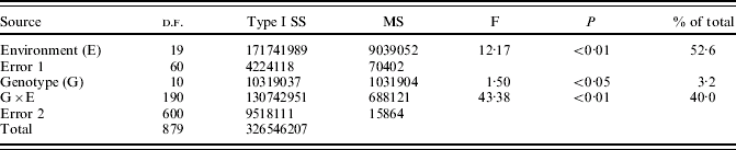
Bartlett's test suggested (χ2=28·2, P<0·05) that error variances were homogeneous. The combined ANOVA showed that genotypes (G) differed significantly (P<0·01) in mean yields (Table 4). Environments (E) were significantly (P<0·01) different. Genotype by environment (G×E) interactions were also significant (P<0·01). The significance of G×E interaction effects demonstrated that genotypes responded differently to variations in environmental conditions. These variations could be attributed to different climatic conditions for different years and locations and to different edaphic conditions at different locations (Table 2).
ANOVA of lentil performance trial yield data
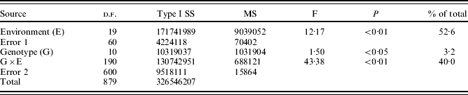
The ANOVA also showed that out of the total sum of squares, 53, 3 and 40% was attributable to E, G and G×E interaction effects, respectively (Table 4). The large proportion of variation due to environment did not, however, reduce the importance of the differences due to genotypes or G×E interactions. The size of genotype sum of squares in relation to the G×E sum of squares indicated substantial differences in genotype response in different environments.
Stability analysis
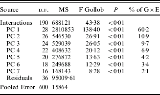
ANOVA for AMMI
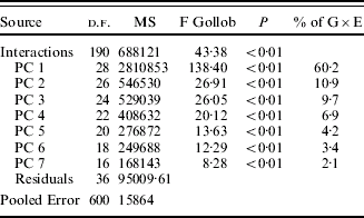
The G×E interaction was further analysed with the aid of the AMMI model for grain yield stability. The AMMI model including PC1 and PC2 accounted for 11–60% of the G×E variation of grain yield in studied lentil genotypes. Table 5 shows the seven PC axes declared significant by the F-test that was proposed by Gollob (Reference Gollob1968). Although the first PC axis of G×E interaction accounted for 60% of G×E interaction sum of squares, the seven PCs retained by Gollob's F-test accounted for 97% of G×E interaction sum of squares. The AMMI model used in the present research exhibited a more complex interaction, but retained only two PCs for interpretations since these account for a substantial amount, 71%, of G×E interaction sum of squares and can facilitate graphical visualization of the genotypes in low dimensions.
AMMI analysis of grain yield, with 20 environments and 11 lentil genotypes
Common stability parameters
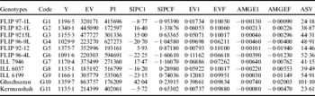
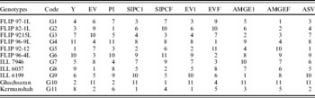
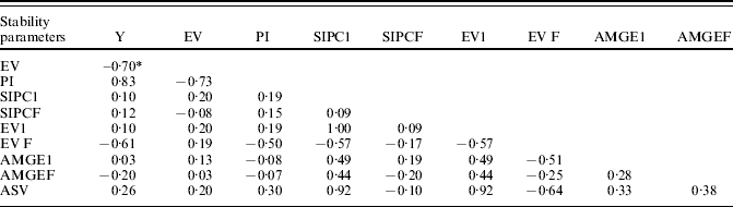
Table 6 shows results for stability of different lentil genotypes according to environmental variance (Roemer 1917 in Flores et al. Reference Flores, Moreno and Cubero1998), PI (Lin & Binns Reference Lin and Binns1988) and seven AMMI stability measures. The ranks of lentil genotypes based on these stability parameters are given in Table 7. According to the environmental variance (EV) stability statistic, a genotype is considered to be more stable provided that the EV is lower. Therefore, genotype G8 (ILL 6037) was the most stable genotype and had biological stability whereas genotype G10 (Ghachsaran) was the least stable of those which had high mean yield performance. Since EV does not provide any advantage in favourable environments, genotypes screened by this measure can be recommended for less-favourable environments or where farmers do not have advanced technology. EV showed significant negative rank correlation with mean yield and PI parameter, but did not show any significant rank correlation with AMMIs procedure parameters (Table 8).
Mean yields in kg/ha (Y) and stability parameter estimates (EV, PI and seven AMMI stability statistics) for lentil yields of 11 genotypes tested in 20 environments

Ranks 11 lentil genotypes according to mean yields (Y) and stability parameters (EV, PI and seven AMMI stability statistics)

Spearman's correlation coefficients among ranks of 11 lentil genotypes at 20 environments

* Critical values of correlation P<0·05 and P<0·01 (d.f. 9) are 0·602 and 0·735, respectively.
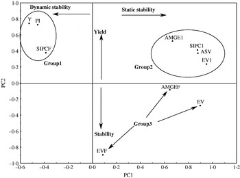
As a stability statistic, the genotype PI of Lin & Binns (Reference Lin and Binns1988) is estimated by the square of differences between a given genotype and the maximum genotype mean at a location, summed and divided by twice the number of locations. The genotypes with the lowest PI values are considered the most stable. Table 6 presents the genotype performance measure PI for grain yield of the 11 lentil genotypes tested in 20 environments. From this analysis, the most stable genotype ranked first for PI values was genotype G2 (FLIP 82-1L) followed by G10, ranked second for PI and for mean yield. Others with low PI values were G4 (FLIP 96-9L) followed by genotype G6 (FLIP 96-4L). The ranks of the PI measure and mean yield are relatively in agreement (Table 6) and indicate that the PI measure is more an indication of performance and not really an indication of stability. PI showed significant positive rank correlation with mean yield, significant negative rank correlation with EV, but did not show any significant rank correlation with AMMI's procedure parameters (Table 8). Lin & Binns (Reference Lin and Binns1988) proposed PI as a measure of genotypic performance, in a possible attempt to integrate both yield and stability. Figure 1 shows that PI is strongly related with mean yield. Selection based on this method (PI) would favour selection for yield, as Kang & Pham (Reference Kang and Pham1991) and Flores et al. (Reference Flores, Moreno and Cubero1998) found. The most unstable genotypes according to this analysis were G4 followed by G6, which are also low-yielding genotypes (Table 6).
Plot of the first two principal components (PC1 v. PC2) of standard values of stability of yield, estimated by nine methods using yield data from 11 lentil genotypes grown in 20 environments.

Stability parameters of AMMI
The values of the SIPC1 statistic for each genotype could be useful in identifying its stability in AMMI procedure. The local genotype G11 (Kermanshah) had the lowest absolute value of this statistic and so can be considered as the most stable genotype. The second rank of SIPC1 belonged to genotype G5 (FLIP 92-12L), which had the high mean yield. The least stable genotypes according to SIPC1 were G10 and G9 (ILL 6199). G10 had the highest mean yield and is registered as commercial cultivar. The SIPC1 showed significant positive rank correlation with ASV and EV1 parameters, but did not show significant rank correlation with mean yield and other stability statistics (Table 8). SIPCF stability parameter values and the stability ranking as well as mean yield with its ranking are given in Tables 5 and 6. The most stable genotypes indicated by this stability parameter were G10 and G8 (ILL6037). The genotypes with poor stability according to SIPCF were G6 and G2, with G2 being ranked third for mean yield. Therefore, the more stable genotypes of SIPCF stability parameter did not have high yield performance and showed a static concept of stability. This parameter was not correlated (either positively or negatively) with other parameters (Table 8).
The results of the EV1 stability statistic are given in Table 6; the most stable genotypes were the local genotypes G11 and G5, with G5 being ranked highest for mean yield. The most unstable genotypes according to the EV1 method were G10 and G9. The most stable and unstable genotypes based on the EV1 method were very similar to the SIPC1 procedure. This indicates that these two procedures are equivalent for ranking genotypes and identifying the most stable and unstable cultivars. The EV1 statistic showed significant positive rank correlation with ASV and SIPC1 parameters, but did not show significant rank correlation with genotypes mean yield and other stability parameters (Table 8). According to the EVF procedure, G4 and G6 were the most stable genotypes, with G5 and G2 the most unstable. Both G5 and G2 were significantly higher yielding than the other genotypes. However, EVF seems to be representing the biological (dynamic) concept of stability. It indicated significant negative rank correlation with ASV and mean yield, but did not show any significant rank correlation with other stability statistics (Table 8).
The AMMI statistics AMGEs (AMGE1 and AMGEF) are the sum of eigenvectors across all studied environments (Sneller et al. Reference Sneller, Cilgore-Norquest and Dombek1997). The largest absolute values of AMGE1 were for genotypes G10 and G7 (ILL 7946), therefore these genotypes are considered the least stable genotypes. The most stable genotypes of this method were G9 and G3 (FLIP 92-15L), which had minimum absolute values of this statistic and showing rank correlation with EV. The smallest absolute value for the AMGEF parameter were for G1 (FLIP 97-1L), G2 and G3 (the most stable genotypes according to this parameter) and they were close to minimum amounts, while the genotypes G5 and G10 had the largest absolute values of AMGEF and therefore were the least stable. These genotypes had the highest mean yield performance. The AMGE1 and AMGEF statistics of AMMI model introduced the high mean yield genotypes (G5 and G10) as the least stable genotypes and therefore showed biological stability (Lin et al. Reference Lin, C.S., Binns and Lefkovitch1986). The AMGE1 and AMGEF statistics were not correlated (either positively or negatively) with other parameters and mean yield (Table 8).
The ASV as described by Purchase (Reference Purchase1997) is comparable with the other stability parameters of AMMI model and other methods of stability such as EV (Roemer 1917, cited by Flores et al. Reference Flores, Moreno and Cubero1998) and PI (Lin & Binns Reference Lin and Binns1988) in the study of G×E interaction. Table 6 indicates the ASV values of the AMMI model for each genotype and also their ranking for the 11 lentil genotypes. According to the ASV ranking, genotype G5 and local control genotype G11 were the most stable. The most unstable were G10 and G9. ASV was reported to produce a balanced measurement between the two first PC's (PC1 and PC2) scores (Purchase Reference Purchase1997). The ASV showed significant positive rank correlation with SIPC1 and EV1 parameters, but showed significant negative rank correlation with EVF statistic (Table 8).
Visualization of association among different stability parameters
Each of the methods produced a quantitative value for each genotype (Table 6). The correlation matrix was calculated and a PCA based on this correlation matrix was performed on a set of lentil stability data. There are many statistical methods for stability analyses; AMMI stability statistics have been compared and two different concepts of stability (static and dynamic) have been suggested. The first two PCs (PC1 and PC2) of standard values of different stability procedures accounted for 73% (46 and 26% PC1 and PC2, respectively) of the variance of the original variables. Figure 1 shows that the first PC (PC1) separates the methods PI, SIPCF and means yield (Y) from the other methods. Kang & Pham (Reference Kang and Pham1991) pointed out that the PI is strongly related with high mean yield and involves an agronomic concept of stability. Thus, the PC1 separates the methods into two groups according to the two stability concepts, being similar to the findings of Flores et al. (Reference Flores, Moreno and Cubero1998). Figure 1 shows, on the right, methods corresponding to the biological concept and, on the left, the methods based on the agronomic concept of stability. The PC2 splits the scatter into three groups. The mean yield (Y) is included in Group 1 with PI and SIPCF parameters, suggesting Group 1 comprises those methods where yield has an important influence on the ranking across environments.
Group 2 includes the EV1, SIPC1, AMGE1 and ASV parameters and Group 3 includes the EVF and AMGEF parameters, which are strongly correlated with EV. Group 2 is intermediate between Groups 1 and 3 and consists of methods that are influenced simultaneously by both yield and stability.
DISCUSSION
In the present study, partitioning and interpretation of the G×E interaction was based on the AMMI stability technique (Zobel et al. Reference Zobel, Wright and Gauch1988) and two former procedures for G×E interaction analysis (EV and PI). The former method (univariate analysis) had shown certain deficiencies for determining and explaining G×E interaction patterns and they attempt to define the G×E interactions by one parameter; however the multiplicative G×E interaction component is far too complex to be summarized by one parameter. Multivariate statistical methods such as AMMI have been introduced to explore multidirectionality aspects and attempt to extract more information from this component. The present dataset and other similar studies (Nachit et al. Reference Nachit, Nachit, Ketata, Gauch and Zobel1992) encountered problems, because these techniques confound interaction and main effects (Wright Reference Wright1971) and are unable to explain non-linear genotypic response to the environments. In contrast, AMMI analysis appears to be able to extract a large portion of the G×E interaction and is thus more efficient in analysing G×E interaction pattern in different crops such as cereals (maize), legumes (lentil), and oilseeds (soybean), as demonstrated by Zobel et al. (Reference Zobel, Wright and Gauch1988). The AMMI analysis does not make provision for a stability parameter; such measures, proposed by different researchers, are essential in order to quantify genotypes' yield stability (Zobel et al. Reference Zobel, Wright and Gauch1988; Purchase Reference Purchase1997; Sneller et al. Reference Sneller, Cilgore-Norquest and Dombek1997).
Traditionally, most breeders since Roemer (1917, cited by Flores et al. Reference Flores, Moreno and Cubero1998) have used the term stability to characterize a genotype which shows a relatively constant yield, independent of environmental conditions. This concept of stability is in agreement with the concept of homeostasis widely used in quantitative genetics and may be considered as a biological or static concept of stability (Becker & Leon Reference Becker and Leon1988). This type of stability is not acceptable to most breeders, who would prefer an agronomic or dynamic concept of stability. In the dynamic concept of stability, it is not required that the genotypic response to environmental conditions should be equal for all genotypes (Becker Reference Becker1981). Yield stability depends on yield components and other plant characteristics, such as tolerance to environmental stress factors, e.g. drought conditions. Reductions in lentil yields in a rainfed culture are chiefly observed after a preseason drought, particularly if the season is also dry. Location means varied with different soil and climatic conditions and they also appeared to respond positively to increased rainfall, although these differences could not be tested (Table 2). Like the results obtained from AMMI models used in soybean MET (Zobel et al. Reference Zobel, Wright and Gauch1988), the AMMI model used in the present research exhibited a more complex interaction which required as many as seven PCs, but the first two PCs accounted for a considerable amount of variation in the G×E interaction. This could be associated with the nature of the crop, environmental conditions or diverse genetic background obtained from different sources.
The AMMI analysis provided a better description of static and dynamic concepts of stability for interpreting G×E interaction. Stability methods clearly influenced by high mean yield are the PI and SIPCF AMMI parameters. In the present case, both the methods are grouped close to each other in Group 1 and, as already mentioned by Flores (Reference Flores1993), G×E interaction effects were overshadowed by genetic effects. However, these methods are influenced by both high mean yield and stability simultaneously and selection for the most stable genotypes according to these procedures results in the high performance genotypes being introduced as the most stable genotypes.
Simultaneous assessment of PC scores of the AMMI method for lentil genotypes facilitates the interpretation and identification of superior genotypes among them. For example, genotypes with a low PC would be more stable (Gauch Reference Gauch1992). AMMI has been also useful for determining the concept and nature of stability and G×E interaction for grain yield. The methods comprising Group 2 are EV1, SIPC1, AMGE1 and ASV parameters. Adugna & Labuschagne (Reference Adugna and Labuschagne2002) found that the ASV parameter of the AMMI method would be a useful tool for simultaneously selecting for yield and yield stability, although it associated is with EV and represents static stability. Finally, the methods in Group 3 share a common feature: all of them measure only stability. These methods are EVF and AMGEF parameters of the AMMI model and EV of Roemer (1917 in Flores et al. Reference Flores, Moreno and Cubero1998). As Flores et al. (Reference Flores, Moreno and Cubero1998) suggested, the approach of EV is similar to that of EVF and AMGEF parameters of AMMI model in attempting to determine the static or biological concept of stability.
The present research demonstrated the advantage of adding the AMMI model and its parameters for the analysis of the G×E for grain yield in lentil. The present findings do not allow to be widely recommended for assessing G×E interactions. However, the AMMI analysis and its stability statistics appear particularly useful for depicting static and dynamic responses of legumes and especially lentil grain over the entire lentil-producing areas of Iran. In conclusion, several of the stability statistics that have been employed in the present study quantified stability of genotypes with or with no respect to yield. Both yield and stability of performance should be considered simultaneously to exploit the useful effects of G×E interaction and to make selection of the genotypes more precise and refined. Despite the fact that the different stability statistics are indicative of high-, intermediate-, or low-stability performance, the SIPCF do not provide information for reaching definitive conclusions. Therefore, the ASV statistic is indispensable, as farmers would prefer to use a high-yielding genotype that performs consistently from year to year. Thus, the best recommended genotype according to the present study is G5 (FLIP 92-12), which had high mean yield and was the most stable based on ASV. Selection of genotypes for stability is needed in most dry-land environments, where the environment is variable and unpredictable. Therefore, genotype evaluation under variable environments and adoption of simultaneous selection for yield and stability is the most valuable selection index that can be used in any plant breeding programme. Finally, the following findings can be summarized from the present study: (1) G5 (FLIP 92-12) was found to be the most stable genotype and is thus recommended for commercial release; (2) the ASV statistic of the AMMI model was found to be useful in detecting the phenotypic stability of the genotypes studied; and (3) the significant G×E interactions and the changes in ranks of genotypes across environments suggest a breeding strategy of specifically adapted genotypes in homogeneously grouped environments.
The authors thank the Iranian Dry Agricultural Research Organization for making available the plant materials, experimental locations and technical assistance. We thank two anonymous reviewers of the Journal Agricultural Science, Cambridge for their helpful comments, suggestions and corrections of the manuscript.