1 Introduction
Shock wave boundary layer interactions (SWBLI) occur in many parts of aircraft such as wings, control surfaces, intakes and other components that can affect the performance of the aircraft. Many theoretical, numerical and experimental investigations have been conducted to fully understand the phenomenon of SWBLI for more than half a century. Especially well-known studies, which have contributed to our theoretical understanding of this problem, are by Lighthill (Reference Lighthill1953), Gadd (Reference Gadd1957), Chapman, Kuehn & Larson (Reference Chapman, Kuehn and Larson1958), Brown & Stewartson (Reference Brown and Stewartson1969), Neiland (Reference Neiland1969), Stewartson & Williams (Reference Stewartson and Williams1969), Messiter (Reference Messiter1970), Neiland (Reference Neiland1970) and Neiland (Reference Neiland1973). The major advances in understanding laminar SWBLI and separation were made by Brown & Stewartson (Reference Brown and Stewartson1969), Neiland (Reference Neiland1969), Stewartson & Williams (Reference Stewartson and Williams1969) and Neiland (Reference Neiland1970).
It was Prandtl (Reference Prandtl1904) who first showed that a fluid in motion comes to rest at the surface within a thin viscous layer, termed a boundary layer, which responds to pressure perturbations in the external flow. If this disturbance is strong enough, it can provoke separation. In Prandtl’s theory, the fluid motion is described using a hierarchical order which begins from a known pressure in the outer inviscid flow and then used to iteratively solve for the lower viscous layer.
The phenomenon of boundary layer separation is a critical feature when the fluid flowing past a surface encounters a severe pressure gradient. In such a circumstance, the boundary layer thickness can abruptly change from
 $O(Re^{-1/2})$
upstream of separation to
 $O(1)$
downstream of separation. Here,
 $Re$
is a characteristically large Reynolds number. When separation occurs, Prandtl boundary layer equations cease to be valid. The possibility of a singularity under these conditions was first noted and studied by Goldstein (Reference Goldstein1948). Studies of boundary layer separation in incompressible and compressible flows have since been made using the asymptotic theory valid in the limit of infinite Reynolds number. According to Goldstein’s theory, singularity at separation is associated with singularity in the displacement thickness of the boundary layer. Later Catherall & Mangler (Reference Catherall and Mangler1966) showed that separation can be regular provided the displacement thickness is directly and intimately related to the pressure gradient. Such situations usually arise in shock wave–boundary layer interactions. Cathrall & Mangler’s paper gave impetus to many papers in the 1970s, 1980s and 1990s on interactive boundary layers and separation such as those by Werle & Vasta (Reference Werle and Vasta1974), Le Balleur (Reference Le Balleur1977), Le Balleur (Reference Le Balleur1978), Veldman (Reference Veldman1979), Burggraf et al. (Reference Burggraf, Rizzetta, Werle and Vatsa1979), Veldman (Reference Veldman1980) and Coenen (Reference Coenen1999).
Neiland (Reference Neiland1969), Stewartson & Williams (Reference Stewartson and Williams1969), Messiter (Reference Messiter1970) and Sychev (Reference Sychev1972) also introduced the triple-deck theory to resolve the problem of separation based on an asymptotic approach of the Navier–Stokes equations. The theory assumes that, in the vicinity of separation, perturbations thicken the boundary layer which breaks into three distinct regions. The first, near the wall, is a rotational viscous subsonic region which is most sensitive to disturbances, the second is a main inviscid rotational region and the third is an inviscid irrotational outer region, which is most resistive to disturbances. Interaction between these decks (Stewartson Reference Stewartson1974) has been shown to be dependent on wall temperature by a number of authors such as Brown, Cheng & Lee (Reference Brown, Cheng and Lee1990), Seddougui, Bowles & Smith (Reference Seddougui, Bowles and Smith1991), Kerimbekov, Ruban & Walker (Reference Kerimbekov, Ruban and Walker1994), Cassel, Ruban & Walker (Reference Cassel, Ruban and Walker1995), Cassel, Ruban & Walker (Reference Cassel, Ruban and Walker1996), Neiland, Sokolov & Shvedchenko (Reference Neiland, Sokolov and Shvedchenko2009) and Shvedchenko (Reference Shvedchenko2009).
The problem of leading edge separation, on the other hand, was first discussed by Chapman et al. (Reference Chapman, Kuehn and Larson1958) because it lent itself particularly well for the development of their isentropic recompression theory. The theory helped predict base pressures and drag with the use of a simple relation (see Chapman et al. Reference Chapman, Kuehn and Larson1958). The rationale behind such geometry is that it is simple because it precludes the effect of a pre-existing boundary layer and allowed Chapman’s already-existing laminar mixing layer theory be used to predict the dead air pressure in a separated region. Another justification for the geometry is from a fundamental point of view. Leading edge separation is a limiting case of more practical examples such as base flows, compression corners and steps wherein the distance from the leading edge to the separation point is reduced to zero, and wherein the separated region becomes quite large compared to the other geometries. Beyond the study of Chapman and his associates, however, leading edge separation has not been widely considered except by Stewartson (Reference Stewartson1964) and Brown & Stewartson (Reference Brown and Stewartson1969), who briefly mentioned that it is worth exploring from a more rigorous standpoint. It should also be mentioned that Chapman et al. (Reference Chapman, Kuehn and Larson1958) restricted their investigation to moderate supersonic Mach numbers and high Reynolds numbers. This, as a result, makes viscous-dominated flow conditions (of high Mach numbers and low Reynolds numbers) encountered in hypersonic flight of particular interest for research.
Leading edge separation, in recent years, has been studied by the hypersonic group at the University of New South Wales computationally, experimentally and analytically. In the study by Khraibut et al. (Reference Khraibut, Gai, Brown and Neely2017) wall temperature effects on a two-dimensional steady hypersonic laminar leading edge separation were considered. In this paper, we give special emphasis to bluntness effects on the leading edge separation. Bluntness effects are critical in hypersonic flight mainly from a vehicle design viewpoint because they influence the thermal loads on a vehicle (Hirschel Reference Hirschel2005), onset of boundary layer transition and instabilities in the flow (e.g. Brinich Reference Brinich1956; Softley Reference Softley1969; Gray & Rhudy Reference Gray and Rhudy1972; Stetson Reference Stetson1978; Dietz & Meijering Reference Dietz and Meijering1997). Bluntness, furthermore, is critical from a practical point of view because the leading edge design is typically restricted by manufacturing limitations imposing a finite thickness on the leading edge.
Earlier studies in the 1950s, 1960s and 1970s mainly dealt with bluntness effects on flow transition (Moeckel Reference Moeckel1957; Nagamatsu, Graber & Sheer Reference Nagamatsu, Graber and Sheer1966; Softley Reference Softley1969; Pate Reference Pate1977; Stetson Reference Stetson1978), SWBLI (Bertram Reference Bertram1954; Bertram & Henderson Jr Reference Bertram and Henderson1958; Cheng et al. Reference Cheng, Hall, Golian and Hertzberg1961; Holloway, Sterrett & Creekmore Reference Holloway, Sterrett and Creekmore1965; Holden Reference Holden1966; Townsend Reference Townsend1966; Edney Reference Edney1968; Edwards & Anders Reference Edwards and Anders1968; Holden Reference Holden1971; Gray & Rhudy Reference Gray and Rhudy1972) or the combined effect of bluntness and incidence angle (Bertram & Henderson Jr Reference Bertram and Henderson1958; Creager Reference Creager1959; Cheng et al. Reference Cheng, Hall, Golian and Hertzberg1961; Nagamatsu et al. Reference Nagamatsu, Graber and Sheer1966; Kemp Reference Kemp1969; Stetson Reference Stetson1978). The importance of bluntness effects on hypersonic separations can also be seen, in particular, when noting that many studies have returned to the subject in recent years, such as those by Mason & Lee (Reference Mason and Lee1994), Khorrami & Smith (Reference Khorrami and Smith1994), Mallinson, Gai & Mudford (Reference Mallinson, Gai and Mudford1996), Marini (Reference Marini1998), Santos (Reference Santos2005), Borovoy, Skuratov & Struminskaya (Reference Borovoy, Skuratov and Struminskaya2008), Borovoy et al. (Reference Borovoy, Mosharov, Radchenko, Skuratov and Struminskaya2014) and John & Kulkarni (Reference John and Kulkarni2014).
Effects of bluntness in low-density flows were also investigated numerically by Santos (Reference Santos2005) and experimentally by Edwards & Anders (Reference Edwards and Anders1968). In the experimental studies of Edwards & Anders (Reference Edwards and Anders1968), they observed an increase in the extent of separation with increasing bluntness in a compression-ramp geometry. Townsend (Reference Townsend1966), who also investigated the effect of bluntness on a compression-ramp experimentally, found bluntness effects on separation to be caused by the boundary layer’s outer edge flow conditions at the beginning of the interaction, where the pressure is just about to rise.
It should be noted here that Lees & Probstein (Reference Lees and Probstein1952) were the first to relate the pressure rise caused by boundary layer growth to hypersonic viscous interaction parameter
 $\bar{\unicode[STIX]{x1D712}}=M^{3}(C/Re)^{1/2}$
, where
 $M$
is the Mach number,
 $Re$
is the Reynolds number and
 $C$
is the Chapman–Rubesin constant. Cheng & Pallone (Reference Cheng and Pallone1956) then extended the work of Lees & Probstein (Reference Lees and Probstein1952) to flat plates with blunt leading edge, based mainly on the blast wave theory of Taylor (Reference Taylor1950). Later on, Cheng et al. (Reference Cheng, Hall, Golian and Hertzberg1961) also extended the theories of Tsien (Reference Tsien1946) and Hayes (Reference Hayes1959) to include effects of bluntness, viscous interaction and incidence angle to obtain hypersonic similitude solutions. Cheng considered two of these effects separately, then presented a general case where all these three effects are accounted for.
Considering the effects of bluntness and viscous interactions on separation alone, Cheng introduced a governing parameter
 $\unicode[STIX]{x1D6FD}=\unicode[STIX]{x1D712}_{\unicode[STIX]{x1D716}}/\unicode[STIX]{x1D705}^{2/3}$
, where
 $\unicode[STIX]{x1D712}_{\unicode[STIX]{x1D716}}$
is the modified viscous interaction parameter representing the viscous effects while
 $\unicode[STIX]{x1D705}$
is a parameter related to bluntness. Holden (Reference Holden1971) later used Cheng’s parameter (also termed the displacement-bluntness parameter) to delineate regions of small and large bluntness. Holden’s work is based on extensive experimental evidence.
In Cheng’s similitude approach, a more general case combining the effects of bluntness, angle of attach
 $\unicode[STIX]{x1D6FC}$
and viscous interaction is expressed in terms of parameter
 $\unicode[STIX]{x1D6E4}$
given by
 $$\begin{eqnarray}\displaystyle \unicode[STIX]{x1D6E4}=\frac{\unicode[STIX]{x1D705}M\unicode[STIX]{x1D6FC}}{2\unicode[STIX]{x1D712}_{\unicode[STIX]{x1D716}}^{2}}. & & \displaystyle\end{eqnarray}$$
In (1.1),
 $\unicode[STIX]{x1D6E4}=0$
when
 $\unicode[STIX]{x1D6FC}=0$
or
 $\unicode[STIX]{x1D705}=0$
, in which case only the viscous interaction is dominant. Then, provided we use ‘local’ values external to the boundary layer with a blunt leading edge, only the displacement-bluntness parameter (
 $\unicode[STIX]{x1D6FD}$
) needs to be considered.
In this paper, we attempt to bridge some gaps in some aspects of bluntness effects on hypersonic leading separation, first by considering the idealised sharp leading edge case, then by considering two cases of finite bluntness leading edge. One is a small bluntness case with a semicircular radius
 $r$
of
 $15~\unicode[STIX]{x03BC}\text{m}$
, typically representing the manufacturing limitation in the construction of the experimental model, and the other is a large bluntness case with
 $r=100~\unicode[STIX]{x03BC}\text{m}$
to investigate the effect of increasing bluntness on flow separation. The study includes presentation of critical surface parameters (shear stress, pressure and heat flux) to defining the separated region, as well as other theoretical aspects in the fashion of earlier studies by Cheng et al. (Reference Cheng, Hall, Golian and Hertzberg1961) and Holden (Reference Holden1971) who correlated the effect of bluntness on separation on the displacement-bluntness parameter. Here too we will present a similar analysis adding the effect of boundary layer growth on this parameter. In the final part of the study, we attempt to present a discussion of the mechanism by which secondary separations within a main recirculation region occur. For the first time, we investigate the reverse flow boundary layer (RBL) profiles (velocity, pressure and temperature) that could explain such a phenomenon.
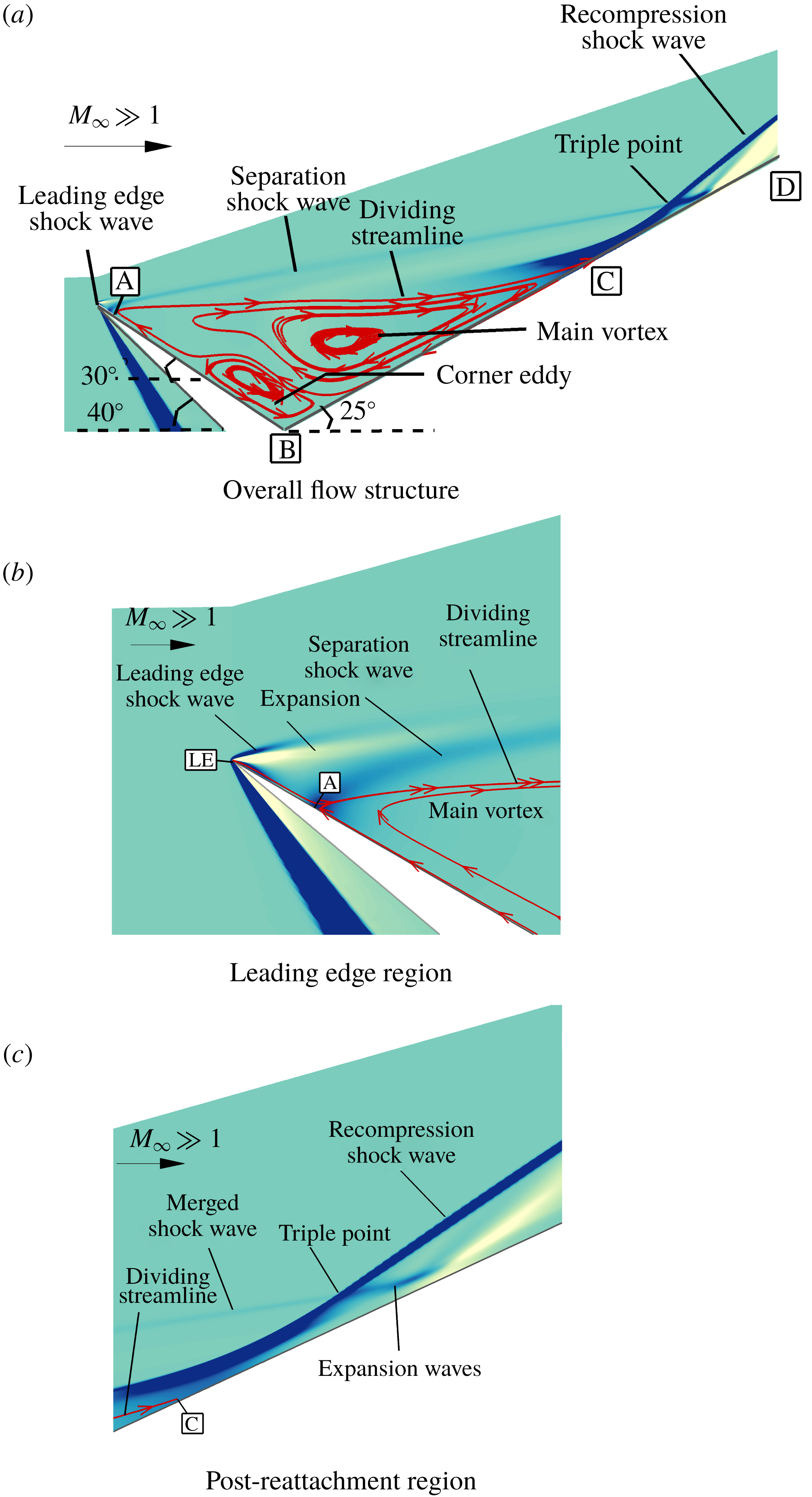
Geometry and flow structure of a hypersonic leading edge separation (a sharp leading edge).

2 Flow structure, geometry and free-stream conditions
A general schematic of leading edge separation under moderate enthalpy hypersonic conditions is shown in figure 1 with main flow features highlighted globally in figure 1(a), leading edge region in figure 1(b) and post-reattachment region in figure 1(c). Close to the leading edge
 $LE$
at
 $A$
(figure 1
b), the boundary layer separates and a shear layer emanates. If the compression surface
 $BD$
is sufficiently long, the shear layer reattaches at
 $C$
(figure 1
a). A recirculation region consequently forms, as seen in figure 1(a), and separates from the main inviscid outer flow by a dividing streamline, which is defined as the streamline leaving from the separation point
 $A$
and connecting at the reattachment point
 $C$
.
Under hypersonic conditions, a leading edge (bow) shock wave is formed due to viscous effects and the subsequent expansion is then followed by a separation shock which is analogous to a lip shock (Hama Reference Hama1968) as shown in figure 1(b). As the separation is very close to the leading edge in such a configuration, the leading edge and separation shocks merge into one and the resulting shock intersects the recompression shock at the triple point as shown in figure 1(c). The interaction between these two shocks of the same family results in an Edney Type VI interference with the expansion waves emanating from the triple point which then reflect from the surface as seen in figure 1(c).
In the present study, the leading edge separation configuration used is analogous to a compression corner geometry with a compression angle of
 $55^{\circ }$
but in which the forward surface has been rotated clockwise by
 $30^{\circ }$
. The length of the forward surface (expansion surface)
 $AB$
was chosen in all simulations as 20 mm so as to replicate the experimental model. The length of the recompression surface
 $BD$
, on the other hand, was varied from 50 mm in the sharp case to 80 mm in the blunt cases to accommodate for any increase in the size of separation due to bluntness.
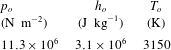
Flow conditions used in the present study were first obtained from previous work of Hruschka (Reference Hruschka2010) in a free-piston-driven shock tunnel, T-ADFA, at the University of New South Wales, Canberra. Tables 1 and 2 summarise these flow conditions, where
 $h,T,p,\unicode[STIX]{x1D70C}$
and
 $Re$
are specific enthalpy, temperature, pressure, density and Reynolds number, respectively, and subscripts ‘
 $o$
’ and ‘
 $\infty$
’ are nozzle reservoir and free-stream conditions, respectively.
Nozzle reservoir conditions (Hruschka Reference Hruschka2010).

Free-stream conditions (Hruschka Reference Hruschka2010).

3 Numerical procedure
3.1 Description of solver
Simulations in the present study were carried out using a continuum Navier–Stokes solver, US3D, which has been specifically developed at the University of Minnesota for high-speed flows (Nompelis & Candler Reference Nompelis and Candler2014; Candler et al. Reference Candler, Johnson, Nompelis, Gidzak, Subbareddy and Barnhardt2015). US3D is capable of performing perfect gas and real gas simulations and has also been validated over a wide range of geometries (Drayna, Nompelis & Candler Reference Drayna, Nompelis and Candler2006; Holden et al. Reference Holden, Wadhams, MacLean and Dufrene2013; Candler, Subbareddy & Brock Reference Candler, Subbareddy and Brock2014). The code uses parallel processing to improve the computational time and allows both implicit and explicit time integrations to be conducted.
The two-dimensional Cartesian representation of the discretised Navier–Stokes equations has been given in detail in Wright, Candler & Bose (Reference Wright, Candler and Bose1998), where flux terms are divided to inviscid and viscous components and Jacobian based on the sign of their eigenvalues. The code uses a cell-centred finite-volume formulation to numerically solve the Navier–Stokes equations. Steady-state solutions in the code are obtained using the modified Steger-Warming flux vector splitting method (Candler et al. Reference Candler, Johnson, Nompelis, Gidzak, Subbareddy and Barnhardt2015). The solver also uses Monotonic Upstream-Centred (MUSCL) Scheme (Van Leer Reference Van Leer1979) to achieve spatial accuracy of the second order. To prevent non-physical solutions from occurring, Osher limiter (Nompelis & Candler Reference Nompelis and Candler2014) has been utilised having good dissipation characteristics.
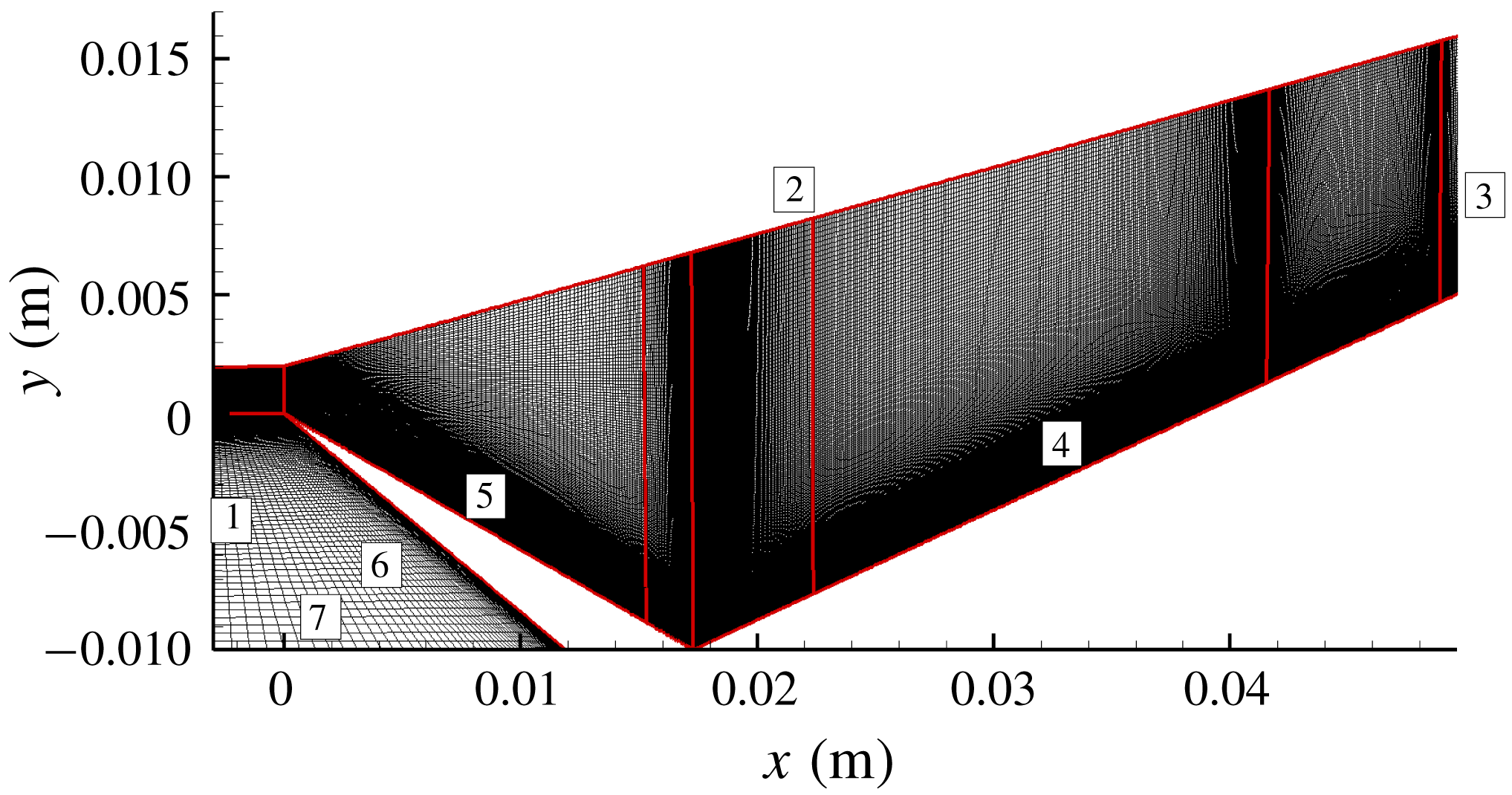
Coarse grid of the sharp leading edge case. The red lines define the blocks dividing the domain, while the labels refer to the boundary conditions.

Data-Parallel-Line-Relaxation method, used in US3D, has excellent convergence properties at a wide range of Reynolds numbers and well accommodates grid stretching common in hypersonic applications (Wright et al. Reference Wright, Candler and Bose1998). Implicit time integration scheme has further been selected to allow large Courant–Friedrichs–Lewy numbers to be used and obtain steady-state solutions.
It should be pointed out that simulations in the present study assume two-dimensional laminar flow and use perfect-gas air as the operating medium, which are adequate at the moderate enthalpy and Reynolds number flow in the present instance. Surfaces, on the other hand, are taken as non-catalytically isothermal with no velocity slip or temperature jump taking place. Real gas and slip effects on the present flow conditions and geometry are discussed in Khraibut (Reference Khraibut2018), where they were found to be minimum for both sharp and blunt leading edge configurations. These simulations, furthermore, show a maximum temperature of nearly 2300 K near reattachment, and bluntness to have no major effect on the peak temperature. Experimental measurements of translational temperature in the separated region were also taken by Le Page et al. (Reference Le Page, Barret, O’Byrne and Gai2019) using NO planar laser-induced fluorescence thermometry. They showed a maximum temperature of
 $2000\pm 500~\text{K}$
in the separated region. Their experiments only considered the
 $15~\unicode[STIX]{x03BC}\text{m}$
blunt leading edge. At such a temperature, it is not expected that real gas effects would be dominant.
3.2 Grid generation and boundary conditions
A commercial mesh generator, Pointwise, has been used to create grids used in the simulations. In the first case considered in the study (baseline case), in figure 2, the leading edge has been modelled as infinitesimally sharp. The main domain which encloses all edges 1 to 7 in the figure has been divided into blocks separated by the red lines to better control cell distribution in grid-sensitive areas such as the leading edge, corner and reattachment regions. Grid cells have also been clustered in such a way to allow resolution of flow features in these grid-sensitive regions. It should be noted that a fixed first cell height of
 $1~\unicode[STIX]{x03BC}\text{m}$
has been used in this and all subsequent refined grids 1 to 4. This first cell height has demonstrated sufficiency in resolving the boundary layer and intricate flow features and is also computationally economic. In figure 2, also, the boundary conditions were applied to edges numbered 1 to 7, where edges 1 and 2 are specified as velocity inlets, edges 3 and 7 as outflow and edges 4 to 6 as isothermal walls with a fixed temperature
 $T_{w}$
of 300 K.
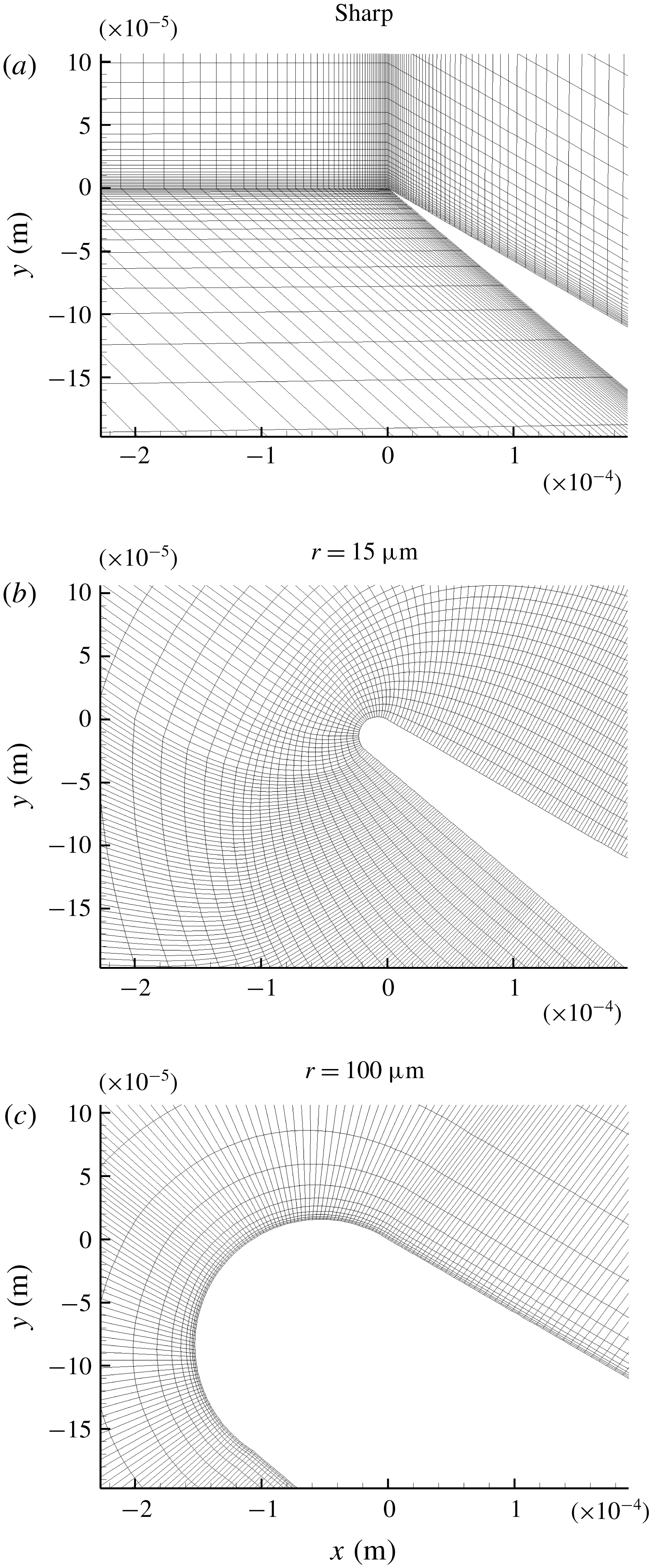
Magnified view of the leading edge region to show the clustering of cells in the sharp and blunt leading edge cases. Note: grids are coarsened in the
 $i$
and
 $j$
directions.

Bluntness was modelled by superposing a semicircular leading edge of radius
 $r=15~\unicode[STIX]{x03BC}\text{m}$
and
 $r=100~\unicode[STIX]{x03BC}\text{m}$
(figures 3(b) and 3(c), respectively) on the origin of the sharp leading edge case (figure 3
a). Grid points were distributed evenly along the circumference in both blunt leading edge cases, and numbers of points were subsequently increased with grid refinement (see tables 4 and 5). To account for the increase in size of separation due to bluntness, the length of the compression surface (edge 4 in figure 2) was extended to 80 mm from 50 mm used in the sharp leading edge case. To ensure cell orthogonality on the wall, the normal extrusion function in Pointwise was used in the blunt leading edge cases. The boundary conditions in these case were specified as in the sharp leading edge case (see figure 2).
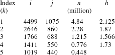
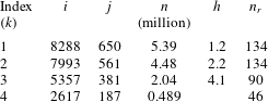
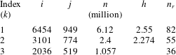
Tables 3 to 5 summarise the grids used in the simulations with
 $k$
indicating grid index, number of nodes in the
 $x$
and
 $y$
directions represented with index
 $i$
and index
 $j$
, respectively, total number of cells is
 $n$
, compression ratio is defined as
 $h=n_{k+1}/n_{k}$
and finally number of cells on leading edge radius is
 $n_{r}$
.
Summary of grids used in the sharp leading edge simulations.
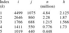
Summary of grids used in the small bluntness leading edge (
 $r=15~\unicode[STIX]{x03BC}\text{m}$
) simulations.

Summary of grids used in the large bluntness leading edge (
 $r=100~\unicode[STIX]{x03BC}\text{m}$
) simulations.

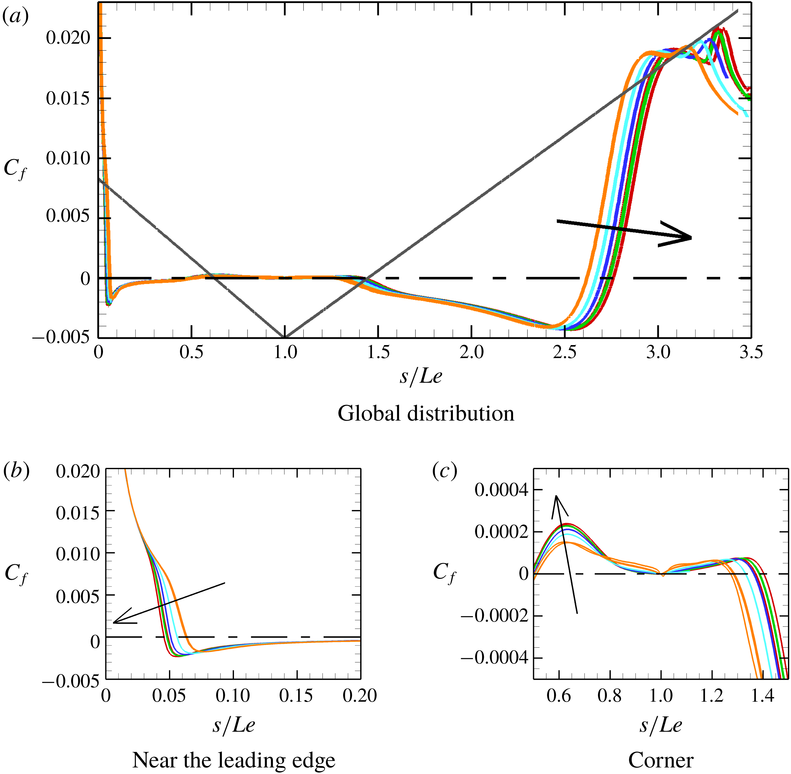
Convergence trend of the shear stress
 $C_{f}$
over the surface. Grid 1 (red): 3- to 6-order drop in RMS residuals; grid 2 (green): 2- to 6-order drop in RMS residuals; grid 3 (blue): 3- to 7-order drop in RMS residuals; grid 4 (turquoise): 3- to 7-order drop in RMS residuals; grid 5 (orange): 3- to 7-order drop in RMS residuals. Arrows indicate the direction of iterative and grid convergence. The different lines of the same colour correspond to the different convergence levels. Note that some convergence levels are indistinguishable. Grey line: surface; dashed-dotted line:
 $C_{f}=0$
.

3.3 Grid convergence details
3.3.1 Sharp leading edge simulations
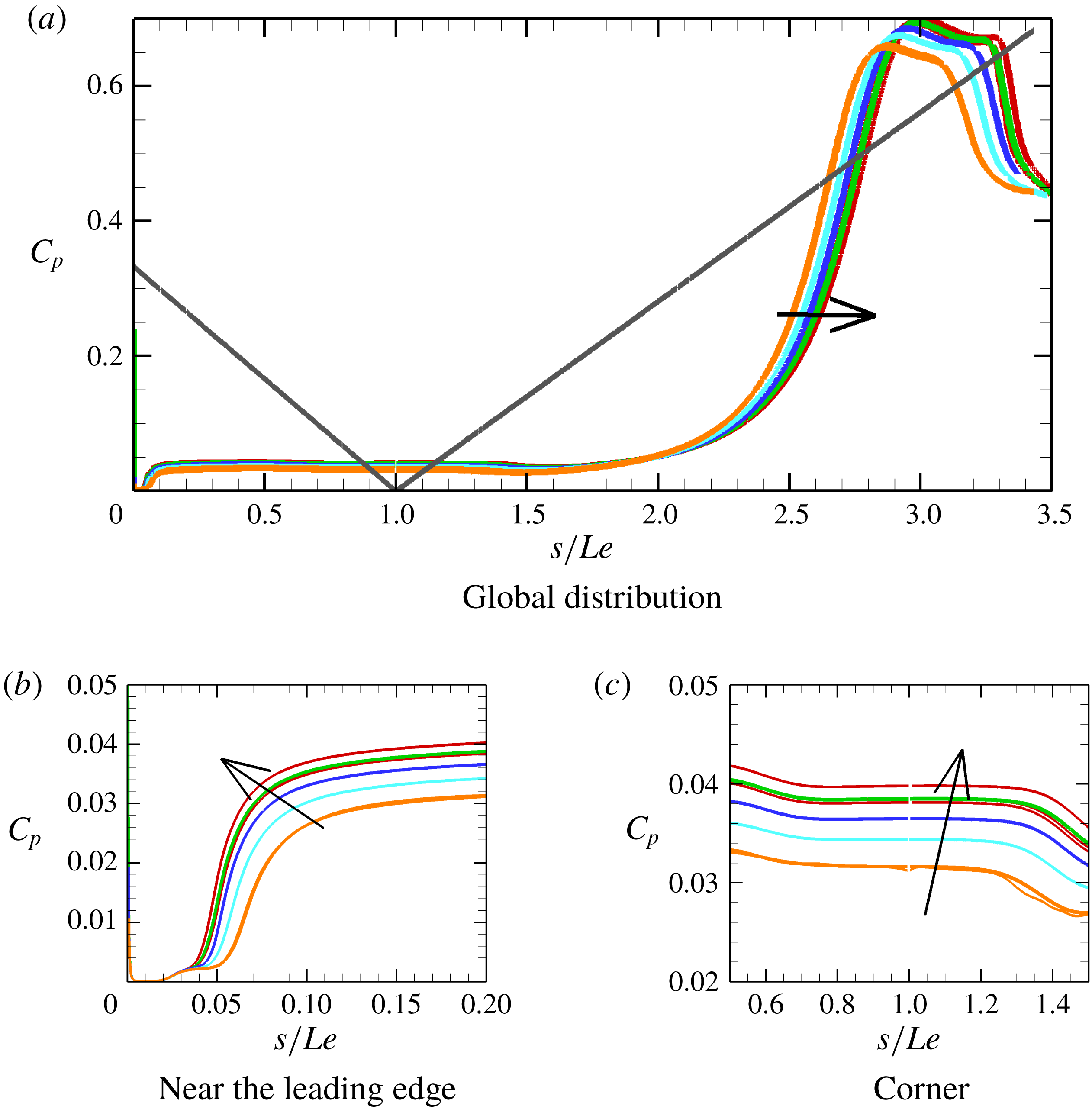
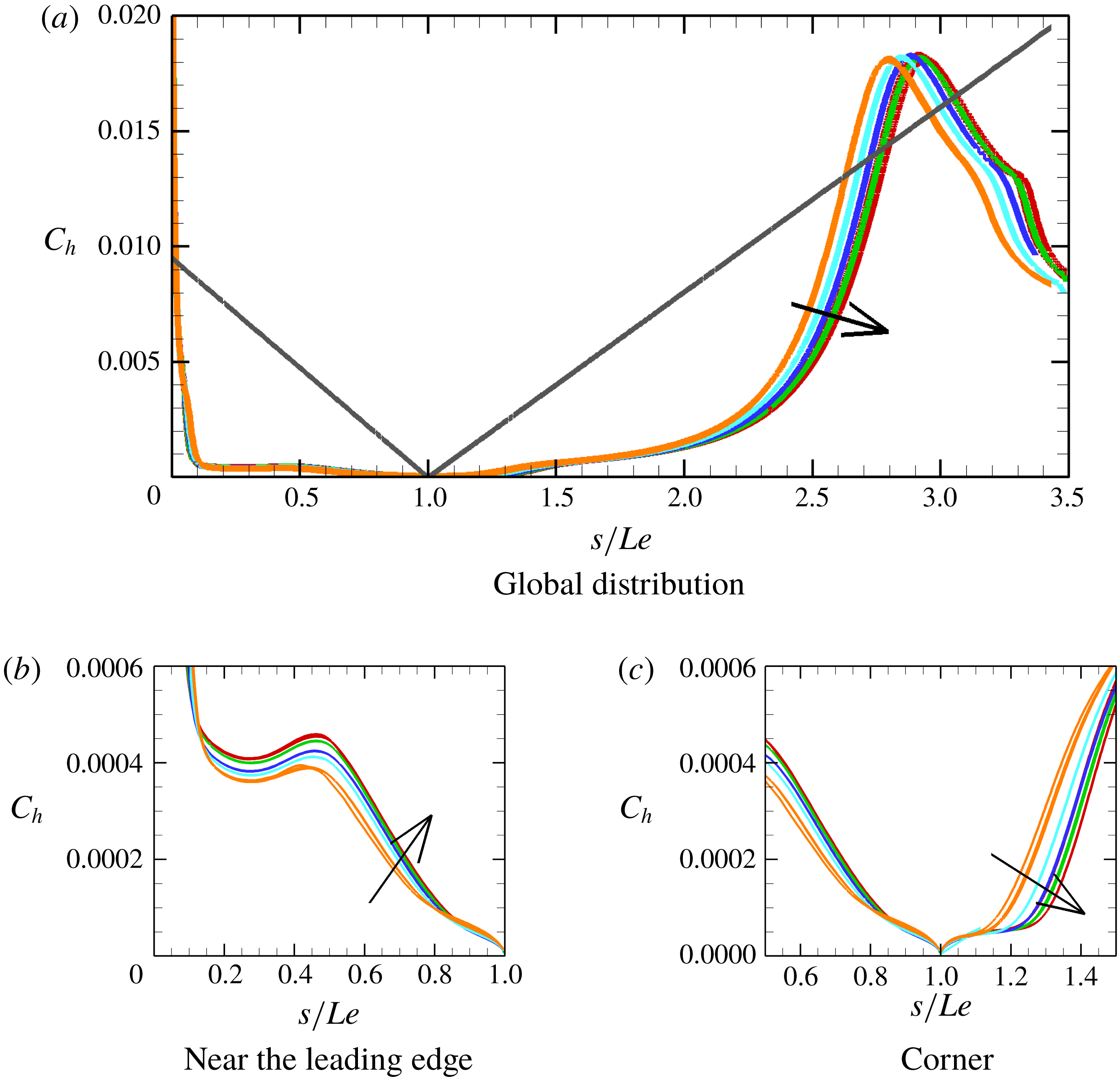
Surface distributions of parameters such as the shear stress, pressure and heat flux are typically monitored for convergence in separated flows. Here, convergence means both iterative and grid convergence. Whereas the latter is concerned with grid refinement, the former indicates whether a steady state has been reached in each grid. Iterative convergence is usually monitored by the root mean square (RMS) residuals, which are given here by the solver. The term ‘convergence level’ is used throughout the paper to refer to the order drop in RMS residuals. During the grid convergence study, it was noted that attainment of a steady state requires, at least, five-order drop in RMS residuals, if the solution was initialised from free-stream conditions, and less if it was initialised from a previously converged solution. Figures 4–6 show surface parameters (shear stress, pressure and heat flux) for grids used in the sharp case with each distinguishable line in the same grid referring to a different convergence level.
Convergence trend of the pressure
 $C_{p}$
over the surface. Grid 1 (red): 3- to 6-order drop in RMS residuals; grid 2 (green): 2- to 6-order drop in RMS residuals; grid 3 (blue): 3- to 7-order drop in RMS residuals; grid 4 (turquoise): 3- to 7-order drop in RMS residuals; grid 5 (orange): 3- to 7-order drop in RMS residuals. Arrows indicate the direction of iterative and grid convergence. The different lines of the same colour correspond to the different levels. Note that some convergence levels are indistinguishable. Grey line: surface.

The shear stress, though particularly important in defining the size of separation, is generally difficult to measure in short-duration facilities. More often, it is surface pressure and heat flux that are measured and reported in experimental studies. In this study, being mainly numerical, all surface parameters (shear stress, pressure and heat flux) are shown non-dimensionalised, for the sharp leading edge case, in figures 4–6 against the wetted distance
 $s/Le$
. In these figures,
 $C_{f}$
is the skin friction coefficient,
 $C_{p}$
is a surface pressure coefficient defined as the ratio of
 $p$
and dynamic pressure
 $0.5\unicode[STIX]{x1D70C}_{\infty }U_{\infty }^{2}$
and
 $C_{h}$
is a heat flux coefficient defined as the ratio of heat flux
 $q_{w}$
and quantity
 $0.5\unicode[STIX]{x1D70C}_{\infty }U_{\infty }^{3}$
.
Considering the shear stress data (figure 4) first, the size of the separation region can be determined from the shear stress as it crosses the zero line (dashed-dotted line) from positive to negative at separation, and from negative to positive at reattachment. In the corner region (figure 4 c), we further note that multiple crossings of the zero line are present so that a smaller secondary vortex embeds within the main vortex. Earlier studies by Khraibut et al. (Reference Khraibut, Deepak, Gai and Neely2014) and Khraibut, Gai & Neely (Reference Khraibut, Gai and Neely2015) showed secondary vortices are particularly sensitive to grid resolution and solution progression with number of iterations. In this study, therefore, they are monitored along with the main vortex for convergence.
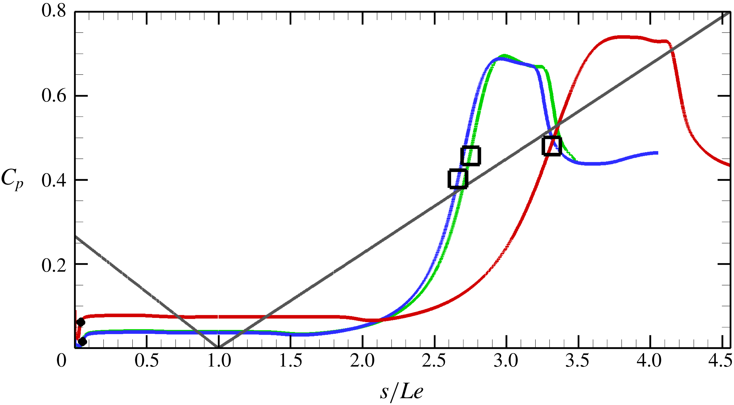
Global surface pressure distribution is shown in figure 5(a) with close-up views of the leading edge region and the corner in figures 5(b) and 5(c), respectively. Figure 5(b) shows the boundary layer growth prior to separation, which seems to decrease in length with grid refinement. Global pressure distribution in figure 5(a) shows a downstream movement of pressure peaks after reattachment which become sharper with refinement. The pressure peaks and subsequent dips are the result of Edney Type VI interference as mentioned earlier in § 2. As the separation size increases with grid refinement, we note that the pressure plateau in the corner region also increases (figure 5 c).
Heat flux distribution over the surface is similarly shown in figure 6, where variations due to grid refinement are seen in the leading edge, corner and reattachment regions.
Convergence trend of the heat flux
 $C_{h}$
over the surface. Grid 1 (red): 3- to 6-order drop in RMS residuals; Grid 2 (green): 2- to 6-order drop in RMS residuals; grid 3 (blue): 3- to 7-order drop in RMS residuals; grid 4 (turquoise): 3- to 7-order drop in RMS residuals; grid 5 (orange): 3- to 7-order drop in RMS residuals. Arrows indicate the direction of iterative and grid convergence. The different lines of the same colour correspond to the different convergence levels. Note that some convergence levels are indistinguishable. Grey line: surface.

3.3.2 Blunt leading edge simulations
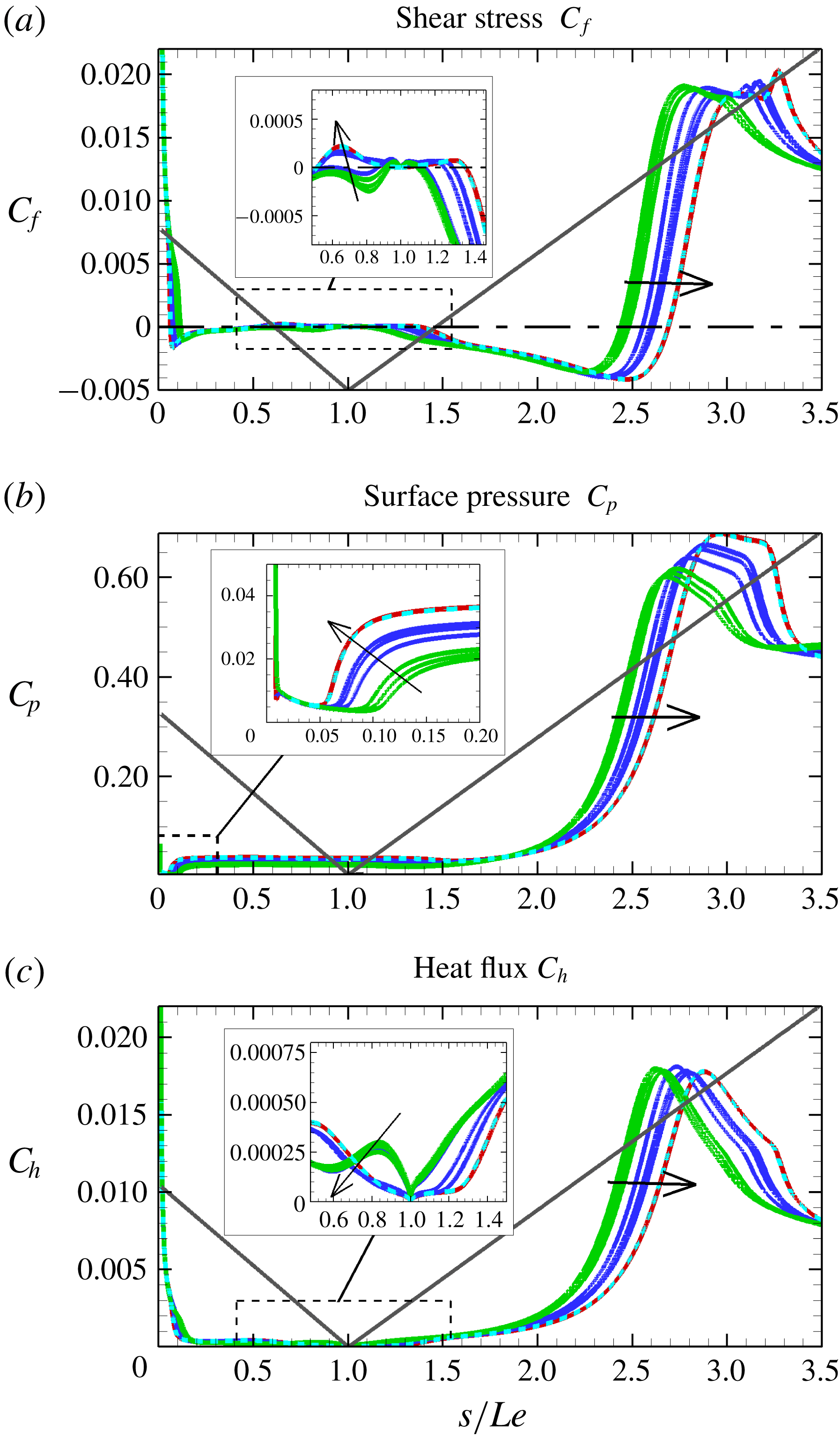
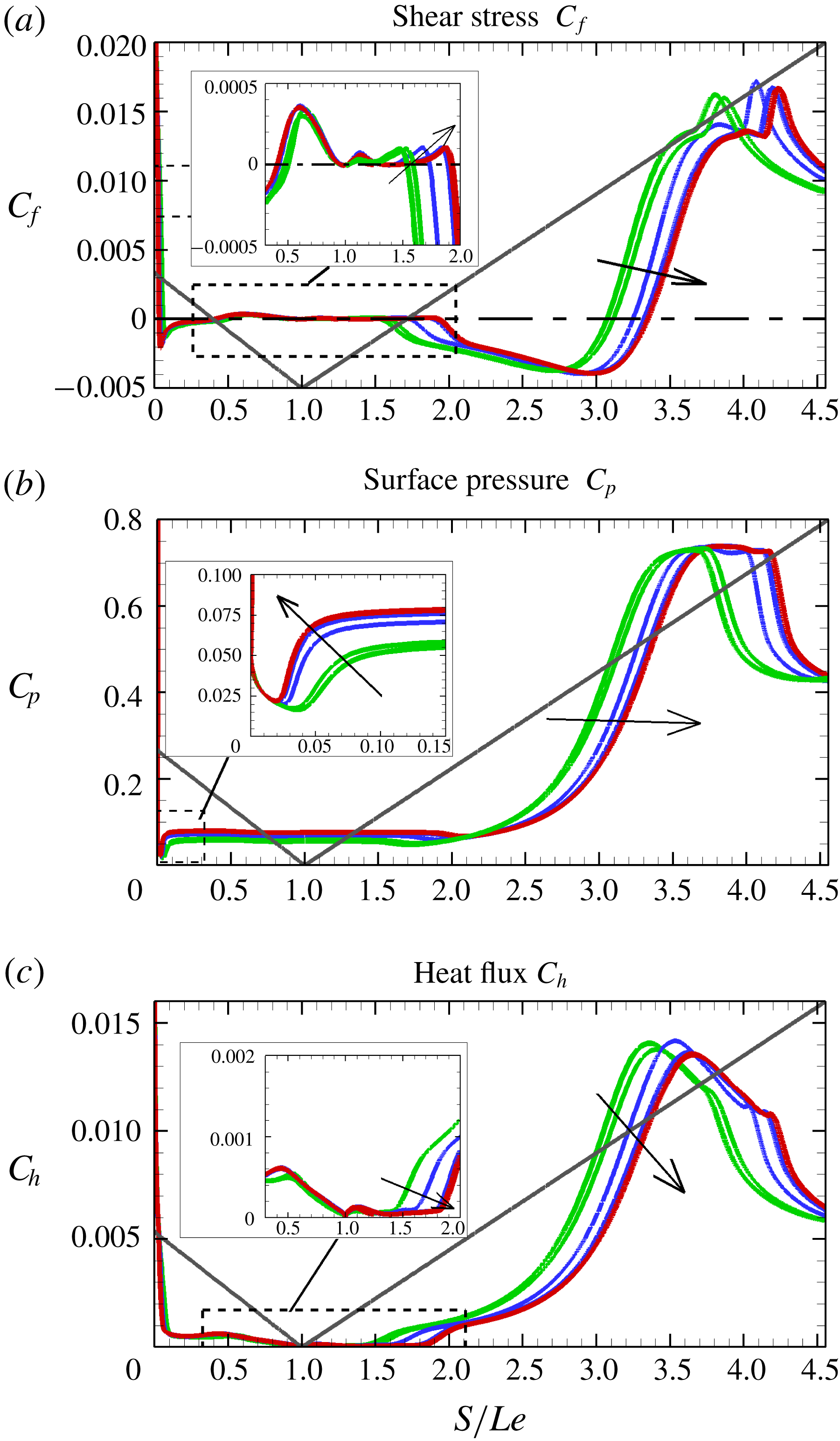
Convergence trends of blunt leading edge simulations are shown for
 $r=15~\unicode[STIX]{x03BC}\text{m}$
in figure 7 and in figure 8 for
 $r=100~\unicode[STIX]{x03BC}\text{m}$
. For the small bluntness
 $r=15~\unicode[STIX]{x03BC}\text{m}$
simulations, the shear stress shows grid 4 to be too coarse to fully capture flow features, mainly the secondary vortex within the main separation, while grid 1 and grid 2 show no appreciable differences in the predictions of surface pressure, shear stress and heat flux. Grid 2 is therefore taken as the minimum requirement for grid convergence.
Large bluntness
 $r=100~\unicode[STIX]{x03BC}\text{m}$
simulations, on the other hand, all show, through the shear stress distributions, that a tertiary eddy/vortex exists in all grids used in the simulations. Grid 3, however, is found to underpredict the separation compared to grids 1 and 2. Grids 1 and 2, on the other hand, are in good agreement in their predictions of surface parameters. Here too, grid 2 is taken as the minimum required for grid convergence.
Convergence data of the small bluntness (
 $r=15~\unicode[STIX]{x03BC}\text{m}$
) case. Grid 1 (turquoise): 3- to 5-order drop in RMS residuals; grid 2 (red): 5- to 6-order drop in RMS residuals; grid 3 (blue): 5- to 7-order drop in RMS residuals; grid 4 (green): 4- to 7-order drop in RMS residuals. Arrows indicate the direction of iterative and grid convergence. The different lines of the same colour correspond to the different convergence levels. Note that some convergence levels are indistinguishable. Grey line: surface; dash-dotted line:
 $C_{f}=0$
.

Convergence data of the large bluntness (
 $r=100~\unicode[STIX]{x03BC}\text{m}$
) case. Red: grid 1; blue: grid 2; green: grid 3. Grids are shown for convergence levels corresponding to 4- to 7-order drop in RMS residuals with the arrows pointing in the direction of convergence. The different lines of the same colour correspond to the different convergence levels. Note that some convergence levels might be indistinguishable. Grey lines: surface; dash-dotted line:
 $C_{f}=0$
. Dashed boxes are regions shown in insets.

Spatial errors (%) at separation (subscript ‘
 $S$
’) and reattachment (subscript ‘
 $R$
’) of the main (subscript ‘1’) and secondary (subscript ‘2’) vortices in the sharp bluntness (
 $r=15~\unicode[STIX]{x03BC}\text{m}$
) leading edge simulations;
 $s/Le$
is the wetted distance normalised by the length of the expansion surface.

Spatial errors (%) at separation (subscript ‘
 $S$
’) and reattachment (subscript ‘
 $R$
’) of the main (subscript ‘1’) and secondary (subscript ‘2’) vortices in the small bluntness (
 $r=15~\unicode[STIX]{x03BC}\text{m}$
) leading edge simulations;
 $s/Le$
is the wetted distance normalised by the length of the expansion surface.

Spatial errors (%) at separation (subscript ‘
 $S$
’) and reattachment (subscript ‘
 $R$
’) of the main (subscript ‘1’) and secondary (subscript ‘2’) vortices in the large bluntness (
 $r=100~\unicode[STIX]{x03BC}\text{m}$
) leading edge simulations;
 $s/Le$
is the wetted distance normalised by the length of the expansion surface.

3.4 Grid error analysis
The mixed-order method is used to carry out a systematic grid error analysis as it deals well with flow discontinuities such as shock waves. The method has been described in detail by Roy (Reference Roy2003), where both first-order and second-order terms are retained in the generalised Richardson extrapolation technique,
 $$\begin{eqnarray}\displaystyle f=f_{exact}+g_{1}h+g_{2}h^{2}+O(h^{3}), & & \displaystyle\end{eqnarray}$$
which requires all grid solutions to be within the asymptotic range of
 $f_{exact}$
and continuous. Expanding (3.1) to at least three grids yields an exact solution as
 $$\begin{eqnarray}f_{exact}=f_{1}+\frac{\unicode[STIX]{x1D716}_{32}(r_{12}-1)-\unicode[STIX]{x1D716}_{21}(r_{12}r_{23}^{2}-r_{12}-r_{23}-1)}{(r_{12}-1)(r_{23}-1)(r_{12}r_{23}-1)},\end{eqnarray}$$
where
 $\unicode[STIX]{x1D716}_{32}=f_{3}-f_{2}$
,
 $\unicode[STIX]{x1D716}_{21}=f_{2}-f_{1}$
,
 $r_{12}=h_{1}/h_{2}$
and
 $r_{23}=h_{2}/h_{3}$
.
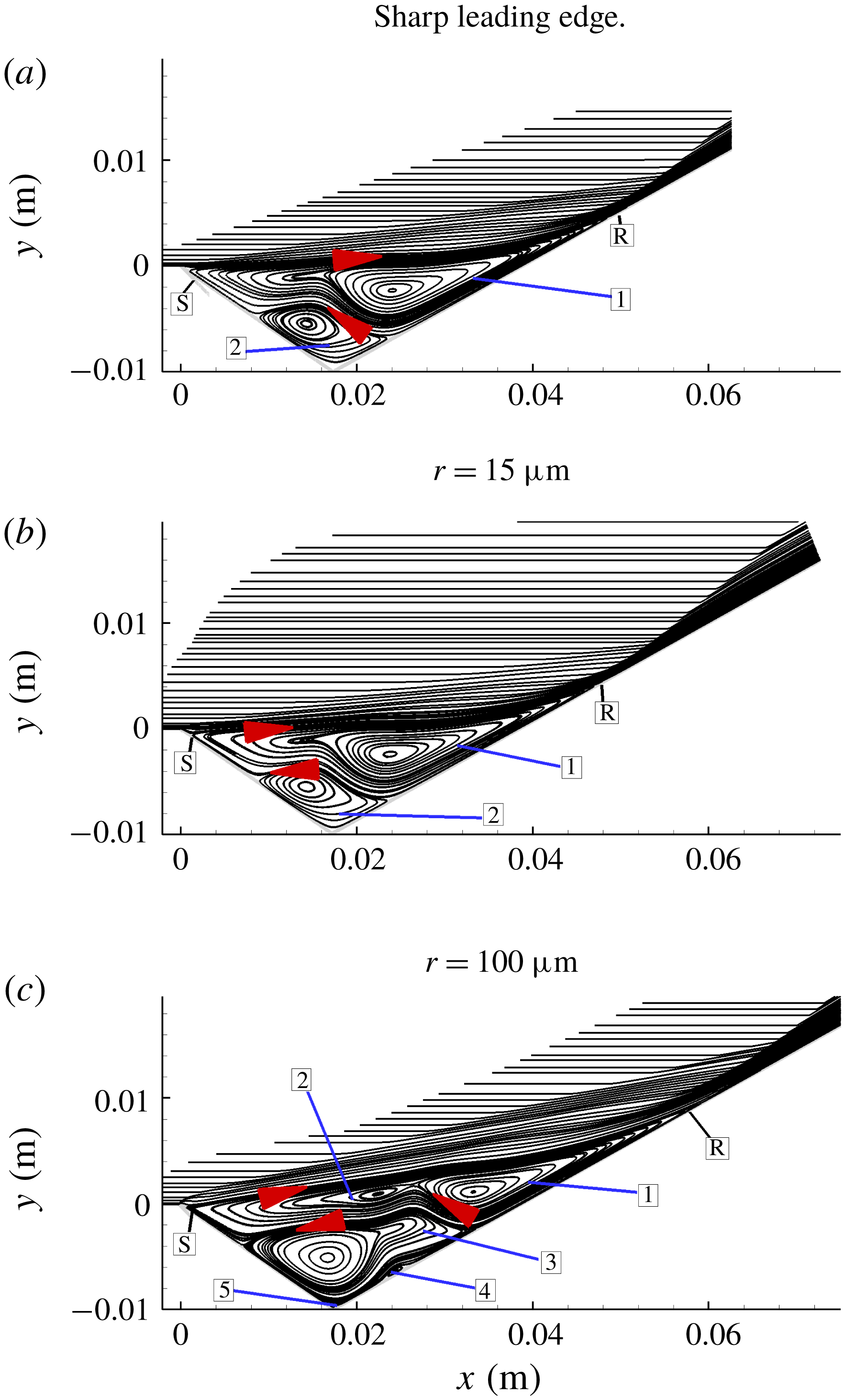
Overall streamlines in the sharp and blunt leading edge simulations, where the arrows point in the direction of recirculation and the numbers refer to the vortices.

The term
 $f_{exact}$
can be evaluated for any parameter of interest to convergence, which in the case of separated flows are surface parameter at separation
 $S$
and reattachment
 $R$
. In the case where multiple vortices are present, however, they too become important in dictating convergence. The spatial error is calculated as
 $$\begin{eqnarray}|\mathit{Spatial~error}|=3\left|\frac{f_{1-3}-f_{exact}}{f_{exact}}\right|\times 100,\end{eqnarray}$$
and hence evaluated at the main and secondary separations (subscripts ‘1’ and ‘2’, respectively), but with the expansion length
 $L_{e}$
used in the denominator of (3.3) to avoid division by zero in the calculation of the main separation. The constant ‘3’ seen in the equation is a safety factor to give a conservative estimate of the error.
Effects of grid refinement on spatial errors of all of
 $S_{1}$
,
 $R_{1}$
,
 $S_{2}$
and
 $R_{2}$
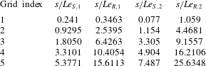
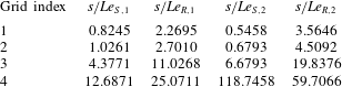
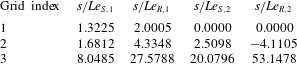
are summarised in tables 6–8 for the sharpest to the largest bluntness cases. These tables show that
 $S_{1}$
and
 $S_{2}$
move upstream towards the leading edge with grid refinement indicating an earlier separation, while the opposite trend is seen in the movement of
 $R_{1}$
and
 $R_{2}$
, which demonstrates a downstream movement with refinement. More importantly, the spatial errors show a slower convergence for secondary vortices and grid 2 can be taken as a grid converged with confidence with errors less than 5 %. The results presented in the discussion section are, therefore, based on grid 2 for all cases.
4 Results and discussion
4.1 Effect of bluntness on flow structure
The first part of the discussion will investigate the effect of leading edge bluntness on the main and secondary vortices. In figure 9, these features are shown for an idealised sharp leading edge case, a finite small bluntness case with
 $r=15~\unicode[STIX]{x03BC}\text{m}$
and a large bluntness case of
 $r=100~\unicode[STIX]{x03BC}\text{m}$
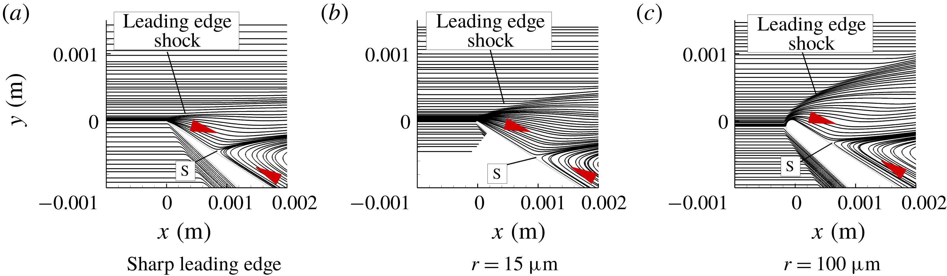
. As separation in all cases occurs very close to the leading edge, a magnified view of the flow near the leading edge is presented in figure 10. Separation and reattachment are denoted by ‘S’ and ‘R’, respectively, while the vortices are numbered.
Magnified view of the streamlines near the leading edge. Arrows point in the direction of recirculation.

Considering figure 9 first, it can be seen that with the small bluntness, overall, there is little difference in terms of the size of separation, streamlines, shock wave structure and strength, and number of vortices, compared to the ideally sharp case. It appears that the main effect of introducing small bluntness to the leading edge is to create a bow shock wave, which results in local reduction of the Reynolds number, and causes the separation to occur slightly downstream, compared to the sharp leading edge case (see also figure 18 g,h). Second, as the interaction process is not free, in the Chapman sense, the reattachment is also affected by the small bluntness and moves slightly upstream so that the separated region is smaller than that of the sharp leading edge case.
A reverse effect, however, is seen by increasing bluntness from
 $15$
to
 $100~\unicode[STIX]{x03BC}\text{m}$
(see also figure 18
h,i) so that in the larger bluntness case the separated region increases in size by the upstream movement of ‘S’ and downstream movement of ‘R’. With increased bluntness, also, a total of five vortices appear within the separated region, where vortex 1 and vortex 2 form the primary separation, vortex 3 is a larger corner vortex and 4 and 5 are smaller eddies residing on compression surface and vertex, respectively.
From figures 9(c) and 10(c), a stronger bow shock can be seen in the large bluntness case and consequently the shock–shock interaction (Edney Type VI) is strengthened. It is emphasised that the above analysis ignores viscous effects as well as effects of multiple vortices in the main separation region and a non-isentropic recompression.
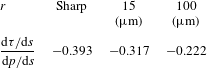
Figure 10 also shows that the location of stagnation point in the case of figure 10(c) moves slightly below on the windward surface. This is because bluntness was incorporated by superposing a radius on the baseline sharp geometry. Bluntness shows that angle and shape of the dividing streamline at ‘S’ are different for sharp/small bluntness compared to large bluntness leading edge. In the large bluntness case, the streamline leaves the surface with a smaller separation angle, while sharp/small bluntness leading edge leaves at a larger angle. The inclination of separation streamline to the surface can be described as (Oswatitsch Reference Oswatitsch1957)
 $$\begin{eqnarray}\displaystyle \unicode[STIX]{x1D703}_{s}=\tan ^{-1}\left(-3\frac{\text{d}\unicode[STIX]{x1D70F}/\text{d}s}{\text{d}p/\text{d}s}\right), & & \displaystyle\end{eqnarray}$$
where
 $\unicode[STIX]{x1D703}_{s}$
is the streamline angle at separation and
 $\text{d}\unicode[STIX]{x1D70F}/\text{d}s$
and
 $\text{d}p/\text{d}s$
are the streamwise shear stress and pressure gradients at separation, respectively. The Oswatisch relation more importantly implies that at a large separation angle (
 $\unicode[STIX]{x1D703}_{s}>45^{\circ }$
)
 $$\begin{eqnarray}-\frac{\text{d}\unicode[STIX]{x1D70F}}{\text{d}s}>\frac{1}{3}\frac{\text{d}p}{\text{d}s}.\end{eqnarray}$$
This means that a higher
 $\unicode[STIX]{x1D703}_{s}$
is caused by a decrease in
 $\text{d}\unicode[STIX]{x1D70F}/\text{d}s$
and an increase in
 $\text{d}p/\text{d}s$
. Table 9 shows the ratio of
 $\text{d}\unicode[STIX]{x1D70F}/\text{d}s$
to
 $\text{d}p/\text{d}s$
for all cases. We note that compared to the sharp case, for the small bluntness case (
 $r=15~\unicode[STIX]{x03BC}\text{m}$
) this ratio is reduced by 21.5 %, whereas for the larger bluntness case (
 $r=100~\unicode[STIX]{x03BC}\text{m}$
) it is reduced by nearly 55.7 %. In terms of the separation angle
 $\unicode[STIX]{x1D703}_{s}$
, this is a reduction to
 $43^{\circ }$
and
 $33.66^{\circ }$
compared to the sharp leading edge separation angle of
 $49.75^{\circ }$
. These results are consistent with figure 10 showing a reduction in inclination of the streamline at ‘S’ from the surface with increased bluntness.
Closer examination of figure 10 shows curvature of the separation streamline as it emerges from the surface. Here we note that it is convex to the oncoming flow in the case of figure 10(a,b) and slightly concave in figure 10(c). These observations are consistent with those by Smith (Reference Smith1986), who noted, based on the triple-deck theory, the separation streamline to be concave in subsonic flows, straight in supersonic flows and convex in hypersonic flows in that increase in leading edge bluntness also increases strength of the bow shock wave. A largely subsonic region is created behind the shock wave which thereby ameliorates the curvature of the separation streamline.
Ratio of the shear stress and pressure gradients
 $\text{d}\unicode[STIX]{x1D70F}/\text{d}s$
and
 $\text{d}p/\text{d}s$
, respectively, at separation for the sharp and blunt leading edge cases.

4.2 Surface parameters
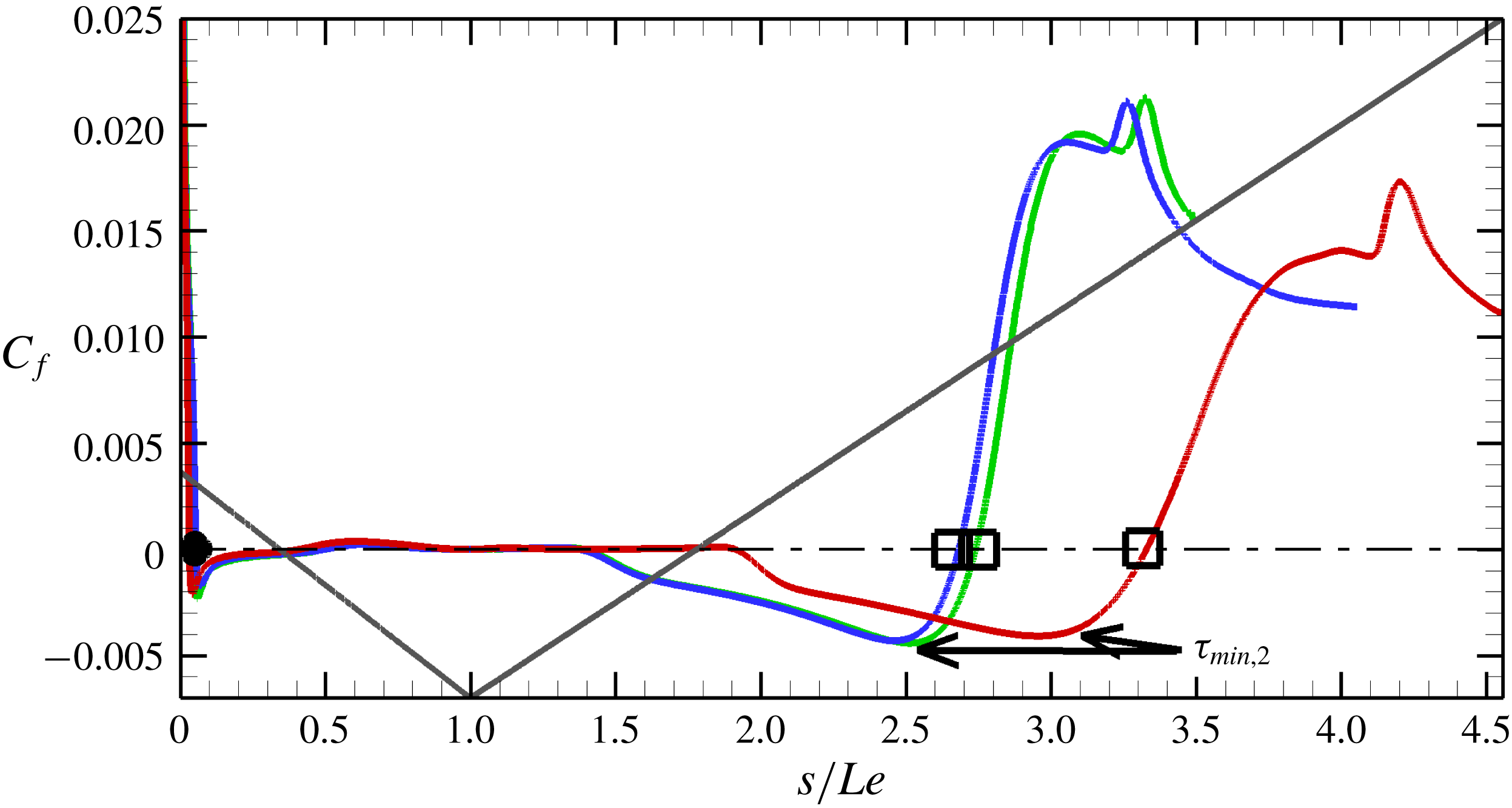
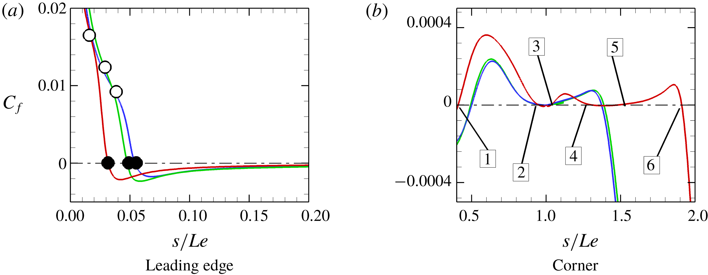
Surface data (shear stress, pressure and heat flux) are shown on a global scale in figures 11, 13 and 15. The shear stress in figure 11 shows a large increase in size of separation for the large bluntness of
 $r=100~\unicode[STIX]{x03BC}\text{m}$
. This is manifested in the upstream movement of ‘S’ accompanied by downstream movement of ‘R’. The small bluntness (
 $r=15~\unicode[STIX]{x03BC}\text{m}$
) leading edge, on the other hand, shows a small reduction due to the introduction of bluntness to the geometry, compared to the ideal sharp case (figure 12
a). The vicinity of the corner in figure 12(b) further shows a multiple vortex structure for the large bluntness case, which is inferred by shear stress lines crossing the zero line six times. The corner shear stresses for the sharp/small bluntness cases, on the other hand, show primary and secondary separations. This indicates the fragmentation within the recirculation region is promoted by bluntness.
Bluntness effects on the shear stress
 $C_{f}$
. Green line: sharp leading edge; blue line: small blunt leading edge (
 $r=15~\unicode[STIX]{x03BC}\text{m}$
); red line: large blunt leading edge (
 $r=100~\unicode[STIX]{x03BC}\text{m}$
); grey line: surface. Filled circles: separation; open squares: reattachment.

Bluntness effects on the shear stress
 $C_{f}$
near the leading edge and corner. Green line: sharp leading edge; blue line: small blunt leading edge (
 $r=15~\unicode[STIX]{x03BC}\text{m}$
); red line: large blunt leading edge (
 $r=100~\unicode[STIX]{x03BC}\text{m}$
). Filled circles: separation; open circles: beginning of interaction.

An additional important observation from figure 11 is the change occurring in the second shear stress minimum (seen immediately before reattachment) with bluntness. We note that as bluntness becomes large, there is a small reduction in the magnitude of this minimum and it also becomes shallower compared to the sharp and small bluntness cases. Such a second minimum in the shear stress is characteristic of large closed separations. This feature has been discussed by Smith (Reference Smith1988). Smith put forward the possibility of this second minimum in shear stress approaching singularity (
 $\unicode[STIX]{x1D70F}_{min,2}\rightarrow -\infty$
) if the parameter
 $\unicode[STIX]{x1D703}$
governing the interaction reaches a critical value. Smith termed this condition ‘reversed flow singularity’, which is an asymptotic limit and assumes very high Reynolds number flow. Angle
 $\unicode[STIX]{x1D703}$
, the scaled triple-deck angle, is defined in Stewartson (Reference Stewartson1970) as
 $$\begin{eqnarray}\displaystyle \unicode[STIX]{x1D703}=\frac{\unicode[STIX]{x1D703}^{\ast }Re^{1/4}}{C^{1/4}\unicode[STIX]{x1D706}^{1/2}(M^{2}-1)^{1/2}}, & & \displaystyle\end{eqnarray}$$
where
 $\unicode[STIX]{x1D703}^{\ast }$
is the agent causing the separation (for example, a compression corner angle),
 $Re$
is a characteristic Reynolds number,
 $C$
is the Chapman–Rubesin parameter,
 $\unicode[STIX]{x1D706}$
is the shear constant and in hypersonic flows where
 $M\gg 1$
the quantity
 $(M^{2}-1)^{1/2}\rightarrow M$
.
It is interesting to point out the similarity between the results of figure 11 and earlier results of wall temperature effects on leading edge separation (Khraibut et al. Reference Khraibut, Gai, Brown and Neely2017; Khraibut Reference Khraibut2018), which also showed that the second shear stress minimum becomes shallower but increases in magnitude with increasing wall temperature. It is possible that both effects (bluntness and wall temperature) result in an overall reduction of local Reynolds number relieving gradients near the second minimum.
Bluntness effects on the surface pressure
 $C_{p}$
distribution. Green line: sharp leading edge; blue line: small blunt leading edge (
 $r=15~\unicode[STIX]{x03BC}\text{m}$
); red line: large blunt leading edge (
 $r=100~\unicode[STIX]{x03BC}\text{m}$
); grey line: surface. Filled circles: separation; open squares: reattachment.

Bluntness effects on the surface pressure
 $C_{p}$
distribution near corner. Green line: sharp leading edge; blue line: small blunt leading edge (
 $r=15~\unicode[STIX]{x03BC}\text{m}$
); red line: large blunt leading edge (
 $r=100~\unicode[STIX]{x03BC}\text{m}$
). Filled circles: separation; open circles: beginning of interaction.

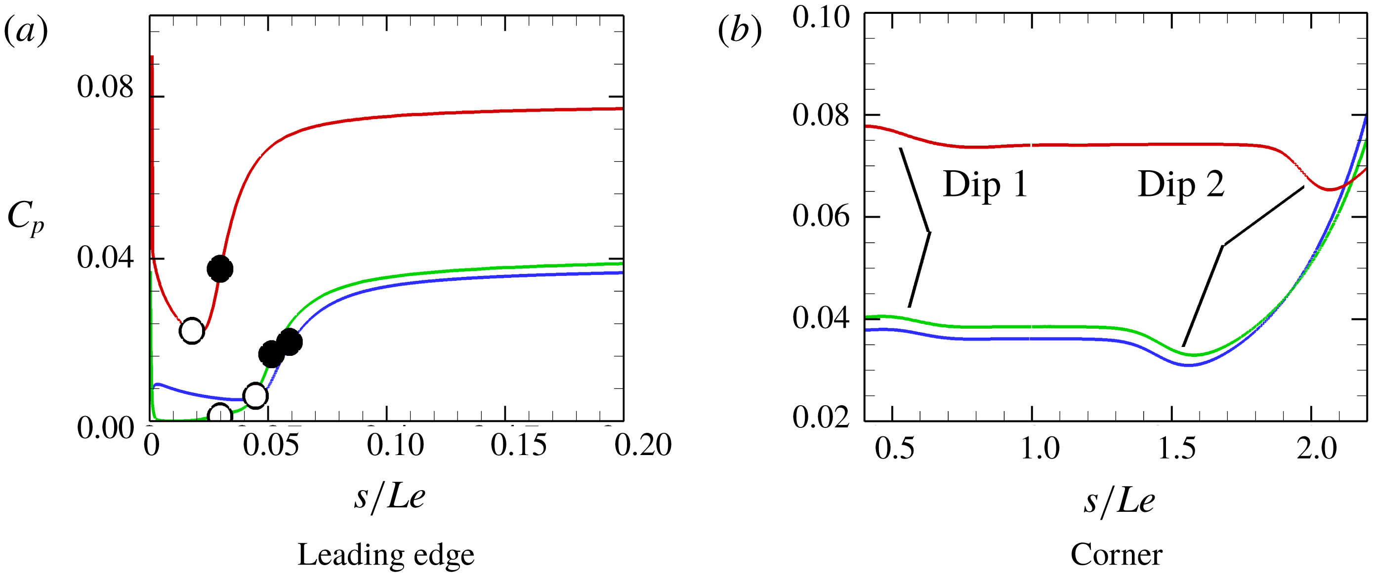
Bluntness effect on surface pressures is shown in figure 13. Details near the leading edge and in the vicinity of corner are shown in figure 14(a,b). Delay in separation due to the introduction of small bluntness (
 $r=15~\unicode[STIX]{x03BC}\text{m}$
) from the sharp case can be clearly seen. A slightly favourable pressure gradient is noted with the small bluntness leading edge just before separation (drop in
 $C_{p}$
before interaction). In the large bluntness case (
 $r=100~\unicode[STIX]{x03BC}\text{m}$
) in figure 14(a), on the other hand, separation occurs closer to the leading edge as the boundary layer starts to develop (see locations of open and filled circles in figure 14
a).
In figure 14(b), the corner region shows two dips near
 $s/Le\approx 0.5$
and
 $s/Le\approx 1.5$
in the sharp/small bluntness cases and
 $s/Le\approx 0.5$
and
 $s/Le\approx 2$
in the large bluntness case. The locations of these dips occur just before the secondary vortex separates (dip 2) then reattaches (dip 1). These dips more importantly show that both streamwise and normal pressure gradients exist in the flow, which provides a mechanism by which multiple vortices could develop, within a separated region, as the RBL begins to separate. We also see in figure 13 that the pressure overshoot after reattachment increases as a result of increasing bluntness. This increases the bow shock wave’s strength in front of the leading edge, which leads to an increase in the global and plateau pressures (figure 14
a,b). Effect of bluntness on the RBL will be discussed in § 4.4.
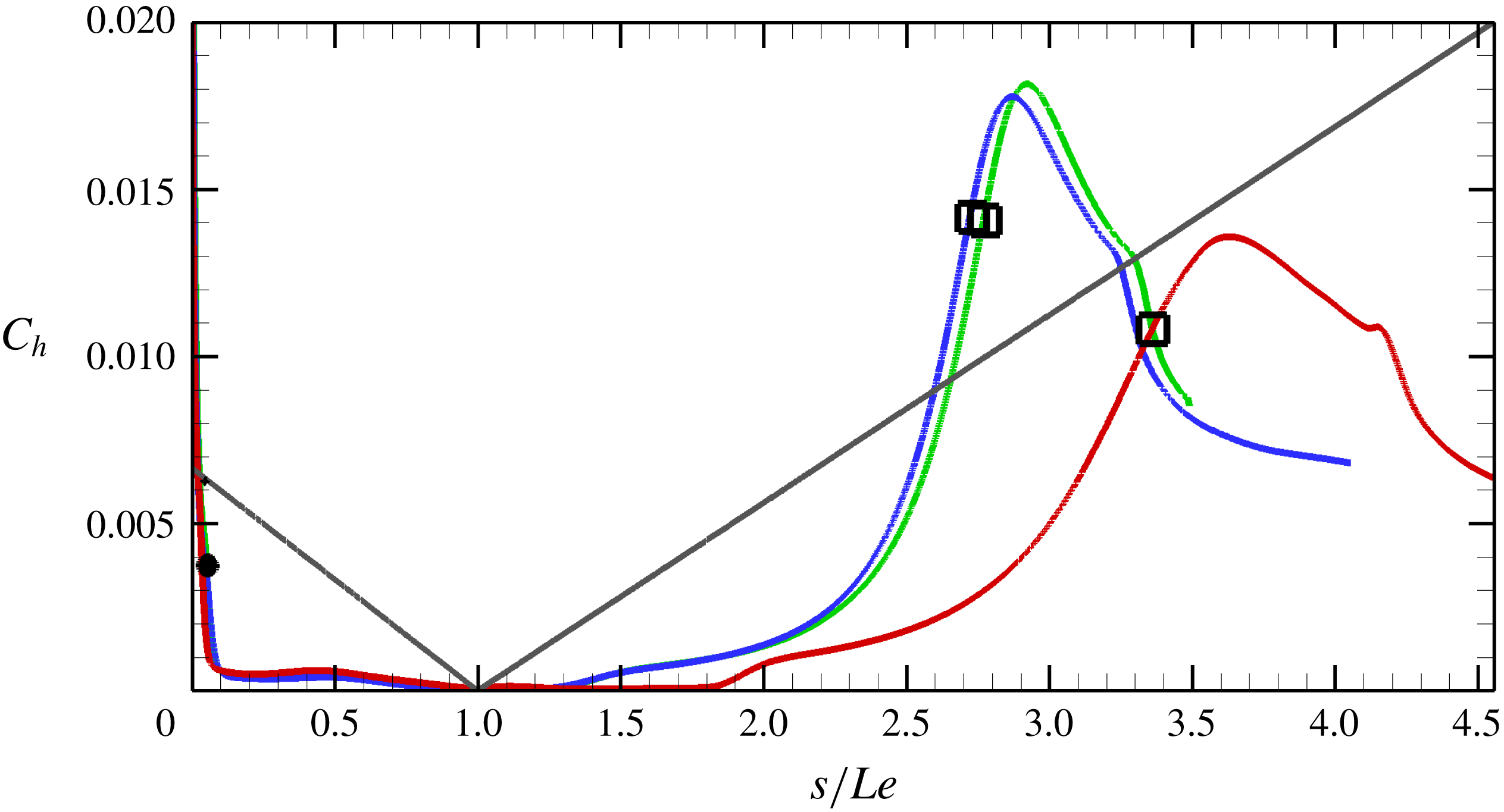
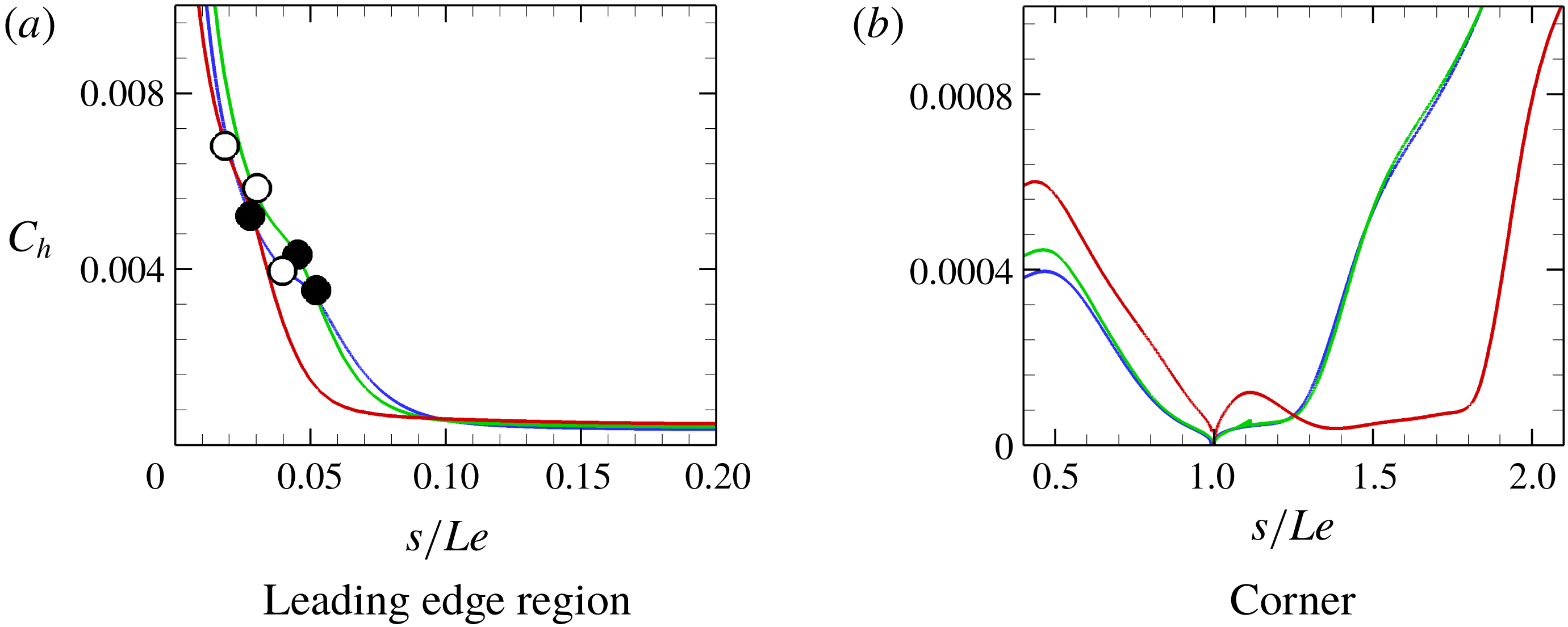
Bluntness effect on the global heat flux distribution is shown in figure 15. Magnified views of these data near the leading edge and corner regions are shown in figures 16(a) and 16(b), respectively. In the figures, we note only a small difference in the heat flux distribution of the sharp and small bluntness cases. In figure 16(a), also, it appears that bluntness reduces the severity of the ‘knee’ seen at the beginning of the interaction. It is worth noting that this particular feature also resembles the effect of wall temperature on the heat flux knee in a leading edge separation configuration shown in Khraibut et al. (Reference Khraibut, Gai, Brown and Neely2017).
We also note that while there is a significant reduction in peaks of the heat flux with increasing bluntness (figure 15), bluntness effect on the heat flux values near the separation and corner regions (figure 16 a,b) differs. Figure 16(a), for example, shows a reducing effect near separation and downstream of the corner, while figure 16(b) shows an increasing effect of bluntness on the heat flux values upstream of the corner.
Bluntness effects on the surface heat flux
 $C_{h}$
distribution. Green line: sharp leading edge; blue line: small blunt leading edge (
 $r=15~\unicode[STIX]{x03BC}\text{m}$
); red line: large blunt leading edge (
 $r=100~\unicode[STIX]{x03BC}\text{m}$
); grey line: surface. Filled circles: separation; open squares: reattachment.

Bluntness effects on the heat flux
 $C_{h}$
distribution near the corner. Green line: sharp leading edge; blue line: small blunt leading edge (
 $r=15~\unicode[STIX]{x03BC}\text{m}$
); red line: large blunt leading edge (
 $r=100~\unicode[STIX]{x03BC}\text{m}$
). Filled circles: separation; open circles: beginning of interaction.

The present numerical results have been validated by limited surface pressure measurements taken in T-ADFA. Details of the experimental procedures, model and calibration are given in Khraibut (Reference Khraibut2018). It should be noted that these measurements were only possible along the compression surface in these experiments considering both short length of surface
 $Le$
(expansion surface) and small leading edge thickness (
 $r=15~\unicode[STIX]{x03BC}\text{m}$
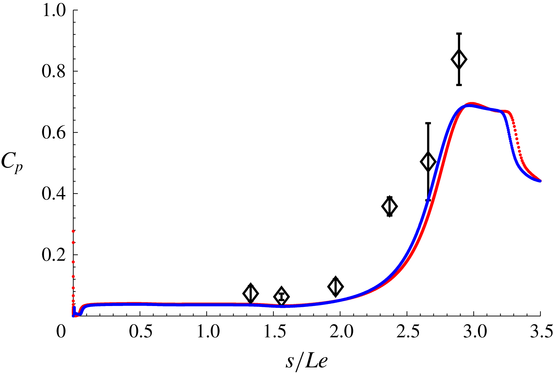
) of the model. Comparison of the numerical results for both the sharp and small bluntness cases and the experimental data is shown in figure 17.
It should be pointed out that Tumuklu, Levin & Theofilis (Reference Tumuklu, Levin and Theofilis2018) have also carried out similar simulations of the same geometry and flow conditions but using the DSMC method (SMILE code). Their simulations, which are time-accurate, were compared to the experimental data. Tumuklu et al. (Reference Tumuklu, Levin and Theofilis2018) showed results at both 1.25 and 5 ms, noting that 1.25 ms is closer to the actual experimental test time of 1 ms. At 1.25 ms, their pressures showed good agreement with experimental data, but their later time solutions indicated a final steady state at 5 ms, which is beyond the experimental times. Given their solution at 5 ms and our steady-state solutions, good agreement was seen. While their findings go to show that the experiments were not fully steady, flow in the experiments can be best described as quasi-steady. This is further supported by a maximum of 22 % difference between steady-state simulations and the experimental measurements.
Validation of surface pressures on the compression surface of the leading edge separation model. Red: sharp leading edge; blue:
 $r=15~\unicode[STIX]{x03BC}\text{m}$
; symbols: experimental data shown with error bars.

4.3 Displacement-bluntness similitude parameter
Based on the analysis given in Cheng et al. (Reference Cheng, Hall, Golian and Hertzberg1961), Holden (Reference Holden1971), who conducted intensive experiments on the flat-plate compression corner geometry, used Cheng’s displacement-bluntness parameter (
 $\unicode[STIX]{x1D6FD}=\unicode[STIX]{x1D712}_{\unicode[STIX]{x1D716}}/\unicode[STIX]{x1D705}^{2/3}$
) to classify bluntness effects on hypersonic separated regions. Various bluntness values and wedge angles were investigated in Holden’s experiments. The angles however were sufficient enough to cause incipient to moderate separations so that the boundary layer in these experiments can be described as fully developed prior to separation. Holden notably found that small values of
 $\unicode[STIX]{x1D6FD}$
reduce the size of the separated region, while large values of
 $\unicode[STIX]{x1D6FD}$
increase the size of separation. Holden, more importantly, attributed the decrease in the length of separation with smaller
 $\unicode[STIX]{x1D6FD}$
(i.e. larger bluntness) to a significant decrease in both the local Mach and Reynolds numbers prior to separation over viscous interactions. The diminishing effect of bluntness with increased
 $\unicode[STIX]{x1D6FD}$
was attributed to dominant viscous effects.
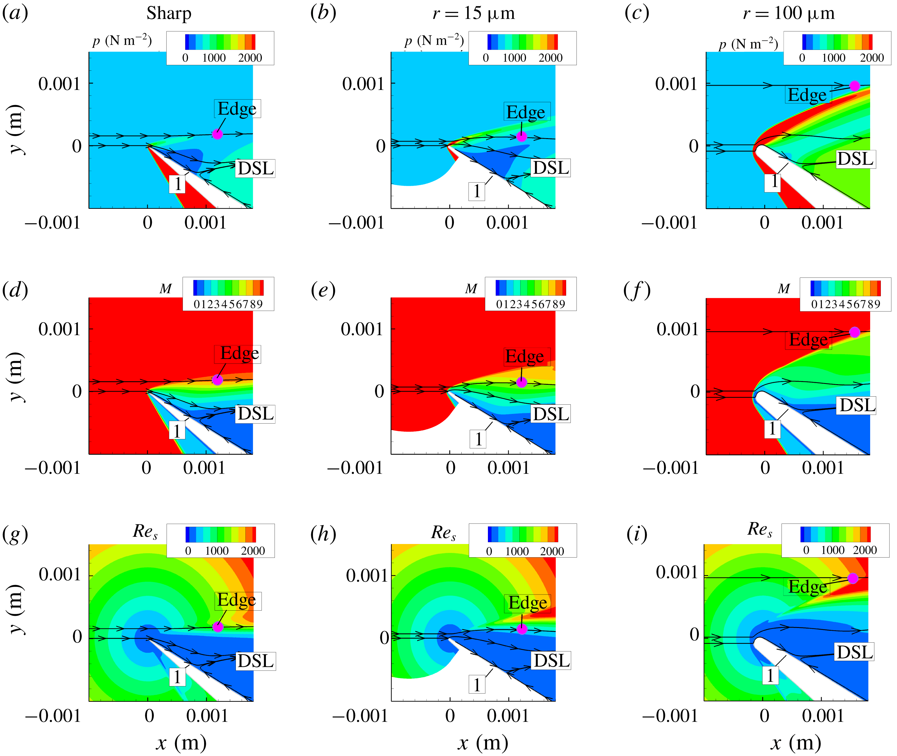
In figure 18, local flow properties just before separation (pressure, Mach number and local Reynold number
 $Re_{s}$
) are shown to demonstrate the effect of bluntness on these properties and on the location of separation. From the above discussion, it becomes clear that the displacement-bluntness parameter
 $\unicode[STIX]{x1D6FD}$
is really a measurement of the competing effects of viscous interaction and pressure effects on the size of separation, wherein increasing the former with respect to the latter increases the size of separation while the opposite reduces the size of separation. This is further manifested, in the present results (see figure 12), in the initial reduction in size of the separated region with the introduction of small bluntness (blue line) to a leading edge from an ideally sharp case (green line). This can be explained in that when the leading edge is ideally sharp, the flow is purely viscous-dominated, but when a small bluntness is added to the leading edge, it initiates favourable effects of bluntness in delaying separation and the reduction of the separation size.
Effect of bluntness on local flow properties just before separation, where DSL is the dividing streamline defining separation; ‘1’ is the beginning of pressure rise, the pink dot is located at the edge of the boundary layer as determined from streamwise velocity
 $u$
profile at ‘1’, and
 $p$
,
 $M$
and
 $Re_{s}$
are the pressure Mach number and Reynolds number along the surface, respectively.

To further highlight the relative significance of the inviscid pressure field created by the blunt leading edge and induced pressure field due to viscous boundary layer growth, we consider another perspective. As pointed out in Hayes & Probstein (Reference Hayes and Probstein1959), when the Reynolds number based on the leading edge thickness
 $Re_{t}$
and free-stream conditions is quite small, viscous effects are dominant, but when it is large the inviscid pressure field starts to prevail over viscous effects. Values of
 $Re_{t}$
for the small and large bluntness cases considered in this study are 20.1 and 134, respectively. Correspondingly, the smaller bluntness makes negligible difference to the flow downstream compared to the sharp leading edge, while the larger bluntness has a significant effect on the flow downstream.
Similar condition for bluntness effects was shown by Stollery (Reference Stollery1972), who describes a sharp leading edge that satisfies
 $$\begin{eqnarray}\displaystyle Re_{t}\ll M^{3}/\bar{\unicode[STIX]{x1D712}}^{1/2}, & & \displaystyle\end{eqnarray}$$
where
 $\bar{\unicode[STIX]{x1D712}}$
is the hypersonic viscous interaction parameter. For the present flow conditions, (4.4) becomes
 $$\begin{eqnarray}\displaystyle Re_{t}\ll 462, & & \displaystyle\end{eqnarray}$$
so, clearly, the present bluntness cases considered in the study are of the sharp type and bluntness effects are not expected to be dominant.
Furthermore, careful examination of Holden’s data shows that when
 $0.5<\unicode[STIX]{x1D6FD}<2$
, the change in size of separation
 $L_{sep}$
(distance between ‘R’ and ‘S’) is generally quite small (in the region where
 $\unicode[STIX]{x1D6FD}$
is between 1 and 2, there is a small decrease in the size of separation), and when
 $\unicode[STIX]{x1D6FD}>2$
, the size of separation is independent of
 $\unicode[STIX]{x1D6FD}$
.
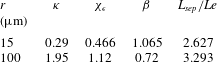
Calculations of
 $\unicode[STIX]{x1D6FD}$
are given in table 10 for both the small and large blunt leading edge cases. It is worth pointing out that the original formulation of hypersonic similitude solutions by Cheng et al. (Reference Cheng, Hall, Golian and Hertzberg1961) assumes a Blasius boundary layer prior to separation so that the shear constant
 $\unicode[STIX]{x1D706}=0.332$
. In the present case, where separation occurs close to the leading edge and as the boundary layer is still developing (non-Blasius), values of the shear constant must be adjusted based on local properties. Note also that taking the local values will account for the effect of the incidence angle on the boundary layer development. Parameters
 $\unicode[STIX]{x1D705}$
,
 $\unicode[STIX]{x1D712}_{\unicode[STIX]{x1D716}}$
and
 $\unicode[STIX]{x1D6FD}$
and their corresponding effect on length of separation
 $L_{sep}$
are all shown in the table.
In line with the analysis of Hayes & Probstein (Reference Hayes and Probstein1959) and Stollery (Reference Stollery1972), table 10 shows that
 $\unicode[STIX]{x1D6FD}$
of 1.065 for
 $r=15~\unicode[STIX]{x03BC}\text{m}$
and
 $\unicode[STIX]{x1D6FD}$
of 0.72 for
 $r=100~\unicode[STIX]{x03BC}\text{m}$
also fall within the small bluntness category given by Holden (Reference Holden1971) (
 $0.5<\unicode[STIX]{x1D6FD}<2$
). Contrary to the trend seen by Holden, however, an increase, rather than a decrease, in the size of separation (by 22 %) is observed as leading edge bluntness is increased from
 $15$
to
 $100~\unicode[STIX]{x03BC}\text{m}$
in the present case. A possible explanation for this could be in that, unlike a flat-plate boundary layer as in Holden’s experiments, in leading edge separation, the incoming boundary layer separates before it fully develops, so although both bluntness cases considered in the present study are ‘small’ in terms Holden’s criterion, their behaviour on separation is quite different. This, more importantly, also shows that under leading edge separation and present flow conditions, the size of the separated region is more sensitive to
 $\unicode[STIX]{x1D6FD}$
than in the case of flat-plate compression corner geometry.
Bluntness effects on the displacement-bluntness parameter
 $\unicode[STIX]{x1D6FD}$
and the length of separation
 $L_{sep}/Le$
.

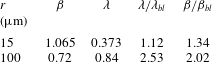
The effect of a non-Blasius boundary layer (i.e. a not fully developed boundary layer) prior to separation is seen in table 11 by values of
 $\unicode[STIX]{x1D712}_{\unicode[STIX]{x1D716}}$
, which is the hypersonic viscous interaction parameter modified to account for wall enthalpy. We note that although
 $\unicode[STIX]{x1D705}$
increases with bluntness, its effect is outweighed by an increase in the parameter
 $\unicode[STIX]{x1D712}_{\unicode[STIX]{x1D716}}$
, which leads overall to an increase in
 $\unicode[STIX]{x1D6FD}$
. In the table, the overall effect of boundary layer growth prior to separation (through the shear constant
 $\unicode[STIX]{x1D706}$
) on
 $\unicode[STIX]{x1D6FD}$
can be determined by the ratio
 $\unicode[STIX]{x1D6FD}/\unicode[STIX]{x1D6FD}_{bl}$
showing the deviation of the current case from a fully developed Blasius boundary layer. In this ratio, subscript ‘
 $bl$
’ refers to Blasius. By examining the table, we observe an increase in the value
 $\unicode[STIX]{x1D706}$
(by a factor of 1.12 for
 $r=15~\unicode[STIX]{x03BC}\text{m}$
and 2.53 for
 $r=100~\unicode[STIX]{x03BC}\text{m}$
) caused by the leading edge separation compared to the Blasius case. This seems to also lead to an increase in the value of
 $\unicode[STIX]{x1D6FD}$
(by a factor of 1.34 for
 $r=15~\unicode[STIX]{x03BC}\text{m}$
and 2 for
 $r=100~\unicode[STIX]{x03BC}\text{m}$
) in the case of leading edge separation over the Blasius case. This is important to note because it suggests that the leading edge separation tends to further suppress favourable effects of bluntness in delaying separation.
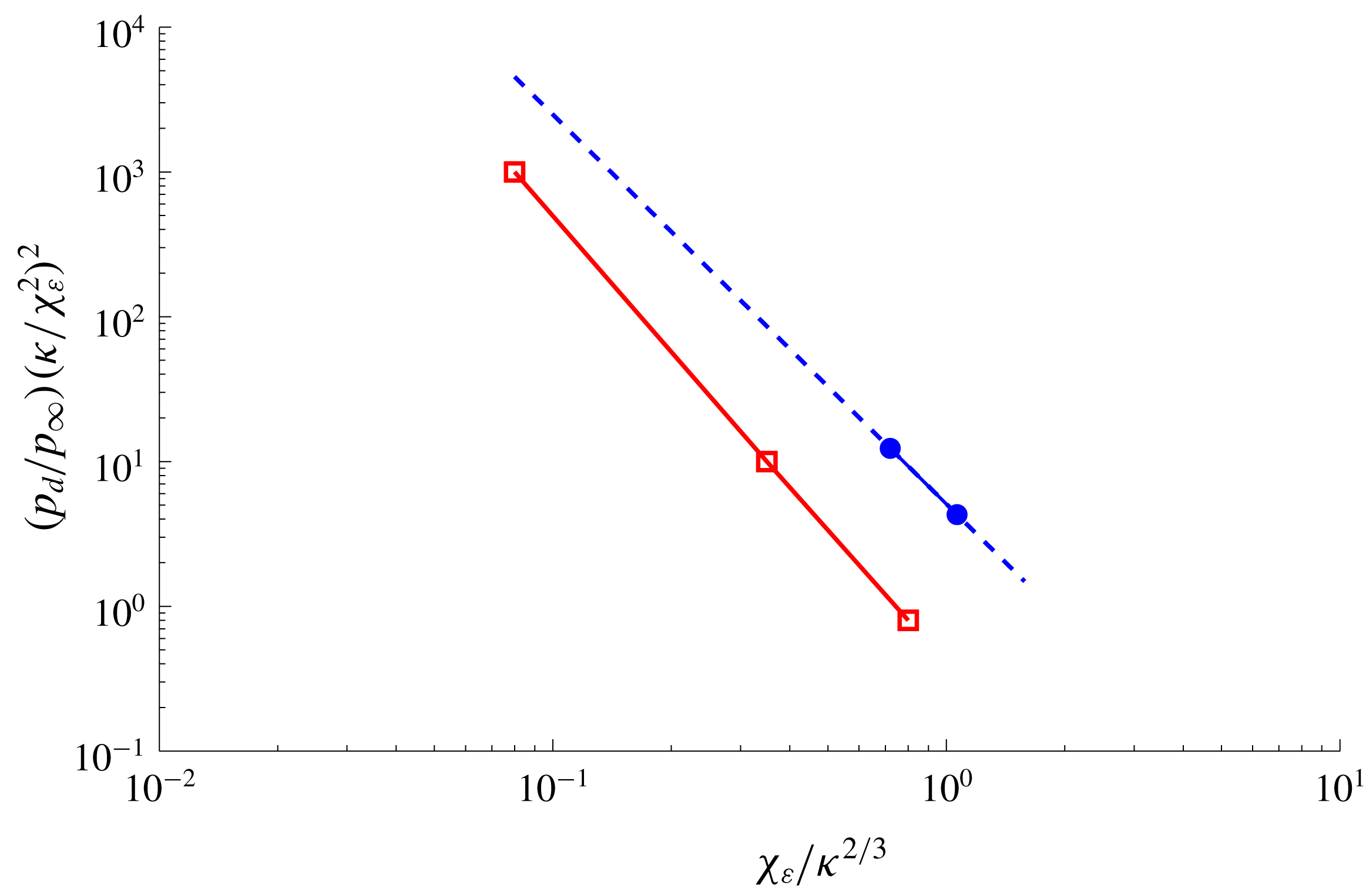
Figure 19 shows a correlation between plateau pressure parameter
 $(p_{d}/p_{\infty })(\unicode[STIX]{x1D705}/\unicode[STIX]{x1D712}_{\unicode[STIX]{x1D716}}^{2})^{2}$
and
 $\unicode[STIX]{x1D6FD}$
in the fashion of Holden (Reference Holden1971). In the figure, the right-hand shift of the leading edge separation data (filled blue circles) indicates an opposite trend to that of Holden finding a decrease in plateau pressure with increasing bluntness (i.e. reduction of
 $\unicode[STIX]{x1D6FD}$
). The present results can be verified by the surface pressure data given in figure 5(a–c).
Effect of a non-Blasius boundary layer on the displacement-bluntness parameter
 $\unicode[STIX]{x1D6FD}$
.

Bluntness effects on the plateau pressure parameter
 $(p_{d}/p_{\infty })(\unicode[STIX]{x1D705}/\unicode[STIX]{x1D712}_{\unicode[STIX]{x1D716}}^{2})^{2}$
. Blue filled circles: present data; red open squares: experimental data of Holden (Reference Holden1971) for the flat-plate compression ramp configuration; dashed line: extension of the slope of the present data.

4.4 Effect of bluntness on RBL and transverse gradients
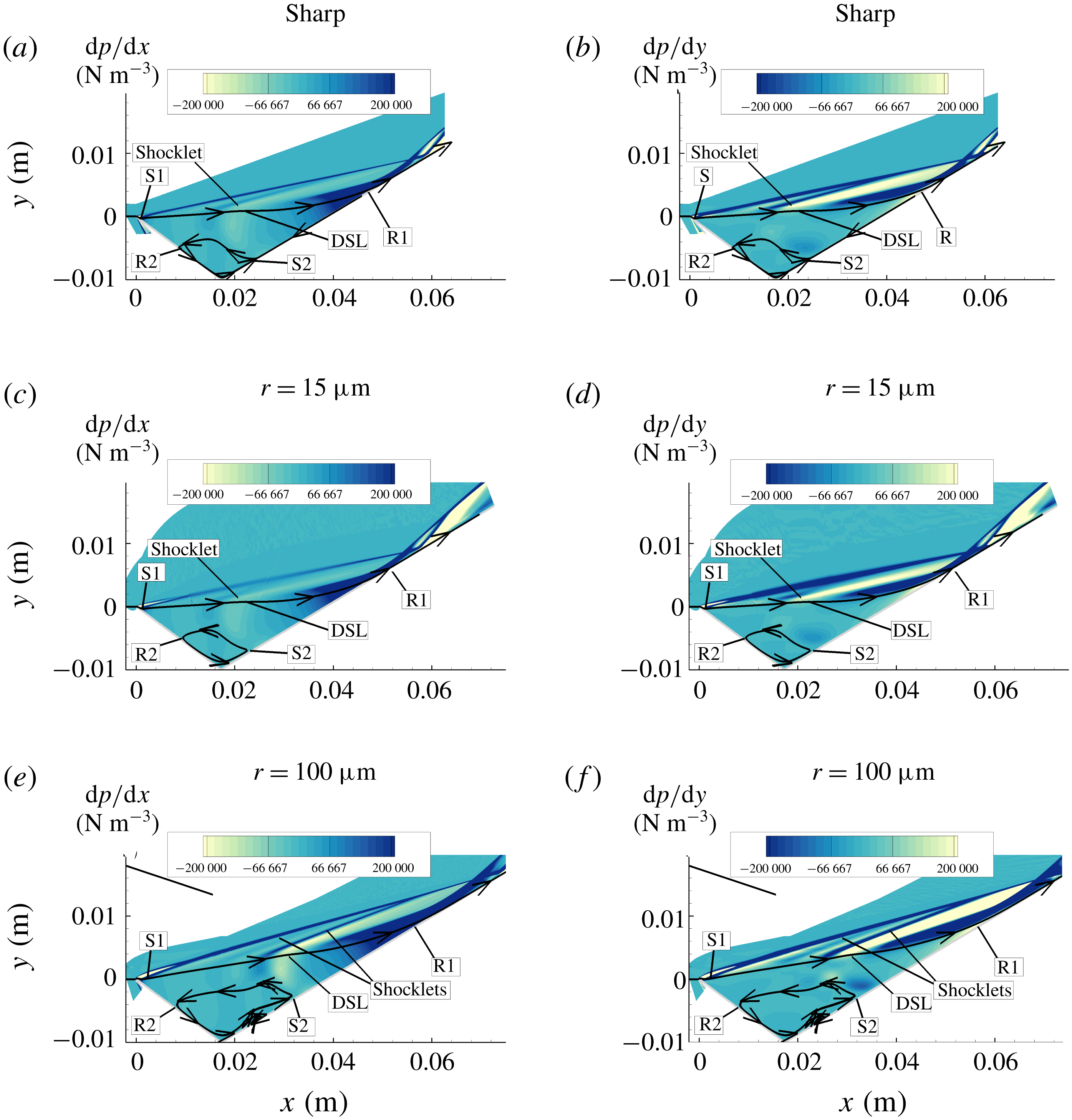
An attempt to explain the development of multiple vortices in the context of streamwise and transverse pressure gradients
 $\text{d}p/\text{d}x$
and
 $\text{d}p/\text{d}y$
is given in this section. These gradients are shown for the sharp leading edge in figure 20(a,b), small bluntness case in figure 20(c,d) and large bluntness case in figure 20(e,f). They are also considered as it is possible that they contribute mostly, as suggested by Neiland et al. (Reference Neiland, Sokolov and Shvedchenko2009), to the development of multiple vortices within a separated region. In figure 20, it is noted that the present results agree with those of Neiland in that such gradients are predominantly present in the reattachment region close to ‘R1’, where the RBL develops and separates at ‘S2’ and forms secondary separations within the main separation. The figure further shows some shocklets, which emerge from within the shear layer. The number of shocklets is found to correspond to the number of multiple vortices within the separated region, which are vortex 2 in the sharp/small bluntness cases, and vortices 3 and 4 in the large bluntness case (see figure 10). These figures also show that increasing bluntness increases the strength of the streamwise and transverse pressure gradients, which promotes the fragmentation of vortices. These figures also show Type VI shock–shock interaction for both the sharp and blunt leading edge cases and the shocklets intersect the incoming shock wave from the leading edge region.
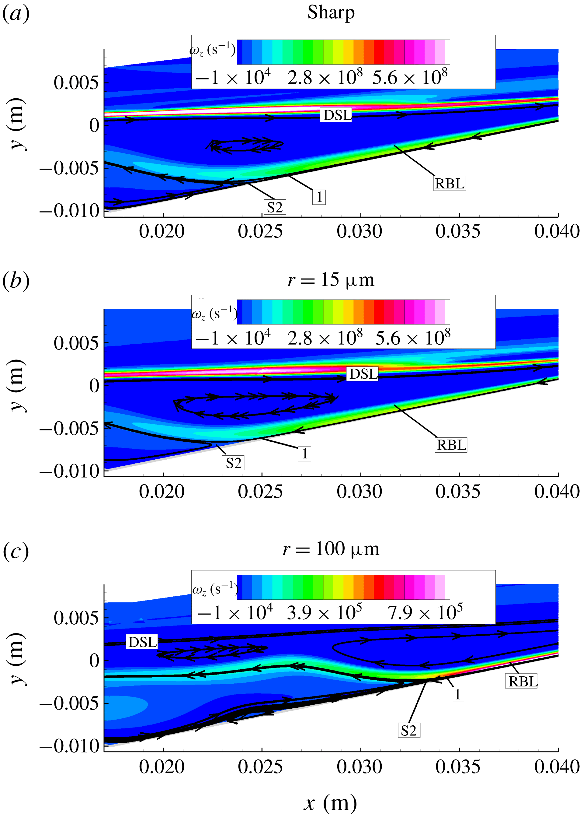
In figure 21, vorticity contours
 $\unicode[STIX]{x1D714}_{z}$
for both the sharp and blunt leading edge case provide some insight into the development of the RBL, where ‘S2’, mentioned earlier, is the separation location of the RBL, and ‘1’ is the location just upstream of ‘S2’. Clearly, the figure shows that the RBL profoundly affects the flow behaviour within the separated region.
Bluntness effects on streamwise
 $\text{d}p/\text{d}x$
and transverse
 $\text{d}p/\text{d}y$
pressure gradients.

Bluntness effects on RBL based on the vorticity contours
 $\unicode[STIX]{x1D714}_{z}$
.

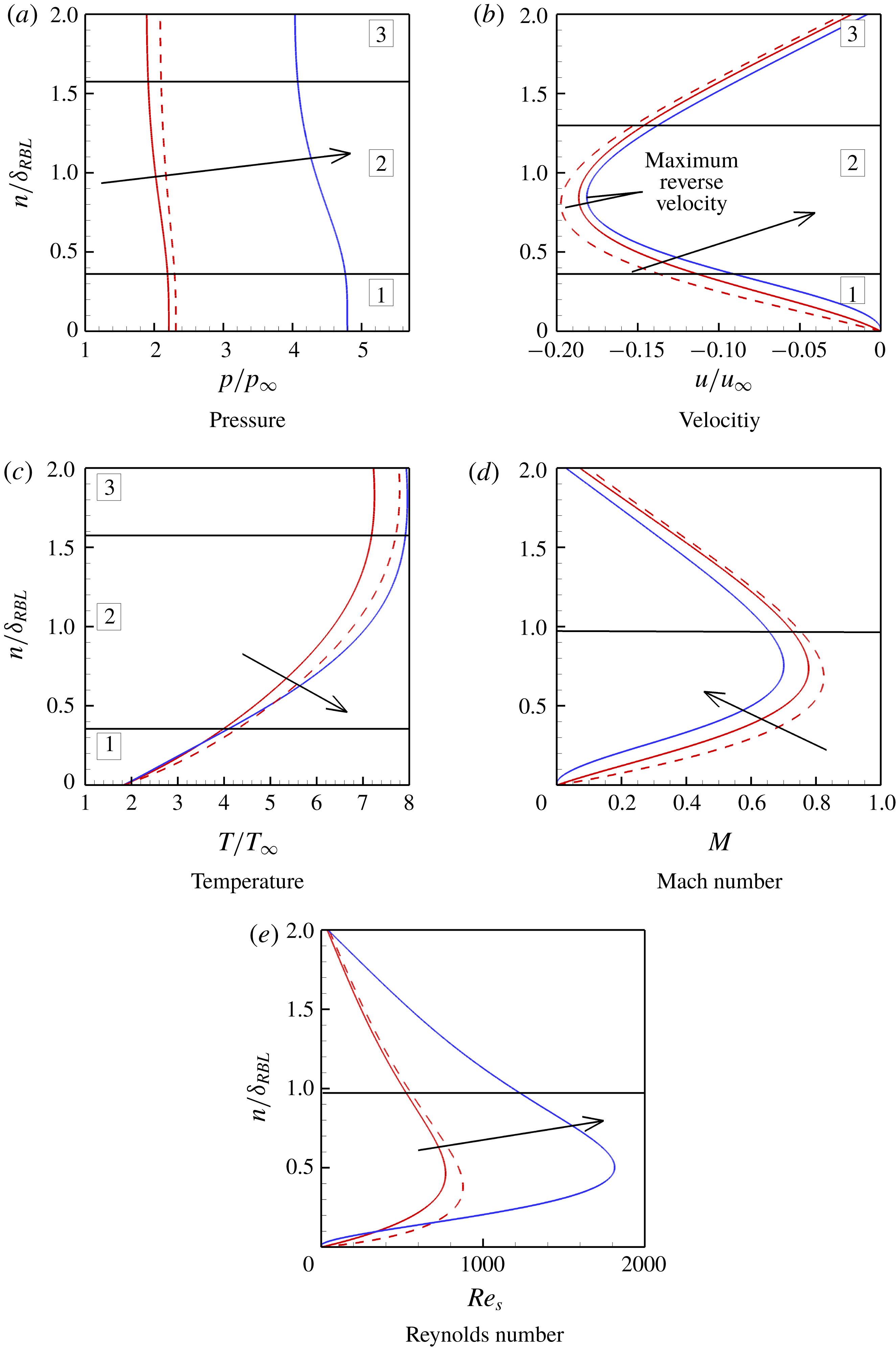
Bluntness effects on RBL profiles. Dashed red line: sharp leading edge; solid red line: small bluntness leading edge (
 $r=15~\unicode[STIX]{x03BC}\text{m}$
); solid blue line: large bluntness leading edge (
 $r=100~\unicode[STIX]{x03BC}\text{m}$
). Here,
 $n/\unicode[STIX]{x1D6FF}_{RBL}$
is the normal distance from the wall at location ‘1’. Arrows point in the direction of increased bluntness, while the numbers and solid black lines refer to the distinct regions within these profiles.

These characteristics are shown next by examining the pressure, velocity and temperature profiles normal to the surface as at location ‘1’ (figure 21). The profiles are shown, respectively, in figures 22(a) to 22(c), where they have been normalised by the free-stream values (subscript ‘
 $\infty$
’), and surface normal distance
 $n$
is normalised by the RBL thickness
 $\unicode[STIX]{x1D6FF}_{RBL}$
. (Parameter
 $\unicode[STIX]{x1D6FF}_{RBL}$
is inferred from the vorticity contours provided in figure 21 at ‘1’.) It should also be noted that the normal distance has been extended to twice the RBL thickness into the main separation to provide an additional insight. The figures show that reverse boundary layer profiles of the sharp case (dashed red lines) and small bluntness case are generally similar, so that the present discussion focuses mainly on the results of small and large bluntness cases. In these figures, the arrows point in the direction of increased bluntness, while solid lines, which separate regions 1, 2 and 3, denote distinct regions within these profiles.
Considering pressure profiles (figure 22 a) first, it was noted that normal pressure gradients exist within the RBL, mainly in region 2 of the figure. These gradients were also found to increase with increased bluntness. The figure further showed that the increase in the pressures in the large bluntness case, by more than a factor of two, is consistent with the reduction of RBL thickness seen earlier in figure 21.
The velocity profiles (figure 22
b), on the other hand, reveal further important features concerning the structure of the RBL. For instance, the profiles show that close to the wall in region 1, the velocity reduces in magnitude but the slope of the curve, which relates to the vorticity, increases with increasing bluntness. The velocity profile was further found to vary linearly with
 $n$
in region 1 for both the sharp/small bluntness cases (i.e. of constant vorticity), while in the large bluntness cases, it shows a slightly nonlinear increase (produces vorticity) with
 $n$
. These profiles show a maximum reverse velocity in region 2, which reaches 20 % of the free-stream value in the case of small bluntness. The maximum reverse velocity is seen to slightly decrease with increased bluntness. Outside the boundary layer, in region 3 (the main separation), the velocity variation is consistent with the outer rotational flow of constant vorticity.
Temperature profiles (figure 22
c) across the RBL demonstrate the existence of normal thermal gradients in regions 1 and 2 of the boundary layer, for all cases considered, while in region 1 the magnitude of these profiles does not seem to be significantly affected by leading edge bluntness. The outer temperature profiles, in region 3, which occur in the main vortex, in this figure, also show negligible or small temperature variation with
 $n$
(nearly isothermal).
Figure 22(d,e) shows the Mach number
 $M$
and Reynold number
 $Re_{s}$
profiles across the RBL, where
 $Re_{s}$
, in figure 22(e), is based on the wetted distance
 $s$
and local flow properties, and solid lines in both panels denote the edge of the boundary layer.
Considering the Mach number profiles first, figure 22(d) shows a generally subsonic to transonic variation for all leading edge cases. The larger Mach number values were found to occur in the sharp/small bluntness cases and the Mach number values weer found to reduce with bluntness.
Reynolds number profiles (figure 22 e), on the other hand, show the opposite effect of bluntness on the magnitude and a larger bluntness yields larger Reynold numbers across the boundary layer. It is further noted that, while the velocity profiles show a decrease with an increase in the bluntness (figure 22 b), the Reynolds numbers show a decrease with increased bluntness. Such an effect can be attributed to higher viscosities expected in the outer region 3 of the boundary layer compared to the inner regions 1 and 2, which are consistent with the temperature profiles shown in figure 22(c).
Overall, it is clear that leading edge bluntness influences the recirculation region and the reattachment process, and, through bluntness, the development of the RBL. This in turn induces transverse and streamwise gradients which eventually leads to the separation of the reverse flow boundary, and hence the appearance of multiple vortices within a separated region.
5 Summary and conclusions
A numerical investigation into bluntness effects on laminar hypersonic leading edge separation has been presented. Although the bluntness cases studied here fall into the category of ‘small’ bluntness in terms of Holden’s characterisation of bluntness of the leading edge, some significant differences were observed. While the smaller of the two bluntness cases studied was largely similar to the ideal sharp case, albeit with a small reduction in the size of the separated region, the larger bluntness case showed a considerable increase in the size of the separated region, which is opposite to the trend seen in Holden’s experimental data. It is suggested that this difference is mainly due to the leading edge separation geometry, unlike Holden’s experiments, which were conducted with a flat-plate compression corner geometry. Another interesting finding in the study is that the leading edge separation negates the favourable effects of bluntness on separation. It also makes the length of separation to be more sensitive to the displacement-bluntness similitude parameter of Cheng.
We also report, perhaps for the first time, the presence of multiple vortices within the main separated region and the effect of bluntness on the formation of these vortices. It is proposed that the origin of these vortices lies in the RBL which develops in the reattachment region. Properties of the RBL have been investigated to show how transverse gradients in the RBL will lead to secondary vortices. It was found that increase of bluntness also increases these gradients in the RBL, which promote fragmentation of these vortices. Outside the RBL, the velocity profile was found to be consistent with the near-inviscid rotational flow of constant vorticity.
Acknowledgements
We are grateful to the Australian Research Council (ARC) for supporting our work under grant DP-140100842. We would like to acknowledge the National Computing Infrastructure (NCI) for providing us with the computational time required for the simulations. Finally, our sincere thanks to Professor G. Candler at the University of Minnesota for granting us permission to use US3D.