4.1. Overview of flow structure

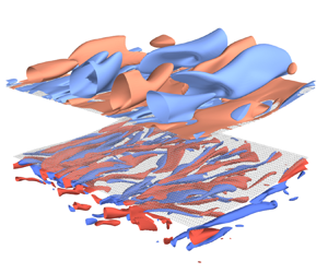
An overview of the simulated wave motion and the resulting turbulence field is presented. Figure 3 is the three-dimensional plot of the streamwise ($x$ component) vorticity component in the AW-ctrl case at $t=1200{\rm \pi}$ showing the elongated vortex structure. This is consistent with the streak structure observed in the laboratory experiment by Savelyev et al. (Reference Savelyev, Maxeiner and Chalikov2012). The vortices are present both in the water and air domains, but their typical spatial scale is larger in the air side because of the larger kinematic viscosity value there. These turbulent vortices developed over the time scale of $O(100)$ wave periods, as described in § 4.2.

Figure 3.

Three-dimensional plot of the turbulence field of the AW-ctrl case at $t=1200{\rm \pi}$. The curved grey surfaces denote the interface, and the air domain is artificially lifted for visibility. Red and blue surfaces denote contours of $x$-component vorticity ${\partial w }/{\partial x }-{\partial v }/{\partial z }$ ($\pm 0.013$ in the air and $\pm 0.020$ in the water), and the red (blue) surfaces show the positive (negative) contours. Waves propagate towards the $x$ direction.

The velocity field in the AW-ctrl case is shown in figures 4 and 5. The instantaneous velocity field is dominated by the wave orbital motion, which is nearly uniform in the $y$ direction, so the deviation from the $y$ average along constant $x^*$ and $z^*$ lines is considered as the turbulence field. Hereinafter, prime is used to denote the turbulence component:

(4.1)\begin{equation} \varphi'(x^*,y^*,z^*,t^*)\equiv \varphi(x^*,y^*,z^*,t^*) - \langle\varphi\rangle_y(x^*, z^*, t^*), \end{equation}

where $\varphi$ denotes an arbitrary field and

(4.2)\begin{equation} \langle\varphi\rangle_y(x^*, z^*, t^*)\equiv \frac{1}{L_y}\int_0^{L_y} \varphi(x^*,y^*,z^*,t^*) \,{\rm d} y^* \end{equation}

is the along-crest average.

Figure 4.

Vertical cross-section of the flow field of the AW-ctrl case at $t=2400{\rm \pi} $: (a) $\langle u\rangle _y$; (b) $\langle v\rangle _y$; (c) $\langle w\rangle _y$; (d) $\langle u^{\prime 2}\rangle _y$; (e) $\langle v^{\prime 2}\rangle _y$; ( f) $\langle w^{\prime 2}\rangle _y$. Note that the colour range is different for air and water sides in the along-crest variance plots.

Figure 5.

Top view of $u'$, $ v '$ and $w'$ obtained in the AW-ctrl case at $t=2400{\rm \pi}$: (a–c) distributions on $z^*=0.2$ (air) and (d–f) distributions on $-0.2$ (water).

Figure 4 shows the $x$–$z$ vertical section of the velocity field at $t/2{\rm \pi} =1200$. Since $\eta$ is almost uniform in the $y$ direction, $\langle \eta \rangle _y$ is used as the interfacial shape. Figure 4(a–c) show that the crest-averaged velocity field is dominated by the wave orbital motion. Although it is invisible in the present plotting, the air-side $\langle u\rangle _y$ sharply adjusts to the water-side value near the interface. This will be further demonstrated in § 4.3. The along-crest variance of velocity components shows that the horizontal components of the turbulence component are located near the interface. The vertical component $\langle w^{\prime 2}\rangle _y$ is also concentrated near the interface in the water side, but it is centred at the middle of the domain in the air, representing the large vertical scale of vortices in the air side.

Figure 5 shows the horizontal distribution of $u'$, $ v '$ and $w'$ at both air side (upper row, $z^*=0.2$) and water side (lower row, $z^*=-0.2$). The flow structure is elongated in the wave propagation direction in both the air and water sides, and its spatial scale is finer for the water side because of its smaller viscosity. On the water side, the downwelling part $w'<0$ is often associated with the down-wave velocity $u'>0$, which is consistent with the typical structures of the LCs (Leibovich Reference Leibovich1983) and the turbulence produced in water-only wave resolving simulations (Tsai et al. Reference Tsai, Lu, Chen, Dai and Phillips2017). The air-side flow shows an upsidedown LC-like structure in that the strong streamwise current region ($u'>0$) corresponds well with the convergence zone ${\partial v '}/{\partial y }<0$ and the upwelling zone $w'>0$. This is understandable because the wave-driven airflow (figure 7d) has the negative shear ${\partial \bar {u}^{E}}/{\partial z }<0$, and the shear of the air-side Stokes drift ${\partial u ^{St}}/{\partial z }=-2a^2 {\rm e}^{-2z} < 0$ has the same sign. This results in CL2 instability (Leibovich Reference Leibovich1983), producing the roll structure in the air side as well. The W-ctrl case also showed a turbulent flow pattern similar to the water side of the AW-ctrl case, and their difference in turbulence intensity is discussed in § 4.2.

4.2. Temporal evolution of flow field

Here, the temporal evolution of the flow field is described. First, figure 6 shows the temporal variation of the wave amplitude. The wave amplitude is evaluated as $a(t)=(2\overline {\eta ^2})^{1/2}$, where the overline denotes horizontal average. Both in the AW and W cases, the decay rate is almost identical with and without turbulence. The simulated decay rate followed the linear theory of Dore (Reference Dore1978) (AW) and Lamb (Reference Lamb1932) (W) well, indicating the prevalence of linear dynamics. The simulated decay rate of both the AW-ctrl and AW-noturb cases exceeded the theoretical prediction slightly, although this deviation diminished with a higher vertical resolution near the interface on the air side. This suggests that the air-side Stokes layer is playing a central role in the energy dissipation, and it needs to be properly resolved when we focus on its role. With that caveat in mind, we proceed with the present resolution, as the enhanced wave decay predicted by the linear theory is mostly reproduced.

Figure 6.

Temporal change of wave amplitude $a(t)=\sqrt {2\overline {\eta ^{2}}}$ normalised with its initial value $a(0)$. Dashed lines denote the decay rate predicted with the linear theories (1.3) and (1.1).

As waves decay, they give up the horizontal momentum and produce a vortical current, namely, the Eulerian mean drift. The Eulerian mean drift is evaluated by first vertically interpolating the horizontal velocity field $u$ to fixed levels and then taking a horizontal average. The temporal evolution of the Eulerian mean horizontal velocity $\bar {u}^{E}(z, t)$ is shown in figure 7. The data at the vertical levels between wave crests and troughs are not plotted here. The comparison of the AW-noturb and W-noturb cases (figure 7b,c) shows that, due to the enhanced energy decay in the air–water coupling, the development of $\bar {u}^{E}$ is also accelerated in the AW case. In the air side of the AW-noturb case (figure 7a), the Eulerian mean drift develops in the down-wave direction. The drift near the interface is stronger than that in the water-side drift. However, its velocity scale is still on the order of the water-side Stokes drift $O(a^2k\sigma )$. In the realistic ocean, this is likely significantly smaller than that of the wind over the waves, which is typically on the order of the wave phase speed $O(\sigma /k)$.

Figure 7.

Vertical profiles of the Eulerian mean horizontal velocity $\bar {u}^{E}$ of the AW-noturb, AW-ctrl, W-noturb and W-ctrl cases: (a) AW-noturb, air; (b) AW-noturb, water; (c) W-noturb; (d) AW-ctrl, air; (e) AW-ctrl, water; ( f) W-ctrl. Dashed lines in (b) show the result of the one-dimensional diffusion equation (4.3).

The evolution of water-side Eulerian mean drift in the AW-noturb case is compared with the virtual wave stress theory. The one-dimensional diffusion equation below was simulated for the velocity profile $u(z,t)$ in the water side ($-H_{o}\leq z\leq 0$):

(4.3)\begin{equation} \dfrac{\partial u}{\partial{t}} = \nu_{o}\dfrac{\partial^2u}{\partial{z}^2}. \end{equation}

The upper boundary condition is provided as the virtual wave stress, $\nu _{o}({\partial u }/{\partial z })=\tau ^{vws}_{ao}$ (1.4), and the bottom boundary is assumed as free-slip. Since the amplitude time series was well followed by the linear theory (figure 6), the wave amplitude $a(t)$ used in $\tau ^{vws}_{ao}$ is assumed to exponentially decay with time as $a(t) = a(0){\rm e}^{-\gamma _{ao} t}$. The result is shown as the dashed lines in figure 7(b), which mostly overlaps with the AW-noturb simulation result.

In the three-dimensional cases, turbulence alters the velocity profile by carrying horizontal momentum away from the interface. As a result, velocity profile $\bar {u}^{E}$ shows weaker vertical shear in both air and water sides (figure 7d–f).

Veron & Melville (Reference Veron and Melville2001) derived a similarity solution of the wind-driven sheared current in the water-side based on the one-dimensional diffusion equation (4.3) subject to a constant wind stress $\tau$. Wu & Deike (Reference Wu and Deike2021) conducted a two-dimensional DNS of the wind–wave growth under the influence of viscosity and confirmed that the wind-induced drift current $\bar {u}^{E}(z,t)$ falls into a single curve if the depth and the velocity are scaled with $\sqrt {\nu _{o} t/8}$ (under our non-dimensionalisation $\sqrt {t/8{\textit {Re}}_{o}}$) and $U_0(t)\equiv \bar {u}^{E}(0,t)$, respectively. Figure 8(b,c) show the temporal evolution of the Eulerian current profile scaled as previously. Here, the velocity scale $U_0(t)$ is evaluated as (Veron & Melville Reference Veron and Melville2001; Wu & Deike Reference Wu and Deike2021)

(4.4)\begin{equation} U_0(t) = \frac{2}{\sqrt{\rm \pi}}\tau\sqrt{\frac{t}{{\textit{Re}}_o}},\end{equation}

and $\tau =\tau ^{vws}_{ao}(0)$ and $\tau =\tau ^{vws}_{o}(0)$ for the AW-ctrl/noturb and W-ctrl/noturb cases, respectively. The AW-noturb and W-noturb cases follow the scaling well, but in the AW-ctrl and W-ctrl cases, the shear is reduced due to turbulence, and the drift current profiles deviate from the scaling solution.

Figure 8.

Vertical profiles of the normalised Eulerian mean horizontal velocity $\bar {u}^{E}$ of the AW-noturb, AW-ctrl, W-noturb and W-ctrl cases: (a) air-side velocity profile in the AW cases; (b) water-side profile in the AW cases; and (c) water-side profile in the W cases. Solid (dashed) lines in each panel indicate the AW-noturb and W-noturb (AW-ctrl and W-ctrl) cases. Vertical coordinate is normalised with the viscous length scale $\sqrt {t/{\textit {Re}}}$. The horizontal velocity is normalised with $U_0(t)$ of (4.4) in (b,c).

On the air side, however, the drift velocity scales differently. The Eulerian current profile in the air with vertical coordinate scaled with $\sqrt {t/8 {\textit {Re}}_{a}}$ is shown in figure 8(a). Unlike on the water side, the profiles of the AW-noturb case fall into a single curve without scaling with $U_0(t)$. Therefore, the air-side drift current develops as if a Dirichlet-type boundary condition is imposed at the bottom.

Next, the temporal evolution of turbulence, characterised by deviation velocity from $y$ average $(u', v ',w')$ is compared among cases. Figure 9 shows the temporal evolution of water-side turbulent kinetic energy (TKE) and the spanwise wavelength $l_s$. TKE is defined as $(r/2)(u^{\prime 2}+ v ^{\prime 2}+w^{\prime 2})$. Temporal evolution of its vertical profile (horizontally averaged along $z^*$-surface) is shown for the AW-ctrl (figure 9a) and W-ctrl (figure 9b) cases. Turbulence arises from the near-interface layer and spreads into the water as time passes. The magnitude of turbulence is greater in AW-ctrl than in W-ctrl throughout the simulation period. Note that, even at $t/2{\rm \pi} =1200$, the turbulence has not fully reached the bottom of the water side. However, the turbulence near the interface has reached a mature stage, and the turbulence statistics no longer change rapidly. Therefore, we can expect that the flow field of AW-ctrl after $t/200{\rm \pi} \approx 500$ would well reflect the dynamics of turbulence produced by persistent wave forcing in the air–water coupled configuration.

Figure 9.

Temporal evolution of water-side turbulence statistics in the AW-ctrl, W-ctrl, AW-deepnoise and AW-ak2 cases: (a,b) vertical-temporal distribution of horizontally averaged TKE in the AW-ctrl and W-ctrl cases, respectively; (c) time series of TKE averaged over $-0.4\leq z^*\leq 0$, where the TKE of the AW-2d case is multiplied by 0.1 for visibility; (d) time series of spanwise wavenumber $l_s$ defined in (4.5) evaluated at $-0.4\leq z^*\leq 0$. Horizontal white-dashed lines in (a,b) denote $z^*=-0.4$ above which the TKE and $l_s$ in (c,d) are evaluated.

To illustrate the turbulence development in different cases more quantitatively, let us examine TKE vertically averaged over $-0.4\leq z^*\leq 0$ shown in figure 9(c). In all cases, the TKE is initially of very small magnitude (e.g. $O(10^{-7})$ in AW-ctrl), rapidly grows in the earlier stage, and then saturates, reflecting some instability mechanism at work. The onset of instability is quicker in AW-ctrl ($t/2{\rm \pi} \approx 175$) than W-ctrl ($t/2{\rm \pi} \approx 250$), and TKE magnitude of the former remains stronger than the latter throughout the simulation period. Therefore, the air–water coupling enhances the wave-induced turbulence.

To characterise the spatial scale of the turbulence, we have evaluated the TKE-weighted mean spanwise wavenumber $l_s$ following Tsai et al. (Reference Tsai, Lu, Chen, Dai and Phillips2017), as follows:

(4.5)\begin{equation} l_s(t) = \frac{\int lS(l,t) \,{\rm d} l}{\int S(l,t)\,{\rm d} l}, \end{equation}

where $l$ is the wavenumber in the $y$ direction and $S(l,t)$ is the spanwise power spectral density of turbulence velocity averaged over $0\leq x^*\leq 2{\rm \pi}$ and $-0.4 \leq z^* \leq 0$,

(4.6)\begin{align} S(l,t) = \frac{1}{0.4}\frac{1}{2{\rm \pi}}\int_0^{2{\rm \pi}}\int_{{-}0.4}^0[S_u(x^*,l,z^*,t) + S_ v(x^*,l,z^*,t) +S_w(x^*,l,z^*,t)] \,{\rm d} z^* \,{\rm d}\kern0.7pt x^*, \end{align}

where $S_u$ and so on denote the power spectral density obtained by applying the Fourier transform in the $y^*$ direction.

The temporal evolution of $l_s$ is shown in figure 9(d). Before the onset of instability, the turbulence field is dominated by the spatial scale of $l_s\approx 7$, which corresponds to the initial noise field. As the disturbance grows, vortices with relatively high wavenumbers first develop, and then the dominant spanwise scale grows ($l_s$ decreases) rapidly after the instability is saturated. At a later stage of the simulation period, the temporal development of $l_s$ is small. The AW-ctrl and W-ctrl cases show the similar temporal evolution of $l_s$, except that the time series in W-ctrl is lagged behind AW-ctrl by about 50 periods, consistent with the delay of the instability onset.

The result of the AW-deepnoise case is shown in figure 9(c,d) with a blue dashed line. The rapid growth of TKE at the onset stage and the subsequent decrease of $l_s$ observed in the AW-deepnoise case precedes the corresponding changes in AW-ctrl. As a result of the initial noise injected into all the water grid points, the initial TKE level (about $1\times 10^{-5}$) is about 300 times greater than in the AW-ctrl case. This results in an enhancement of the initial amplitude of the fastest-growing mode, so we can understand that the onset of instability occurs earlier. However, after the turbulence reached maturity, there was no clear difference between AW-deepnoise and AW-ctrl. Therefore, the statistical features of the simulated turbulence are not dependent on the initial noise structure, and only the onset timing of instability is changed.

To examine the influence of wave amplitude on the phenomenon, we have conducted an air–water coupled case with greater initial wave amplitude, $a=0.2$ (AW-a2 case). The spatial structure of turbulent velocity was similar to AW-ctrl: the vortices elongated in wave-propagation direction was observed, and the temporal evolution of turbulence statistics is shown in figure 9. Overall, the temporal evolution of turbulence is similar to the AW-ctrl case, but the onset of instability is earlier ($t/2{\rm \pi} \approx 75$). This reflects the stronger Eulerian sheared current ($\propto \tau ^{vws}_{ao}\propto a^2$) than AW-ctrl, resulting in a greater growth rate of instability. The magnitude of TKE at the mature stage (average over $600\leq t/2{\rm \pi} \leq 1200$) is about eight times greater than that of AW-ctrl.

From these results, we can make a remark on the onset time scale of wave-induced turbulence (300 periods in the AW-ctrl case). The DNS by Tsai et al. (Reference Tsai, Lu, Chen, Dai and Phillips2017) required only 10 wave periods for turbulence to develop. In their set-up, the wave slope was 0.25, which is even greater than in our AW-a2 case, and they imposed the initial noise that contains 0.1 % of the total energy. The large amplitude should lead to a strongly unstable condition, and the fraction of disturbance energy is much greater than our set-up ($O(10^{-6})\%$ for the AW-ctrl and AW-a2 cases), so the initial instability is considered to be strongly seeded. Therefore, in the simulation set-up of Tsai et al. (Reference Tsai, Lu, Chen, Dai and Phillips2017), the instability is expected to arise at an early stage after the simulation starts. Notably, the tank experiment of Savelyev et al. (Reference Savelyev, Maxeiner and Chalikov2012) also observed the turbulence growth at a similar time scale (ramp-up time of 7–10 periods followed by 6–9 periods with constant wave amplitude). Therefore, we consider that the initial noise field of our simulation design was too weak, leading to unrealistically long spinup period of $O(100)$ wave periods. However, our simulations demonstrate that the flow field is inherently unstable and the turbulence develops over time even with such a small initial disturbance.

4.3. Momentum and KE budget analysis

To examine the mechanism of vertical transfer of momentum and energy, the budget equations of the horizontal momentum and KE were explored. The analysis was conducted on the model coordinate $z^*$ as in preceding studies using wave resolving simulations (Sullivan et al. Reference Sullivan, Edson, Hristov and McWilliams2008; Cao & Shen Reference Cao and Shen2021). In our framework, the horizontally averaged $x$-component momentum equation is written as follows:

(4.7)\begin{equation} \dfrac{\partial}{\partial{t^*}}(\overline{\rho hu})={-}\dfrac{\partial}{\partial{z^*}}(F_{p} + F_{v} + F_{a}), \end{equation}

where the overline denotes the horizontal average along constant $z^*$. Here $F_{p}$, $F_{v}$ and $F_{a}$ denote the vertical flux of horizontal momentum by form stress, viscous stress and advection, respectively, and are defined as follows:

(4.8a)$$\begin{gather} F_{p} = \overline{\tilde{p}z_{x^*}}, \end{gather}$$

(4.8b)$$\begin{gather}F_{v} ={-}\rho\overline{h ({\mathsf{T}}^{xz}-z_{x^*}{\mathsf{T}}^{xx}-z_{y^*}{\mathsf{T}}^{xy})}, \end{gather}$$

(4.8c)$$\begin{gather}F_{a} = \rho\overline{h \omega u}. \end{gather}$$

Here, $\omega \equiv h^{-1}(w-z_{t^*}-uz_{x^*}- v z_{y^*}) = \varOmega / h$ is the $z^*$ velocity. The density $\rho$ and total pressure $\tilde {p}$ are non-dimensionalised with the air density, i.e. $\rho =1$ in the air and $r$ in the water. Note that the forecast variable of (4.7) is the layer-thickness-weighted momentum $\overline {hu}$, which includes the momentum associated with both the wave motion and the vortical current. The budget equation of the KE $E\equiv \rho (u^2+ v ^2+w^2)/2$ can be obtained by taking an inner product of (2.8a–c) and $(u, v,w)$:

(4.9)\begin{equation} \dfrac{\partial}{\partial{t^*}}(\rho \overline{hE})={-}\dfrac{\partial}{\partial{z^*}}(W_{p} + W_{v} + W_{a}) - C - D. \end{equation}

Here $W_{p}$, $W_{v}$ and $W_{a}$ are the vertical flux of KE by pressure, viscous stress and advection, respectively, $C$ is the conversion term to PE, and $D$ is the dissipation. They are defined as follows:

(4.10a)\begin{align} W_{p} &= \overline{\tilde{p}(z_{t^*}+h\omega)}=\overline{\tilde{p}(w-z_{x^*}u-z_{y^*} v)}, \end{align}

(4.10b)\begin{align} W_{v} &={-}\rho \left[\overline{hu({\mathsf{T}}^{xz}-z_{x^*}{\mathsf{T}}^{xx}-z_{y^*}{\mathsf{T}}^{xy})}\right. \nonumber\\ &\quad +\overline{h v({\mathsf{T}}^{yz}-z_{x^*}{\mathsf{T}}^{yx}-z_{y^*}{\mathsf{T}}^{yy})} \nonumber\\ &\quad +\left.\overline{hw({\mathsf{T}}^{zz}-z_{x^*}{\mathsf{T}}^{zx}-z_{y^*}{\mathsf{T}}^{zy})}\right] , \end{align}

(4.10c)\begin{align} W_{a} &= \overline{h \omega E}, \end{align}

(4.10d)\begin{align} C &= \rho \overline{hw} = \rho \left[\dfrac{\partial}{\partial{t^*}}(\overline{hz})+\dfrac{\partial}{\partial{z^*}}(\overline{h\omega z})\right], \end{align}

(4.10e)\begin{align} D &= (2\rho/{\textit{Re}}) \overline{h{S^{ij}}^2}. \end{align}

Here, $S^{ij}=({\partial u _i}/{\partial x _j}+{\partial u _j}/{\partial x _i})/2$ is the strain rate. The PE conversion term $C$ can be decomposed into the local PE increment $\rho {\partial (\overline {hz})}/{\partial t ^*}$ and the vertical flux of PE $\rho {\partial (\overline {h\omega z})}/{\partial z ^*}$ (the right-hand side of (4.10d)), but we only evaluate their total effect. In the following analysis, the momentum and KE budget equation terms are evaluated as temporal averages over $600 \leq t/2{\rm \pi} \leq 1200$.

To separate the influence of wave motions and turbulence, the flux terms in (4.8) and (4.10) are decomposed based on horizontal harmonics. An arbitrary variable $\varphi (x^*, y^*, z^*)$ is expanded in the Fourier series:

(4.11)\begin{equation} \varphi(x^*, y^*, z^*) = \sum_{l={-}N_x/2-1}^{N_x/2} \sum_{m={-}N_y/2-1}^{N_y/2} \hat{\varphi}_{lm}(z^*) \exp \textrm{i}\left(\frac{2{\rm \pi} l x^*}{L_x}+\frac{2{\rm \pi} my^*}{L_y}\right). \end{equation}

Here, $\textrm {i}$ denotes the imaginary unit, $N_x$ and $N_y$ are the number of grid points in $x$ and $y$ direction, respectively. Since $\varphi$ is a real function, the Fourier coefficients satisfy the relation $\hat {\varphi }_{-l\:-m}=\hat {\varphi }^{\star }_{lm}$, where the superscript $\star$ denotes complex conjugate.

Then, a flux composed of a product of two variables $A, B$ can be written as follows:

(4.12)\begin{equation} \overline{AB} = \sum_{l={-}N_x/2+1}^{N_x/2} \sum_{m={-}N_y/2+1}^{N_y/2} \hat{A}_{lm}\hat{B}_{lm}^{{\star}} = \hat{A}_{00}\hat{B}_{00}^{{\star}} + 2\mathrm{Re}[\hat{A}_{10}\hat{B}_{10}^\star] + \cdots. \end{equation}

Here, $\mathrm {Re}$ denotes the real part. Since the leading-order wave motion arises in the wavenumber $(l,m)=(1,0)$, the rectified wave effect is expected to arise mainly in the $\hat {A}_{10}\hat {B}_{10}^\star$ term. We first assessed the contribution of major harmonic components to total flux in the wave-only (AW-noturb) case and then compared the result with AW-ctrl.

First, the first harmonic coefficients of $u$, $w$ and $\tilde {p}$ in the AW-noturb case were investigated to obtain an overview of the wave-induced variation. For an instantaneous field $\varphi$, its first harmonic $\hat {\varphi }_{10}$ is separated into the in-phase ($\hat {\varphi }_{r}$) and quadrature ($\hat {\varphi }_{i}$) parts relative to the surface elevation $\eta$ as follows:

(4.13)\begin{equation} \hat{\varphi}_{r} = \mathrm{Re}\left[\hat{\varphi}_{10} / (\hat{\eta}_{10}/|\hat{\eta}_{10}|)\right], \hat{\varphi}_{i} = \mathrm{Im}\left[\hat{\varphi}_{10} / (\hat{\eta}_{10}/|\hat{\eta}_{10}|)\right]. \end{equation}

The vertical profile of in-phase and quadrature part of $\hat {u}_{10}$, $\hat {w}_{10}$ and $\hat {\tilde {p}}_{10}$ in the AW-noturb case are shown in figure 10. There, the in-phase part of pressure $\hat {\tilde {p}}_{r}$ is not shown because it does not contribute to the momentum and KE flux. These coefficients are evaluated as the composites during $600{\rm \pi} \leq t<602{\rm \pi}$. Following Cao & Shen (Reference Cao and Shen2021), the coefficients are categorised into major and minor components. Here, $\hat {u}_{r}$, $\hat {w}_{i}$ and $\hat {\tilde {p}}_{r}$ are the major components that are present even in the inviscid interfacial waves, and the minor components arise due to the viscosity and the interaction with Eulerian current.

Figure 10.

Vertical profiles of the first harmonic coefficients of $u$, $w$ and $p$ in the AW-noturb case: (a) profiles of the major parts; and (b) profiles of the minor parts. The profile of $\hat {u}_{i}$ is shown in both panels. The vertical axis is logarithmic for $|z^*/2{\rm \pi} |\geq 10^{-2}$ and linear for $|z^*/2{\rm \pi} |< 10^{-2}$.

The harmonic coefficient profiles consist of two parts, namely, the SBL and the bulk region. The SBL is the region near the interface where an oscillatory response to the boundary condition is present, and its e-folding thicknesses in the air and water sides are $\sqrt {2/ {\textit {Re}}_{a}}\approx 1.8\times 10^{-3}\times 2{\rm \pi}$ and $\sqrt {2/{\textit {Re}}_{o}}\approx 5.8\times 10^{-4}\times 2{\rm \pi}$, respectively. Figure 10 shows that the response to the boundary is visible to the extent approximately five times thicker than those values. Therefore, we loosely define the SBL of air and water as $0\leq z^*/2{\rm \pi} \leq 0.01$ and $-0.003\leq z^*/2{\rm \pi} \leq 0$, respectively, and the region outside them as the bulk region.

The water-side profile of $\hat {u}_{r,i}$ and $\hat {w}_{r,i}$ are mostly consistent with the irrotational waves: $u$ is in-phase and $w$ is 90$^\circ$ out-of-phase with $\eta$, and their minor components are nearly zero. In water-side SBL, $\hat {u}_{i}$ shows a slight deviation from zero, which is the response to satisfy the no-slip interfacial boundary condition, whereas $\hat {w}_{r}$ is nearly zero throughout the water side. The phase of $\tilde {p}$ is slightly ahead of $\eta$ (higher pressure at the forward face of the wave). In the air-side bulk region, the major components $\hat {u}_{r}$ and $\hat {w}_{i}$ agree with the irrotational waves. However, the minor components $\hat {u}_{i}$ and $\hat {w}_{r}$ show greater deviation than the water side. From figure 10, it can be seen that $\hat {u}_{r}\hat {w}_{r}+\hat {u}_{i}\hat {w}_{i}\approx 0$, so $u$ and $w$ are still in quadrature. In the air-side SBL, there is a strong SBL response due to the no-slip boundary condition and large density ratio $\rho _{o}/\rho _{a}$, resulting in a strong shear layer just above the interface. As in the water side, the phase of $\tilde {p}$ is slightly ahead of $\eta$.

The momentum flux profile of the AW-noturb case is shown in figure 11(a). In the water side, the net momentum flux $F_{p}+F_{v}+F_{a}$ is upwards with a maximum value at $z^*/2{\rm \pi} \approx -0.08$. Therefore, the horizontal momentum is transferred from the lower part to the near-surface part of the water body. This corresponds to the transformation of the horizontal momentum from the wave motion that is distributed over the vertical scale of $O(0.5)$, to the vortical current that diffuses downwards from the SBL. The upwards momentum transfer in the bulk of the water is performed via the form stress and the advection, and the viscous stress carries momentum downwards. Each term is decomposed into contributions from harmonics, and it is found that the following terms dominate the momentum flux terms:

(4.14a)$$\begin{gather} F_{p1} = 2 \mathrm{Re} [\hat{\tilde{p}}_{10}\hat{z}_{x^* 10}^\star], \end{gather}$$

(4.14b)$$\begin{gather}F_{v0} = \rho \hat{{\mathsf{T}}}_{00}^{xz},\ F_{v1} ={-}2 \rho \mathrm{Re} [\hat{{\mathsf{T}}}_{10}^{xx}\hat{z}_{x^* 10}^\star], \end{gather}$$

(4.14c)$$\begin{gather}F_{a1} = 2 \rho \mathrm{Re} [\hat{u}_{10}\hat{\omega}_{10}^\star]. \end{gather}$$

These terms are plotted in figure 11(a) as markers. The pressure form stress is caused by the relative phase shift of $\tilde {p}$ and $z$. Note that $z$ is in phase with $\eta$ by the model coordinate definition, so $\mathrm {Re} [\hat {\tilde {p}}_{10}\hat {z}_{x^* 10}^\star ]\propto \hat {\tilde {p}}_{i}\hat {\eta }_{r}$, and this correlation is consistent with that observed in figure 10. The viscous stress is composed of two components, out of which the downwards momentum transfer is supported by the phase-independent stress term $\hat {{\mathsf{T}}}^{xz}_{00}=\overline {{\mathsf{T}}^{xz}}$. This is an understandable result considering that the development of the vortical current is well-reproduced in the one-dimensional wave-averaged equation with the momentum imposed as the uniform virtual wave stress at the surface.

Figure 11.

Vertical profiles of the momentum flux components defined in (4.8): (a,b) profiles of the AW-noturb and AW-ctrl cases, respectively; (a ii,b ii) the same quantities as in (a i,b i), but the range of the horizontal axis is magnified. The vertical axis is logarithmic for $|z^*/2{\rm \pi} |\geq 10^{-2}$ and linear for $|z^*/2{\rm \pi} |< 10^{-2}$.

In the air side, the momentum is transferred upwards from the near-interface layer to the bulk of the air. The upwards transfer of momentum roughly agrees with the viscous stress, where the phase-independent part $\hat {{\mathsf{T}}}^{xz}_{00}=\overline {{\mathsf{T}}^{xz}}$ plays a central role as in the water side. The pressure and advective momentum fluxes almost cancel each other.

The discussed results are compared with the momentum transfer profile in the presence of turbulence (AW-ctrl), as depicted in figure 11(b). In contrast to the AW-noturb case, the momentum is transferred downwards in the water side. This is because, over $600\leq t/2{\rm \pi} \leq 1200$ of the AW-ctrl case, the Eulerian current profile (figure 7e) developed deeper than the vertical extent of the wave momentum ($z^*\gtrsim -0.5$) due to the presence of turbulence. This is illustrated in the significant difference in $F_{a}$ from AW-noturb. Although the contribution from the first harmonic ($F_{a1}$) is almost unchanged, the turbulent flow structure that arises at other horizontal wavenumbers carries momentum downwards to change the direction of total advective momentum flux in the bulk of the water side. Due to the reduced vertical shear of the horizontal velocity, the downwards momentum transfer by viscosity ($F_{v}$) is also reduced. The pressure-induced momentum transfer is almost unchanged. Although somewhat mild, the change from AW-noturb is also visible in the air side especially away from the interface ($z^*/2{\rm \pi} \leq 0.1$). There, the upwards momentum transfer is intensified compared with the AW-noturb case, and this difference can be attributed to the advective flux. As in the water side, the contribution from the first harmonic is unchanged, and the turbulence influence at other components enhances the upwards momentum transfer.

In both the AW-ctrl and AW-noturb cases, the magnitude of net momentum transfer between air and water is much smaller than that within the water layer. Therefore, most of the horizontal momentum lost from the waves is received as the water-side vortical current that diffuses downwards from the SBL. Since the cross-$z^*$ velocity $\omega$ is zero at the interface by definition, the cross-interface momentum flux is done by the pressure and viscous stresses. At both the air and water sides, the pressure–slope correlation carries momentum upwards, whereas the viscous stress nearly cancels that. Although small, the net momentum flux across the interface was upwards in this case.

The profile of KE source terms and the KE tendency in the AW-noturb case is shown in figure 12(a). The profile of the dissipation differs significantly between the air and water sides. In the air side, strong dissipation occurs in the SBL, whereas the dissipation in the water side occurs over the bulk of the water. The vertically integrated dissipation in the air and water was $9.362\times 10^{-5}$ and $1.009\times 10^{-4}$, respectively. The dissipation term is decomposed into harmonics, and the contribution from the first harmonic, $D_1$ defined as follows, is found to account for most of the total dissipation:

(4.15)\begin{equation} D_1 = (2\rho/{\textit{Re}})\overline{\left(|\hat{S}^{xx}_{10}|^2+2|\hat{S}^{xz}_{10}|^2+|\hat{S}^{zz}_{10}|^2\right)}. \end{equation}

The vertical profile of the PE conversion is less straightforward to interpret, but their vertically integrated value in the air and water is $2.22\times 10^{-7}$ and $-9.80\times 10^{-5}$, respectively. The PE-to-KE conversion in the water is concentrated in the SBL, as the integral of $C$ over $-0.005\leq z^*/2{\rm \pi} \leq 0$ accounts for 98.4 % of the total. The tendency of KE ${\textrm {d} (\overline {hE})}/{\textrm {d} t^*}$ mostly consists of water-side contribution due to the large density ratio, and its vertical structure corresponds to the wave orbital motion. Vertically integrated KE tendency in the air and water is $-9.81\times 10^{-8}$ and $-9.72\times 10^{-5}$, respectively. The total energy loss (vertically integrated $-C-{\partial (hE)}/{\partial t ^*}$) in the air and water is $-1.24\times 10^{-7}$ and $1.95\times 10^{-4}$, respectively. Therefore, most of the energy lost during the wave attenuation originates from the water side, but approximately half of it is transferred to and dissipated in the air-side SBL. Considering the relative contribution of energy dissipation in the air and water (1.3), the fraction above would increase with higher Reynolds number, i.e. longer waves.

Figure 12.

Vertical profiles of the dissipation and PE conversion terms defined in (4.10): (a,b) profiles of the AW-noturb and AW-ctrl cases, respectively; (a ii,b ii) the same quantities as in (a i,b i), but the range of the horizontal axis is magnified. Note that the positive values correspond to the KE sink and vice versa. The vertical axis is logarithmic for $|z^*/2{\rm \pi} |\geq 10^{-2}$ and linear for $|z^*/2{\rm \pi} |< 10^{-2}$.

The KE flux terms in the AW-noturb case are shown in figure 13(a). In the air side, the pressure flux term carries KE downwards to the air-side SBL, where strong dissipation occurs. Due to the large density ratio, the viscous and advective flux terms contribute little to the total KE flux. In the bulk of the water, KE is transferred upwards by the pressure term and downwards by the viscosity term, resulting in a net downwards flux. In the near-surface water, however, the downwards viscous energy flux sharply approaches zero, resulting in a net upwards energy flux. This supplies energy to the air-side SBL, where the energy is strongly dissipated. Although most of the energy flux is explained with pressure and viscous terms, advective energy flux is also present in both domains, carrying energy towards the interface. All of these flux terms are mostly explained with the first-harmonic contributions defined as follows:

(4.16a)$$\begin{gather} W_{p1}=2\mathrm{Re}\left[\hat{\tilde{p}}_{10}\hat{w}_{10}^\star\right], \end{gather}$$

(4.16b)$$\begin{gather}W_{v1}={-}2\rho \mathrm{Re}\left[\hat{u}_{10}{\hat{{\mathsf{T}}}_{10}^{xz\star}}\right], \end{gather}$$

(4.16c)$$\begin{gather}W_{a1}=2\mathrm{Re} \left[\hat{\omega}_{10}\hat{E}_{10}^\star\right]. \end{gather}$$

Figure 13.

Vertical profiles of the energy flux components defined in (4.10): (a,b) profiles of the AW-noturb and AW-ctrl cases, respectively, (a ii,b ii) the same quantities as in (a i,b i), but the range of the horizontal axis is magnified. The vertical axis is logarithmic for $|z^*/2{\rm \pi} |\geq 10^{-2}$ and linear for $|z^*/2{\rm \pi} |< 10^{-2}$.

The KE budget equation terms for the AW-ctrl case are shown in figures 12(b) and 13(b). Unlike horizontal momentum, the KE budget profile of the AW-ctrl case is very similar to the AW-noturb case and is mostly explained with the first harmonic contributions. Therefore, the major energetics of the attenuating interfacial waves of $\lambda \approx 1$ m is dominated by the laminar wave dynamics, even in the presence of wave-induced turbulence. Nevertheless, some differences can be seen in the advective flux in the water side. Although the first harmonic $W_{a1}$ still carries KE upwards, the contributions from other components carry KE downwards, resulting in $W_{a1}<0$ in the bulk of the water.

4.4. Comparison of TKE

In order to illustrate the role of the air–water coupling in turbulence production and to investigate its reproducibility with the wave-averaged framework, two additional simulations were conducted. The new simulations, named AW-CL and W-CL, are replications of the AW-ctrl and W-ctrl cases using the CL equation and virtual wave stress as the boundary condition. We focus on the turbulence in the water side, so they were conducted in the rigid-lid water-side domain $-H_{o}\leq z\leq 0$, $\eta =0$. The CL vortex force term with the prescribed Stokes drift $(u^{ {\textit {St}}}(z,t),0,0)$ was added to the governing equation:

(4.17a)$$\begin{gather} \dfrac{\partial u}{\partial{t}}+u\dfrac{\partial u}{\partial{x}}+ v\dfrac{\partial u}{\partial{y}}+w\dfrac{\partial u}{\partial{z}}={-}\dfrac{\partial p}{\partial{x}} +\frac{1}{{\textit{Re}}_{o}}\left(\dfrac{\partial^2u}{\partial{x}^2}+\dfrac{\partial^2u}{\partial{y}^2}+\dfrac{\partial^2u}{\partial{z}^2}\right), \end{gather}$$

(4.17b)$$\begin{gather}\dfrac{\partial v}{\partial{t}}+u\dfrac{\partial v}{\partial{x}}+ v\dfrac{\partial v}{\partial{y}}+w\dfrac{\partial v}{\partial{z}}={-}\dfrac{\partial p}{\partial{y}} +\frac{1}{{\textit{Re}}_{o}}\left(\dfrac{\partial^2 v}{\partial{x}^2}+\dfrac{\partial^2 v}{\partial{y}^2}+\dfrac{\partial^2 v}{\partial{z}^2}\right)-u^{{\textit{St}}}\left(\dfrac{\partial v}{\partial{x}}-\dfrac{\partial u}{\partial{y}}\right), \end{gather}$$

(4.17c)$$\begin{gather}\dfrac{\partial w}{\partial{t}}+u\dfrac{\partial w}{\partial{x}}+ v\dfrac{\partial w}{\partial{y}}+w\dfrac{\partial w}{\partial{z}}={-}\dfrac{\partial p}{\partial{z}} +\frac{1}{{\textit{Re}}_{o}}\left(\dfrac{\partial^2w}{\partial{x}^2}+\dfrac{\partial^2w}{\partial{y}^2}+\dfrac{\partial^2w}{\partial{z}^2}\right)+u^{{\textit{St}}}\left(\dfrac{\partial u}{\partial{z}}-\dfrac{\partial w}{\partial{x}}\right). \end{gather}$$

Here, $p$ is the generalised pressure that includes both the non-hydrostatic pressure and the Bernoulli head effect and was calculated to retain incompressibility. The horizontal and bottom boundary conditions are the same as the wave-resolving simulations. The dynamical boundary condition at $z=0$ is the prescribed virtual wave stress ((1.2) and (1.4)):

(4.18)\begin{equation} \left.\frac{1}{{\textit{Re}}_{o}}\dfrac{\partial u}{\partial{z}}\right|_{z=0} = \begin{cases} \tau^{vws}_{ao}(t) & \text{(AW-CL)}, \\ \tau^{vws}_{o}(t) & \text{(W-CL)}, \end{cases} \quad \left.\frac{1}{{\textit{Re}}_{o}}\dfrac{\partial v}{\partial{z}}\right|_{z=0} = 0. \end{equation}

Here, the temporal dependence of virtual wave stress is allowed to reflect the attenuating wave amplitude $a(t)$. The vertical structure of the Stokes drift is provided with the linear surface wave solution:

(4.19)\begin{equation} u^{{\textit{St}}}(z,t)=\frac{[a(t)]^2}{2\sinh^2H_{o}}\cosh 2(z+H_{o}). \end{equation}

The temporal decay rate of amplitude is provided with the linear theory ((1.1) and (1.3)):

(4.20)\begin{equation} a(t)= \begin{cases} a(0){\rm e}^{-\gamma_{ao}t} & \text{(AW-CL)}, \\ a(0){\rm e}^{-\gamma_{o}t} & \textrm{(W-CL)}. \end{cases} \end{equation}

The initial wave amplitude is $a(0)=0.1$. The simulation was started using the same Gaussian noise as added in the AW-ctrl and W-ctrl cases, and the simulation is conducted until $t=1200{\rm \pi}$ with $\Delta t=2{\rm \pi} /60$. Overall, the flow field obtained in the wave-averaged cases resembled the wave-filtered field of the corresponding wave-resolving cases. To quantitatively compare the temporal growth of the flow field, the variance of the turbulent velocity $u'$, $ v '$, $w'$ is examined in the following.

Figure 14 shows the temporal evolution of $\overline {u^{\prime 2}}$, $\overline { v ^{\prime 2}}$ and $\overline {w^{\prime 2}}$, averaged over $-0.4\leq z^*\leq 0$. Each case shows the accelerating growth of variances over $0\leq t\leq 300$, suggesting some instability mechanism at work. The comparison of the AW-ctrl and W-ctrl cases illustrates that the presence of a coupled air layer intensifies the wave-induced water turbulence. The velocity variance in the initial growth stage of the AW-ctrl and W-ctrl cases clearly differ: the variance grows quicker and reaches a greater value in AW-ctrl. This is consistent with the fact that a stronger Eulerian mean drift was seen in the air–water coupled case than in the water-only case (figure 7). Once the initial instability saturates at $t/2{\rm \pi} \approx 500$, the time series exhibits more chaotic behaviour. Thereafter, each variance component of AW-ctrl is clearly greater than the corresponding value in W-ctrl.

Figure 14.

Temporal evolution of the water-side velocity variance, (a) $\overline {u^{\prime 2}}$, (b) $\overline { v ^{\prime 2}}$, (c) and $\overline {w^{\prime 2}}$, averaged over $-0.4\leq z^*\leq 0$ of the AW-ctrl, W-ctrl, AW-CL and W-CL cases. Solid lines show the AW-ctrl and AW-CL cases and dashed lines show the W-ctrl and W-CL cases. Blue lines show wave-resolving simulation results, and the grey lines show wave-averaged simulation results.

Comparison between the wave-averaged cases and their corresponding wave-resolving cases illustrates the reproducibility of the simulated wave-induced turbulence in the wave-averaged dynamics. In the initial growth phase ($0\leq t/2{\rm \pi} \leq 300$), the wave-averaged cases very well trace the corresponding wave-resolving cases. After the saturated phase ($t/2{\rm \pi} \approx 500$), the wave-averaged cases show deviation from the wave-resolving cases due to the chaotic behaviour of the mature flow. However, the spread of the time series of the AW-ctrl/CL pair overlaps each other and is distinct from the W-ctrl/CL pair, which is especially visible in the time series of $\overline {u^{\prime 2}}$. Therefore, we conclude that the simulated wave-induced turbulence can be successfully reproduced using the CL equation and the virtual wave stress as the imposed boundary condition.