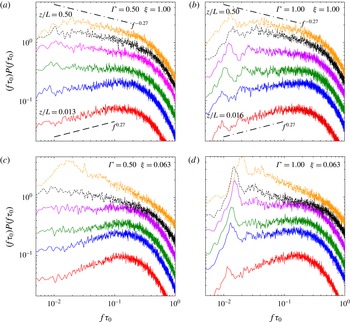
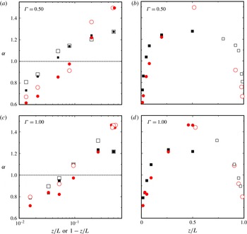
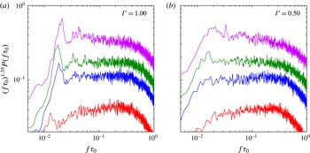
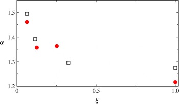
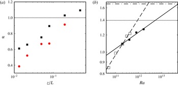
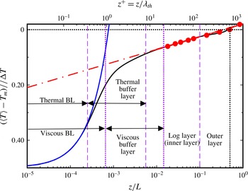
1 Introduction
Turbulent Rayleigh–Bénard convection (RBC) occurs in a fluid confined between parallel horizontal plates heated from below – for a general introduction, see e.g. Kadanoff (Reference Kadanoff2001) or Ahlers (Reference Ahlers2009); for more detailed reviews, see e.g. Ahlers, Grossmann & Lohse (Reference Ahlers, Grossmann and Lohse2009), Lohse & Xia (Reference Lohse and Xia2010) and Chillà & Schumacher (Reference Chillà and Schumacher2012). In this system, most of the temperature drop
 $\unicode[STIX]{x0394}T=T_{b}-T_{t}$
across the sample is sustained by two thin thermal boundary layers (BLs), one below the top plate at temperature
 $T_{t}$
and the other above the bottom plate at
 $T_{b}$
(Malkus Reference Malkus1954; Priestley Reference Priestley1954, Reference Priestley1959; Spiegel Reference Spiegel1971). The temperature in the bulk of the sample is fluctuating vigorously, but its time average varies only slowly with vertical position (Tilgner, Belmonte & Libchaber Reference Tilgner, Belmonte and Libchaber1993; Lui & Xia Reference Lui and Xia1998; Wang & Xia Reference Wang and Xia2003; Brown & Ahlers Reference Brown and Ahlers2007b
; Ahlers et al.
Reference Ahlers, Bodenschatz, Funfschilling, Grossmann, He, Lohse, Stevens and Verzicco2012; Ahlers, Bodenschatz & He Reference Ahlers, Bodenschatz and He2014; Wei & Ahlers Reference Wei and Ahlers2014) and is close to the mean temperature
 $T_{m}=(T_{b}+T_{t})/2$
.
Turbulent RBC is often studied using cylindrical samples with aspect ratio
 $\unicode[STIX]{x1D6E4}$
(diameter
 $D$
over height
 $L$
) close to one. In such systems, there is a large-scale circulation (LSC) in the sample interior (see e.g. Sano, Wu & Libchaber Reference Sano, Wu and Libchaber1989; Verzicco & Camussi Reference Verzicco and Camussi1999; Qiu & Tong Reference Qiu and Tong2001; Qiu et al.
Reference Qiu, Shang, Tong and Xia2004; Sun, Xia & Tong Reference Sun, Xia and Tong2005b
) that takes the form of a single convection roll with a circulation-plane orientation
 $\unicode[STIX]{x1D703}_{0}$
that is diffusing azimuthally and an amplitude
 $\unicode[STIX]{x1D6FF}$
that is varying stochastically under the influence of the velocity fluctuations (Brown, Nikolaenko & Ahlers Reference Brown, Nikolaenko and Ahlers2005; Sun, Xi & Xia Reference Sun, Xi and Xia2005a
; Brown & Ahlers Reference Brown and Ahlers2006b
, Reference Brown and Ahlers2008b
; He, Bodenschatz & Ahlers Reference He, Bodenschatz and Ahlers2016b
). The LSC carries plumes of hot or cold fluid emitted from the BLs, and in turn is driven by the buoyancy provided by these plumes.
Recently it was found (He et al.
Reference He, van Gils, Bodenschatz and Ahlers2014) for a sample with Prandtl number (see (3.2))
 $Pr\simeq 0.8$
that the temperature variance
 $\unicode[STIX]{x1D70E}^{2}$
(see (3.6)) varies logarithmically with the distance
 $z$
from the bottom or
 $1-z$
from the top plate throughout ‘inner layers’ which are outside the boundary layers and extend from approximately 1 % to 10 % or so of the bulk of the sample from each plate. This finding has analogues in wall-bounded turbulent shear flow, where the variance
 $\unicode[STIX]{x1D70E}_{v}^{2}$
of the downstream velocity was found to have a spatial range in which it depends logarithmically on the distance from the wall (Hultmark et al.
Reference Hultmark, Vallikivi, Bailey and Smits2012; Rosenberg et al.
Reference Rosenberg, Hultmark, Vallikivi, Bailey and Smits2013). In this inner layer of RBC, the normalized temperature power spectra
 $P(f\unicode[STIX]{x1D70F}_{0})$
were found to have a range of frequency
 $f$
covering a decade or more, where
 $$\begin{eqnarray}P(f\unicode[STIX]{x1D70F}_{0})=P_{0}(f\unicode[STIX]{x1D70F}_{0})^{-\unicode[STIX]{x1D6FC}},\end{eqnarray}$$
with
 $\unicode[STIX]{x1D6FC}\simeq 1.0$
. Here
 $\unicode[STIX]{x1D70F}_{0}$
is a characteristic time scale defined by (5.2) below and
 $P_{0}=0.208$
was found to be a constant independent of the axial and radial locations
 $z$
and
 $r$
, and the Rayleigh number
 $Ra$
(see (3.1)). As will be discussed below in § 6, these results for
 $\unicode[STIX]{x1D70E}^{2}$
and
 $P(f\unicode[STIX]{x1D70F}_{0})$
of the temperature field in RBC are consistent with a theoretical model by Townsend (Reference Townsend1976) and Perry, Henbest & Chong (Reference Perry, Henbest and Chong1986) for the velocity field in wall-bounded shear flow (the Townsend–Perry (TP) model), and an analogous model can be developed for RBC when it is assumed that the plumes take the place of the coherent eddies of the TP model (He, Bodenschatz & Ahlers Reference He, Bodenschatz and Ahlers2016a
).
In this paper we present local temperature measurements for two samples, one with aspect ratio (see (3.3))
 $\unicode[STIX]{x1D6E4}=0.50$
and the other with
 $\unicode[STIX]{x1D6E4}=1.00$
, with a larger
 $Pr=12.3$
, and find a very different result for
 $\unicode[STIX]{x1D70E}^{2}(z,r)$
and
 $P(f\unicode[STIX]{x1D70F}_{0})$
. The power law
 $$\begin{eqnarray}\unicode[STIX]{x1D70E}^{2}(\unicode[STIX]{x1D709},z/L)=\unicode[STIX]{x1D70E}_{0}^{2}(z/L)^{-\unicode[STIX]{x1D701}(\unicode[STIX]{x1D709})}\end{eqnarray}$$
(where
 $\unicode[STIX]{x1D709}$
is the dimensionless distance from the sidewall, see (3.5)) provides an excellent fit to results for the variance
 $\unicode[STIX]{x1D70E}^{2}$
of the temperature fluctuations, while a fit of the logarithmic dependence
 $$\begin{eqnarray}\unicode[STIX]{x1D70E}^{2}(\unicode[STIX]{x1D709},z/L)=M(\unicode[STIX]{x1D709})\ln (z/L)+N(\unicode[STIX]{x1D709})\end{eqnarray}$$
to the data is not as good. For both
 $\unicode[STIX]{x1D6E4}$
, we found
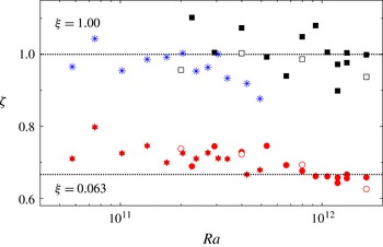
 $\unicode[STIX]{x1D701}\simeq 0.7$
close to the sample sidewall where most of the plumes are rising or falling and where temperature variations due to the stochastic LSC dynamics are largest, and
 $\unicode[STIX]{x1D701}\simeq 1.0$
close to the vertical sample centreline where LSC activity is minimal and plumes are found mostly near the plates where they travel roughly horizontally with the LSC. At a given radial location,
 $\unicode[STIX]{x1D701}$
is, within our resolution, independent of
 $Ra$
. For the spectra we again find a significant frequency range where
 $P(f\unicode[STIX]{x1D70F}_{0})\sim (f\unicode[STIX]{x1D70F}_{0})^{-\unicode[STIX]{x1D6FC}}$
, but
 $\unicode[STIX]{x1D6FC}$
varies from approximately
 $0.74$
near the top or bottom plate to approximately
 $1.27$
near the sample centre. These results do not agree with the TP model. While the data for
 $\unicode[STIX]{x1D70E}^{2}$
at a particular radial location may be consistent with one or the other of the models for RBC due to Priestley (Reference Priestley1954), Castaing et al. (Reference Castaing, Gunaratne, Heslot, Kadanoff, Libchaber, Thomae, Wu, Zaleski and Zanetti1989), Chung, Yun & Adrian (Reference Chung, Yun and Adrian1992) and Adrian (Reference Adrian1996) (see § 6), no one model explains their radial dependence. As discussed in § 2, there are good reasons to doubt that any model proposed so far is adequate to fully capture the composite nature, with multiple contributions, of fluctuations in RBC.
In the next section we discuss the several contributions to temperature fluctuations in RBC. These include contributions from the background turbulent fluctuations, from hot or cold plumes passing by the observation point, from the stochastic dynamics of the LSC, and from the torsional and sloshing mode of the LSC. To our knowledge, the LSC contributions to temperature fluctuations in RBC has not been considered quantitatively before. Then, in § 3, we define the parameters and symbols used in this paper. In § 4, we describe briefly the apparatus and the method of data acquisition and analysis. The results of our experiments are given in § 5. There, in § 5.1, we present measurements of the LSC temperature amplitude
 $\unicode[STIX]{x1D6FF}$
and of the orientation
 $\unicode[STIX]{x1D703}_{0}$
of the LSC circulation plane, and make an estimate of the LSC contribution to fluctuations in the horizontal midplane near the wall where
 $\unicode[STIX]{x1D6FF}$
and
 $\unicode[STIX]{x1D703}_{0}$
are measured. Then, in the remainder of § 5, we present evidence for a spatially uniform fluctuating mode (§ 5.2), and report on measurements of the characteristic time
 $\unicode[STIX]{x1D70F}_{0}$
(§ 5.3), of the temperature probability distribution skewness
 $S$
and kurtosis
 $K$
(§ 5.4), of the temperature variance
 $\unicode[STIX]{x1D70E}^{2}$
(§ 5.5), and of the temperature power spectra
 $P(f\unicode[STIX]{x1D70F}_{0})$
(§ 5.6). In § 6 we first give a brief historical review of fluctuation studies in RBC. Then we mention the models that have been proposed for
 $\unicode[STIX]{x1D70E}^{2}(z)$
and
 $P(f\unicode[STIX]{x1D70F}_{0})$
even though none of them may be adequate to deal with the complexities introduced by the LSC dynamics, and discuss some results of previous measurements. We conclude the paper with a summary of our findings (§ 7).
2 On the nature of fluctuations in turbulent convection
While we believe that the statistical properties of the temperature fluctuations in RBC such as
 $\unicode[STIX]{x1D70E}^{2}$
and
 $P(f\unicode[STIX]{x1D70F}_{0})$
are of interest and worth studying experimentally regardless of their origin, it is important for their ultimate theoretical understanding to appreciate that one can distinguish several contributions to these fluctuations. It was emphasized already by Grossmann & Lohse (Reference Grossmann and Lohse2004) that there is one contribution over a wide range of length and time scales from the turbulent background and another from the plumes that are emitted by the boundary layers and travel through the sample with the LSC. We shall refer to the sum of these as ‘intrinsic’ fluctuations. Here it is worth noting that only the sample centre at
 $\unicode[STIX]{x1D709}=1.00$
,
 $z/L=0.50$
is expected to be nearly free of the influence of plumes, and thus perhaps capable of revealing the genuine nature of the background fluctuations of the turbulent flow.
There are, however, further contributions which come from the LSC. The LSC occurs on a length scale that is of the order of the sample size. It is the source of the mean-flow velocity of the system, and by itself it would not contribute to fluctuations. However, the LSC is driven stochastically by the smaller-scale intrinsic fluctuations and thus has its own stochastic dynamics (Brown & Ahlers Reference Brown and Ahlers2007a , Reference Brown and Ahlers2008b ), which will also contribute to the locally measured fluctuations. This contribution has two parts. One part contributes at or near a characteristic frequency and is due to the sloshing and torsional modes of the LSC. The other is a broad-band contribution due to the stochastic variation of the LSC amplitude and orientation. It is difficult to accurately separate the intrinsic and LSC contributions, and in the present paper we shall not attempt to do so systematically. However, below in § 5.1 we shall make some estimates of the relative sizes of these contributions near the horizontal midplane of the sample. Again, we do not expect the LSC dynamics to have a significant influence at the sample centre, except perhaps for a contribution at a characteristic frequency of the sloshing mode, which can be removed in frequency space.
For a sample with
 $\unicode[STIX]{x1D6E4}\gg 1$
, one should expect the problem to become more complex because it is expected that the LSC will consist of many convection cells that will diffuse laterally, with individual cells growing and decaying at irregular time intervals in a random manner under the influence of the small-scale intrinsic fluctuations. An initial step towards investigating this large-scale dynamics was undertaken by direct numerical simulation (DNS) at relatively small
 $Ra$
(Bailon-Cuba, Emran & Schumacher Reference Bailon-Cuba, Emran and Schumacher2010), but to our knowledge there are no quantitative numerical studies, e.g. of spectra, variances and so forth, especially at larger
 $Ra$
. Experimental investigations also have only just begun (Hogg & Ahlers Reference Hogg and Ahlers2013), on a sample with
 $\unicode[STIX]{x1D6E4}=10.9$
. A consequence of the lateral diffusion of the LSC cells at sufficiently large
 $\unicode[STIX]{x1D6E4}$
is that the mean-flow velocity
 $U$
and the associated Reynolds number
 $Re_{U}$
vanish in the time average when measured at a fixed location within the sample. Indeed, it was found experimentally that
 $Re_{U}$
is two orders of magnitude smaller than the fluctuation Reynolds number
 $Re_{V}$
(based on the root-mean-square velocity
 $V$
) for a sample with
 $\unicode[STIX]{x1D6E4}=10.9$
(Hogg & Ahlers Reference Hogg and Ahlers2013). Interestingly, the lateral diffusion of the LSC cells, while it causes
 $Re_{U}$
to average to zero, contributes importantly to the measured values of
 $Re_{V}$
,
 $\unicode[STIX]{x1D70E}^{2}$
and
 $P(f\unicode[STIX]{x1D70F}_{0})$
.
In view of the fact that
 $\unicode[STIX]{x1D70E}^{2}$
and
 $P(f\unicode[STIX]{x1D70F}_{0})$
are hybrid quantities with multiple contributions, care must be exercised in comparing the measurements with any theoretical models, which may include only one or the other of these contributions but probably not all.
3 Relevant parameters
Experiments on thermal convection often are done in cylindrical vessels of diameter
 $D$
and height
 $L$
confined by a warm plate of temperature
 $T_{b}$
from below and a colder plate at temperature
 $T_{t}$
from above. If the temperature difference
 $\unicode[STIX]{x0394}T=T_{b}-T_{t}$
is sufficiently small, fluid properties can be assumed to be constant throughout the cell and the system is described by the Oberbeck–Boussinesq equations (Oberbeck Reference Oberbeck1879; Boussinesq Reference Boussinesq1903). Then there are two dimensionless control parameters, namely the Rayleigh number
 $$\begin{eqnarray}Ra=\frac{\unicode[STIX]{x1D6FC}_{P}g\unicode[STIX]{x0394}TL^{3}}{\unicode[STIX]{x1D708}\unicode[STIX]{x1D705}}\end{eqnarray}$$
and the Prandtl number
 $$\begin{eqnarray}Pr=\frac{\unicode[STIX]{x1D708}}{\unicode[STIX]{x1D705}}.\end{eqnarray}$$
Here
 $\unicode[STIX]{x1D6FC}_{P}$
,
 $\unicode[STIX]{x1D705}$
and
 $\unicode[STIX]{x1D708}$
denote the isobaric thermal expansion coefficient, the thermal diffusivity and the kinematic viscosity of the fluid. These properties are evaluated at the mean temperature
 $T_{m}=(T_{b}+T_{t})/2$
. The gravitational acceleration is
 $g$
. For a cylindrical sample, a third relevant parameter is the aspect ratio
 $$\begin{eqnarray}\unicode[STIX]{x1D6E4}\equiv D/L.\end{eqnarray}$$
An important global property usually investigated is the heat flux from the bottom to the top plate as expressed by the dimensionless Nusselt number
 $$\begin{eqnarray}Nu=\frac{QL}{A\unicode[STIX]{x1D706}\unicode[STIX]{x0394}T}.\end{eqnarray}$$
This quantity compares the overall heat current density
 $Q/A$
to the purely conductive heat flux
 $\unicode[STIX]{x1D706}\unicode[STIX]{x0394}T/L$
that would occur without convection.
We shall use
 $z$
for the vertical coordinate and set
 $z=0$
at the bottom plate. Often it will be convenient to use the dimensionless vertical coordinate
 $z/L$
. For the radial coordinate
 $r$
we shall use the dimensionless form
 $$\begin{eqnarray}\unicode[STIX]{x1D709}=1-r/R,\end{eqnarray}$$
where
 $R=D/2$
is the sample radius. Thus
 $\unicode[STIX]{x1D709}=0$
at the sidewall, and
 $\unicode[STIX]{x1D709}=1$
at the vertical sample centreline.
Local measurements of
 $T(t,z,r)$
(where
 $t$
is the time) were used to compute the normalized temperature probability distribution, and its variance
 $$\begin{eqnarray}\unicode[STIX]{x1D70E}^{2}(z,r)\equiv \langle [T(t,z,r)-\langle T(t,z,r)\rangle ]^{2}\rangle ,\end{eqnarray}$$
skewness
 $$\begin{eqnarray}m_{3}\equiv \langle [T(t,z,r)-\langle T(t,z,r)\rangle ]^{3}\rangle ,\end{eqnarray}$$
scaled skewness
 $$\begin{eqnarray}S=m_{3}/\unicode[STIX]{x1D70E}^{3/2},\end{eqnarray}$$
kurtosis
 $$\begin{eqnarray}m_{4}\equiv \langle [T(t,z,r)-\langle T(t,z,r)\rangle ]^{4}\rangle ,\end{eqnarray}$$
scaled kurtosis
 $$\begin{eqnarray}K=m_{4}/\unicode[STIX]{x1D70E}^{2},\end{eqnarray}$$
and the power spectra
 $\tilde{P}(f,z,r)$
of
 $T(t,z,r)-\langle T(t,z,r)\rangle _{t}$
. Here
 $\langle \cdots \rangle$
indicates the time average. We shall designate the normalized spectra by
 $P(f,z,r)=\tilde{P}(f,z,r)/\unicode[STIX]{x1D70E}^{2}(z,r)$
. We also computed correlation functions
 $$\begin{eqnarray}C_{T_{i},T_{j}}(\unicode[STIX]{x1D70F},z,r)=\frac{\langle \unicode[STIX]{x1D6FF}T_{j}(t+\unicode[STIX]{x1D70F},z,r)\,\unicode[STIX]{x1D6FF}T_{i}(t,z,r)\rangle }{\unicode[STIX]{x1D70E}_{i}(z,r)\unicode[STIX]{x1D70E}_{j}(z,r)}\end{eqnarray}$$
from temperature time sequences
 $T_{i}(t)$
and
 $T_{j}(t)$
with variances
 $\unicode[STIX]{x1D70E}_{i}^{2}$
and
 $\unicode[STIX]{x1D70E}_{j}^{2}$
.
4 Experimental set-up and data analysis
4.1 The experiment
The experiments were done using an apparatus described by Zhong & Ahlers (Reference Zhong and Ahlers2010) and Weiss & Ahlers (Reference Weiss and Ahlers2011c
). The versions used here were the
 $\unicode[STIX]{x1D6E4}=0.50$
sample described in detail by Wei & Ahlers (Reference Wei and Ahlers2014), and a new sample with
 $\unicode[STIX]{x1D6E4}=1.00$
. The
 $\unicode[STIX]{x1D6E4}=0.50$
cell had a cylindrical Lexan sidewall of inner diameter
 $D=19.0~\text{cm}$
and height
 $L=2.00D$
, while the
 $\unicode[STIX]{x1D6E4}=1.00$
sample had a Plexiglas sidewall with
 $L=D=24.1~\text{cm}$
. The thickness of both sidewalls was 0.63 cm. The fluid was the 3M fluorocarbon Fluorinert
 $^{\text{TM}}$
FC72 (perfluorohexane
 $\text{C}_{6}\text{F}_{14}$
; see also Wei & Ahlers (Reference Wei and Ahlers2014)) with
 $Pr=12.3$
. The mean temperature was
 $T_{m}=25.00\,^{\circ }\text{C}$
. FC72 has properties that permit access to exceptionally large values of
 $Ra$
for a given
 $L$
, but
 $L$
and
 $D$
are limited by the high cost of this fluid. The property values relevant to the present paper and at
 $25\,^{\circ }\text{C}$
are
 $\unicode[STIX]{x1D6FC}_{P}=1.60\times 10^{-3}~\text{K}^{-1}$
,
 $\unicode[STIX]{x1D705}=3.24\times 10^{-4}~\text{cm}^{2}~\text{s}^{-1}$
and
 $\unicode[STIX]{x1D708}=4.00\times 10^{-3}~\text{cm}^{2}~\text{s}^{-1}$
. The
 $Ra$
range extended from
 $5\times 10^{10}$
(for
 $\unicode[STIX]{x1D6E4}=1.00$
) to
 $2\times 10^{12}$
(for
 $\unicode[STIX]{x1D6E4}=0.50$
), corresponding to values of
 $\unicode[STIX]{x0394}T$
from 3 to 25 K for both
 $\unicode[STIX]{x1D6E4}$
. The top and bottom plates were made of copper.
Honeywell model 111-104HAK-H01 thermistors were inserted directly into the fluid for the temperature measurements. Their performance was discussed in the supplement to He et al. (Reference He, van Gils, Bodenschatz and Ahlers2014), where they are identified as
 $T_{2}$
. For both samples they were arranged in several vertical columns labelled
 $V_{i,j}$
, where
 $i$
and
 $j$
identify the radial and vertical positions, respectively. Details of the thermometer positions for the
 $\unicode[STIX]{x1D6E4}=0.50$
sample were given by Wei & Ahlers (Reference Wei and Ahlers2014). For the present work we used only
 $V_{0}$
and
 $V_{1}$
located for both samples at
 $\unicode[STIX]{x1D709}=1.00$
and
 $0.063$
, respectively, and some additional thermometers from
 $V_{2}$
and
 $V_{3}$
in or very near the horizontal midplane.
Statistical properties of the LSC were measured using the technique introduced by Brown et al. (Reference Brown, Nikolaenko and Ahlers2005) – see Brown & Ahlers (Reference Brown and Ahlers2006b
) and Funfschilling, Brown & Ahlers (Reference Funfschilling, Brown and Ahlers2008) for details; a related, albeit somewhat different, method had been used already by Cioni, Ciliberto & Sommeria (Reference Cioni, Ciliberto and Sommeria1997). For the
 $\unicode[STIX]{x1D6E4}=0.50$
sample, three sets of eight thermistors each (of the same type as above), azimuthally equally spaced, protruded through the sidewall to a radial position
 $\unicode[STIX]{x1D709}=0.063$
, one set each at three vertical positions. For
 $\unicode[STIX]{x1D6E4}=1.00$
there was only one set of eight thermistors, at
 $k=m$
. In that case the thermistors were embedded in blind holes in the sidewall. Thus their thermal response time was longer and they were not suitable for studying fluctuations, but we believe that they gave reliable measurements of time-averaged temperatures and LSC temperature amplitudes
 $\langle \unicode[STIX]{x1D6FF}_{m}\rangle$
(4.1).
The function
 $$\begin{eqnarray}T_{f,k}(t)=T_{w,k}(t)+\unicode[STIX]{x1D6FF}_{k}(t)\cos (\text{i}\unicode[STIX]{x03C0}/4-\unicode[STIX]{x1D703}_{0,k}(t))\end{eqnarray}$$
was fitted to the temperature readings
 $T_{k,i}(t)$
,
 $i=0,\ldots ,7$
, in a given horizontal plane and at each time
 $t$
by least-squares adjusting
 $T_{w,k}(t)$
,
 $\unicode[STIX]{x1D6FF}_{k}(t)$
and
 $\unicode[STIX]{x1D703}_{0,k}(t)$
. Here
 $k$
is an index indicating the vertical location at
 $z/L=0.25$
(
 $k=b$
),
 $z/L=0.50$
(
 $k=m$
) and
 $z/L=0.75$
(
 $k=t$
).
We also computed the coefficients of the lowest Fourier modes of the azimuthal temperature variation from the temperatures
 $T_{k,i}$
at a given
 $k$
(after having subtracted their mean
 $T_{w,k}$
) (Kunnen, Clercx & Geurts Reference Kunnen, Clercx and Geurts2008; Stevens, Clercx & Lohse Reference Stevens, Clercx and Lohse2011; Weiss & Ahlers Reference Weiss and Ahlers2011a
). This yielded the Fourier coefficients
 $A_{k,j}$
(the cosine coefficients) and
 $B_{k,j}$
(the sine coefficients) where
 $j=1,\ldots ,4$
identifies the four Fourier modes accessible with eight thermometers. From these coefficients we determined the ‘energy’
 $$\begin{eqnarray}E_{k,j}(t)=A_{k,j}^{2}(t)+B_{k,j}^{2}(t)\end{eqnarray}$$
for each mode, as well as the sum
 $E_{k,tot}(t)$
of these energies. Here we report the ratios of the time averages
 $$\begin{eqnarray}E_{k,1}/E_{k,tot}=\langle E_{k,1}(t)\rangle /\langle E_{k,tot}(t)\rangle .\end{eqnarray}$$
A closely related quantity suggested elsewhere (Stevens et al. Reference Stevens, Clercx and Lohse2011) is the parameter
 $$\begin{eqnarray}S_{k}=(NE_{k,1}/E_{k,tot}-1)/(N-1),\end{eqnarray}$$
where
 $N=4$
is the number of resolved Fourier modes in the plane at level
 $k$
.
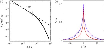
(a) Power spectrum of the temperature fluctuations at the sample centre (
 $\unicode[STIX]{x1D6E4}=0.50$
,
 $\unicode[STIX]{x1D709}=1.00$
,
 $z/L=0.50$
) for
 $Ra=1.67\times 10^{12}$
(
 $\unicode[STIX]{x0394}T=25.0~\text{K}$
). The vertical dotted lines indicate the frequency range used in the power-law fit. The dashed line is the result of that fit. (b) Autocorrelation functions for
 $\unicode[STIX]{x1D6E4}=0.50$
,
 $Ra=1.67\times 10^{12}$
and
 $\unicode[STIX]{x1D709}=0.063$
, at vertical positions
 $z/L=0.022$
(solid red), 0.080 (dotted purple) and 0.200 (dashed blue lines).

4.2 Data acquisition and analysis
‘Slow’ time sequences were taken using a single Agilent model 3497A Data Acquisition/Switch Unit with multiplexers. For the
 $\unicode[STIX]{x1D6E4}=1.00$
(
 $\unicode[STIX]{x1D6E4}=0.50$
) sample, we recorded 55 (79) temperatures simultaneously at time intervals of 5.2 (5.9) s. These sequences usually were quite long, spanning a day or more, and provided good statistics in cases where high time resolution was not required.
‘Fast’ time sequences of thermistor resistances were taken using a separate Agilent model 3497A Data Acquisition/Switch Unit for each thermistor. This allowed sampling of 50 000 data points at a rate of approximately 16 Hz, covering a time interval of approximately 50 min, while the resistances and time stamps were stored in the multimeter. Up to 20 such sequences, taken after all transients had decayed, were measured in a given run. Each sequence was analysed separately, and the resulting variances, power spectra and correlation functions were then averaged.
Figure 1(a) shows a typical averaged power spectrum based on fast sequences for
 $\unicode[STIX]{x1D6E4}=0.50$
. It was taken at the sample centre, for
 $Ra=1.67\times 10^{12}$
. One sees that the Nyquist frequency of 8 Hz is just high enough for the power to have decayed to the experimental noise level. The power spans just over five decades, and any power above the Nyquist frequency is too small to significantly contaminate the results over the frequency range of interest. Over a range of about a decade, the power can be described well by a power law. A fit over the range from 0.05 to 0.5 Hz (indicated by the two vertical dotted lines) yielded the power-law exponent
 $\unicode[STIX]{x1D6FC}=1.27\pm 0.01$
. Similar analyses yielded the results for
 $\unicode[STIX]{x1D6FC}$
discussed below.
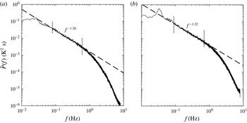
Power spectra of the temperature fluctuations for
 $\unicode[STIX]{x1D6E4}=1.00$
and
 $Ra=0.40\times 10^{12}$
(
 $\unicode[STIX]{x0394}T=25~\text{K}$
). (a) The spectrum at the sample centre (
 $\unicode[STIX]{x1D709}=1.00$
,
 $z/L=0.50$
). (b) The spectrum closer to the sidewall (
 $\unicode[STIX]{x1D709}=0.063$
,
 $z/L=0.26$
). The vertical dotted lines indicate the frequency ranges used in the power-law fits. The dashed lines are the results of those fits.

Figure 2 presents two spectra for
 $\unicode[STIX]{x1D6E4}=1.00$
. The measurements were made with the same
 $\unicode[STIX]{x0394}T=25.0~\text{K}$
that was used to obtain the data in figure 1(a), but, in view of the smaller sample height, the Rayleigh number
 $Ra=0.40\times 10^{12}$
was smaller. The spectrum in figure 2(a) was measured at the sample centre. It does not differ much from the one at the same location but for
 $\unicode[STIX]{x1D6E4}=0.50$
(figure 1
a), except for a barely noticeable peak near
 $f=0.025$
Hz, which we attribute to the sloshing mode of the LSC (Brown & Ahlers Reference Brown and Ahlers2009; Xi et al.
Reference Xi, Zhou, Zhou, Chan and Xia2009; Zhou et al.
Reference Zhou, Xi, Zhou, Sun and Xia2009). This mode, as well as the torsional mode (Funfschilling & Ahlers Reference Funfschilling and Ahlers2004; Funfschilling et al.
Reference Funfschilling, Brown and Ahlers2008), is not well developed or is absent for
 $\unicode[STIX]{x1D6E4}=0.50$
and thus in that case does not contribute noticeably to the spectra. A fit of a power law over the range from 0.08 to 0.6 Hz yielded the exponent
 $\unicode[STIX]{x1D6FC}=1.26\pm 0.01$
, the same within the uncertainty as for
 $\unicode[STIX]{x1D6E4}=0.50$
(see, however, § 5.6 and figure 21(b) below).
The spectrum in figure 2(b) is for
 $\unicode[STIX]{x1D6E4}=1.00$
,
 $\unicode[STIX]{x1D709}=0.063$
and
 $z/L=0.26$
. There is a much larger peak near 0.03 Hz due to the torsional mode of the LSC, which for the case shown we estimate to contribute 12 % to the total power. Just above it a much smaller contribution from a second harmonic is observable as well. In view of these contributions, measurements of the variance
 $\unicode[STIX]{x1D70E}^{2}$
(the integral of the power spectrum), the skewness
 $m_{3}$
and the kurtosis
 $m_{4}$
will contain an LSC contribution and are not reliable measures of the contribution from the local intrinsic temperature fluctuations alone. There is, however, a decade of
 $f$
above these peaks over which
 $P(f)$
follows a power law, and an exponent
 $\unicode[STIX]{x1D6FC}$
unencumbered by the sloshing and torsional modes can still be determined from the spectra. However, as we shall discuss below in § 5.1, the stochastic dynamics of the LSC (Brown & Ahlers Reference Brown and Ahlers2006b
, Reference Brown and Ahlers2008b
) contributes broadly and significantly to the spectrum, and thus will influence
 $\unicode[STIX]{x1D70E}^{2}$
,
 $m_{3}$
and
 $m_{4}$
, and potentially it can affect
 $\unicode[STIX]{x1D6FC}$
as well. The particular example in figure 2(b) yields
 $\unicode[STIX]{x1D6FC}=1.22\pm 0.01$
from the data between the dotted vertical lines at 0.09 and 0.7 Hz. We expect that the LSC dynamics does not contribute significantly at the sample centre where the local time-averaged velocity of the LSC is expected to vanish (Qiu & Tong Reference Qiu and Tong2000, Reference Qiu and Tong2001).
Figure 1(b) shows examples of autocorrelation functions
 $C(\unicode[STIX]{x1D70F},z,r)$
for
 $\unicode[STIX]{x1D6E4}=0.50$
. These results are for
 $Ra=1.67\times 10^{12}$
at the radial position
 $\unicode[STIX]{x1D709}=0.063$
, and for three different vertical positions. One sees that the correlation functions decay to zero, as they should for a statistically stationary process (there are no significant oscillations or deviations from zero at times larger than 30 s). Results for
 $\unicode[STIX]{x1D6E4}=1.00$
are similar and will not be shown.
To obtain the fluctuations of the LSC temperature amplitudes
 $\unicode[STIX]{x1D6FF}_{k}$
and orientations
 $\unicode[STIX]{x1D703}_{k}$
(see (4.1)), it was necessary to measure eight temperatures simultaneously and synchronously. This was accomplished by triggering eight separate multimeters virtually simultaneously. Each gave a member of a time sequence of the thermometer resistance and a corresponding time stamp. By interpolating in time for each sequence, we produced the needed virtually simultaneous sequences.
5 Results
5.1 The large-scale circulation
In this subsection we present results that establish the existence of an LSC in the form of a single convection roll in both of our samples, and show that the LSC dynamics contributes importantly to the variance of local temperature measurements at least near the sidewall.
5.1.1 Time-averaged large-scale circulation properties
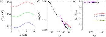
In figure 3(a) we show the time averages
 $\langle T_{k,i}\rangle$
of the near-sidewall temperature measurements at
 $\unicode[STIX]{x1D709}=0.063$
for
 $\unicode[STIX]{x1D6E4}=0.50$
as a function of azimuthal position. If the LSC circulation-plane orientation diffused randomly over all angles, this average would be independent of
 $\unicode[STIX]{x1D703}$
; but for a variety of reasons (Brown & Ahlers Reference Brown and Ahlers2006a
, Reference Brown and Ahlers2008a
; He et al.
Reference He, Bodenschatz and Ahlers2016b
) there always is a preferred orientation (see figure 5 below) and the LSC signature survives in
 $\langle T_{k,i}\rangle$
. One sees that the results at the three vertical positions are in phase, indicating the existence of an LSC that is vertically coherent in the time average. This finding is consistent with the results of Weiss & Ahlers (Reference Weiss and Ahlers2011c
) (see also Xi & Xia Reference Xi and Xia2008), who found for
 $\unicode[STIX]{x1D6E4}=0.50$
and
 $Pr=4.38$
that the LSC consists of a single convection roll when
 $Ra\gtrsim 10^{11}$
.
Properties of the large-scale circulation. (a) The time-averaged temperatures very near the sidewall (
 $\unicode[STIX]{x1D709}=0.063$
) for
 $\unicode[STIX]{x1D6E4}=0.50$
and
 $Ra=1.33\times 10^{12}$
(
 $\unicode[STIX]{x0394}T=20.0$
K). The data are for
 $z/L=0.25$
(red diamonds),
 $z/L=0.50$
(green circles) and
 $z/L=0.75$
(blue squares). The lines are fits of (4.1) to the time averages
 $\langle T_{k,i}\rangle$
of
 $T_{k,i}$
. (b) Time-averaged values
 $\langle \unicode[STIX]{x1D6FF}_{k}(t)\rangle$
of the LSC temperature amplitudes (see (4.1)). Solid symbols and star for
 $\unicode[STIX]{x1D6E4}=1.00$
: solid purple circles,
 $\langle \unicode[STIX]{x1D6FF}_{m}\rangle$
from the
 $\unicode[STIX]{x1D6E4}=1.00$
sample of Wei & Ahlers (Reference Wei and Ahlers2014); solid black squares,
 $\langle \unicode[STIX]{x1D6FF}_{m}\rangle$
from the
 $\unicode[STIX]{x1D6E4}=1.00$
sample described in the present paper; black stars,
 $\langle \unicode[STIX]{x1D6FF}_{m}(t)\rangle$
for
 $\unicode[STIX]{x1D6E4}=1.00$
for
 $Pr=4.38$
from Brown & Ahlers (Reference Brown and Ahlers2007b
). Open symbols for
 $\unicode[STIX]{x1D6E4}=0.50$
: red diamonds,
 $k=b~(z/L=0.25)$
; green circles,
 $k=m~(z/L=0.50)$
; blue squares,
 $k=t~(z/L=0.75)$
. (c) The ratio of the time average of the energy of the first Fourier mode to the time average of the total energy,
 $E_{k,1}/E_{k,tot}$
(4.3), as a function of
 $Ra$
. The symbols are as in (b), except that the green stars show the parameter
 $S_{m}$
(4.4) for
 $\unicode[STIX]{x1D6E4}=0.50$
.

The four mean values of the pairs of
 $\langle T_{m,i}\rangle$
with members displaced azimuthally by a distance of
 $\unicode[STIX]{x03C0}$
from each other were found to be in the range
 $25.199\,^{\circ }\text{C}\pm 0.001~\text{K}$
. The azimuthal mean
 $\bar{T}$
of all the temperatures
 $\langle T_{m,i}\rangle$
measured at
 $z/L=0.50$
(green circles) also was
 $\bar{T}=25.199\,^{\circ }$
C. These estimates agree well with the measured time-averaged temperature
 $T_{c}=25.196^{\circ }$
C at the sample centre. The results indicate that, as expected for a single-roll LSC, there is a spatially uniform time-averaged temperature
 $\bar{T}$
in the horizontal midplane. It differs slightly from the mean temperature
 $T_{m}=25.000^{\circ }$
C, with
 $(\bar{T}-T_{m})/\unicode[STIX]{x0394}T=0.010$
. The deviation of this value from zero is a measure of the influence of non-Boussinesq effects, which are seen to be quite small.
Figure 3(b) shows the time-averaged amplitudes
 $\langle \unicode[STIX]{x1D6FF}_{k}\rangle$
, scaled by the applied temperature difference
 $\unicode[STIX]{x0394}T$
, as a function of
 $Ra$
for several samples. The solid circles are for
 $Pr=12.3$
at
 $k=m$
from the
 $\unicode[STIX]{x1D6E4}=1.00$
sample used by Wei & Ahlers (Reference Wei and Ahlers2014), and the solid black squares were obtained from the
 $\unicode[STIX]{x1D6E4}=1.00$
sample at
 $k=m$
of this work. In the overlapping range of
 $Ra$
, the two datasets agree very well. For comparison we show also the
 $\unicode[STIX]{x1D6E4}=1.00$
data from Brown & Ahlers (Reference Brown and Ahlers2007b
) for
 $Pr=4.38$
(black stars). Although the Prandtl number is smaller, they do not differ much from the present results at the
 $Ra$
values where they nearly overlap. We note that all of these data were taken with thermistors embedded in the sidewalls.
The open symbols are for our
 $\unicode[STIX]{x1D6E4}=0.50$
sample, at the three vertical positions
 $z/L=0.25$
(red diamonds), 0.50 (green circles) and 0.75 (blue squares) measured with thermistors immersed in the fluid at
 $\unicode[STIX]{x1D709}=0.063$
. One sees that the amplitudes are slightly smaller (by approximately 15 % or so) at the midplane than they are at
 $z/L=0.25$
and 0.75. Similar results were found by Weiss & Ahlers (Reference Weiss and Ahlers2011c
, Reference Weiss and Ahlers2013) for
 $\unicode[STIX]{x1D6E4}=0.50$
and
 $Pr=4.38$
, but just the opposite was found by Brown & Ahlers (Reference Brown and Ahlers2007b
) for
 $\unicode[STIX]{x1D6E4}=1.00$
,
 $Pr=4.38$
and
 $Ra\lesssim 10^{10}$
. Relevant to our present work is the fact that, at the same
 $Ra$
and our
 $Pr=12.3$
, the LSC temperature amplitudes are not very different for the two aspect ratios. Thus, at the same
 $Ra$
, a single-roll LSC of similar strength exists (in the time average) for both
 $\unicode[STIX]{x1D6E4}$
values.
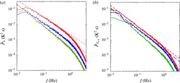
Power spectra for
 $\unicode[STIX]{x0394}T=25.0~\text{K}$
and
 $\unicode[STIX]{x1D6E4}=0.50$
(
 $Ra=1.67\times 10^{12}$
). (a) Spectra
 $\tilde{P}_{\unicode[STIX]{x1D6FF}}$
of
 $\unicode[STIX]{x1D6FF}_{k}$
. From bottom to top they are for
 $k=m$
(green),
 $k=t$
(blue) and
 $k=b$
(red). The power-law fits over one decade of
 $f$
(dashed lines) gave
 $\unicode[STIX]{x1D6FC}_{\unicode[STIX]{x1D6FF}_{m}}=1.42$
,
 $\unicode[STIX]{x1D6FC}_{\unicode[STIX]{x1D6FF}_{t}}=1.20$
and
 $\unicode[STIX]{x1D6FC}_{\unicode[STIX]{x1D6FF}_{b}}=1.13$
. (b) Spectra
 $\tilde{P}_{T_{w,k}}$
of
 $T_{w,k}$
to be discussed below in § 5.2. From bottom to top they are for
 $k=m$
(green),
 $k=t$
(blue) and
 $k=b$
(red). The power-law fits over one decade of
 $f$
(dashed lines) gave
 $\unicode[STIX]{x1D6FC}_{T_{w,m}}=1.521$
,
 $\unicode[STIX]{x1D6FC}_{T_{w,t}}=1.339$
and
 $\unicode[STIX]{x1D6FC}_{T_{w,b}}=1.334$
.

In figure 3(c) we show the ratio
 $E_{k,1}/E_{k,tot}$
of the time average of the energy of the first Fourier mode of the LSC temperature signature (equal to
 $\langle \unicode[STIX]{x1D6FF}_{k}^{2}\rangle$
) to the time average of the total energy (see (4.3)) as a function of
 $Ra$
. As noted before (Stevens et al.
Reference Stevens, Clercx and Lohse2011; Weiss & Ahlers Reference Weiss and Ahlers2011b
), for
 $\unicode[STIX]{x1D6E4}=1.00$
most of the energy is contained in the fundamental mode, which is attributed to the LSC, and only a small fraction is contained in higher modes, which are caused by smaller-scale fluctuations. For
 $\unicode[STIX]{x1D6E4}=0.50$
only about half the energy, roughly corresponding to
 $S_{k}=0.33$
(see (4.4)), is in the fundamental mode. This contribution is smaller than was found for
 $\unicode[STIX]{x1D6E4}=0.50$
,
 $Pr=4.38$
and
 $Ra=7\times 10^{10}$
, where Weiss & Ahlers (Reference Weiss and Ahlers2013) measured
 $E_{1}/E_{tot}=0.7$
. Part of this difference may be due to the fact that the earlier measurements were made with thermometers embedded in the sidewalls where fast fluctuations are attenuated, while the present results are from thermometers in the fluid. According to the criterion of Stevens et al. (Reference Stevens, Clercx and Lohse2011),
 $S_{k}\lesssim 0.5$
implies that the single-roll LSC is not dominant; but based on the compilation of data in figure 11 of Weiss & Ahlers (Reference Weiss and Ahlers2011c
), we expect the double-roll state to be essentially absent in our parameter range.
We were able to determine the LSC amplitudes
 $\unicode[STIX]{x1D6FF}_{k}$
and orientations
 $\unicode[STIX]{x1D703}_{0,k}$
quite unambiguously, with uncertainties much smaller than the values. In addition, the probability distributions of the orientations
 $\unicode[STIX]{x1D703}_{0,k}$
and the
 $\unicode[STIX]{x1D703}$
dependences of the time averages
 $\langle T_{k,i}\rangle$
(see figure 3
a) were very similar at the three levels
 $k=b,m,t$
. For these reasons, as well as because of the previous work compiled by Weiss & Ahlers (Reference Weiss and Ahlers2011c
), we believe that the LSC in the form of a single roll is present and that it has the potential to play a significant role in the generation of temperature fluctuations.
5.1.2 Large-scale circulation dynamics
As discussed in § 2, the LSC has a stochastic dynamics, driven by the smaller-scale fluctuations (Brown & Ahlers Reference Brown and Ahlers2006b
, Reference Brown and Ahlers2007a
, Reference Brown and Ahlers2008b
). Numerous previous publications reported that both the temperature amplitude
 $\unicode[STIX]{x1D6FF}_{k}(t)$
and the azimuthal orientation of the circulation plane
 $\unicode[STIX]{x1D703}_{0,k}(t)$
(see (4.1)) vary irregularly with the time
 $t$
. Here we report power spectra for
 $\unicode[STIX]{x1D6FF}_{k}$
at all three levels
 $k=b,m,t$
for
 $\unicode[STIX]{x1D6E4}=0.50$
. They are given in figure 4(a) (meaningful spectra for
 $\unicode[STIX]{x1D6E4}=1.00$
are not available because the thermometers were embedded in the sidewall and had long thermal time constants; thus they produced spectra that were heavily attenuated at large frequencies). As was the case for the individual temperatures, one sees that also the spectra of
 $\unicode[STIX]{x1D6FF}_{k}$
have a frequency range of about a decade over which they can be described by a power law analogous to (1.1) with exponents
 $\unicode[STIX]{x1D6FC}_{\unicode[STIX]{x1D6FF}_{m}}=1.42$
,
 $\unicode[STIX]{x1D6FC}_{\unicode[STIX]{x1D6FF}_{t}}=1.20$
and
 $\unicode[STIX]{x1D6FC}_{\unicode[STIX]{x1D6FF}_{b}}=1.13$
. One sees that the exponent is largest at the horizontal midplane
 $k=m$
, where it reaches a value of 1.42. We have no explanation for the small difference between
 $\unicode[STIX]{x1D6FC}_{\unicode[STIX]{x1D6FF}_{b}}$
and
 $\unicode[STIX]{x1D6FC}_{\unicode[STIX]{x1D6FF}_{t}}$
, which for a Boussinesq system should be equal to each other. Although measurements at many values of
 $Ra$
were not made, results obtained for
 $Ra=0.80\times 10^{12}$
gave
 $\unicode[STIX]{x1D6FC}_{\unicode[STIX]{x1D6FF}_{m}}=1.41$
and thus did not reveal a significant
 $Ra$
dependence.
The probability distribution
 $P(\unicode[STIX]{x1D703}_{0,m}/2\unicode[STIX]{x03C0})$
of the orientation of the LSC circulation plane as a function of
 $\unicode[STIX]{x1D703}/2\unicode[STIX]{x03C0}$
. (a) Plot for
 $\unicode[STIX]{x1D6E4}=1.00$
and
 $Ra=0.40\times 10^{12}$
. The dashed line is from figure 9 of Brown & Ahlers (Reference Brown and Ahlers2006a
) for
 $\unicode[STIX]{x1D6E4}=1.00$
,
 $Pr=4.38$
and
 $Ra=5\times 10^{9}$
. (b) Plot for
 $\unicode[STIX]{x1D6E4}=0.50$
and
 $Ra=1.67\times 10^{12}$
. The dashed line is from figure 16 of Weiss & Ahlers (Reference Weiss and Ahlers2011c
) for
 $\unicode[STIX]{x1D6E4}=0.50$
,
 $Pr=4.38$
and
 $Ra=9\times 10^{10}$
.

For an ideal rotationally invariant sample, one would expect a uniform probability distribution
 $P(\unicode[STIX]{x1D703}_{0,k})=1/(2\unicode[STIX]{x03C0})$
of the azimuthal orientation. In real experiments,
 $P(\unicode[STIX]{x1D703}_{0,k})$
is non-uniform due to several small perturbations (Brown & Ahlers Reference Brown and Ahlers2006a
, Reference Brown and Ahlers2008a
; Weiss & Ahlers Reference Weiss and Ahlers2011c
; He et al.
Reference He, Bodenschatz and Ahlers2016b
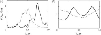
). In order to see whether any major non-uniformity was introduced by the thermometers that were inserted into the interior of our present samples, we show in figure 5 the distributions for (a)
 $\unicode[STIX]{x1D6E4}=1.00$
and (b)
 $\unicode[STIX]{x1D6E4}=0.50$
, together with previous measurements (dashed lines) for similar samples with no obstructions in their interiors. The relatively small difference in the widths of the distributions might be attributed to the intrusive thermometers; but it could also be caused by the large difference of
 $Pr$
and
 $Ra$
(the influence of which is unknown). The double-peaked structure in figure 5(b) (
 $\unicode[STIX]{x1D6E4}=0.50$
) most likely is caused by the thermometer column located at
 $\unicode[STIX]{x1D709}=1.00$
, the members of which were inserted into the sample at
 $\unicode[STIX]{x1D703}=0$
with their leads extending through thin ceramic tubes from the sidewall all the way to the sample centreline (see Wei & Ahlers Reference Wei and Ahlers2014). However, we have no evidence – and think it unlikely – that this perturbation will have a major effect on the other measured statistical properties.
In view of the stochastic dynamics of the LSC, the local temperature fluctuations induced by
 $\unicode[STIX]{x1D6FF}_{k}$
and
 $\unicode[STIX]{x1D703}_{0,k}$
, if they could be measured separately, would be stochastic as well and will contribute to
 $\unicode[STIX]{x1D70E}^{2}$
, to
 $P(f\unicode[STIX]{x1D70F}_{0})$
and to other statistical measures of the fluctuations. We shall designate this contribution to the variance as
 $\unicode[STIX]{x1D70E}_{LSC}^{2}$
. The size of
 $\unicode[STIX]{x1D70E}_{LSC}^{2}$
at
 $\unicode[STIX]{x1D709}=0.063$
can be estimated from a reconstruction of the temperature time series
 $$\begin{eqnarray}\unicode[STIX]{x1D6FF}T_{k}(t,\unicode[STIX]{x1D703})=\unicode[STIX]{x1D6FF}_{k}(t)\cos (\unicode[STIX]{x1D703}-\unicode[STIX]{x1D703}_{0,k}(t))\end{eqnarray}$$
from time series of
 $\unicode[STIX]{x1D6FF}_{k}(t)$
and
 $\unicode[STIX]{x1D703}_{0,k}(t)$
. When this is done,
 $\unicode[STIX]{x1D70E}_{LSC}^{2}$
is seen to make a significant, even dominant, contribution to
 $\unicode[STIX]{x1D70E}^{2}$
. In addition, we find that the temperatures
 $T_{w,k}(t)$
(see (4.1)) also vary irregularly in time, and we show their spectra in figure 4(b); but since they are azimuthally averaged quantities, we do not include them in any estimate of the LSC-induced fluctuations. We discuss
 $T_{w,m}(t)$
separately as a contribution to the intrinsic background fluctuations in § 5.2.
Solid line: the variance
 $\unicode[STIX]{x1D70E}_{LSC}^{2}/\unicode[STIX]{x0394}T^{2}$
of the temperature fluctuations induced by the stochastic LSC dynamics (see (5.1)) in the horizontal midplane at
 $\unicode[STIX]{x1D709}=0.063$
as a function of azimuthal position
 $\unicode[STIX]{x1D703}$
for
 $\unicode[STIX]{x1D6E4}=0.50$
and
 $Ra=1.67\times 10^{12}$
. Dashed line: the variance of
 $T_{w,m}$
under the same conditions. Black circles: the variance
 $\unicode[STIX]{x1D70E}^{2}/\unicode[STIX]{x0394}T^{2}$
measured directly with the thermometers in the horizontal midplane at
 $\unicode[STIX]{x1D709}=0.063$
that were used to determine the LSC amplitude and orientation using (4.1). Open square:
 $\unicode[STIX]{x1D70E}^{2}/\unicode[STIX]{x0394}T^{2}$
measured with the thermometer from the vertical column at
 $\unicode[STIX]{x1D709}=0.063$
and
 $z/L=0.50$
.

A detailed and quantitative study of
 $\unicode[STIX]{x1D70E}_{LSC}^{2}(z,r)$
will require faster sampling rates, simultaneously and synchronously at many locations, than we have available at present, as well as a model for the shape of the LSC. However, in order to illustrate semi-quantitatively the influence of the LSC dynamics on the measured temperature fluctuations, we reconstructed the time series, using (5.1), of the LSC-induced temperature fluctuations for
 $\unicode[STIX]{x1D6E4}=0.50$
and
 $Ra=1.67\times 10^{12}$
(
 $\unicode[STIX]{x0394}T=25.0~\text{K}$
) near the sidewall at
 $z/L=0.50$
(
 $k=m$
) and compared their variance with those of the directly measured fluctuations (based on (3.6)) at
 $\unicode[STIX]{x1D709}=0.063$
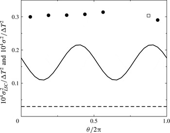
. Figure 6 shows
 $\unicode[STIX]{x1D70E}_{LSC}^{2}/\unicode[STIX]{x0394}T^{2}$
as a function of the azimuthal orientation
 $\unicode[STIX]{x1D703}/2\unicode[STIX]{x03C0}$
as a solid line. One sees that this variance depends on
 $\unicode[STIX]{x1D703}$
. We would have expected this not to be the case if
 $\unicode[STIX]{x1D703}_{0,m}$
had been uniformly distributed over all angles and uncorrelated with
 $\unicode[STIX]{x1D6FF}_{m}$
; but since
 $P(\unicode[STIX]{x1D703}_{0,m})$
depends on
 $\unicode[STIX]{x1D703}_{0,m}$
(see figure 5
b), the variance
 $\unicode[STIX]{x1D70E}_{LSC}^{2}$
does so as well. Indeed, as can be seen by comparing the two figures, the maxima of
 $\unicode[STIX]{x1D70E}_{LSC}^{2}(\unicode[STIX]{x1D703}_{0,m}/2\unicode[STIX]{x03C0})$
(figure 6) are located quite close to the maxima of
 $P(\unicode[STIX]{x1D703}_{0,m}/2\unicode[STIX]{x03C0})$
(figure 5
b).
Also shown, as solid circles, in figure 6 are measurements of
 $\unicode[STIX]{x1D70E}^{2}/\unicode[STIX]{x0394}T^{2}$
derived from (3.6) and based on the individual temperature measurements at
 $\unicode[STIX]{x1D709}=0.063$
, which were used to determine
 $\unicode[STIX]{x1D6FF}_{m}$
and
 $\unicode[STIX]{x1D703}_{0,m}$
from fits of (4.1). The result for
 $\unicode[STIX]{x1D70E}^{2}/\unicode[STIX]{x0394}T^{2}$
measured with the thermometer from the vertical column at
 $\unicode[STIX]{x1D709}=0.063$
and
 $z/L=0.50$
is represented by the open square. One sees that these data are only about a factor of 2 larger than
 $\unicode[STIX]{x1D70E}_{LSC}^{2}/\unicode[STIX]{x0394}T^{2}$
, thus showing that near the sidewall there is a major LSC contribution to the total variance of the temperature fluctuations. We would expect that
 $\unicode[STIX]{x1D70E}_{LSC}^{2}$
decreases as the radial position approaches the sample centreline, but there are no measurements to support this expectation.
For samples with
 $\unicode[STIX]{x1D6E4}$
close to one, the LSC makes yet another contribution
 $\unicode[STIX]{x1D70E}_{f}^{2}$
to
 $\unicode[STIX]{x1D70E}^{2}$
. It is localized in frequency and originates from a ‘torsional’ (Funfschilling & Ahlers Reference Funfschilling and Ahlers2004; Funfschilling et al.
Reference Funfschilling, Brown and Ahlers2008) and a ‘sloshing’ (Brown & Ahlers Reference Brown and Ahlers2009; Xi et al.
Reference Xi, Zhou, Zhou, Chan and Xia2009; Zhou et al.
Reference Zhou, Xi, Zhou, Sun and Xia2009) mode of the LSC, which typically are excited by the stochastic driving. This contribution, when present, contributes a somewhat broadened peak to
 $P(f\unicode[STIX]{x1D70F}_{0})$
(see figure 2
b). It can be separated in frequency space from the contributions due to the other fluctuations when it is assumed that the various terms are uncorrelated. In the particular example of figure 2(b), for instance, we estimate that it contributed 12 % to the total power
 $\unicode[STIX]{x1D70E}^{2}$
. For
 $\unicode[STIX]{x1D6E4}=0.50$
this mode is very weak or absent.
We note that the spectrum of
 $\unicode[STIX]{x1D6FF}T_{k}$
is broad and, unlike the contribution from the sloshing and torsional mode, cannot be separated in the frequency domain from that of the intrinsic contributions.
Finally, we note that the LSC contributions must be expected to be important as well in measurements of other properties such as the fluctuation Reynolds number
 $Re_{V}$
(see e.g. He et al.
Reference He, van Gils, Bodenschatz and Ahlers2015).
5.2 A spatially uniform fluctuating mode
One might have assumed that the azimuthally averaged temperatures
 $T_{w,k}$
(see (4.1)) would be essentially constant in time. This, however, is not the case. For
 $\unicode[STIX]{x1D6E4}=0.50$
and
 $Ra=1.67\times 10^{12}$
, we show their spectra in figure 4(b). The spectra also can be fitted with a power law over about a decade of
 $f$
, leading to the exponent values
 $\unicode[STIX]{x1D6FC}_{T_{w,m}}=1.521$
,
 $\unicode[STIX]{x1D6FC}_{T_{w,t}}=1.339$
and
 $\unicode[STIX]{x1D6FC}_{T_{w,b}}=1.334$
. Again, the exponent is largest at the horizontal midplane. For
 $Ra=0.80\times 10^{12}$
, we found
 $\unicode[STIX]{x1D6FC}_{T_{w,m}}=1.34$
, indicating an
 $Ra$
dependence of this exponent over our experimental range.
The above result implies that there is a large-scale mode that contributes uniformly at all azimuthal locations to the turbulent fluctuations. Its variance (the integral of
 $\tilde{P}_{T_{w,k}}$
) at
 $k=m$
, scaled by
 $\unicode[STIX]{x0394}T^{2}$
, is shown in figure 6 as a dashed line. Although its contribution is smaller than
 $\unicode[STIX]{x1D70E}_{LSC}^{2}$
, it is by no means negligible. Comparing with the solid circles in figure 6, one sees that its contribution to the total fluctuation power in the horizontal midplane near the sidewall is 5 % for that case.
(a) The cross-correlation function
 $C_{T_{c},T_{w,m}}$
between the sample centre temperature
 $T_{c}(t)$
and
 $T_{w,m}(t)$
(see (4.1)) for
 $\unicode[STIX]{x1D6E4}=0.50$
and
 $Ra=1.33\times 10^{12}$
(
 $\unicode[STIX]{x0394}T=20~\text{K}$
). The maximum
 $C_{0}$
, located at
 $\unicode[STIX]{x1D70F}=0$
, is indicated. (b) The maximum
 $C_{0}$
of
 $C_{T_{c},T_{w,m}}$
as a function of
 $Ra$
. (c) The cross-correlation function
 $C_{T_{w,m},\unicode[STIX]{x1D6FF}_{m}}$
between
 $T_{w,m}$
(see (4.1)) and the LSC temperature amplitude
 $\unicode[STIX]{x1D6FF}_{m}$
for
 $\unicode[STIX]{x1D6E4}=0.50$
at
 $Ra=1.33\times 10^{12}$
.

An interesting question is whether these azimuthally uniform fluctuations also extend radially into the sample interior. The time cross-correlation function between
 $T_{w,m}$
and the centre temperature
 $T_{c}$
at
 $Ra=1.33\times 10^{12}$
is shown as a function of the time delay
 $\unicode[STIX]{x1D70F}$
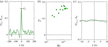
in figure 7(a). It is seen to have a sharp positive peak at
 $\unicode[STIX]{x1D70F}=0$
, indicating a significant correlation between the centre-temperature fluctuations and the fluctuations around the periphery. The height
 $C_{0}$
of this peak is shown as a function of
 $Ra$
in figure 7(b). The mode
 $T_{w,m}$
is uncorrelated with the LSC amplitude
 $\unicode[STIX]{x1D6FF}_{m}$
, as shown in figure 7(c).
5.3 The characteristic time scale
 $\unicode[STIX]{x1D70F}_{0}$

Previous suggestions have been made about how to scale the frequency of power spectra, with the aim of yielding an
 $Ra$
-independent curve at a given location within the sample, and especially at the sample centre. To that aim, Wu et al. (Reference Wu, Kadanoff, Libchaber and Sano1990) carried out an analysis based on a multifractal transformation involving adjustable parameters (see also Frisch Reference Frisch1995). Zhou & Xia (Reference Zhou and Xia2001) used a simpler approach and, following a method used before for turbulent flows in wavenumber space (She & Jackson Reference She and Jackson1993), proposed that the frequency
 $f_{p}$
at the peak of the dissipation spectrum
 $f^{2}P(f)$
is an appropriate frequency scale. Indeed, their data for
 $P(f)/P(f_{p})$
as a function of
 $f/f_{p}$
were consistent with a unique curve over the wide range of
 $Ra$
from
 $2\times 10^{9}$
to
 $10^{11}$
, with some deviations occurring at low frequencies and small
 $Ra$
.
Our goal is different. We wish to scale the spectra so that they become equal to the analogously scaled spatial spectra within the accuracy of the elliptic approximation of He & Zhang (Reference He and Zhang2006). This is achieved by scaling time by a characteristic time scale
 $\unicode[STIX]{x1D70F}_{0}$
(see § 5.6 below), which is defined by (5.2) and related to the curvature of the autocorrelation function (3.11) at
 $\unicode[STIX]{x1D70F}=0$
(He et al.
Reference He, van Gils, Bodenschatz and Ahlers2014, Reference He, van Gils, Bodenschatz and Ahlers2015). This time scale plays a role in the time domain that is analogous to that of the Taylor microscale
 $\unicode[STIX]{x1D706}_{0}$
in the spatial domain. One can show that
 $\unicode[STIX]{x1D70F}_{0}$
is related to the temperature time-dissipation rate
 $Q$
defined by Procaccia et al. (Reference Procaccia, Ching, Constantin, Kadanoff, Libchaber and Wu1991) by
 $\unicode[STIX]{x1D70F}_{0}=\sqrt{2}L^{2}/(\unicode[STIX]{x1D705}Q)$
(Belmonte & Libchaber Reference Belmonte and Libchaber1996; He et al.
Reference He, Bodenschatz and Ahlers2016a
).
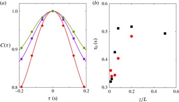
Figure 8(a) shows three examples of temperature autocorrelation functions for
 $\unicode[STIX]{x1D6E4}=0.50$
near their peaks. The Taylor series expansion
 $$\begin{eqnarray}C(\unicode[STIX]{x1D70F})=1-(\unicode[STIX]{x1D70F}/\unicode[STIX]{x1D70F}_{0})^{2}+(\unicode[STIX]{x1D70F}/\unicode[STIX]{x1D70F}_{1})^{4}+\cdots\end{eqnarray}$$
in even powers and up to fourth order in
 $\unicode[STIX]{x1D70F}$
yielded a satisfactory fit for
 $|\unicode[STIX]{x1D70F}|\leqslant 0.2$
s and is shown by the solid lines; this fit gave the desired
 $\unicode[STIX]{x1D70F}_{0}$
. Measurements for
 $\unicode[STIX]{x1D6E4}=1.00$
look similar and will not be shown. We note that there is no spurious peak at
 $\unicode[STIX]{x1D70F}=0$
, which would tend to occur if there were a significant contribution from experimental broad-band noise.
(a) Examples of autocorrelation functions as a function of the time delay
 $\unicode[STIX]{x1D70F}$
for
 $\unicode[STIX]{x1D709}=1.00$
for (from bottom to top) the three values
 $z/L=0.022$
, 0.050 and 0.500. The lines are least-squares fits of (5.2) to the data, adjusting
 $\unicode[STIX]{x1D70F}_{0}$
and
 $\unicode[STIX]{x1D70F}_{1}$
. These fits yielded
 $\unicode[STIX]{x1D70F}_{0}=0.331$
, 0.427 and 0.493 s for
 $z/L=0.022$
, 0.050 and 0.500, respectively. (b) Results for
 $\unicode[STIX]{x1D70F}_{0}$
as a function of
 $z/L$
for
 $\unicode[STIX]{x1D6E4}=0.50$
,
 $\unicode[STIX]{x1D709}=0.063$
(red circles) and
 $\unicode[STIX]{x1D709}=1.00$
(black squares) on linear scales. All results in this figure are for
 $Ra=1.67\times 10^{12}$
and
 $\unicode[STIX]{x1D6E4}=0.50$
.

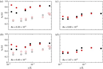
Results for
 $\unicode[STIX]{x1D70F}_{0}$
as a function of
 $z/L$
on logarithmic scales for
 $\unicode[STIX]{x1D709}=0.063$
(red circles) and
 $\unicode[STIX]{x1D709}=1.00$
(black squares): solid symbols,
 $\unicode[STIX]{x1D6E4}=0.50$
; open symbols,
 $\unicode[STIX]{x1D6E4}=1.00$
. In (a) the solid (open) symbols are for
 $\unicode[STIX]{x0394}T=3.00~\text{K}$
(
 $\unicode[STIX]{x0394}T=12.5~\text{K}$
) corresponding to
 $Ra=0.20\times 10^{12}$
(
 $Ra=0.20\times 10^{12}$
). In (b) the solid (open) symbols are for
 $\unicode[STIX]{x0394}T=6.00~\text{K}$
(
 $\unicode[STIX]{x0394}T=25.0~\text{K}$
) corresponding to
 $Ra=0.40\times 10^{12}$
(
 $Ra=0.42\times 10^{12}$
). In (c) the solid symbols are for
 $\unicode[STIX]{x0394}T=12~\text{K}$
corresponding to
 $Ra=0.8\times 10^{12}$
. In (d) the solid symbols are for
 $\unicode[STIX]{x0394}T=25~\text{K}$
corresponding to
 $Ra=1.67\times 10^{12}$
.

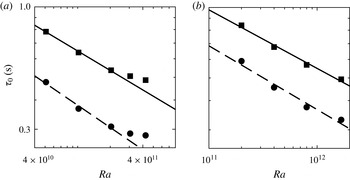
Results for
 $\unicode[STIX]{x1D70F}_{0}$
as a function of
 $Ra$
for
 $\unicode[STIX]{x1D709}=1.00$
: (a)
 $\unicode[STIX]{x1D6E4}=1.00$
; (b)
 $\unicode[STIX]{x1D6E4}=0.50$
. Squares:
 $z/L=0.50$
. Circles in (a):
 $z/L=0.034$
. Circles in (b):
 $z/L=0.022$
. The solid and dashed lines correspond to power laws with exponents of
 $-0.27$
and
 $-0.32$
, respectively, in (a) and
 $-0.25$
and
 $-0.27$
, respectively, in (b).

In figure 8(b) we show measurements of
 $\unicode[STIX]{x1D70F}_{0}$
as a function of
 $z/L$
for
 $\unicode[STIX]{x1D6E4}=0.50$
and
 $Ra=1.67\times 10^{12}$
on linear scales. Results for four values of
 $Ra$
and
 $\unicode[STIX]{x1D6E4}=0.50$
are given in figure 9 as solid symbols as a function of
 $z/L$
on logarithmic scales. The red circles are for
 $\unicode[STIX]{x1D709}=0.063$
(near the sidewall) and the black squares correspond to
 $\unicode[STIX]{x1D709}=1.00$
(along the vertical centreline). While figure 8(b) indicates that
 $\unicode[STIX]{x1D70F}_{0}$
initially increases with increasing
 $z/L$
, figure 9 makes it more obvious that the total variation over the sample height is less than a factor of 2. A similar mild dependence on
 $z/L$
was found also by Belmonte & Libchaber (Reference Belmonte and Libchaber1996), albeit for
 $Pr=0.7$
.
The results for
 $\unicode[STIX]{x1D70F}_{0}$
and
 $\unicode[STIX]{x1D6E4}=1.00$
are shown as open symbols in figure 9(a,b) and reveal a dependence on
 $z/L$
that is similar to what was seen for
 $\unicode[STIX]{x1D6E4}=0.50$
. At the same
 $Ra$
, the ratios of
 $\unicode[STIX]{x1D70F}_{0}$
for
 $\unicode[STIX]{x1D6E4}=0.50$
to those for
 $\unicode[STIX]{x1D6E4}=1.00$
range from approximately 1.7 near the plate to approximately 1.4 near the sample centre. We note that the ratio
 $R_{L}$
of the heights
 $L$
of the two samples is 1.58, i.e. close to these values. Thus, a dimensionless time
 $\unicode[STIX]{x1D70F}_{0}\unicode[STIX]{x1D705}/L^{2}$
turns out to decrease with increasing
 $\unicode[STIX]{x1D6E4}$
, for instance, very roughly as
 $\unicode[STIX]{x1D6E4}^{-0.5}$
at the sample centre.
The dependence of
 $\unicode[STIX]{x1D70F}_{0}$
on
 $Ra$
is illustrated in figure 10, where we show results for
 $\unicode[STIX]{x1D6E4}=1.00$
in (a) and for
 $\unicode[STIX]{x1D6E4}=0.50$
in (b). The squares are measured at the sample centre, while the circles are for a vertical position where
 $\unicode[STIX]{x1D70F}_{0}$
is close to its minimum value (
 $z/L=0.034$
for
 $\unicode[STIX]{x1D6E4}=1.00$
and
 $z/L=0.022$
for
 $\unicode[STIX]{x1D6E4}=0.50$
). Fits of power laws to the data give exponent values cited in the caption; all are in the range
 $-0.29\pm 0.04$
. The absolute values of these exponents are well below that reported for
 $Q(Ra)$
by Procaccia et al. (Reference Procaccia, Ching, Constantin, Kadanoff, Libchaber and Wu1991), who found
 $0.67$
for
 $Ra\lesssim 10^{11}$
and
 $\unicode[STIX]{x1D6E4}=0.50$
, albeit for
 $Pr\simeq 1$
. They are also smaller than the value obtained for
 $\unicode[STIX]{x1D70F}_{0}(Ra)$
for
 $Ra\lesssim 10^{11}$
by Belmonte & Libchaber (Reference Belmonte and Libchaber1996), who measured an exponent of
 $-0.68$
for
 $\unicode[STIX]{x1D6E4}=1.00$
, but also for
 $Pr=0.7$
, which is much smaller than ours. A theoretical/numerical estimate by Grossmann & Lohse (Reference Grossmann and Lohse1992) gives
 $0.58$
for the exponent of
 $Q(Ra)$
, which again is approximately a factor of 2 larger than our results; but it is not transparent to us how this estimate would depend on
 $Pr$
.
We note that the data in figure 10 tend to show systematic positive deviations at large
 $Ra$
from the power-law representations. There is some similarity to the results of Procaccia et al. (Reference Procaccia, Ching, Constantin, Kadanoff, Libchaber and Wu1991) for
 $Q$
, who found a smaller power-law exponent for
 $Ra\gtrsim 10^{11}$
than they measured for
 $Ra\lesssim 10^{11}$
. For that case, Grossmann & Lohse (Reference Grossmann and Lohse1993) argued that this change in
 $Ra$
dependence was caused by the finite response time and/or size of the temperature sensor. As discussed in § 4.1, we believe that the response of our thermistors is fast enough; but we cannot rule out completely that the arguments of Grossmann & Lohse (Reference Grossmann and Lohse1993) become relevant to our measurements for the smaller values of
 $\unicode[STIX]{x1D70F}_{0}$
.
5.4 The temperature probability distribution
5.4.1 The sample centre
As discussed in § 2, the turbulent background fluctuations, relatively unencumbered by plume and LSC contributions, are accessible only at the sample centre (
 $z/L=0.50$
,
 $\unicode[STIX]{x1D709}=1.00$
). Thus we focus first on measurements at this location.
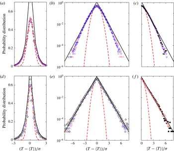
Probability distributions of temperature fluctuations
 $T-\langle T\rangle$
about their mean value
 $\langle T\rangle$
, scaled by the square root
 $\unicode[STIX]{x1D70E}$
of the variance
 $\unicode[STIX]{x1D70E}^{2}$
. Panels (a)–(c) are for
 $\unicode[STIX]{x1D6E4}=0.5$
, and (d)–(f) are for
 $\unicode[STIX]{x1D6E4}=1.00$
. All data are for the sample centre at
 $z/L=0.5,~\unicode[STIX]{x1D709}=1.00$
. Panels (a) and (d) are on linear scales, while the other panels have a logarithmic vertical scale. In (c) and (f), the data are plotted as a function of the absolute value
 $|T-\langle T\rangle |/\unicode[STIX]{x1D70E}$
of the abscissa, with the solid points corresponding to negative
 $T-\langle T\rangle$
. The dashed red lines are fits of the Gaussian function near the peak of the distribution. The solid lines are fits of an exponential function to data not too close to the peak. The data in (a) and (b) are for
 $Ra=16.6\times 10^{11}$
(downward-pointing triangles),
 $7.98\times 10^{11}$
(upward-pointing triangles),
 $3.99\times 10^{11}$
(circles) and
 $2.00\times 10^{11}$
(pluses). The data in (c) are for
 $Ra=16.6\times 10^{11}$
. The data in (d) and (e) are for
 $Ra=4.24\times 10^{11}$
(circles),
 $3.05\times 10^{11}$
(squares),
 $2.04\times 10^{11}$
(upward-pointing triangles),
 $1.02\times 10^{11}$
(downward-pointing triangles) and
 $0.51\times 10^{11}$
(diamonds). The data in (f) are for
 $Ra=4.24\times 10^{11}$
.

In figure 11 we show temperature probability distributions measured at the centre of the two samples. The upper panels are for
 $\unicode[STIX]{x1D6E4}=0.50$
, while the lower panels are for
 $\unicode[STIX]{x1D6E4}=1.00$
. Figures 11(a) and 11(d) are on linear scales, while the other panels have logarithmic vertical scales. In both cases, the sets with different symbols cover about a decade of
 $Ra$
. One sees that the shapes of the distributions, when plotted as a function of
 $(T-\langle T\rangle )/\unicode[STIX]{x1D70E}$
, are independent of
 $Ra$
, as found already by Castaing et al. (Reference Castaing, Gunaratne, Heslot, Kadanoff, Libchaber, Thomae, Wu, Zaleski and Zanetti1989) at
 $z/L=0.50,~\unicode[STIX]{x1D709}=0.50$
for
 $Pr$
close to one and by Du & Tong (Reference Du and Tong2001) at the sample centre for
 $Pr=5.4$
. Figures 11(c) and 11(f) show the data at one
 $Ra$
value as a function of the absolute value of
 $(T-\langle T\rangle )/\unicode[STIX]{x1D70E}$
. There, the solid (open) symbols are for negative (positive)
 $(T-\langle T\rangle )$
. The results illustrate that the distributions are symmetric about
 $(T-\langle T\rangle )=0$
, i.e. that the skewness is essentially zero. We note that the distributions of Castaing et al. (Reference Castaing, Gunaratne, Heslot, Kadanoff, Libchaber, Thomae, Wu, Zaleski and Zanetti1989) were noticeably skewed (see their figures 3b and 12). Although they were measured at
 $z/L=0.50,~\unicode[STIX]{x1D709}=0.5$
rather than at the sample centre (
 $\unicode[STIX]{x1D709}=1.00$
), our measurements do not reveal any significant radial dependence of the skewness
 $S$
(3.8) at
 $z/L=0.50$
(see figure 13
b below).
The distributions for
 $\unicode[STIX]{x1D6E4}=1.00$
(figure 11
d–f) can be described well by a double-exponential (or Laplace) distribution as indicated by the solid lines (in the physical system we expect that the exponential dependence breaks down near the peak in order for the function to be analytic). This also agrees with the finding of Castaing et al. (Reference Castaing, Gunaratne, Heslot, Kadanoff, Libchaber, Thomae, Wu, Zaleski and Zanetti1989) as well as others (e.g. Du & Tong Reference Du and Tong2001; He & Tong Reference He and Tong2009). For
 $\unicode[STIX]{x1D6E4}=0.50$
(figure 11
a–c), the double-exponential distribution is not as good an approximation, as seen also in the data of Du & Tong (Reference Du and Tong2001).
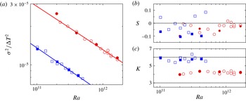
The scaled variance
 $\unicode[STIX]{x1D70E}^{2}/\unicode[STIX]{x0394}T$
(3.6), skewness
 $S$
(3.8) and kurtosis
 $K$
(3.10) at the sample centre as functions of
 $Ra$
: circles,
 $\unicode[STIX]{x1D6E4}=0.50$
; squares,
 $\unicode[STIX]{x1D6E4}=1.00$
; open (solid) symbols, long, slow (shorter, fast) time series (see § 4.2). In (a) the lines are fits of power laws to the open symbols, which yielded exponents of
 $-0.34\pm 0.01$
for
 $\unicode[STIX]{x1D6E4}=0.50$
and
 $-0.35\pm 0.02$
for
 $\unicode[STIX]{x1D6E4}=1.00$
. In (c) the horizontal dotted lines correspond to
 $K=3$
(Gaussian distribution) and
 $K=6$
(Laplace distribution).

A more quantitative description of the distributions is found in their moments. Figure 12 shows the variance
 $\unicode[STIX]{x1D70E}^{2}$
scaled by
 $\unicode[STIX]{x0394}T^{2}$
(3.6), the scaled skewness
 $S$
(3.8) and the scaled kurtosis
 $K$
(3.10) as a function of
 $Ra$
. Power-law fits to the open symbols show that
 $\unicode[STIX]{x1D70E}^{2}/\unicode[STIX]{x0394}T^{2}\sim Ra^{-0.35\pm 0.02}$
for
 $\unicode[STIX]{x1D6E4}=1.00$
and
 ${\sim}Ra^{-0.34\pm 0.01}$
for
 $\unicode[STIX]{x1D6E4}=0.50$
. For
 $Pr\simeq 1$
the exponent was measured by Castaing et al. (Reference Castaing, Gunaratne, Heslot, Kadanoff, Libchaber, Thomae, Wu, Zaleski and Zanetti1989) and found to be
 $-0.29\pm 0.01$
, i.e. with an absolute value slightly smaller than our value. The skewness
 $S$
is very close to zero as expected for the ideal RBC system at the sample centre. Averaging over the open symbols we find a mean value of
 $-0.025\pm 0.029$
for
 $\unicode[STIX]{x1D6E4}=0.50$
and
 $-0.001\pm 0.056$
for
 $\unicode[STIX]{x1D6E4}=1.00$
. Consistent with inspection of figure 11, the kurtosis
 $K$
for
 $\unicode[STIX]{x1D6E4}=1.00$
(
 $5.78\pm 0.29$
) is very close to the Laplace value of 6, while that for
 $\unicode[STIX]{x1D6E4}=0.50$
is significantly smaller (
 $4.18\pm 0.13$
), albeit larger than the Gaussian value of 3.
5.4.2 The horizontal midplane of the sample
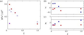
In figure 13(a) we show
 $\unicode[STIX]{x1D70E}^{2}/\unicode[STIX]{x0394}T^{2}$
as a function of radial position in the horizontal midplane
 $z/L=0.5$
. Here we see that
 $\unicode[STIX]{x1D70E}^{2}$
is much larger near the sidewall than near the sample centre, by a factor of approximately 5 for
 $\unicode[STIX]{x1D6E4}=1.00$
and of approximately 3 for
 $\unicode[STIX]{x1D6E4}=0.50$
. Again, we argue that the most likely explanation of this trend is that the contribution from the LSC dynamics to
 $\unicode[STIX]{x1D70E}^{2}$
becomes dominant near the wall, while it is absent or small near the sample centre. The purple solid square is the difference between the variance based on the measured temperature time series at
 $\unicode[STIX]{x1D709}=0.063$
,
 $z/L=0.50$
(also shown as an open square in figure 6) and the LSC dynamics contribution shown as a solid line in figure 6. One sees that this difference is of about the same size as the measured value at the sample centre.
(a) The scaled variance
 $\unicode[STIX]{x1D70E}^{2}/\unicode[STIX]{x0394}T^{2}$
, (b) the scaled skewness
 $S$
and (c) the scaled kurtosis
 $K$
as functions of radial position
 $\unicode[STIX]{x1D709}$
in the horizontal midplane (
 $z/L=0.50$
) for
 $\unicode[STIX]{x0394}T=25.0~\text{K}$
. Blue open squares:
 $\unicode[STIX]{x1D6E4}=1.00$
and
 $Ra=0.42\times 10^{12}$
. Red solid circles:
 $\unicode[STIX]{x1D6E4}=0.50$
and
 $Ra=1.67\times 10^{12}$
. Purple solid square:
 $\unicode[STIX]{x1D70E}^{2}-\unicode[STIX]{x1D70E}_{LSC}^{2}$
for
 $\unicode[STIX]{x1D6E4}=0.50$
,
 $Ra=1.67\times 10^{12}$
with
 $\unicode[STIX]{x1D70E}_{LSC}^{2}$
taken from figure 6.

Although near the sidewall there may be contributions to the probability distribution from plumes, which can raise the tails of the distribution, at
 $z/L=0.50$
in the ideal system one would expect the same number of cold and hot plumes, with an equal effect on the positive and negative tails. Thus the skewness
 $S$
(3.8) should remain close to zero. On the other hand, a significant contribution from plumes would be expected to broaden the distribution, thereby decreasing the kurtosis
 $K$
(3.10). In figure 13(b) and (c) we show
 $S$
and
 $K$
as a function of
 $\unicode[STIX]{x1D709}$
. As expected, one sees that
 $S$
remains quite small along the sample radius, with deviations from zero no larger than those seen at the sample centre (figure 12
b) as a function of
 $Ra$
. As expected, for
 $\unicode[STIX]{x1D6E4}=1.00$
the kurtosis did decrease from approximately 5.8 at the centre to 4.2 near the wall (blue squares in figure 13
c). But for
 $\unicode[STIX]{x1D6E4}=0.50$
,
 $K$
remained close to 4.2 along the entire radius.
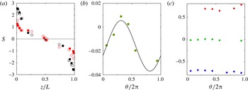
(a) The skewness
 $S=m_{3}/\unicode[STIX]{x1D70E}^{3/2}$
of the temperature probability distribution as a function of
 $z/L$
on linear scales: black squares,
 $\unicode[STIX]{x1D709}=1.00$
; red circles,
 $\unicode[STIX]{x1D709}=0.063$
; solid symbols,
 $\unicode[STIX]{x1D6E4}=0.50$
; open symbols,
 $\unicode[STIX]{x1D6E4}=1.00$
. (b) The skewness
 $S$
for
 $\unicode[STIX]{x1D6E4}=0.50$
as a function of azimuthal orientation
 $\unicode[STIX]{x1D703}/2\unicode[STIX]{x03C0}$
in the horizontal midplane (
 $z/L=0.50$
) near the sidewall at
 $\unicode[STIX]{x1D709}=0.063$
. (c) The skewness
 $S$
for
 $\unicode[STIX]{x1D6E4}=0.50$
and
 $\unicode[STIX]{x1D709}=0.063$
as a function of
 $\unicode[STIX]{x1D703}/2\unicode[STIX]{x03C0}$
at
 $z/L=0.25$
(red squares),
 $z/L=0.50$
(green circles) and
 $z/L=0.75$
(blue diamonds). All results in this figure are for
 $\unicode[STIX]{x0394}T=25.0~\text{K}$
, which corresponds to
 $Ra=1.67\times 10^{12}$
for
 $\unicode[STIX]{x1D6E4}=0.50$
and
 $Ra=0.42\times 10^{12}$
for
 $\unicode[STIX]{x1D6E4}=1.00$
.

5.4.3 The sample interior
It is instructive to examine the skewness (3.8) as a function of the vertical position because it is indicative of the presence of hot or cold excitations, i.e. of plumes – rising hot (falling cold) plumes would be expected to yield a positive (negative) skewness (see e.g. Belmonte & Libchaber Reference Belmonte and Libchaber1996).
The scaled skewness
 $S$
(3.8) for
 $\unicode[STIX]{x0394}T=25.0~\text{K}$
is shown in figure 14(a) as a function of
 $z/L$
. There the open (solid) symbols are for
 $\unicode[STIX]{x1D6E4}=1.00$
and
 $Ra=0.42\times 10^{12}$
(
 $\unicode[STIX]{x1D6E4}=0.50$
and
 $Ra=1.67\times 10^{12}$
). The results are surprisingly independent of
 $\unicode[STIX]{x1D6E4}$
. Along the centreline (black squares) one sees that
 $|S|$
becomes quite large near the plates (in the ‘inner layer’; see figure 22 below). It depends strongly on
 $z/L$
for
 $z/L\lesssim 0.2$
and
 $z/L\gtrsim 0.8$
and more gently closer to the sample centre (in the outer layer). The ranges of large
 $|S|$
more or less coincide with the ranges of significant
 $z/L$
dependence of
 $\unicode[STIX]{x1D70F}_{0}$
. In the central part of the sample, where
 $\unicode[STIX]{x1D70F}_{0}$
is nearly constant,
 $|S|$
is small. For a sample satisfying the Oberbeck–Boussinesq approximation (Oberbeck Reference Oberbeck1879; Boussinesq Reference Boussinesq1903),
 $S$
is expected to vanish at the sample centre. The actual value measured there was
 $-0.02$
. Near the sidewall (red circles)
 $|S|$
is smaller than it is along the centreline. A possible reason may be found in the broad distribution of the orientation
 $\unicode[STIX]{x1D703}_{0}$
of the LSC circulation plane (see figure 5
b). Since the plumes tend to travel with the LSC, they are (in the time average) also distributed azimuthally along the periphery of the sample. On average, only a fraction of them would then pass by a particular temperature sensor.
(a,b) The variance
 $\unicode[STIX]{x1D70E}^{2}$
, scaled by
 $(\unicode[STIX]{x0394}T)^{2}$
, as a function of
 $z/L$
on (a) double-logarithmic scales and (b) semi-logarithmic scales. (c) The square root
 $\unicode[STIX]{x1D70E}/\unicode[STIX]{x0394}T$
of the variance
 $\unicode[STIX]{x1D70E}^{2}/\unicode[STIX]{x0394}T^{2}$
versus
 $z/L$
on semi-logarithmic scales. (d)–(f) The ratio of the measured value to the fitted value corresponding to the panel above it. Red circles:
 $\unicode[STIX]{x1D709}=0.063$
. Black squares:
 $\unicode[STIX]{x1D709}=1.00$
. The data are for
 $\unicode[STIX]{x1D6E4}=0.50$
and
 $Ra=1.67\times 10^{12}$
.

The dependence of
 $S$
on the azimuthal coordinate
 $\unicode[STIX]{x1D703}/2\unicode[STIX]{x03C0}$
is shown in figures 14(b) and 14(c). Figure 14(b) shows the results in the horizontal midplane with high resolution. There, one sees that
 $S$
is close to zero at all angles with a mean value of
 $-0.015$
, but that some azimuthal variation due to the non-uniform distribution of
 $\unicode[STIX]{x1D703}_{0}$
remains. The distributions at
 $z/L=0.25$
, 0.50 and 0.75 are shown in figure 14(c) on a scale covering a wider range of
 $S$
. The preponderance of hot (cold) plumes in the bottom (top) of the sample at
 $z/L=0.25$
(
 $z/L=0.75$
) is evident. The azimuthal variation of
 $S$
is quite weak also away from the horizontal midplane, indicating a broad, nearly uniform, azimuthal distribution (in the time average) of rising and falling plumes.
5.5 The variance in the bulk near the plates, i.e. in the ‘inner’ layer
The TP model predicts that the variance
 $\unicode[STIX]{x1D70E}^{2}$
(see (3.6)) should depend logarithmically on
 $z/L$
(see (1.3)) and that the spectra (see § 5.6) have a power-law range (see (1.1)) with an exponent
 $\unicode[STIX]{x1D6FC}=1$
. As an example of the experimental results for
 $\unicode[STIX]{x1D70E}^{2}$
, we show data, scaled by
 $(\unicode[STIX]{x0394}T)^{2}$
, for
 $\unicode[STIX]{x1D6E4}=0.50$
and
 $Ra=1.67\times 10^{12}$
in figure 15. In figure 15(a) the measurements are shown on double-logarithmic scales and in figure 15(b) they are given on semi-logarithmic scales. The ratios of the measured values to the values of the fitted function are shown in figures 15(d) and 15(e). One sees that a power law (straight line in figure 15
a) is a much better fit to the data than a logarithmic dependence (straight line in figure 15
b), in disagreement with the TP model prediction. For other
 $Ra$
and
 $\unicode[STIX]{x1D6E4}=1.00$
, similar results were obtained. The favoured power-law dependence differs from the results for
 $Pr=0.8$
where a logarithmic function fitted the data very well for
 $z/L\lesssim 0.1$
(He et al.
Reference He, van Gils, Bodenschatz and Ahlers2014), in agreement with the TP model.
A fit of (1.2) to the data in figure 15(a) over the range
 $z/L\leqslant 0.10$
gave
 $\unicode[STIX]{x1D701}=0.63$
for
 $\unicode[STIX]{x1D709}=0.063$
(i.e. near the sidewall) and
 $\unicode[STIX]{x1D701}=0.96$
for
 $\unicode[STIX]{x1D709}=1.00$
(i.e. along the sample centreline). The result near the sidewall where most of the plumes rise or fall and where the LSC dynamics contributes most strongly agrees well with the Priestley prediction
 $\unicode[STIX]{x1D701}=2/3$
for convection over a heated horizontal surface. Along the centreline the exponent is close to the prediction
 $\unicode[STIX]{x1D701}=1$
based on one interpretation by Adrian (Reference Adrian1996) of a model by Castaing et al. (Reference Castaing, Gunaratne, Heslot, Kadanoff, Libchaber, Thomae, Wu, Zaleski and Zanetti1989). However, an alternative interpretation (Adrian Reference Adrian1996) of the model yields a logarithmic dependence of
 $\unicode[STIX]{x1D70E}$
(i.e. the square root of the variance) on
 $z/L$
, and, as seen in figures 15(c) and 15(f), such a dependence, while not quite as good a fit as a power law (figure 15
a,d), is difficult to rule out. Thus, some ambiguity remains regarding the dependence of the temperature fluctuation amplitude or intensity on
 $z/L$
. Unfortunately, the models due to Priestley (Reference Priestley1954) and Castaing et al. (Reference Castaing, Gunaratne, Heslot, Kadanoff, Libchaber, Thomae, Wu, Zaleski and Zanetti1989) to our knowledge make no statement about the spectra that could perhaps be compared more unambiguously with experiment as is the case for the TP model. And, of course, in view of the multiple contributions to
 $\unicode[STIX]{x1D70E}^{2}$
, there is no obvious reason why any of these models should agree with the data except perhaps along the sample centreline where the LSC dynamics is expected to contribute less and where the intrinsic fluctuations may be expected to dominate.
The exponent
 $\unicode[STIX]{x1D701}$
(see (1.2)) as a function of
 $Ra$
. Squares and circles:
 $\unicode[STIX]{x1D6E4}=0.5$
. Stars:
 $\unicode[STIX]{x1D6E4}=1.00$
. Solid (open) symbols were obtained near the bottom (top) plate.

In figure 16 we show the power-law exponent values for the two
 $\unicode[STIX]{x1D6E4}$
that were obtained from a fit of (1.2) to the data with
 $z/L<0.1$
as a function of
 $Ra$
. The circles and squares are for
 $\unicode[STIX]{x1D6E4}=0.50$
. Although these data scatter quite a bit, there is no evidence for a systematic dependence of
 $\unicode[STIX]{x1D701}$
on
 $Ra$
, and one clearly sees that
 $\unicode[STIX]{x1D701}\simeq 1$
(upper dotted line) along the sample centreline, where there are relatively few plumes, and
 $\unicode[STIX]{x1D701}\simeq 2/3$
(lower dotted line) near the sidewall, where most of the plumes rise or fall and where the LSC contributes strongly. An average over
 $Ra$
of all the
 $\unicode[STIX]{x1D701}$
values for
 $\unicode[STIX]{x1D709}=1.00$
and
 $\unicode[STIX]{x1D6E4}=0.50$
yielded
 $\unicode[STIX]{x1D701}=1.00\pm 0.05$
. For
 $\unicode[STIX]{x1D709}=0.063$
, this average was
 $0.69\pm 0.04$
.
Results for
 $\unicode[STIX]{x1D701}$
and
 $\unicode[STIX]{x1D6E4}=1.00$
are shown in figure 16 as stars. They are consistent with the
 $\unicode[STIX]{x1D6E4}=0.50$
data, although the results for
 $\unicode[STIX]{x1D709}=0.063$
suggest a slight increase with decreasing
 $Ra$
above the
 $2/3$
value.
5.6 The power spectra
The characteristic time
 $\unicode[STIX]{x1D70F}_{0}$
plays a role in the time domain that is analogous to that of the Taylor microscale (see e.g. Pope Reference Pope2000) in the spatial domain (He et al.
Reference He, van Gils, Bodenschatz and Ahlers2014, Reference He, van Gils, Bodenschatz and Ahlers2015). On the basis of the elliptic approximation (EA) of He & Zhang (Reference He and Zhang2006), it can be shown that there is a space–time equivalence when time is scaled with
 $\unicode[STIX]{x1D70F}_{0}$
and space is scaled with
 $\unicode[STIX]{x1D706}_{0}$
, where
 $\unicode[STIX]{x1D706}_{0}$
is obtained from a Taylor series expansion, analogous to (5.2), of the spatial autocorrelation function
 $C(z)$
(
 $z$
is the spatial displacement; see e.g. He et al.
Reference He, van Gils, Bodenschatz and Ahlers2015). This equivalence is expressed by the relationship
 $P(f\unicode[STIX]{x1D70F}_{0})=P(k\unicode[STIX]{x1D706}_{0})$
, where
 $k$
is the wavenumber. We shall make the frequencies of the power spectra dimensionless by multiplying with
 $\unicode[STIX]{x1D70F}_{0}$
. Thus, to the extent of the validity of the EA, these spectra are the same as the spatial power spectra
 $P(k\unicode[STIX]{x1D706}_{0})$
.
Normalized reduced power spectra
 $(f\unicode[STIX]{x1D70F}_{0})P(f\unicode[STIX]{x1D70F}_{0})$
on double-logarithmic scales for
 $\unicode[STIX]{x1D709}=1.00$
. Starting at the bottom, the sets are shifted vertically by factors of 1, 3, 5, 9, 14 and 20, respectively, for clarity. (a) Plots for
 $\unicode[STIX]{x1D6E4}=0.50$
,
 $\unicode[STIX]{x0394}T=25.0~\text{K}$
,
 $Ra=1.67\times 10^{12}$
and
 $\unicode[STIX]{x1D709}=1.00$
. From bottom to top, they are for
 $z/L=0.013,~0.022,~0.050,~0.080,~0.100$
and
 $0.500$
. (b) Plots for
 $\unicode[STIX]{x1D6E4}=1.00$
,
 $\unicode[STIX]{x0394}T=25.0~\text{K}$
,
 $Ra=0.42\times 10^{12}$
and
 $\unicode[STIX]{x1D709}=1.00$
. From bottom to top, they are for
 $z/L=0.016,~0.034,~0.053,~0.095,~0.263$
and
 $0.500$
. (c) Plots for
 $\unicode[STIX]{x1D6E4}=0.50$
,
 $\unicode[STIX]{x0394}T=25.0~\text{K}$
,
 $Ra=1.67\times 10^{12}$
and
 $\unicode[STIX]{x1D709}=0.063$
, for
 $z/L$
as in (a). (d) Plots for
 $\unicode[STIX]{x1D6E4}=1.00$
,
 $\unicode[STIX]{x0394}T=25.0~\text{K}$
,
 $Ra=0.42\times 10^{12}$
and
 $\unicode[STIX]{x1D709}=0.063$
for
 $z/L$
as in (b).

(a,b) The power-law exponent
 $\unicode[STIX]{x1D6FC}$
of the power spectra as a function of
 $z/L$
or
 $1-z/L$
for
 $\unicode[STIX]{x0394}T=25.0~\text{K}$
,
 $Ra=1.67\times 10^{12}$
and
 $\unicode[STIX]{x1D6E4}=0.50$
. Red circles:
 $\unicode[STIX]{x1D709}=0.063$
. Black squares:
 $\unicode[STIX]{x1D709}=1.00$
. Solid symbols:
 $z/L\leqslant 0.5$
. Open symbols:
 $z/L>0.5$
. Panel (a) shows the data on a logarithmic horizontal scale, while for (b) both axes have linear scales. (c,d) Data similar to those in (a) and (b), but for
 $\unicode[STIX]{x1D6E4}=1.00$
,
 $\unicode[STIX]{x0394}T=25.0~\text{K}$
and
 $Ra=0.42\times 10^{12}$
. The dotted horizontal lines in (a) and (c) indicate the value
 $\unicode[STIX]{x1D6FC}=1$
expected in the near-plate region
 $z/L\lesssim 0.1$
on the basis of the TP model.

In figure 17 we show spectra in the reduced form
 $(f\unicode[STIX]{x1D70F}_{0})P(f\unicode[STIX]{x1D70F}_{0})$
as a function of
 $f\unicode[STIX]{x1D70F}_{0}$
on double-logarithmic scales. For clarity, the spectra are shifted vertically relative to each other by the factors given in the caption, with the bottom spectrum (at the smallest
 $z/L$
) unshifted. The results in figures 17(a) and 17(b) are for
 $\unicode[STIX]{x1D709}=1.00$
; and (a) is for
 $\unicode[STIX]{x1D6E4}=0.50$
and
 $Ra=1.67\times 10^{12}$
while (b) is for
 $\unicode[STIX]{x1D6E4}=1.00$
and
 $Ra=0.42\times 10^{12}$
. The spectra for
 $\unicode[STIX]{x1D6E4}=1.00$
(figure 17
b) clearly show the low-frequency peak due to the LSC oscillations discussed above in § 4.2, but the results in figure 17(a) for
 $\unicode[STIX]{x1D6E4}=0.50$
show little or no evidence for such a peak. In § 5.1 above we showed that the LSC amplitude
 $\unicode[STIX]{x1D6FF}_{m}$
at the same
 $Ra$
is nearly the same for the two
 $\unicode[STIX]{x1D6E4}$
values. Thus it seems that for
 $\unicode[STIX]{x1D6E4}=0.50$
the torsional and/or sloshing mode of the LSC is absent or weak. For each spectrum one sees that there is a range covering about a decade of
 $f\unicode[STIX]{x1D70F}_{0}$
over which it can be described well by the power law (1.1).
The power-law exponent
 $\unicode[STIX]{x1D6FC}$
for
 $\unicode[STIX]{x1D6E4}=0.50$
and
 $Ra=1.67\times 10^{12}$
is given in figures 18(a) and 18(b) as a function of
 $z/L$
. The red circles and black squares are for
 $\unicode[STIX]{x1D709}=0.063$
and
 $\unicode[STIX]{x1D709}=1.00$
, respectively. Corresponding results for
 $\unicode[STIX]{x1D6E4}=1.00$
and
 $Ra=0.42\times 10^{12}$
are shown in figures 18(c) and 18(d). One sees for both
 $\unicode[STIX]{x1D6E4}$
that there is no range of
 $z/L$
over which
 $\unicode[STIX]{x1D6FC}=1.00$
. This result differs from the
 $Pr=0.8$
case, where
 $\unicode[STIX]{x1D6FC}=1.00$
was found for
 $\unicode[STIX]{x1D6E4}=0.5$
and
 $0.01\lesssim z/L\lesssim 0.1$
(He et al.
Reference He, van Gils, Bodenschatz and Ahlers2014). At both radial locations,
 $\unicode[STIX]{x1D6FC}$
initially increased roughly logarithmically with
 $z/L$
, although a power law with an exponent between 0.2 and 0.3 is also a good representation of the data.
Along the vertical sample centreline (
 $\unicode[STIX]{x1D709}=1.00$
) and for both
 $\unicode[STIX]{x1D6E4}$
, the exponent approaches its maximum value
 $\unicode[STIX]{x1D6FC}=1.27\pm 0.01$
as
 $z/L$
approaches
 $0.5$
(see also figure 1
a). This result is well below the value
 $5/3$
of Obukhov–Corrsin scaling for passive scalars (Obukhov Reference Obukhov1949; Corrsin Reference Corrsin1951) and also smaller than the value
 $7/5$
suggested by Bolgiano (Reference Bolgiano1959) and Obukhov (Reference Obukhov1959) for stably stratified convection – see Lohse & Xia (Reference Lohse and Xia2010) for a more detailed discussion. However, as we shall show below in figure 21(b),
 $\unicode[STIX]{x1D6FC}$
at the sample centre is still increasing with increasing
 $Ra$
and thus is expected to be smaller than the high-Reynolds-number value envisioned by the theories. It is also smaller than the values near 1.5 obtained, for instance, by Niemela et al. (Reference Niemela, Skrbek, Sreenivasan and Donnelly2000) for
 $\unicode[STIX]{x1D6E4}=0.50$
at the sample centre for
 $Pr\simeq 0.7$
and
 $Ra\simeq 6\times 10^{11}$
. Apparently, for
 $Pr=12.3$
, the large-Reynolds-number regime had not yet been reached even for
 $Ra$
as large as
 $1.7\times 10^{12}$
.
Near the sidewall,
 $\unicode[STIX]{x1D6FC}$
reached a larger value, closer to 1.5, at
 $z/L=0.50$
; but we think it inappropriate to compare this result with the Bolgiano–Obukhov or Obukhov–Corrsin prediction because, as discussed in § 5.1, near the wall the LSC dynamics will contribute significantly to the spectrum. This value is, however, close to the results derived, for instance, from the data of He et al. (Reference He, van Gils, Bodenschatz and Ahlers2014) for
 $Pr=0.8$
,
 $\unicode[STIX]{x1D6E4}=0.50$
,
 $z/L=0.493$
and
 $\unicode[STIX]{x1D709}=0.018$
, which were
 $\unicode[STIX]{x1D6FC}=1.43$
for
 $Ra=1.08\times 10^{15}$
and
 $1.52$
for
 $Ra=1.63\times 10^{13}$
.
Power spectra, reduced by the factor
 $(f\unicode[STIX]{x1D70F}_{0})^{1.35}$
, as a function of
 $f\unicode[STIX]{x1D70F}_{0}$
at various radial positions
 $\unicode[STIX]{x1D709}$
and in the horizontal midplane at
 $z/L=0.50$
for (a)
 $\unicode[STIX]{x1D6E4}=1.00$
and (b)
 $\unicode[STIX]{x1D6E4}=0.50$
. In (a) the spectra are, from bottom to top, for
 $\unicode[STIX]{x1D709}=1.00$
, 0.25, 0.126 and 0.063. In (b) they are for
 $\unicode[STIX]{x1D709}=1.00$
, 0.32, 0.115 and 0.063. In both (a) and (b) the spectra are, from bottom to top, shifted upwards by the factors 1, 3, 5 and 9 to avoid overlap.

Figure 19 shows the spectra, reduced by the (arbitrarily chosen) factor
 $(f\unicode[STIX]{x1D70F}_{0})^{1.35}$
, as a function of
 $f\unicode[STIX]{x1D70F}_{0}$
for several radial locations in the horizontal midplane (
 $z/L=0.50$
) and for both
 $\unicode[STIX]{x1D6E4}$
. The spectra illustrate the gradual change with radial location of the exponent
 $\unicode[STIX]{x1D6FC}$
. For
 $\unicode[STIX]{x1D6E4}=1.00$
they also reveal the growth with distance from the sample centre of the sloshing/torsional mode contribution.
In figure 20 we show
 $\unicode[STIX]{x1D6FC}$
as a function of the radial position
 $\unicode[STIX]{x1D709}$
in the horizontal midplane. One sees that for both
 $\unicode[STIX]{x1D6E4}$
the exponent increases as the location of the measurement approaches the sidewall. We consider it likely that this increase is caused by the contribution from the stochastic dynamics of the LSC discussed above in § 5.1.
The power-law exponent
 $\unicode[STIX]{x1D6FC}$
of the power spectra as a function of radial position
 $\unicode[STIX]{x1D709}$
in the horizontal midplane (
 $z/L=0.50$
) for
 $\unicode[STIX]{x0394}T=25.0~\text{K}$
. Open squares:
 $\unicode[STIX]{x1D6E4}=0.50$
and
 $Ra=1.67\times 10^{12}$
. Solid circles:
 $\unicode[STIX]{x1D6E4}=1.00$
and
 $Ra=0.42\times 10^{12}$
.

(a) The power-law exponent
 $\unicode[STIX]{x1D6FC}$
of the power spectra for
 $\unicode[STIX]{x1D6E4}=0.50$
as a function of
 $z/L$
for
 $Ra=0.20\times 10^{12}$
. Red circles:
 $\unicode[STIX]{x1D709}=0.063$
. Black squares:
 $\unicode[STIX]{x1D709}=1.00$
. The dotted horizontal line indicates the value
 $\unicode[STIX]{x1D6FC}=1$
expected in the near-plate region
 $z/L\lesssim 0.1$
on the basis of the TP model. (b) The exponent
 $\unicode[STIX]{x1D6FC}$
for
 $\unicode[STIX]{x1D6E4}=0.50$
(solid squares) and
 $\unicode[STIX]{x1D6E4}=1.00$
(open squares) at the sample centre (
 $z/L=0.50$
and
 $\unicode[STIX]{x1D709}=1.00$
) as a function of
 $Ra$
. The solid (dashed) line is a power law with an exponent of 0.08 (0.16). The horizontal dotted (dash–dotted) line is the high-Reynolds-number Bolgiano–Obukhov (Obukhov–Corrsin) value
 $7/5$
(
 $5/3$
).

At other values of
 $Ra$
, similar results are found, as illustrated in figure 21(a) for
 $Ra=0.20\times 10^{12}$
. However, with decreasing
 $Ra$
and at constant
 $z/L$
, the
 $\unicode[STIX]{x1D6FC}$
value becomes smaller. For the results at the sample centre (
 $z/L=0.50$
and
 $\unicode[STIX]{x1D709}=1.00$
), this is illustrated in figure 21(b). A similar
 $Ra$
dependence was seen before, albeit for
 $Pr\simeq 0.7$
, by Sano et al. (Reference Sano, Wu and Libchaber1989), but apparently not by Wu et al. (Reference Wu, Kadanoff, Libchaber and Sano1990) for
 $Pr$
near 0.7 and by Zhou & Xia (Reference Zhou and Xia2001) for
 $Pr\simeq 4.3$
.
The
 $Ra$
dependence of
 $\unicode[STIX]{x1D6FC}$
at the sample centre suggests that the local fluctuation Reynolds number at that location is not yet high enough for
 $\unicode[STIX]{x1D6FC}$
to have reached the value appropriate for the large-
 $Ra$
limit and suitable for comparison with the theoretical arguments of Obukhov (Reference Obukhov1949) and Corrsin (Reference Corrsin1951) or of Bolgiano (Reference Bolgiano1959) and Obukhov (Reference Obukhov1959). It is worthwhile to look at this issue more closely even though we have no direct measurements of Reynolds numbers. At our largest
 $Ra=0.42\times 10^{12}$
for
 $\unicode[STIX]{x1D6E4}=1.00$
, and for
 $Pr=12.3$
, the measurements of Lam et al. (Reference Lam, Shang, Zhou and Xia2002) yield
 $Re_{V}=VL/\unicode[STIX]{x1D708}=4340$
, where
 $V$
is the root-mean-square fluctuation velocity. For our
 $\unicode[STIX]{x1D708}$
and
 $L$
, this corresponds to
 $V=7.2~\text{mm}~\text{s}^{-1}$
. Using our measured
 $\unicode[STIX]{x1D70F}_{0}=0.49$
s, the space–time equivalence (He et al.
Reference He, van Gils, Bodenschatz and Ahlers2015) based on the elliptic approximation of He & Zhang (Reference He and Zhang2006) gives a Taylor microscale
 $\unicode[STIX]{x1D706}_{0}=\unicode[STIX]{x1D70F}_{0}V=3.5$
mm. This length scale, and the above-mentioned
 $Re_{V}$
, yields
 $R_{\unicode[STIX]{x1D706}}\simeq 63$
, which is indeed quite small. For comparison, we note that the analogous exponent of temperature spectra in shear flow with various heat sources (see e.g. the compilation of many measurements by Sreenivasan (Reference Sreenivasan1996)) does not reach an asymptotic value near
 $5/3$
until
 $R_{\unicode[STIX]{x1D706}}$
becomes as large as 2000 or so. For the smallest
 $R_{\unicode[STIX]{x1D706}}\simeq 200$
of the shear-flow experiments, exponent values near 1.3 were found, which is not inconsistent with our RBC result. A more systematic study of the
 $R_{\unicode[STIX]{x1D706}}$
dependence of
 $\unicode[STIX]{x1D6FC}$
for RBC, with attention given to a possible
 $Pr$
dependence, would be of interest. For now it seems clear that it will not be easy to reach asymptotic values, with
 $R_{\unicode[STIX]{x1D706}}\gtrsim 2000$
, with large-
 $Pr$
fluids.
Finally, we remark on an interesting issue regarding large-
 $Pr$
temperature spectra examined theoretically by Batchelor (Reference Batchelor1959) and by Kraichnan (Reference Kraichnan1968, Reference Kraichnan1974). For large
 $Pr$
, these authors argue that there is a range of intermediate length scales over which the large viscosity still assures that the velocity field remains smooth while the small thermal diffusivity (or mass diffusivity) permits the temperature field (or that of a passive scalar) to develop more complex structures. They predict that the temperature spectrum, which according to their calculations has a
 $k^{-5/3}$
dependence at small
 $k$
, will develop an intermediate
 $k^{-1}$
range before the exponential decay due to dissipation setting in at even larger
 $k$
. This issue was addressed by Grossmann & Lohse (Reference Grossmann and Lohse1997), who calculated the fractal dimensions corresponding to a ‘wrinkled’ temperature field and found the
 $k^{-1}$
regime numerically for large enough
 $Pr$
. One might argue that for our
 $Pr=12.3$
this large-
 $Pr$
phenomenon might have been observed; but our data show no evidence for it. There may be several reasons for this; but the most likely one seems to be that, again, large
 $R_{\unicode[STIX]{x1D706}}\gtrsim 10^{3}$
would be required for the theoretical predictions to be applicable. Another reason may be that the
 $k^{-1}$
range is predicted to cover only a factor of
 $Pr^{1/2}$
(
 $\simeq 3.5$
in our case) along the
 $k$
axis (Batchelor Reference Batchelor1959). The transitions from the ‘inertial’ (in our case
 $k^{-1.24}$
) range to the
 $k^{-1}$
range and then to the exponentially decaying dissipative range are rounded and this rounding may well obscure the
 $k$
dependence of interest.
6 Comparison with previous experimental results and theoretical models
6.1 Historical background
Measurements of the mean temperature and of the temperature variance in thermal convection as a function of distance from the plates has a long history (for a summary of much of the early work, see e.g. Adrian, Ferreira & Boberg (Reference Adrian, Ferreira and Boberg1986)). However, to our knowledge, measurements of power spectra for RBC were reported first by Ahlers & Graebner (Reference Ahlers and Graebner1972), shortly after (relatively primitive) automated data acquisition became available (for a review, see Wonsiewicz, Storm & Sieber (Reference Wonsiewicz, Storm and Sieber1978)) and made it feasible to collect sufficiently long time series. The rediscovery a few years earlier of Gauss’ fast-Fourier-transform algorithm by Cooley & Tukey (Reference Cooley and Tukey1965) (for a review, see e.g. Heideman, Johnson & Burrus (Reference Heideman, Johnson and Burrus1984)) and the availability of early versions of digital computers like the PDP-11 series had only recently made it practical for experimentalists to compute spectra. More details of that and related work were given by Ahlers (Reference Ahlers1972, Reference Ahlers1974, Reference Ahlers and Riste1975), Ahlers & Behringer (Reference Ahlers and Behringer1978), Ahlers & Walden (Reference Ahlers and Walden1980) and Greenside et al. (Reference Greenside, Ahlers, Hohenberg and Walden1982); but those experiments were only for
 $Ra$
up to
 $3\times 10^{5}$
. It is now known that, for the relevant
 $Pr\simeq 0.7$
, the transition from chaotic patterns to turbulent convection occurs near the upper limit of the explored
 $Ra$
range (see e.g. the supplement to Bosbach, Weiss & Ahlers (Reference Bosbach, Weiss and Ahlers2012)); thus the measurements were for spatio-temporal chaos rather than for turbulence (see also e.g. Heslot, Castaing & Libchaber (Reference Heslot, Castaing and Libchaber1987)). The spectra were those of
 $Nu$
at a constant imposed heat current
 $Q$
. For modest values of
 $\unicode[STIX]{x1D6E4}$
, they had a constant value (white noise) at low frequencies and then decayed with a power-law exponent of
 $-4.0\pm 0.2$
. This exponent is characteristic of the solutions of two coupled first-order stochastically driven ordinary differential equations (Frish & Morph Reference Frish and Morph1981) and typical for a low-dimensional chaotic system (a relevant theoretical case would be, for instance, a Lorenz model (Lorenz Reference Lorenz1963) with added noise; see also Greenside et al. (Reference Greenside, Ahlers, Hohenberg and Walden1982)). Thus, the report by Ahlers & Graebner (Reference Ahlers and Graebner1972) to our knowledge provides the first experimental documentation of the occurrence of chaos in a continuum system, i.e. a system described by a partial differential equation (the Navier–Stokes equation).
The work was done with helium gas or liquid below approximately 5 K where, at sufficiently high pressures, large values of
 $Ra$
can be obtained in samples of modest height while using values of
 $\unicode[STIX]{x0394}T$
sufficiently small to assure near-Boussinesq conditions (Boussinesq Reference Boussinesq1903; Oberbeck Reference Oberbeck1879). For some parameter ranges in this system,
 $Pr$
can vary, but will remain in the range from 0.67 to 1.0 provided the critical point is not approached too closely. The merits of low-temperature helium for RBC studies were exploited independently at about the same time by Threlfall (Reference Threlfall1975), who reached much larger
 $Ra$
values up to approximately
 $2\times 10^{9}$
, well into the turbulent regime, but primarily reported on Nusselt-number measurements and did not present any spectra. While this early work was soon followed by spectral studies of other chaotic states obtained by using helium at low temperatures (see e.g. Libchaber & Maurer Reference Libchaber and Maurer1978; Maurer & Libchaber Reference Maurer and Libchaber1979, Reference Maurer and Libchaber1980), so far as we know spectral measurements in the turbulent regime were first made by Heslot et al. (Reference Heslot, Castaing and Libchaber1987). More detailed reviews of this early period were presented by Ahlers (Reference Ahlers, Brey, Marro, Rubi and San Miguel1995) and Aubin & Dalmedico (Reference Aubin and Dalmedico2002).
6.2 Fluctuation spectra and intensities near the horizontal midplane
For samples with
 $\unicode[STIX]{x1D6E4}$
near one, measurements at the sample centre are least likely to be influenced by the LSC and by plumes, and thus are most likely to be amenable to theoretical interpretation in terms of tractable models and simple assumptions. Thus we shall focus here first on results obtained in the horizontal midplane (
 $z/L=0.50$
) of the sample, where preferably one would like to consider data obtained at the sample centre (
 $\unicode[STIX]{x1D709}=1.00$
). In view of our finding of a significant
 $\unicode[STIX]{x1D709}$
dependence of both the spectra (figures 19 and 20) and the variance (figure 13), the interpretation of measurements at radial locations away from the centre must be done with caution.
Heslot et al. (Reference Heslot, Castaing and Libchaber1987) used helium gas near 4 K, and measured the local temperature near but not at the sample centre (
 $\unicode[STIX]{x1D709}=0.5$
,
 $z/L=0.50$
) of a sample with
 $\unicode[STIX]{x1D6E4}=1.0$
. They also made measurements for
 $z/L\simeq 0.002$
, but since these are likely to be in the boundary or buffer layer (also known as mixing layer), and since the probe size was comparable to
 $z/L$
, we shall not consider them further. Although
 $Pr$
was not reported, it most likely was near
 $0.7$
. Their spectra revealed a frequency range over which a power law described the results very well, and they found
 $\unicode[STIX]{x1D6FC}=1.4\pm 0.1$
at
 $Ra=4\times 10^{9}$
. While this result is consistent with the Bolgiano–Obukhov value
 $7/5$
(Bolgiano Reference Bolgiano1959; Obukhov Reference Obukhov1959) for stably stratified convection (see Lohse & Xia (Reference Lohse and Xia2010) for a more detailed discussion), this was not emphasized by the authors. Although measurements apparently were made up to
 $Ra\simeq 10^{11}$
, results for
 $\unicode[STIX]{x1D6FC}$
as a function of
 $Ra$
are not reported. The value for
 $\unicode[STIX]{x1D6FC}$
is considerably larger than ours; at our smallest
 $Ra\simeq 10^{11}$
, our result is only slightly larger than one, and we have no way of estimating its value near
 $Ra=4\times 10^{9}$
. Presumably the main reason for this large difference will be found in the large difference of
 $Pr$
.
A little later an
 $Ra$
-dependent
 $\unicode[STIX]{x1D6FC}$
was found by Sano et al. (Reference Sano, Wu and Libchaber1989) in the horizontal midplane (
 $z/L=0.50$
) at several radial positions with
 $\unicode[STIX]{x1D709}\leqslant 0.23$
for a sample with
 $\unicode[STIX]{x1D6E4}=1.00$
. That work used helium gas at a temperature near 5 K, which probably had a
 $Pr$
that increased with increasing pressure but probably was less than
 $1.1$
for
 $Ra\lesssim 10^{11}$
(see Castaing et al.
Reference Castaing, Gunaratne, Heslot, Kadanoff, Libchaber, Thomae, Wu, Zaleski and Zanetti1989), although
 $Pr$
is not given in the paper by Sano et al. (Reference Sano, Wu and Libchaber1989). The exponent values found for those parameters were reported to be independent of
 $\unicode[STIX]{x1D709}$
over the range of
 $\unicode[STIX]{x1D709}$
covered by the measurements (which differs from our finding for
 $Pr=12.3$
; see figure 20), and larger than those measured by us. Near
 $10^{11}$
, where a direct comparison is possible, Sano et al. (Reference Sano, Wu and Libchaber1989) found
 $\unicode[STIX]{x1D6FC}\simeq 1.42$
(see their figure 11) while at that
 $Ra$
and at the sample centre we have
 $\unicode[STIX]{x1D6FC}\simeq 1.05$
. Again, we believe that the most likely reason for this large difference is the difference in
 $Pr$
. As discussed above and illustrated in figure 21, we expect that their value of
 $\unicode[STIX]{x1D6FC}$
may also have been influenced by the LSC dynamics. It is surprising that these authors report an
 $Ra$
dependence of
 $\unicode[STIX]{x1D6FC}$
, while Heslot et al. (Reference Heslot, Castaing and Libchaber1987) for a nearly identical experiment made no mention of this and found
 $\unicode[STIX]{x1D6FC}\simeq 1.4$
for
 $Ra$
as small as
 $Ra=4\times 10^{9}$
where Sano et al. (Reference Sano, Wu and Libchaber1989) find
 $\unicode[STIX]{x1D6FC}\simeq 1.3$
.
In contradistinction to the results of Sano et al. (Reference Sano, Wu and Libchaber1989), an extensive study by Wu et al. (Reference Wu, Kadanoff, Libchaber and Sano1990) of spectra at the sample centre (
 $\unicode[STIX]{x1D709}=1.0$
,
 $z/L=0.50$
), also for helium gas at 5 K but for
 $\unicode[STIX]{x1D6E4}=0.50$
, finds
 $\unicode[STIX]{x1D6FC}=1.40\pm 0.05$
, independent of
 $Ra$
for
 $Ra$
not too small and up to approximately
 $10^{11}$
. So far as we can tell, the only significant differences between the two systems are the aspect ratio and the radial location (value of
 $\unicode[STIX]{x1D709}$
) of the measurement. However, while Wu et al. (Reference Wu, Kadanoff, Libchaber and Sano1990) find no
 $Ra$
dependence of
 $\unicode[STIX]{x1D6FC}$
for their
 $\unicode[STIX]{x1D6E4}=0.50$
sample, we do find a significant
 $Ra$
dependence for
 $\unicode[STIX]{x1D6E4}=0.50$
(see figure 21
b), albeit at the larger
 $Pr=12.3$
.
Spectral measurements at the centre of a sample with
 $\unicode[STIX]{x1D6E4}=0.50$
were made by Niemela et al. (Reference Niemela, Skrbek, Sreenivasan and Donnelly2000), also using helium at low temperatures, where
 $Pr\simeq 0.7$
. For
 $Ra=6\times 10^{11}$
their spectra were consistent with an exponent of 1.4 over a low-frequency range, consistent with Bolgiano–Obukhov scaling (Bolgiano Reference Bolgiano1959; Obukhov Reference Obukhov1959) for stably stratified convection. However, with increasing frequency, the curve became steeper and was interpreted by the authors to reveal Obukhov–Corrsin scaling for passive scalars (Obukhov Reference Obukhov1949; Corrsin Reference Corrsin1951) with an exponent near
 $5/3$
. Clearly, it is difficult to arrive at an unambiguous interpretation under these circumstances where the frequency range over which a given power law is observed is quite limited and the spectra decay even more rapidly as the frequency increases further and dissipation takes over. However, it is clear that the values of
 $\unicode[STIX]{x1D6FC}$
obtained by these authors are significantly larger than
 $\unicode[STIX]{x1D6FC}\simeq 1.3$
found by us at similar
 $Ra$
and at the larger
 $Pr=14.3$
(see figure 21
b).
Another remarkable set of measurements is that by Zhou & Xia (Reference Zhou and Xia2001) for
 $\unicode[STIX]{x1D6E4}=1.00$
at
 $Pr\simeq 4.3$
. At the sample centre, they found that
 $\unicode[STIX]{x1D6FC}$
was consistent with the Bolgiano–Obukhov value
 $7/5$
over a wide
 $Ra$
range from
 $2\times 10^{9}$
to
 $10^{11}$
, although individual exponent values are not shown.
An interesting set of measurements, but in a different geometry, was carried out by Fernandez & Adrian (Reference Fernandez and Adrian2002). Their sample had a square horizontal cross-section and aspect ratios (width/height) of 7.7. For
 $10^{8}\lesssim Ra\lesssim 2\times 10^{9}$
and
 $4.0\leqslant Pr\leqslant 6.7$
, they found in the horizontal midplane that the temperature probability distribution was close to a Laplace (bilateral exponential) distribution, as found in many investigations (including the present one; see figure 11) at large
 $Ra$
. At the larger
 $Ra$
the power spectra of the temperature fluctuations developed a frequency range over which they could be described by a power law with
 $\unicode[STIX]{x1D6FC}=1.4$
; but at lower frequencies a smaller exponent also could fit the data. Although the lateral position of the measurements was not given, we expect that the results are not sensitive to that location when the aspect ratio is large and the LSC structure can diffuse laterally. However, as discussed above, that diffusion would be expected to contribute to the fluctuations. The interpretation
 $\unicode[STIX]{x1D6FC}=1.4$
would agree with the measurements of Zhou & Xia (Reference Zhou and Xia2001) for similar
 $Pr$
and
 $\unicode[STIX]{x1D6E4}=1.00$
, and with the Bolgiano–Obukhov value
 $7/5$
; but their value of
 $\unicode[STIX]{x1D6FC}$
is larger than those found by us for
 $Pr=12.3$
(see figure 20).
6.3 Spatial dependence of fluctuation spectra and intensities in the near-plate region
In view of the complex nature of fluctuations in turbulent RBC, with contributions from intrinsic fluctuations, plumes and the LSC dynamics, one would not necessarily expect that any model of the system proposed so far would be adequate to catch the physics of all contributions. Nonetheless, here we compare model predictions with experimental data in attempts to provide some insight into the rich phenomena.
It is helpful to illustrate the various regions of turbulent RBC by considering the temperature profile shown by Ahlers et al. (Reference Ahlers, Bodenschatz and He2014) for
 $Ra=2\times 10^{12}$
and
 $Pr=0.8$
as is done in figure 22. The four layers shown there (boundary, buffer, log and outer layers) are analogous to those used by Chung et al. (Reference Chung, Yun and Adrian1992) (see their figure 1), albeit with different names. They also are analogous to the layers invoked typically in turbulent wall-bounded shear flow. All of the measurements of the present paper are in the inner (or ‘log’) layer (referred to as the ‘convection layer’ by Chung et al. (Reference Chung, Yun and Adrian1992)) and the outer layer (called the ‘buoyancy defect layer’ by Chung et al. (Reference Chung, Yun and Adrian1992)).
The profile shown in figure 22 is for
 $Ra=2\times 10^{12}$
, which is within the range of our
 $Ra$
for
 $\unicode[STIX]{x1D6E4}=0.50$
. Although
 $Pr$
for the present study is larger than that for figure 22 by a factor of 15, we expect that the inner (thermal) length scale
 $\unicode[STIX]{x1D706}_{th}=L/(2Nu)$
used along the upper abscissa is not very different for our sample since
 $Nu$
is only very weakly dependent on
 $Pr$
. One sees that the thermal BL (defined here as the range over which the pure conduction profile is a good approximation) extends approximately to
 $z/\unicode[STIX]{x1D706}_{th}=0.4$
. The thermal buffer layer follows and extends out to
 $z/\unicode[STIX]{x1D706}_{th}\simeq 8$
. Beyond the buffer layer, there is the ‘inner’ or ‘log’ layer, where the time-averaged temperature has a logarithmic dependence on
 $z$
(Ahlers et al.
Reference Ahlers, Bodenschatz, Funfschilling, Grossmann, He, Lohse, Stevens and Verzicco2012, Reference Ahlers, Bodenschatz and He2014; Wei & Ahlers Reference Wei and Ahlers2014). The buffer layer thus is a range where a gradual transition from the pure conduction to the logarithmic temperature profile takes place. The log layer extends out to
 $z/\unicode[STIX]{x1D706}_{th}$
as large as 200 or so and is followed by the outer layer, which is symmetric about the horizontal midplane and occupies the major part of the sample.
The dimensionless temperature
 $(\langle T\rangle -T_{m})/\unicode[STIX]{x0394}T$
as a function of
 $z/L$
or
 $z/\unicode[STIX]{x1D706}_{th}$
for
 $Ra=2\times 10^{12}$
,
 $\unicode[STIX]{x1D709}=0.018$
and
 $Pr=0.8$
. Solid red circles: experimental data. Dash-dotted red line: fit of a logarithmic profile to the data for
 $z/L<0.1$
. Solid black line: DNS for
 $Ra=2\times 10^{12}$
from figure 3 of Ahlers et al. (Reference Ahlers, Bodenschatz, Funfschilling, Grossmann, He, Lohse, Stevens and Verzicco2012). Short-dashed blue line: fit of a linear temperature profile to the DNS data for
 $z/L\leqslant 10^{-4}$
. The characteristic near-plate length scale is taken to be
 $\unicode[STIX]{x1D706}_{th}=L/(2Nu)$
. The vertical long-dashed purple lines show the approximate locations of the boundaries between the different regions for the temperature profile, in analogy to those for the velocity in wall-bounded shear flow. The vertical dotted purple lines are estimates of corresponding boundaries for the velocity profile for
 $Pr=12.3$
. Adapted from figure 9 of Ahlers et al. (Reference Ahlers, Bodenschatz and He2014).

An inner scale for the velocity profile
 $\unicode[STIX]{x1D706}_{v}/L$
will increase as
 $Pr$
increases, approximately as
 $Pr^{1/3}$
(Shishkina et al.
Reference Shishkina, Stevens, Grossmann and Lohse2010). For
 $Pr\simeq 0.8$
both scales are of similar size (
 $\unicode[STIX]{x1D706}_{v}/\unicode[STIX]{x1D706}_{th}\simeq 1.0$
), as shown for instance by the measurements of du Puits, Resagk & Thess (Reference du Puits, Resagk and Thess2009) and Li et al. (Reference Li, Shi, du Puits, Resagk, Schumacher and Thess2012). Thus, for our
 $Pr=12.3$
, we expect that, as a rough estimate,
 $\unicode[STIX]{x1D706}_{v}/\unicode[STIX]{x1D706}_{th}\simeq 2.6$
. The corresponding location of the outer limit of a viscous BL is indicated in figure 22 by the left vertical dotted line. Similarly a viscous buffer layer would be expected to extend further away from the plate, and an estimate of its approximate outer limit is shown by the right vertical dotted line. This thicker viscous buffer layer does not seem to spoil the logarithmic dependence on
 $z$
of the mean temperature profile, as shown by the data of Wei & Ahlers (Reference Wei and Ahlers2014) for
 $Pr=12.3$
. However, the logarithmic profile for the variance and the corresponding temperature power spectra
 $P(f)\propto f^{-1}$
in the log layer that were found by He et al. (Reference He, van Gils, Bodenschatz and Ahlers2014) for
 $Pr\simeq 0.8$
are no longer seen in our present results for the larger
 $Pr$
.
We note that the logarithmic profile of the time-averaged temperature (the temperature law of the wall) follows for instance from a simpler two-layer model, which ignores any details of the buffer layer and simply finds the cross-over length
 $z_{\unicode[STIX]{x1D703}}$
where the extrapolated temperatures of the pure conduction profile in the BL and the extrapolated temperature profile of the inner layer are equal. Following an earlier analogous analysis by Grossmann & Lohse (Reference Grossmann and Lohse2012) of the ultimate state with turbulent BLs, a detailed derivation based on this model was carried out by Ahlers et al. (Reference Ahlers, Bodenschatz and He2014) (their § 4.3.1) for classical RBC with laminar BLs. With a turbulent eddy thermal diffusivity
 $\unicode[STIX]{x1D705}_{turb}$
proportional to
 $z$
(which is obtained by dimensional analysis similar to that of Landau & Lifshitz (Reference Landau and Lifshitz1963), for example), this yields the logarithmic profile of
 $\langle T\rangle$
in the log layer, and a value of
 $z_{\unicode[STIX]{x1D703}}$
located somewhere in the buffer layer. The logarithmic dependence derived from this model follows directly from
 $\unicode[STIX]{x1D705}_{turb}\propto z$
and is unrelated to the existence of a
 $Pr$
-dependent viscous buffer layer. Thus it is reasonable that the temperature log layer prevails regardless of the value of
 $Pr$
, as seen in experiment.
Let us now return to the temperature variance
 $\unicode[STIX]{x1D70E}^{2}$
. The finding for RBC with
 $Pr\simeq 0.8$
by He et al. (Reference He, van Gils, Bodenschatz and Ahlers2014) that
 $\unicode[STIX]{x1D70E}^{2}=A\ln (z/L)+B$
throughout the inner layer (outside the boundary and buffer layers) has analogies in turbulent shear flow, where the variance
 $\unicode[STIX]{x1D70E}_{v}^{2}$
of the downstream velocity was found to have a spatial range in which it depends logarithmically on the distance from the wall (Hultmark et al.
Reference Hultmark, Vallikivi, Bailey and Smits2012; Rosenberg et al.
Reference Rosenberg, Hultmark, Vallikivi, Bailey and Smits2013). For shear flow, this phenomenon had been predicted by Townsend (Reference Townsend1976) and by Perry and co-workers (Perry & Abel Reference Perry and Abel1975, Reference Perry and Abel1977; Perry & Chong Reference Perry and Chong1982; Perry et al.
Reference Perry, Henbest and Chong1986; Rosenberg et al.
Reference Rosenberg, Hultmark, Vallikivi, Bailey and Smits2013), who (consistent with experimental and/or numerical observations) assumed that there were eddies emanating from the wall into the interior which remained coherent from the wall and over the thickness of the inner layer. We shall call this the Townsend–Perry (TP) model. According to the TP model, the logarithmic dependence of the velocity variance on the distance from the wall is accompanied by a
 $k^{-1}$
dependence of the spatial spectrum
 $P_{v}(k\unicode[STIX]{x1D706}_{0})$
(where
 $\unicode[STIX]{x1D706}_{0}$
is the Taylor microscale) of the velocity by virtue of Parseval’s theorem (or Rayleigh’s identity). However, apparently, it has been difficult to observe this wavenumber dependence of the spectrum experimentally in shear flow (Rosenberg et al.
Reference Rosenberg, Hultmark, Vallikivi, Bailey and Smits2013). The arguments of the TP model are quite general, and can readily be applied also to the temperature field in RBC (He et al.
Reference He, Bodenschatz and Ahlers2016a
) where plumes emanating from the BL and buffer layer extending coherently through the inner layer would be assumed to take the place of the coherent eddies in shear flow. On the basis of the elliptic model of He & Zhang (Reference He and Zhang2006), there is a space–time equivalence (see e.g. He et al. (Reference He, van Gils, Bodenschatz and Ahlers2015) and the supplementary material of He et al. (Reference He, van Gils, Bodenschatz and Ahlers2014)) expressed by
 $P(k\unicode[STIX]{x1D706}_{0})=P(f\unicode[STIX]{x1D70F}_{0})$
, so that the TP model prediction also applies to the frequency spectra. In view of the remarkable agreement with experiment for
 $Pr=0.8$
(He et al.
Reference He, van Gils, Bodenschatz and Ahlers2014) of the TP model predictions
 $\unicode[STIX]{x1D70E}^{2}=A\ln (z/L)+B$
and
 $P(f)\propto f^{-1}$
in an inner layer, it was disappointing that the present work for
 $Pr=12.3$
showed that this success apparently is limited to small
 $Pr$
. A possible reason for this failure may be a loss of coherence of the plumes as they rise from the thermal BL and buffer layer, either because their length is intrinsically more limited at large
 $Pr$
or because they have to travel through the much wider viscous buffer layer; but we are not aware of an experimental or numerical foundation for this conjecture. In any case, it is difficult to see how the TP model can be modified so as to yield an exponent
 $\unicode[STIX]{x1D6FC}<1$
as found in the present work.
We shall now briefly examine alternative models proposed for RBC to learn about the extent to which they may agree or disagree with the experimental measurements. They predict the
 $z$
dependence of
 $\unicode[STIX]{x1D70E}^{2}$
or
 $\unicode[STIX]{x1D70E}$
but not the spectra, and thus a comparison will be more limited.
A classical model goes back to Priestley (Reference Priestley1954), who used dimensional analysis and the assumption that the only relevant length scale is the distance from the plate. The Priestley model yields
 $\unicode[STIX]{x1D70E}^{2}\propto z^{-\unicode[STIX]{x1D701}}$
with
 $\unicode[STIX]{x1D701}=2/3$
, in fine agreement with our experimental result near the sidewall. However, this model was for convection over a horizontal surface where there were no sidewalls, and thus would seem more appropriate for our measurements along the centreline. Further, it should be noted that this model also predicts that the time-averaged temperature varies as
 $z^{-1/3}$
, while experiments have shown a logarithmic dependence for both
 $Pr\simeq 0.8$
(Ahlers et al.
Reference Ahlers, Bodenschatz, Funfschilling, Grossmann, He, Lohse, Stevens and Verzicco2012, Reference Ahlers, Bodenschatz and He2014) and
 $Pr=12.3$
(Wei & Ahlers Reference Wei and Ahlers2014). The Priestley prediction does not agree with the experiment along the sample centreline, where we find
 $\unicode[STIX]{x1D701}\simeq 1$
, even though there, away from the sidewall, the model might have been more appropriate.
A four-layer model similar to that represented by figure 22 was analysed by Chung et al. (Reference Chung, Yun and Adrian1992) using a gradient-matching procedure. It yielded the mean temperature profile but not the temperature variance. For
 $Pr\gg 0.1$
it gave a mean temperature proportional to
 $z^{-1/3}$
in the inner layer above the buffer layer, in agreement with the Priestley model but not with the logarithmic dependence found in recent experiments (Ahlers et al.
Reference Ahlers, Bodenschatz, Funfschilling, Grossmann, He, Lohse, Stevens and Verzicco2012, Reference Ahlers, Bodenschatz and He2014; Wei & Ahlers Reference Wei and Ahlers2014).
A more complex three-layer model invoking a boundary layer, a mixing layer and the bulk is due originally to Castaing et al. (Reference Castaing, Gunaratne, Heslot, Kadanoff, Libchaber, Thomae, Wu, Zaleski and Zanetti1989) and was evaluated by Adrian (Reference Adrian1996). It permits two alternative interpretations depending on details of imposed constraints. One interpretation (Adrian Reference Adrian1996) yielded
 $\unicode[STIX]{x1D701}=1$
for the exponent of the temperature variance, in agreement with our experimental results along the vertical sample centreline. The other interpretation (Adrian Reference Adrian1996) yielded
 $\unicode[STIX]{x1D70E}\sim \log (z)$
. Unfortunately, here the comparison with experiment becomes somewhat ambiguous. While the data seem to rule out
 $\unicode[STIX]{x1D70E}^{2}\sim \log (z)$
, a logarithmic dependence for
 $\unicode[STIX]{x1D70E}$
fits the data nearly (but not quite) as well as a power law with
 $\unicode[STIX]{x1D701}=1$
near the sidewall and
 $\unicode[STIX]{x1D701}=2/3$
near the centreline. In the case of the TP model, the predicted
 $f^{-1}$
dependence of the spectra provided additional opportunity for comparison with experiment, and the agreement for
 $Pr=0.8$
gave confidence in the applicability of the model; unfortunately, for the Priestley and the Castaing et al. models, we do not have predictions for the spectra. In any case, it should be remembered that the model of Castaing et al. (regardless of which evaluation is used) predicts that
 $Nu\sim Ra^{2/7}$
for the Nusselt number
 $Nu$
(see (3.4)), while it is now understood (Xu, Bajaj & Ahlers Reference Xu, Bajaj and Ahlers2000; Grossmann & Lohse Reference Grossmann and Lohse2000, Reference Grossmann and Lohse2001) that
 $Nu\sim Ra^{\unicode[STIX]{x1D6FE}}$
with
 $\unicode[STIX]{x1D6FE}$
varying from approximately 0.28 near
 $Ra=10^{8}$
to approximately 0.31 near
 $Ra=10^{12}$
. Further, the models of Castaing et al. predict
 $Nu\propto Pr^{-1/7}$
(Adrian Reference Adrian1996; Cioni et al.
Reference Cioni, Ciliberto and Sommeria1997), while for
 $Pr\gtrsim 1$
experiment (Ahlers & Xu Reference Ahlers and Xu2001; Xia, Lam & Zhou Reference Xia, Lam and Zhou2002) and the Grossmann–Lohse model (Grossmann & Lohse Reference Grossmann and Lohse2001) (which gives
 $Nu(Ra,Pr)$
) yield only an extremely weak if any
 $Pr$
dependence.
Finally, we examine experimental measurements of
 $\unicode[STIX]{x1D70E}^{2}$
in other than cylindrical geometries. Data obtained by Sun, Cheung & Xia (Reference Sun, Cheung and Xia2008) (their figure 17a) were for
 $Pr=4.3$
and a sample with rectangular cross-sections (a rectangular parallelepiped). The height
 $L$
and length
 $W_{1}$
were nearly equal, but the width
 $W_{2}$
was much less, with
 $W_{2}/L=0.29$
. Measurements of
 $\unicode[STIX]{x1D70E}$
along the vertical centreline were reported for
 $Ra$
up to
 $2\times 10^{10}$
. For
 $Ra=1.07\times 10^{10}$
,
 $\unicode[STIX]{x1D706}_{th}$
was measured, and gave
 $\unicode[STIX]{x1D706}_{th}/L=0.0031$
. This agrees well with the estimate
 $1/(2Nu)=0.0036$
based on
 $Nu\simeq 137$
as measured in cylindrical samples of similar
 $Pr$
(Nikolaenko et al.
Reference Nikolaenko, Brown, Funfschilling and Ahlers2005). Following arguments similar to those used above, one expects that the top of the thermal (viscous) buffer layer would be near
 $z/L=0.025~(0.04)$
. Measurements of
 $\unicode[STIX]{x1D70E}$
extend up to
 $z/L\simeq 0.17$
, thus giving a modest range in the expected log layer. Over that range the data yield
 $\unicode[STIX]{x1D70E}\propto (z/L)^{\unicode[STIX]{x1D701}/2}$
with
 $\unicode[STIX]{x1D701}\simeq 1.5$
. This value is much larger than those found in the present work. We have no explanation to offer for this difference, except that the sample geometry and the LSC dynamics (Brown & Ahlers Reference Brown and Ahlers2008a
; Song et al.
Reference Song, Brown, Hawkins and Tong2014) are very different.
The experiment by Fernandez & Adrian (Reference Fernandez and Adrian2002) mentioned near the end of § 6.2 was for
 $Pr$
near 6 and a square cross-section with
 $\unicode[STIX]{x1D6E4}=7.7$
, and for
 $Ra$
up to
 $2.2\times 10^{9}$
. For the largest
 $Ra$
, they report
 $Nu=70.7$
, leading to
 $\unicode[STIX]{x1D706}_{th}/L=0.0070$
. Again, using
 $z^{+}=8$
for the upper end of the thermal buffer layer, we find that the inner layer begins at
 $z/L\simeq 0.05$
. This leaves only a narrow range of
 $z/L$
for an inner (or log) layer; but in its vicinity the data are consistent with a power-law dependence. If we restrict ourselves to this narrow range, then the exponent for
 $\unicode[STIX]{x1D70E}^{2}(z/L)$
has a large uncertainty that could be consistent with either the Priestley value
 $\unicode[STIX]{x1D701}=2/3$
or the Castaing–Adrian value
 $\unicode[STIX]{x1D701}=1$
. Fernandez & Adrian (Reference Fernandez and Adrian2002) fitted a power law to data over a wider range, and concluded that its exponent was between the two theoretical values and inconsistent with both. However, as was the case with our measurements (see figure 15), the data for the square root of the variance could also be interpreted as
 $\unicode[STIX]{x1D70E}\propto \log (z)$
, in agreement with one of the interpretations by Adrian (Reference Adrian1996) of the model by Castaing et al. (Reference Castaing, Gunaratne, Heslot, Kadanoff, Libchaber, Thomae, Wu, Zaleski and Zanetti1989).
7 Summary
In this paper, we gave arguments that reveal the composite nature of temperature fluctuations in turbulent RBC, with contributions from a turbulent background, from plumes and from the stochastic dynamics of the LSC (see § 2). At least for samples of aspect ratio
 $\unicode[STIX]{x1D6E4}$
near 1, there are additional contributions, centred around a characteristic frequency, from the torsional and sloshing modes of the LSC. In those cases the spectra and intensities of background fluctuations, nearly unaffected by plume and LSC contributions, are expected to be accessible only near the sample centre. For large-
 $\unicode[STIX]{x1D6E4}$
samples, we expect (even though detailed experiments are still incomplete) that even the centre is influenced by LSC fluctuations since the LSC presumably will be multicellular with a stochastically time-dependent structure.
We presented measurements for two cylindrical samples, one with
 $\unicode[STIX]{x1D6E4}=1.00$
and the other with
 $\unicode[STIX]{x1D6E4}=0.50$
, spanning the
 $Ra$
range from
 $2\times 10^{10}$
to
 $2\times 10^{12}$
at a Prandtl number of 12.3. For both samples there was a well-defined LSC consisting of a single convection roll, with a time-averaged temperature amplitude
 $\langle \unicode[STIX]{x1D6FF}\rangle$
which, at the same
 $Ra$
, was nearly independent of
 $\unicode[STIX]{x1D6E4}$
(see § 5.1.1).
For
 $\unicode[STIX]{x1D6E4}=0.50$
there were three sets, each at a different height, of eight temperature probes near the sidewall and immersed in the fluid. They had a sufficiently fast time response to allow fluctuation measurements. This enabled the determination of the variance and of the spectra of
 $\unicode[STIX]{x1D6FF}$
(see § 5.1.2). As is the case for local temperature measurements, the spectra of
 $\unicode[STIX]{x1D6FF}$
also had a frequency range of about a decade over which they could be fitted with a power law. The resulting exponent
 $\unicode[STIX]{x1D6FC}_{\unicode[STIX]{x1D6FF}}$
was largest at half height, reaching a value of 1.42 at
 $Ra=1.67\times 10^{12}$
. Although we did not carry out a systematic study as a function of
 $Ra$
, for
 $Ra=0.80\times 10^{12}$
we measured
 $\unicode[STIX]{x1D6FC}_{\unicode[STIX]{x1D6FF}}=1.41$
, which does not reveal a significant
 $Ra$
dependence.
We reconstructed the temperature contribution
 $\unicode[STIX]{x1D6FF}T_{m}$
(5.1) from the LSC to the fluctuations near the wall in the horizontal midplane (see § 5.1.2). Its variance depended on the azimuthal orientation, but was about half of the total temperature variance measured locally by individual temperature probes. This shows that, at least near the wall, the LSC is a major contributor to the temperature fluctuations.
We found that, in addition to the sinusoidal and higher-order azimuthal temperature variations near the sidewall, there is a fluctuating mode
 $T_{w,k}$
that is coherent azimuthally, extending around the entire periphery of the sample (see § 5.2). It extends radially towards the sample centre, and at the horizontal midplane is positively correlated with the centre temperature
 $T_{c}$
and uncorrelated with
 $\unicode[STIX]{x1D6FF}$
. For
 $Ra=1.67\times 10^{12}$
, for instance, it contributes approximately 5 % to the variance of the fluctuations measured at a given point in the fluid near the sidewall. There were frequency ranges of a decade or more where a power law fitted the spectra of
 $T_{w,k}$
very well; at the largest
 $Ra$
the fits gave exponents as large as
 $\unicode[STIX]{x1D6FC}_{T_{w,m}}=1.52$
in the horizontal midplane. For
 $Ra=0.80\times 10^{12}$
we found
 $\unicode[STIX]{x1D6FC}_{T_{w,m}}=1.34$
, suggesting that this exponent was still changing with
 $Ra$
in our experimental range.
At many points in the sample we measured a time scale
 $\unicode[STIX]{x1D70F}_{0}$
, which, in analogy to the Taylor microscale
 $\unicode[STIX]{x1D706}_{0}$
in the spatial domain, is related to the curvature of the time autocorrelation function of the temperature (see § 5.3). Its primary merit is that, when time is scaled by
 $\unicode[STIX]{x1D70F}_{0}$
and space by
 $\unicode[STIX]{x1D706}_{0}$
, then the elliptic approximation of correlation functions predicts that the spatial and temporal spectra are equal to each other, i.e.
 $P(f\unicode[STIX]{x1D70F}_{0})=P(k\unicode[STIX]{x1D706}_{0})$
. Thus, theoretical considerations involving spatial correlation functions and spectra apply equally well to temporal ones when this scaling is used.
Much of our work was devoted to measuring temperature probability distributions and their moments (see § 5.4). As had been seen before by others for smaller
 $Pr$
, at the sample centre (§ 5.4.1) and for
 $\unicode[STIX]{x1D6E4}=1.00$
we found that the distribution is very close to a Laplace (double-exponential) one, with a kurtosis close to 6 independent of
 $Ra$
. However, for
 $\unicode[STIX]{x1D6E4}=0.50$
the distribution was intermediate between Gaussian and Laplace, with a kurtosis close to 4 and also independent of
 $Ra$
within our resolution. The
 $Ra$
dependence of the variance
 $\unicode[STIX]{x1D70E}^{2}$
, scaled by the square of the applied temperature difference
 $\unicode[STIX]{x0394}T^{2}$
, could be described by a power law with an exponent close to
 $-0.35$
for both
 $\unicode[STIX]{x1D6E4}$
. However, at the same
 $Ra$
,
 $\unicode[STIX]{x1D70E}^{2}/\unicode[STIX]{x0394}T^{2}$
was approximately a factor of 2.2 larger for
 $\unicode[STIX]{x1D6E4}=0.50$
than it was for
 $\unicode[STIX]{x1D6E4}=1.00$
.
In the horizontal midplane (§ 5.4.2) the variance increased as the radial position changed from the sample centre towards the sidewall. For
 $\unicode[STIX]{x1D6E4}=0.50$
and
 $Ra=1.7\times 10^{12}$
, for instance, it was a factor of 4 larger near the wall than it was in the middle. We attribute this increase to the contribution from the LSC, which is expected to be largest near the wall and nearly absent near the centre. When the LSC contribution, represented by
 $\unicode[STIX]{x1D6FF}T_{m}$
(see (5.1)), to
 $\unicode[STIX]{x1D70E}^{2}$
at the same
 $Ra$
and
 $\unicode[STIX]{x1D6E4}$
was subtracted, then the remainder was approximately equal to
 $\unicode[STIX]{x1D70E}^{2}$
at the sample centre.
In the midplane the kurtosis of the temperature probability distribution for
 $\unicode[STIX]{x1D6E4}=1.00$
decreased as the sidewall was approached, from nearly 6 at the centre to just above 4 near the wall. For
 $\unicode[STIX]{x1D6E4}=0.50$
the kurtosis was close to 4 at all radial positions.
Local temperature measurements were made as a function of vertical position
 $z/L$
along the sample centreline and along a vertical line near the wall (§ 5.4.3). While the skewness
 $S$
of the probability distribution essentially vanished near the midplane both at the centre and near the wall, it increased (decreased) as the bottom (top) plate was approached. At a given
 $z/L$
it was nearly the same for the two
 $\unicode[STIX]{x1D6E4}$
values. Near the plates and on the centreline
 $|S|$
became as large as 2.5, while near the sidewall it reached only approximately 1.3. On the assumption that the skewness is caused mostly by passing plumes, this result seemed surprising because it is held that the plumes travel upwards or downwards mostly near the wall and only rarely along the centreline. A possible explanation is that near the wall the plumes travel upwards over a wide range of azimuthal positions, while the measurements are made only at one particular azimuthal location and thus would be affected only by a small fraction of the plumes. Nonetheless, the large increase of
 $|S|$
as the plates are approached along the centreline was a surprise.
A major thrust of this paper was the study of the variance (§ 5.5) and of the temperature power spectra (§ 5.6) as a function of vertical position near the plates but outside the boundary and buffer layers, i.e. in the inner or ‘log’ layer (see figure 22). We found that
 $\unicode[STIX]{x1D70E}^{2}$
could not be described very well by a logarithmic dependence on
 $z/L$
, as had been seen before for
 $Pr\simeq 0.8$
and as predicted by applying the TP model to the temperature field of RBC and assuming that the plumes emanating from the plates play the same role as the coherent excitations in wall-bounded turbulent shear flow. While this model was very successful for
 $Pr\simeq 0.8$
, in seems to fail for the larger
 $Pr$
, presumably because the plumes are not coherent excitations extending from the plates all the way through the wider viscous buffer layer and the inner layer.
A power law fitted the
 $z/L$
dependence of
 $\unicode[STIX]{x1D70E}^{2}$
very well. Fits to the data yielded exponents
 $\unicode[STIX]{x1D701}$
that were independent of
 $Ra$
within our resolution; but near the wall we found
 $\unicode[STIX]{x1D701}\simeq 2/3$
, while along the centreline the results gave
 $\unicode[STIX]{x1D701}\simeq 1$
. The result near the wall agrees well with a model due to Priestley, while the value
 $\unicode[STIX]{x1D701}=1$
along the centreline agrees with one of the interpretations of the Castaing model; but the radial dependence of
 $\unicode[STIX]{x1D701}$
is not captured by any model known to us. Further, one must keep in mind that these models also make predictions of the mean temperature profile and/or the Nusselt number that disagree with experiment. Thus it seems likely to us that the values and the radial variation of
 $\unicode[STIX]{x1D701}$
are due to the multiple contributions to
 $\unicode[STIX]{x1D70E}^{2}$
, from background fluctuations, plumes and the LSC, which change with radial position and would be hard to capture in any simple model.
At all measurement locations in the sample, the temperature spectra for
 $\unicode[STIX]{x1D6E4}=1.00$
showed a peak at low frequencies due to the torsional and/or sloshing mode of the LSC, while this peak was weak or absent for
 $\unicode[STIX]{x1D6E4}=0.50$
(§ 5.6). The spectra for both
 $\unicode[STIX]{x1D6E4}$
and at all locations had a frequency range of a decade or more over which a power law
 $P(f)\propto f^{-\unicode[STIX]{x1D6FC}}$
fitted the results within their uncertainty.
At the sample centre, the values of
 $\unicode[STIX]{x1D6FC}$
depended on
 $Ra$
, suggesting that, even at these large
 $Ra$
values near
 $10^{12}$
, the large-
 $Ra$
limit had not been reached for
 $Pr=12.3$
. Thus, even the largest
 $\unicode[STIX]{x1D6FC}$
values, near 1.3, are not suitable for comparison with and are still smaller than either the Obukhov–Corrsin prediction of
 $5/3$
for passive scalars in fully developed turbulent flows or the Bolgiano–Obukhov value of
 $7/5$
for stably stratified convection. An estimate of the Taylor Reynolds number (see the end of § 5.6) yielded
 $R_{\unicode[STIX]{x1D706}}\simeq 63$
, which is indeed quite small. Temperature spectra in locally heated shear flows also give
 $\unicode[STIX]{x1D6FC}\simeq 1.3$
at this
 $R_{\unicode[STIX]{x1D706}}$
, and suggest that Reynolds numbers have to be larger by over a decade if the asymptotic range is to be reached. This will be difficult to accomplish in large-
 $Pr$
RBC.
In the horizontal midplane,
 $\unicode[STIX]{x1D6FC}$
increased as the sidewall was approached, and near the wall reached values near 1.5 for both
 $\unicode[STIX]{x1D6E4}$
. This radial dependence emphasizes that only spectra at the sample centre should be compared with predictions for homogeneous isotropic turbulent systems.
Spectra were obtained as a function of distance from the plates both along the vertical centreline and along a vertical line near the wall. We found that
 $\unicode[STIX]{x1D6FC}$
was as small as 0.7 or so at the locations nearest the plates (
 $z/L\simeq 0.015$
), and then increased with increasing
 $z/L$
until it reached its maximum value in the horizontal midplane. This differs from the findings for
 $Pr\simeq 0.8$
, where
 $\unicode[STIX]{x1D6FC}$
assumes a constant value of 1.0 in the entire inner layer and regardless of radial position. While the
 $Pr=0.8$
results agreed with expectations based on the TP model, the measurements for our
 $Pr=12.3$
are clearly in disagreement with this model. As we saw for
 $\unicode[STIX]{x1D70E}^{2}$
, also the spectral results indicate that the TP model is applicable only for
 $Pr$
near 1 (and perhaps for smaller
 $Pr$
, but to our knowledge there are no measurements in this parameter range).
In a final section (§ 6) we attempted to summarize results from various previous measurements and compared them, as far as we could, with various model predictions and our results.
Acknowledgements
We are grateful to X. He for numerous stimulating discussions. This work was supported by NSF grant DMR11-58514.