A second-order continuum theory of fluids

S. Paolucci; C. Paolucci

doi:10.1017/jfm.2018.291

A second-order continuum theory of fluids

Published online by Cambridge University Press: 09 May 2018

S. Paolucci

and

C. Paolucci

Show author details

S. Paolucci*: Affiliation:
Aerospace & Mechanical Engineering, University of Notre Dame, Notre Dame, IN 46556, USA
C. Paolucci: Affiliation:
Chemical & Biomolecular Engineering, University of Notre Dame, Notre Dame, IN 46556, USA
*: †Email address for correspondence: paolucci@nd.edu

Article contents

Abstract
Introduction
Governing equations
Constitutive equations
The one-dimensional shock structure
Results
Discussion and conclusions
References

Rights & Permissions

Abstract

We use continuum conservation equations in conjunction with the entropy inequality to obtain a theoretical model that is accurate for hypersonic flows. This is accomplished by extending the constitutive equations to second order in strain rate and gradients of density and temperature. The accuracy of the extended theory is demonstrated by computing the shock structure in argon and nitrogen gases over a large range of Mach numbers. The solutions indicate that our constitutive equations are more accurate than the classical linear ones and are also more robust and accurate than equations obtained through expansions of the Boltzmann equation or equations arising from diffusion of volume arguments.

JFM classification

Compressible Flows: Compressible Flows Mathematical Foundations: Mathematical Foundations Compressible Flows: Shock waves

Information

Type: JFM Papers
Information: Journal of Fluid Mechanics , Volume 846 , 10 July 2018, pp. 686 - 710
DOI: https://doi.org/10.1017/jfm.2018.291 [Opens in a new window]
Copyright: © 2018 Cambridge University Press

1 Introduction

In engineering applications the thickness of the shock structure is often negligibly small in comparison with the characteristic dimension, so engineers are well satisfied with the Rankine–Hugoniot theory. However, the computation of the shock structure at large Mach numbers is of much interest in hypersonic flows (see Landau & Lifshitz Reference Landau and Lifshitz1959), particularly when additional physical phenomena need to be considered (such as chemistry).

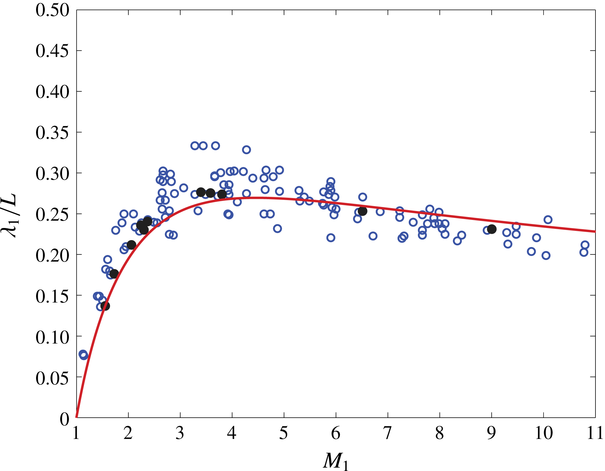
The shock structure based on the Navier–Stokes–Fourier (NSF) equations has been well characterized (Morduchow & Libby Reference Morduchow and Libby1949; von Mises Reference von Mises1950; Gilbarg Reference Gilbarg1951; Ludford Reference Ludford1951; Gilbarg & Paolucci Reference Gilbarg and Paolucci1953; Khonkin & Orlov Reference Khonkin and Orlov1993). In addition, a number of experimental studies have provided measurements of the shock structure over varying Mach number ranges (Sherman Reference Sherman1955; Linzer & Hornig Reference Linzer and Hornig1963; Camac Reference Camac and de Leeuw1965; Russell Reference Russell1965; Schultz-Grunow & Frohn Reference Schultz-Grunow, Frohn and de Leeuw1965; Robben & Talbot Reference Robben and Talbot1966; Schmidt Reference Schmidt1969; Rieutord Reference Rieutord1970; Garen, Synofzik & Frohn Reference Garen, Synofzik and Frohn1974). In particular, accurate density measurements have been carried out in argon and nitrogen shock waves for a large Mach number range by Alsmeyer (Reference Alsmeyer1976). Subsequently, it is well known that the NSF equations do not represent the shock structure well even at moderate Mach numbers (see Gilbarg & Paolucci Reference Gilbarg and Paolucci1953; Liepmann, Narasimha & Chahine Reference Liepmann, Narasimha and Chahine1962; Alsmeyer Reference Alsmeyer1976); the shock layer thickness is predicted to be too small compared to experiments, particularly at intermediate Mach numbers. In figure 1 the inverse shock thickness as a function of the upstream Mach number predicted by the NSF theory (and by a number of other theories discussed below) is compared with experimental results (open circles). As can be observed, values obtained from the NSF equations differ significantly from the experimental measurements for Mach numbers larger than approximately 1.5.

Figure 1.

Inverse shock thickness, $\unicode[STIX]{x1D706}_{1}/L$ , as a function of upstream Mach number, $M_{1}$ , for argon gas: ○, experimental results of Linzer & Hornig (Reference Linzer and Hornig1963), Camac (Reference Camac and de Leeuw1965), Russell (Reference Russell1965), Schultz-Grunow & Frohn (Reference Schultz-Grunow, Frohn and de Leeuw1965), Robben & Talbot (Reference Robben and Talbot1966), Schmidt (Reference Schmidt1969), Rieutord (Reference Rieutord1970), Garen et al. (Reference Garen, Synofzik and Frohn1974) and Alsmeyer (Reference Alsmeyer1976); – – –, NSF theory;

, direct simulation Monte Carlo results of Bird (1970); ——, theoretical results of Lumpkin & Chapman (1992), Woods (1993) and Reese et al. (1995).

The NSF equations represent a continuum theory based on linear constitutive relations between thermodynamic forces and fluxes (note that in general the Stokes assumption regarding bulk viscosity is not assumed). In a strong shock wave, the forces are large and the failure of the NSF equations could be attributed to deviations from the linear Newtonian and Fourier laws or to a mean free path too large for the continuum assumption to be accurate. Subsequently, the computation of the shock structure, particularly at the large Mach numbers encountered in hypersonic flows, has provided an excellent opportunity to find extended theories that would remedy this discrepancy.

The generally accepted parameter which indicates the extent to which a local region of flowing gas is in thermodynamic equilibrium is the Knudsen number, $Kn=\unicode[STIX]{x1D706}/L\propto M/Re$ , where $\unicode[STIX]{x1D706}$ is the mean free path of the gas molecules, $L$ is a characteristic length of the flow system, $M=u/c$ is the flow Mach number with $u$ the flow speed and $c$ the speed of sound and $Re=\unicode[STIX]{x1D70C}\,u\,L/\unicode[STIX]{x1D707}$ is the Reynolds number with $\unicode[STIX]{x1D70C}$ the mass density and $\unicode[STIX]{x1D707}$ the dynamic viscosity. If $Kn$ is less than $10^{-3}$ , the gas can be assumed to undergo a large number of collisions over the typical length scale, and the conventional NSF equations are an appropriate model. Difficulties appear when $Kn$ rises, either due to the low density of the gas (which makes the mean free path larger) or due to regions of high local gradients, such as in the shock structure. The situation becomes even more problematic as $Kn$ rises to the range 0.1–1. This is called the ‘transition–continuum regime’ and it lies between the extremes of the continuum and free molecular regimes. The range of use of the continuum–equilibrium assumption is therefore clearly limited, with the applicability of the classical NSF equations (with standard no-slip boundary conditions) confined to cases where $Kn\lesssim 0.01$ , typically. The flow in the shock layer is far from being in local thermodynamic equilibrium, typically $Kn=0.2$ –0.3, i.e. very much within the intermediate- $Kn$ regime.

Extended, or modified, hydrodynamics attempts to increase the range of applicability of the continuum–equilibrium fluid model into the transition–continuum regime where $0.01\lesssim Kn\lesssim 1$ . Since the NSF equations perform poorly at these values of $Kn$ , the shock structure problem is particularly well suited for testing extended hydrodynamic models. (In passing, it should be noted that the linear NSF theory has been extended in liquids when dealing with what we call viscoelastic materials.)

Numerous higher-order continuum-fluid equation sets have been proposed for flows that depart from quasi thermodynamic equilibrium, mostly derived from the fundamental Boltzmann equation using different approaches (Thomas Reference Thomas1944; Liepmann et al. Reference Liepmann, Narasimha and Chahine1962). In its most basic form, the Boltzmann equation describes the evolution of a system of monatomic gas molecules, assuming molecular chaos and that only binary inter-molecular collisions occur (i.e. the gas needs to be dilute, although there are potential modifications which could allow for multiple collisions typical of dense gases). All such theories discussed below are limited to monatomic gases. The classical approach is the Chapman–Enskog technique (based on a series expansion in $Kn$ ) which determines a hierarchy of approximate solutions to the Boltzmann equation. The approach is limited by the convergence of the series ( $Kn\lesssim 0.3$ ). The first term in the series results in the stress tensor equal to the pressure and the heat flux being zero (Euler equations). The first two terms in the series result in the linear constitutive equations associated with the NSF equations. The first three terms (second order in $Kn$ ) provide a complicated set of constitutive equations known as the Burnett equations (Chapman & Cowling Reference Chapman and Cowling1970), which are presumed to extend the validity of the continuum model for flows at higher $Kn$ than the NSF equations. Other similar second-order formulations include Grad’s 13 moment (Grad Reference Grad1949, Reference Grad1952), reduced Burnett (Lumpkin & Chapman Reference Lumpkin and Chapman1992), BGK-Burnett (Bhatnagar–Gross–Krook/Burnett) (Balakrishnan Reference Balakrishnan2004), regularized Burnett and regularized Grad’s 13 moment (Jin & Slemrod Reference Jin and Slemrod2001; Struchtrup & Torrilhon Reference Struchtrup and Torrilhon2003) and Woods (Woods Reference Woods1983, Reference Woods1993; Reese et al. Reference Reese, Woods, Thivet and Candel1995) equations. This is not an exhaustive list, but includes the most commonly used and cited. Balakrishnan & Agarwal (Reference Balakrishnan and Agarwal1999) provide a comparative study of second-order kinetic formulations applied to the shock structure problem. Most of these theories amount to adding, removing or modifying in an ad hoc fashion different terms in the Burnett equations or variants thereof. The leading reason for such modifications is that they are all plagued by numerical and physical instabilities and, in many cases, produce non-physical flow predictions. For example, Grad’s 13-moment theory provides no continuous shock structure beyond $M=1.65$ . Similar to Grad’s theory of moments, Weiss and others (Liu & Salvador Reference Liu and Salvador1990; Weiss Reference Weiss1995; Taniguchi et al. Reference Taniguchi, Arima, Ruggeri and Sujiyama2014a ,Reference Taniguchi, Arima, Ruggeri and Sujiyama b ) extend the theory from 13 to 21 moments for densities of momentum and energy fluxes. Depending on the number of moments, there is a critical Mach number beyond which there are no solutions. The critical Mach number depends on the number of moments; it is 1.65 for 13 moments and 1.887 for 21 moments. We note that the result shown in figure 1 corresponds to that of Reese et al. (Reference Reese, Woods, Thivet and Candel1995) obtained by ad hoc alteration and deletion of terms giving rise to non-physical effects in modified Barnett equations. The explanation of problems with stability may have been provided by Comeaux, Chapman & MacCormack (Reference Comeaux, Chapman and MacCormack1995) who showed that the Burnett equations can violate the second law of thermodynamics.

Direct simulation Monte Carlo (DSMC) and molecular dynamics (MD) have also been used to obtain the shock structure (Bird Reference Bird1970; Salomons & Mareschal Reference Salomons and Mareschal1992). As shown in figure 1, the DSMC results, obtained by using a simple repulsive intermolecular force law, show very good agreement with the experimental results over the large Mach number range. However, the large number of molecules required to accurately simulate the continuum–transition regime makes the DSMC technique prohibitively expensive with regard to computational cost and limits its applicability to simulations of flows in simple geometries.

It is noted that there have been extensions to the NSF theory in a variety of directions. In kinetic theory, there are works that consider polyatomic gases (Brau Reference Brau1967; She & Sather Reference She and Sather1967). In continuum theory, the most prominent extensions have been in the area of non-Newtonian and viscoelastic fluids (Coleman & Noll Reference Coleman and Noll1961; Coleman, Markovitz & Noll Reference Coleman, Markovitz and Noll1966). There have also been many works that consider fluids that can sustain internal spin under the rubric of micropolar or couple stress, but they all fall under the general micromorphic theory of Eringen (Reference Eringen1999, Reference Eringen2001). A noteworthy extension is also that of Chen (Reference Chen2013) where the rate of temperature is accounted for in the formulation of the constitutive theory. Lastly, we note that Brenner (Reference Brenner2005a ,Reference Brenner b ) proposed modifications of the NSF equations based on a diffusion of volume argument which would be significant for flows with large density gradients. Greenshields & Reese (Reference Greenshields and Reese2007) modified Brenner’s equations by introducing an additional physical parameter, the volume diffusivity. They applied their modified equations to the solutions of the steady shock wave as a test, and computed the structure in the Mach number range of 1–12. They also encountered instabilities in the solutions. Nevertheless, they were able to ‘adjust’ the equations to obtain somewhat better solutions than NSF equations with the addition of two terms.

In this work we use standard continuum theory to extend the constitutive equations. In § 2 we write the governing continuum balance equations for mass, linear momentum and energy, along with the entropy inequality representing the second law of thermodynamics. In § 3 we extend the constitutive equations necessitated by these equations to second order, not in Knudsen number, but in strain rate and gradients of density and temperature. We also discuss related equations of state. In § 4 we write the one-dimensional form of the governing equations relevant to the shock structure problem. The results for argon and nitrogen are presented in § 5. In § 6 we compare the new constitutive equations with those obtained through the Chapman–Enskog expansion and discuss the advantages of the extended model derived in the present work.

2 Governing equations

Ignoring external sources of momentum and energy, and assuming sufficient material smoothness, the fundamental local laws of conservation of mass, linear momentum and energy are given by

(2.1)

$$\begin{eqnarray}\displaystyle & \displaystyle \dot{\unicode[STIX]{x1D70C}}+\unicode[STIX]{x1D70C}\,\text{div}\,\boldsymbol{v}=0, & \displaystyle\end{eqnarray}$$

(2.2)

$$\begin{eqnarray}\displaystyle & \displaystyle \unicode[STIX]{x1D70C}\,\dot{\boldsymbol{v}}-\text{div}\,\unicode[STIX]{x1D748}=\mathbf{0}, & \displaystyle\end{eqnarray}$$

(2.3)

$$\begin{eqnarray}\displaystyle & \displaystyle \unicode[STIX]{x1D70C}\,{\dot{e}}-\unicode[STIX]{x1D6F7}+\text{div}\,\boldsymbol{q}=0, & \displaystyle\end{eqnarray}$$

where a superposed dot denotes the material derivative,

(2.4)

$$\begin{eqnarray}\displaystyle {\dot{f}}=\frac{\unicode[STIX]{x2202}f}{\unicode[STIX]{x2202}t}+\boldsymbol{v}\boldsymbol{\cdot }\text{grad}\,f, & & \displaystyle\end{eqnarray}$$

and ‘ $\text{grad}$ ’ and ‘ $\text{div}$ ’ denote the gradient and divergence operators. It is known that in addition to the above equations, the local form of the entropy inequality,

(2.5)

$$\begin{eqnarray}\displaystyle \unicode[STIX]{x1D6FE}_{v}=\unicode[STIX]{x1D70C}\,\dot{\unicode[STIX]{x1D702}}+\text{div}\,\boldsymbol{h}\geqslant 0, & & \displaystyle\end{eqnarray}$$

must be satisfied. In the above equations, $\unicode[STIX]{x1D70C}>0$ is the mass density, $\boldsymbol{v}$ the velocity, $e$ the internal energy density, $\unicode[STIX]{x1D702}$ the entropy density, $\unicode[STIX]{x1D6FE}_{v}$ the entropy production density, $\unicode[STIX]{x1D6F7}=\boldsymbol{D}\boldsymbol{ : }\unicode[STIX]{x1D748}$ the mechanical energy (or stress power) with $\boldsymbol{D}=\text{sym}\,(\text{grad}\,\boldsymbol{v})$ (‘ $\text{sym}$ ’ denotes the symmetric part), $\unicode[STIX]{x1D748}$ is the symmetric Cauchy stress tensor (the symmetry requirement arises from the balance of angular momentum), $\boldsymbol{q}$ the heat flux and $\boldsymbol{h}$ the entropy flux.

3 Constitutive equations

We note that the entropy inequality (2.5), using the energy conservation (2.3), can be rewritten in terms of the Helmholtz free energy density $\unicode[STIX]{x1D713}=e-\unicode[STIX]{x1D703}\,\unicode[STIX]{x1D702}$ :

(3.1)

$$\begin{eqnarray}\displaystyle \unicode[STIX]{x1D6FE}_{v}\,\unicode[STIX]{x1D703}=-\unicode[STIX]{x1D70C}(\dot{\unicode[STIX]{x1D713}}+\unicode[STIX]{x1D702}\,\dot{\unicode[STIX]{x1D703}})+\unicode[STIX]{x1D63F}\boldsymbol{ : }\unicode[STIX]{x1D748}-\frac{\boldsymbol{q}}{\unicode[STIX]{x1D703}}\boldsymbol{\cdot }\boldsymbol{g}+\unicode[STIX]{x1D703}\,\text{div}\,\boldsymbol{k}\geqslant 0, & & \displaystyle\end{eqnarray}$$

where $\boldsymbol{g}\equiv \text{grad}\,\unicode[STIX]{x1D703}$ and

(3.2)

$$\begin{eqnarray}\displaystyle \boldsymbol{k}\equiv \boldsymbol{h}-\frac{\boldsymbol{q}}{\unicode[STIX]{x1D703}} & & \displaystyle\end{eqnarray}$$

is the extra entropy flux. We take the constitutive quantities to be given by

(3.3)

$$\begin{eqnarray}\displaystyle {\mathcal{C}}=\{\unicode[STIX]{x1D713},\unicode[STIX]{x1D702},\boldsymbol{q},\boldsymbol{k},\unicode[STIX]{x1D748}\} & & \displaystyle\end{eqnarray}$$

and which, utilizing frame invariance, for a fluid are functions of the independent basic fields

(3.4)

$$\begin{eqnarray}\displaystyle {\mathcal{I}}=\{\unicode[STIX]{x1D70C},\boldsymbol{r},\unicode[STIX]{x1D63F},\unicode[STIX]{x1D703},\boldsymbol{g}\}, & & \displaystyle\end{eqnarray}$$

where $\unicode[STIX]{x1D703}>0$ is the absolute temperature and $\boldsymbol{r}\equiv \text{grad}\,\unicode[STIX]{x1D70C}$ . This material corresponds to a non-simple (isotropic) fluid.

Using (3.1), it can be subsequently shown that (see appendix A)

(3.5)

$$\begin{eqnarray}\displaystyle & \displaystyle \unicode[STIX]{x1D713}=\unicode[STIX]{x1D713}(\unicode[STIX]{x1D70C},\unicode[STIX]{x1D703}), & \displaystyle\end{eqnarray}$$

(3.6)

$$\begin{eqnarray}\displaystyle & \displaystyle \unicode[STIX]{x1D702}=-\frac{\unicode[STIX]{x2202}\unicode[STIX]{x1D713}}{\unicode[STIX]{x2202}\unicode[STIX]{x1D703}}, & \displaystyle\end{eqnarray}$$

and $\boldsymbol{k}=\mathbf{0}$ , or

(3.7)

$$\begin{eqnarray}\displaystyle \boldsymbol{h}=\frac{\boldsymbol{q}}{\unicode[STIX]{x1D703}}. & & \displaystyle\end{eqnarray}$$

Furthermore, in conjunction with (2.2) and (2.3), and the thermodynamic static equilibrium stability conditions (where $\unicode[STIX]{x1D6FE}_{v}=0$ when $\boldsymbol{r}=\mathbf{0}$ , $\boldsymbol{g}=\mathbf{0}$ , and $\unicode[STIX]{x1D63F}=\mathbf{0}$ ; we assume that the constitutive quantities in (3.3) have continuous second derivatives with respect to the independent basic fields in (3.4) at equilibrium), we conclude that

(3.8)

$$\begin{eqnarray}\displaystyle & \displaystyle \boldsymbol{q}=\boldsymbol{q}^{d}(\unicode[STIX]{x1D70C},\boldsymbol{r},\unicode[STIX]{x1D63F},\unicode[STIX]{x1D703},\boldsymbol{g}), & \displaystyle\end{eqnarray}$$

(3.9)

$$\begin{eqnarray}\displaystyle & \displaystyle \unicode[STIX]{x1D748}=-p\,\mathbf{1}+\unicode[STIX]{x1D748}^{d}(\unicode[STIX]{x1D70C},\boldsymbol{r},\unicode[STIX]{x1D63F},\unicode[STIX]{x1D703},\boldsymbol{g}), & \displaystyle\end{eqnarray}$$

where $\mathbf{1}$ is the unit tensor and

(3.10)

$$\begin{eqnarray}\displaystyle p=\unicode[STIX]{x1D70C}^{2}\,\frac{\unicode[STIX]{x2202}\unicode[STIX]{x1D713}}{\unicode[STIX]{x2202}\unicode[STIX]{x1D70C}} & & \displaystyle\end{eqnarray}$$

is the thermodynamic pressure. From the above definition of a thermodynamic equilibrium state, we note that $\unicode[STIX]{x1D748}^{d}$ and $\boldsymbol{q}^{d}$ must vanish when $\boldsymbol{r}$ , $\boldsymbol{g}$ and $\unicode[STIX]{x1D63F}$ vanish. In addition, using (3.8)–(3.10), the reduced entropy inequality (A 28) becomes

(3.11)

$$\begin{eqnarray}\displaystyle \unicode[STIX]{x1D6FE}_{v}\,\unicode[STIX]{x1D703}=\unicode[STIX]{x1D748}^{d}\boldsymbol{ : }\unicode[STIX]{x1D63F}-\frac{\boldsymbol{q}^{d}}{\unicode[STIX]{x1D703}}\boldsymbol{\cdot }\boldsymbol{g}\geqslant 0. & & \displaystyle\end{eqnarray}$$

This inequality shows that heat, in the presence of deformation, does not, in general, flow from higher to lower temperatures.

From Paolucci (Reference Paolucci2016, tables 5.1–5.3) (see also Eringen (Reference Eringen1980), Zheng (Reference Zheng1993, Reference Zheng1994) and Liu (Reference Liu2002)) we can immediately write down the representations of $q_{i}^{d}$ and $\unicode[STIX]{x1D70E}_{ik}^{d}$ corresponding to isotropic vector-valued and symmetric tensor-valued functions of vectors $g_{i}=\unicode[STIX]{x1D703}_{,i}$ and $r_{i}=\unicode[STIX]{x1D70C}_{,i}$ and symmetric second-order tensor $\unicode[STIX]{x1D60B}_{ik}$ :

(3.12)

$$\begin{eqnarray}\displaystyle q_{i}^{d} & = & \displaystyle -(\unicode[STIX]{x1D705}_{0}\,\unicode[STIX]{x1D6FF}_{il}+\unicode[STIX]{x1D705}_{1}\,\unicode[STIX]{x1D60B}_{il}+\unicode[STIX]{x1D705}_{2}\,\unicode[STIX]{x1D60B}_{ik}\unicode[STIX]{x1D60B}_{kl})\unicode[STIX]{x1D703}_{,l}-(\unicode[STIX]{x1D705}_{3}\,\unicode[STIX]{x1D6FF}_{il}+\unicode[STIX]{x1D705}_{4}\,\unicode[STIX]{x1D60B}_{il}+\unicode[STIX]{x1D705}_{5}\,\unicode[STIX]{x1D60B}_{ik}\unicode[STIX]{x1D60B}_{kl})\unicode[STIX]{x1D70C}_{,l},\end{eqnarray}$$

(3.13)

$$\begin{eqnarray}\displaystyle \unicode[STIX]{x1D70E}_{ik}^{d} & = & \displaystyle \unicode[STIX]{x1D6FC}_{0}\,\unicode[STIX]{x1D6FF}_{ik}+\unicode[STIX]{x1D6FC}_{1}\,\unicode[STIX]{x1D60B}_{ik}+\unicode[STIX]{x1D6FC}_{2}\,\unicode[STIX]{x1D60B}_{il}\unicode[STIX]{x1D60B}_{lk}+\unicode[STIX]{x1D6FC}_{3}\,\unicode[STIX]{x1D703}_{,i}\unicode[STIX]{x1D703}_{,k}+{\textstyle \frac{1}{2}}\,\unicode[STIX]{x1D6FC}_{4}\,(\unicode[STIX]{x1D703}_{,i}\unicode[STIX]{x1D60B}_{kl}+\unicode[STIX]{x1D703}_{,k}\unicode[STIX]{x1D60B}_{il})\unicode[STIX]{x1D703}_{,l}\nonumber\\ \displaystyle & & \displaystyle +\,{\textstyle \frac{1}{2}}\,\unicode[STIX]{x1D6FC}_{5}\,(\unicode[STIX]{x1D703}_{,i}\unicode[STIX]{x1D60B}_{kl}+\unicode[STIX]{x1D703}_{,k}\unicode[STIX]{x1D60B}_{il})\unicode[STIX]{x1D60B}_{lm}\unicode[STIX]{x1D703}_{,m}+\unicode[STIX]{x1D6FC}_{6}\,\unicode[STIX]{x1D70C}_{,i}\unicode[STIX]{x1D70C}_{,k}+{\textstyle \frac{1}{2}}\unicode[STIX]{x1D6FC}_{7}\,(\unicode[STIX]{x1D70C}_{,i}\unicode[STIX]{x1D60B}_{kl}+\unicode[STIX]{x1D70C}_{,k}\unicode[STIX]{x1D60B}_{il})\unicode[STIX]{x1D70C}_{,l}\nonumber\\ \displaystyle & & \displaystyle +\,{\textstyle \frac{1}{2}}\,\unicode[STIX]{x1D6FC}_{8}\,(\unicode[STIX]{x1D70C}_{,i}\unicode[STIX]{x1D60B}_{kl}+\unicode[STIX]{x1D70C}_{,k}\unicode[STIX]{x1D60B}_{il})\unicode[STIX]{x1D60B}_{lm}\unicode[STIX]{x1D70C}_{,m}+{\textstyle \frac{1}{2}}\,\unicode[STIX]{x1D6FC}_{9}\,(\unicode[STIX]{x1D703}_{,i}\unicode[STIX]{x1D70C}_{,k}+\unicode[STIX]{x1D70C}_{,i}\unicode[STIX]{x1D703}_{,k})\nonumber\\ \displaystyle & & \displaystyle +\,{\textstyle \frac{1}{2}}\,\unicode[STIX]{x1D6FC}_{10}[\unicode[STIX]{x1D60B}_{il}(\unicode[STIX]{x1D70C}_{,l}\unicode[STIX]{x1D703}_{,k}-\unicode[STIX]{x1D703}_{,l}\unicode[STIX]{x1D70C}_{,k})-(\unicode[STIX]{x1D70C}_{,i}\unicode[STIX]{x1D703}_{,l}-\unicode[STIX]{x1D703}_{,i}\unicode[STIX]{x1D70C}_{,l})\unicode[STIX]{x1D60B}_{kl}],\end{eqnarray}$$

where $\unicode[STIX]{x1D705}_{p}$ ( $p=0,\ldots ,5$ ) and $\unicode[STIX]{x1D6FC}_{q}$ ( $q=0,\ldots ,10$ ) are functions of $\unicode[STIX]{x1D70C}$ , $\unicode[STIX]{x1D703}$ and the isotropic scalar invariants $\{I_{1},\ldots ,I_{12}\}$ , where

(3.14)

$$\begin{eqnarray}\displaystyle & \displaystyle I_{1}=\unicode[STIX]{x1D60B}_{ii}=D_{(1)}, & \displaystyle\end{eqnarray}$$

(3.15)

$$\begin{eqnarray}\displaystyle & \displaystyle I_{2}=\unicode[STIX]{x1D60B}_{ik}\unicode[STIX]{x1D60B}_{ki}=D_{(1)}^{2}-2D_{(2)}, & \displaystyle\end{eqnarray}$$

(3.16)

$$\begin{eqnarray}\displaystyle & \displaystyle I_{3}=\unicode[STIX]{x1D60B}_{ik}\unicode[STIX]{x1D60B}_{kl}\unicode[STIX]{x1D60B}_{li}=D_{(1)}^{3}-3D_{(1)}D_{(2)}+3D_{(3)}, & \displaystyle\end{eqnarray}$$

(3.17a-c )

$$\begin{eqnarray}\displaystyle I_{4}=\unicode[STIX]{x1D703}_{,i}\unicode[STIX]{x1D703}_{,i},\quad I_{5}=\unicode[STIX]{x1D703}_{,i}\unicode[STIX]{x1D60B}_{ik}\unicode[STIX]{x1D703}_{,k},\quad I_{6}=\unicode[STIX]{x1D703}_{,i}\unicode[STIX]{x1D60B}_{ik}\unicode[STIX]{x1D60B}_{kl}\unicode[STIX]{x1D703}_{,l}, & & \displaystyle\end{eqnarray}$$

(3.18a-c )

$$\begin{eqnarray}\displaystyle I_{7}=\unicode[STIX]{x1D70C}_{,i}\unicode[STIX]{x1D70C}_{,i},\quad I_{8}=\unicode[STIX]{x1D70C}_{,i}\unicode[STIX]{x1D60B}_{ik}\unicode[STIX]{x1D70C}_{,k},\quad I_{9}=\unicode[STIX]{x1D70C}_{,i}\unicode[STIX]{x1D60B}_{ik}\unicode[STIX]{x1D60B}_{kl}\unicode[STIX]{x1D70C}_{,l}, & & \displaystyle\end{eqnarray}$$

(3.19a-c )

$$\begin{eqnarray}\displaystyle I_{10}=\unicode[STIX]{x1D70C}_{,i}\unicode[STIX]{x1D703}_{,i},\quad I_{11}=\unicode[STIX]{x1D70C}_{,i}\unicode[STIX]{x1D60B}_{ik}\unicode[STIX]{x1D703}_{,k},\quad I_{12}=\unicode[STIX]{x1D70C}_{,i}\unicode[STIX]{x1D60B}_{ik}\unicode[STIX]{x1D60B}_{kl}\unicode[STIX]{x1D703}_{,l}, & & \displaystyle\end{eqnarray}$$

and

(3.20a-c )

$$\begin{eqnarray}\displaystyle D_{(1)}=d^{(1)}+d^{(2)}+d^{(3)},\quad D_{(2)}=d^{(1)}d^{(2)}+d^{(2)}d^{(3)}+d^{(3)}d^{(1)},\quad D_{(3)}=d^{(1)}d^{(2)}d^{(3)}, & & \displaystyle \nonumber\\ \displaystyle & & \displaystyle\end{eqnarray}$$

where $D_{(i)}$ and $d^{(i)}$ , $i=1,2,3$ , are the invariants and the principal deformation rates of $\unicode[STIX]{x1D60B}_{ik}$ , respectively. In the representation (3.13), we require that $\unicode[STIX]{x1D6FC}_{0}\rightarrow 0$ as $\unicode[STIX]{x1D70C}_{,i}\rightarrow 0$ , $\unicode[STIX]{x1D703}_{,i}\rightarrow 0$ and $\unicode[STIX]{x1D60B}_{ik}\rightarrow 0$ , since as we approach equilibrium, we must have $\unicode[STIX]{x1D70E}_{ik}^{d}\rightarrow 0$ .

Now, substituting the representations (3.12) and (3.13) into the reduced entropy inequality (3.11), and using the Cayley–Hamilton theorem and the definitions of the invariants (3.14)–(3.19), we obtain

(3.21)

$$\begin{eqnarray}\displaystyle 0\leqslant \unicode[STIX]{x1D6FE}_{v}\,\unicode[STIX]{x1D703} & = & \displaystyle \unicode[STIX]{x1D6FC}_{0}I_{1}+\unicode[STIX]{x1D6FC}_{1}I_{2}+\unicode[STIX]{x1D6FC}_{2}I_{3}+\left[\frac{1}{6}\unicode[STIX]{x1D6FC}_{5}(I_{1}^{3}-3I_{1}I_{2}+2I_{3})+\frac{\unicode[STIX]{x1D705}_{0}}{\unicode[STIX]{x1D703}}\right]I_{4}\nonumber\\ \displaystyle & & \displaystyle +\left[\unicode[STIX]{x1D6FC}_{3}-\frac{1}{2}\unicode[STIX]{x1D6FC}_{5}(I_{1}^{2}-I_{2})+\frac{\unicode[STIX]{x1D705}_{1}}{\unicode[STIX]{x1D703}}\right]I_{5}+\left(\unicode[STIX]{x1D6FC}_{4}+\unicode[STIX]{x1D6FC}_{5}I_{1}+\frac{\unicode[STIX]{x1D705}_{2}}{\unicode[STIX]{x1D703}}\right)I_{6}\nonumber\\ \displaystyle & & \displaystyle +\,\frac{1}{6}\unicode[STIX]{x1D6FC}_{8}(I_{1}^{3}-3I_{1}I_{2}+2I_{3})I_{7}+\left[\unicode[STIX]{x1D6FC}_{6}-\frac{1}{2}\unicode[STIX]{x1D6FC}_{8}(I_{1}^{2}-I_{2})\right]I_{8}\nonumber\\ \displaystyle & & \displaystyle +\,(\unicode[STIX]{x1D6FC}_{7}+\unicode[STIX]{x1D6FC}_{8}I_{1})I_{9}+\frac{\unicode[STIX]{x1D705}_{3}}{\unicode[STIX]{x1D703}}\,I_{10}+\left(\unicode[STIX]{x1D6FC}_{9}+\frac{\unicode[STIX]{x1D705}_{4}}{\unicode[STIX]{x1D703}}\right)I_{11}+\frac{\unicode[STIX]{x1D705}_{5}}{\unicode[STIX]{x1D703}}\,I_{12}\end{eqnarray}$$

(3.22)

$$\begin{eqnarray}\displaystyle & = & \displaystyle \unicode[STIX]{x1D6FC}_{0}D_{(1)}+\unicode[STIX]{x1D6FC}_{1}(D_{(1)}^{2}-2D_{(2)})+\unicode[STIX]{x1D6FC}_{2}(D_{(1)}^{3}-3D_{(1)}D_{(2)}+3D_{(3)})\nonumber\\ \displaystyle & & \displaystyle +\left(\unicode[STIX]{x1D6FC}_{5}D_{(3)}+\frac{\unicode[STIX]{x1D705}_{0}}{\unicode[STIX]{x1D703}}\right)I_{4}+\left(\unicode[STIX]{x1D6FC}_{3}-\unicode[STIX]{x1D6FC}_{5}D_{(2)}+\frac{\unicode[STIX]{x1D705}_{1}}{\unicode[STIX]{x1D703}}\right)I_{5}+\left(\unicode[STIX]{x1D6FC}_{4}+\unicode[STIX]{x1D6FC}_{5}D_{(1)}+\frac{\unicode[STIX]{x1D705}_{2}}{\unicode[STIX]{x1D703}}\right)I_{6}\nonumber\\ \displaystyle & & \displaystyle +\,\unicode[STIX]{x1D6FC}_{8}D_{(3)}I_{7}+(\unicode[STIX]{x1D6FC}_{6}-\unicode[STIX]{x1D6FC}_{8}D_{(2)})I_{8}+(\unicode[STIX]{x1D6FC}_{7}+\unicode[STIX]{x1D6FC}_{8}D_{(1)})I_{9}+\frac{\unicode[STIX]{x1D705}_{3}}{\unicode[STIX]{x1D703}}\,I_{10}\nonumber\\ \displaystyle & & \displaystyle +\left(\unicode[STIX]{x1D6FC}_{9}+\frac{\unicode[STIX]{x1D705}_{4}}{\unicode[STIX]{x1D703}}\right)I_{11}+\frac{\unicode[STIX]{x1D705}_{5}}{\unicode[STIX]{x1D703}}\,I_{12}.\end{eqnarray}$$

The constitutive equations (3.12) and (3.13) are too complicated for solutions of fluid problems. Generally, polynomial approximations of various degrees (denoted by ‘deg’) in $\boldsymbol{D}$ , $\boldsymbol{r}$ , and $\boldsymbol{g}$ are used. We note that $\text{deg}\,I_{1}=\text{deg}\,D_{(1)}=1$ , $\text{deg}\,I_{2}=\text{deg}\,D_{(2)}=2$ , $\text{deg}\,I_{3}=\text{deg}\,D_{(3)}=3$ , $\text{deg}\,I_{4}=2$ , $\text{deg}\,I_{5}=3$ , $\text{deg}\,I_{6}=4$ , $\text{deg}\,I_{7}=2$ , $\text{deg}\,I_{8}=3$ , $\text{deg}\,I_{9}=4$ , $\text{deg}\,I_{10}=2$ , $\text{deg}\,I_{11}=3$ and $\text{deg}\,I_{12}=4$ . Subsequently, for $q_{i}^{d}$ to be of order $N$ , $\unicode[STIX]{x1D705}_{0}$ and $\unicode[STIX]{x1D705}_{3}$ , $\unicode[STIX]{x1D705}_{1}$ and $\unicode[STIX]{x1D705}_{4}$ and $\unicode[STIX]{x1D705}_{2}$ and $\unicode[STIX]{x1D705}_{5}$ , can at most be of degrees $N-1$ , $N-2$ and $N-3$ , respectively, while for $\unicode[STIX]{x1D70E}_{ik}^{d}$ to be of order $N$ , $\unicode[STIX]{x1D6FC}_{0}$ , $\unicode[STIX]{x1D6FC}_{1}$ , $\unicode[STIX]{x1D6FC}_{2}$ , $\unicode[STIX]{x1D6FC}_{3}$ , $\unicode[STIX]{x1D6FC}_{4}$ , $\unicode[STIX]{x1D6FC}_{5}$ , $\unicode[STIX]{x1D6FC}_{6}$ , $\unicode[STIX]{x1D6FC}_{7}$ , $\unicode[STIX]{x1D6FC}_{8}$ , $\unicode[STIX]{x1D6FC}_{9}$ and $\unicode[STIX]{x1D6FC}_{10}$ can at most be of degrees $N$ , $N-1$ , $N-2$ , $N-2$ , $N-3$ , $N-4$ , $N-2$ , $N-3$ , $N-4$ , $N-2$ and $N-3$ , respectively.

Second-order representations

If we write second-order expansions of (3.12) and (3.13) (i.e. we take $N=2$ ) in the limits $\unicode[STIX]{x1D70C}_{,i}\rightarrow 0$ , $\unicode[STIX]{x1D703}_{,i}\rightarrow 0$ and $\unicode[STIX]{x1D60B}_{ik}\rightarrow 0$ , we require that $\unicode[STIX]{x1D705}_{0}=k_{00}+k_{01}D_{(1)}$ , $\unicode[STIX]{x1D705}_{1}=k_{10}$ , $\unicode[STIX]{x1D705}_{2}=0$ , $\unicode[STIX]{x1D705}_{3}=k_{30}+k_{31}D_{(1)}$ , $\unicode[STIX]{x1D705}_{4}=k_{40}$ , $\unicode[STIX]{x1D705}_{5}=0$ , $\unicode[STIX]{x1D6FC}_{0}=a_{0000}+a_{0100}D_{(1)}+a_{0200}D_{(1)}^{2}+a_{0010}D_{(2)}+a_{0001}I_{4}+a_{0002}I_{7}+a_{0003}I_{10}$ , $\unicode[STIX]{x1D6FC}_{1}=a_{10}+a_{11}D_{(1)}$ , $\unicode[STIX]{x1D6FC}_{2}=a_{20}$ , $\unicode[STIX]{x1D6FC}_{3}=a_{30}$ , $\unicode[STIX]{x1D6FC}_{4}=\unicode[STIX]{x1D6FC}_{5}=0$ , $\unicode[STIX]{x1D6FC}_{6}=a_{60}$ , $\unicode[STIX]{x1D6FC}_{7}=\unicode[STIX]{x1D6FC}_{8}=0$ , $\unicode[STIX]{x1D6FC}_{9}=a_{90}$ and $\unicode[STIX]{x1D6FC}_{10}=0$ . Note that now $k_{00}$ , $k_{01}$ , $k_{10}$ , $k_{30}$ , $k_{31}$ , $k_{40}$ , $a_{0000}$ , $a_{0100}$ , $a_{0200}$ , $a_{0010}$ , $a_{0001}$ , $a_{0002}$ , $a_{0003}$ , $a_{10}$ , $a_{11}$ , $a_{20}$ , $a_{30}$ and $a_{60}$ are only functions of $\unicode[STIX]{x1D70C}$ and $\unicode[STIX]{x1D703}$ . Subsequently, since $q_{i}^{d}$ and $\unicode[STIX]{x1D60B}_{ik}^{d}$ must vanish as $\unicode[STIX]{x1D70C}_{,i}\rightarrow 0$ , $\unicode[STIX]{x1D703}_{,i}\rightarrow 0$ , and $\unicode[STIX]{x1D60B}_{ik}\rightarrow 0$ , we have that $a_{0000}=0$ and thus

(3.23)

$$\begin{eqnarray}\displaystyle q_{i}^{d} & = & \displaystyle -[(k_{00}+k_{01}D_{(1)})\unicode[STIX]{x1D6FF}_{il}+k_{10}\unicode[STIX]{x1D60B}_{il}]\unicode[STIX]{x1D703}_{,l}-[(k_{30}+k_{31}D_{(1)})\unicode[STIX]{x1D6FF}_{il}+k_{40}\unicode[STIX]{x1D60B}_{il}]\unicode[STIX]{x1D70C}_{,l},\end{eqnarray}$$

(3.24)

$$\begin{eqnarray}\displaystyle \unicode[STIX]{x1D70E}_{ik}^{d} & = & \displaystyle (a_{0100}D_{(1)}+a_{0200}D_{(1)}^{2}+a_{0010}D_{(2)}+a_{0001}I_{4}+a_{0002}I_{7}+a_{0003}I_{10})\unicode[STIX]{x1D6FF}_{ik}\nonumber\\ \displaystyle & & \displaystyle +\,(a_{10}+a_{11}D_{(1)})\unicode[STIX]{x1D60B}_{ik}+a_{20}\unicode[STIX]{x1D60B}_{il}\unicode[STIX]{x1D60B}_{lk}+a_{30}\unicode[STIX]{x1D703}_{,i}\unicode[STIX]{x1D703}_{,k}+a_{60}\unicode[STIX]{x1D70C}_{,i}\unicode[STIX]{x1D70C}_{,k}\nonumber\\ \displaystyle & & \displaystyle +\,{\textstyle \frac{1}{2}}a_{90}(\unicode[STIX]{x1D703}_{,i}\unicode[STIX]{x1D70C}_{,k}+\unicode[STIX]{x1D70C}_{,i}\unicode[STIX]{x1D703}_{,k}).\end{eqnarray}$$

Now, using the fact that

(3.25)

$$\begin{eqnarray}\displaystyle D_{(2)}^{\prime }=-{\textstyle \frac{1}{2}}\,\text{tr}({\unicode[STIX]{x1D63F}^{\prime }}^{2})=-{\textstyle \frac{1}{3}}\,D_{(1)}^{2}+D_{(2)}, & & \displaystyle\end{eqnarray}$$

where $D_{(2)}^{\prime }$ denotes the second invariant of the deviatoric part of $\unicode[STIX]{x1D63F}$ , $\unicode[STIX]{x1D63F}^{\prime }=\unicode[STIX]{x1D63F}-1/3\,D_{(1)}\mathbf{1}$ and ‘ $\text{tr}$ ’ denotes the trace, the residual entropy inequality (3.22) for this order of approximation becomes

(3.26)

$$\begin{eqnarray}\displaystyle \unicode[STIX]{x1D6FE}_{v}\,\unicode[STIX]{x1D703} & = & \displaystyle \left(a_{0100}+\frac{1}{3}\,a_{10}\right)D_{(1)}^{2}-2\,a_{10}D_{(2)}^{\prime }+\left(a_{0200}+\frac{1}{3}\,a_{11}+\frac{1}{3}\,a_{0010}\right)D_{(1)}^{3}\nonumber\\ \displaystyle & & \displaystyle +\,(a_{0010}-2\,a_{11}-3\,a_{20})D_{(1)}D_{(2)}^{\prime }+3\,a_{20}D_{(3)}\nonumber\\ \displaystyle & & \displaystyle +\left[\frac{k_{00}}{\unicode[STIX]{x1D703}}+\left(a_{0001}+\frac{k_{01}}{\unicode[STIX]{x1D703}}\right)D_{(1)}\right]I_{4}+\left(a_{30}+\frac{k_{10}}{\unicode[STIX]{x1D703}}\right)I_{5}+a_{0002}D_{(1)}I_{7}\nonumber\\ \displaystyle & & \displaystyle +\,a_{60}I_{8}+\left[\frac{k_{30}}{\unicode[STIX]{x1D703}}+\left(a_{0003}+\frac{k_{31}}{\unicode[STIX]{x1D703}}\right)D_{(1)}\right]I_{10}+\left(a_{90}+\frac{k_{40}}{\unicode[STIX]{x1D703}}\right)I_{11}\geqslant 0.\end{eqnarray}$$

We now examine the restrictions imposed by the reduced entropy inequality (3.26) on the coefficients in (3.23) and (3.24). The inequality must be satisfied for any $\unicode[STIX]{x1D60B}_{ik}$ and any $\unicode[STIX]{x1D70C}_{,i}$ and $\unicode[STIX]{x1D703}_{,i}$ . Specifically, it must be satisfied for any of the following cases.

(1) Consider the case of a stagnant layer of fluid. In this case $\unicode[STIX]{x1D63F}=\mathbf{0}$ , and the reduced entropy inequality (3.26) becomes
(3.27) $$\begin{eqnarray}\displaystyle \frac{k_{00}}{\unicode[STIX]{x1D703}}\,I_{4}+\frac{k_{30}}{\unicode[STIX]{x1D703}}\,I_{10}\geqslant 0. & & \displaystyle\end{eqnarray}$$
Since $I_{4}\geqslant 0$ and $I_{10}$ can be of either sign depending on the signs of the density and temperature gradients, for the inequality to be always satisfied we must have that
(3.28a,b ) $$\begin{eqnarray}\displaystyle k_{00}\geqslant 0\quad \text{and}\quad k_{30}=0. & & \displaystyle\end{eqnarray}$$
(2) Subsequently, considering compressible non-isothermal motion and using the above results, the reduced entropy inequality (3.26) becomes
(3.29) $$\begin{eqnarray}\displaystyle \unicode[STIX]{x1D6FE}_{v}\,\unicode[STIX]{x1D703} & = & \displaystyle \left(a_{0100}+\frac{1}{3}\,a_{10}\right)D_{(1)}^{2}-2\,a_{10}D_{(2)}^{\prime }+\left(a_{0200}+\frac{1}{3}\,a_{11}+\frac{1}{3}\,a_{0010}\right)D_{(1)}^{3}\nonumber\\ \displaystyle & & \displaystyle +\,(a_{0010}-2\,a_{11}-3\,a_{20})D_{(1)}D_{(2)}^{\prime }+3\,a_{20}D_{(3)}\nonumber\\ \displaystyle & & \displaystyle +\left[\frac{k_{00}}{\unicode[STIX]{x1D703}}+\left(a_{0001}+\frac{k_{01}}{\unicode[STIX]{x1D703}}\right)D_{(1)}\right]I_{4}+\left(a_{30}+\frac{k_{10}}{\unicode[STIX]{x1D703}}\right)I_{5}+a_{0002}D_{(1)}I_{7}\nonumber\\ \displaystyle & & \displaystyle +\,a_{60}I_{8}+\left(a_{0003}+\frac{k_{31}}{\unicode[STIX]{x1D703}}\right)D_{(1)}I_{10}+\left(a_{90}+\frac{k_{40}}{\unicode[STIX]{x1D703}}\right)I_{11}\geqslant 0.\end{eqnarray}$$
Since $D_{(2)}^{\prime }\leqslant 0$ , it is now easy to see that for the inequality to be satisfied for arbitrary motions, we must have that
(3.30) $$\begin{eqnarray}\displaystyle \left.\begin{array}{@{}c@{}}\displaystyle a_{0100}+{\textstyle \frac{1}{3}}\,a_{10}\geqslant 0,\quad a_{10}\geqslant 0,\quad a_{0200}+{\textstyle \frac{1}{3}}\,a_{11}+{\textstyle \frac{1}{3}}\,a_{0010}=0,\\ a_{0010}-2\,a_{11}-3\,a_{20}=0,\\ \displaystyle a_{20}=0,\quad a_{0001}+\frac{k_{01}}{\unicode[STIX]{x1D703}}\,=0,\quad a_{30}+\frac{k_{10}}{\unicode[STIX]{x1D703}}=0,\quad a_{0002}=0,\quad a_{60}=0,\\ \displaystyle a_{0003}+\frac{k_{31}}{\unicode[STIX]{x1D703}}=0,\quad a_{90}+\frac{k_{40}}{\unicode[STIX]{x1D703}}=0.\end{array}\right\} & & \displaystyle\end{eqnarray}$$

In summary, we have that

(3.31)

$$\begin{eqnarray}\displaystyle \left.\begin{array}{@{}c@{}}\displaystyle k_{00}\geqslant 0,\quad a_{0100}+{\textstyle \frac{1}{3}}\,a_{10}\geqslant 0,\quad a_{10}\geqslant 0,\quad a_{0010}=2\,a_{11},\quad a_{0200}=-a_{11},\\ \displaystyle a_{0001}=-\frac{k_{01}}{\unicode[STIX]{x1D703}},\quad a_{30}=-\frac{k_{10}}{\unicode[STIX]{x1D703}},\quad a_{0003}=-\frac{k_{31}}{\unicode[STIX]{x1D703}},\quad a_{90}=-\frac{k_{40}}{\unicode[STIX]{x1D703}},\\ k_{30}=a_{0002}=a_{20}=a_{60}=0,\end{array}\right\} & & \displaystyle\end{eqnarray}$$

and $k_{01}$ , $k_{10}$ , $k_{31}$ and $k_{40}$ can be of any sign. If we rewrite the above by taking $a_{0100}=\unicode[STIX]{x1D706}$ , $a_{10}=2\,\unicode[STIX]{x1D707}$ , $a_{11}=\unicode[STIX]{x1D707}^{\prime }$ , $k_{00}=k$ , $k_{01}=k^{\prime }$ , $k_{10}=k^{\prime \prime }$ , $k_{31}=k^{\prime \prime \prime }$ and $k_{40}=k^{\prime \prime \prime \prime }$ , then the quadratic constitutive representations (3.23) and (3.24) for $\boldsymbol{q}^{d}$ and $\unicode[STIX]{x1D748}^{d}$ become

(3.32)

$$\begin{eqnarray}\displaystyle q_{i} & = & \displaystyle -[(k+k^{\prime }D_{(1)})\unicode[STIX]{x1D6FF}_{il}+k^{\prime \prime }\unicode[STIX]{x1D60B}_{il}]\unicode[STIX]{x1D703}_{,l}-(k^{\prime \prime \prime }D_{(1)}\unicode[STIX]{x1D6FF}_{il}+k^{\prime \prime \prime \prime }\unicode[STIX]{x1D60B}_{il})\unicode[STIX]{x1D70C}_{,l},\end{eqnarray}$$

(3.33)

$$\begin{eqnarray}\displaystyle \unicode[STIX]{x1D70E}_{ik} & = & \displaystyle \left(-p+\unicode[STIX]{x1D706}D_{(1)}-\unicode[STIX]{x1D707}^{\prime }\unicode[STIX]{x1D60B}_{jl}\unicode[STIX]{x1D60B}_{lj}-\frac{k^{\prime }}{\unicode[STIX]{x1D703}}\,\unicode[STIX]{x1D703}_{,j}\unicode[STIX]{x1D703}_{,j}-\frac{k^{\prime \prime \prime }}{\unicode[STIX]{x1D703}}\unicode[STIX]{x1D70C}_{,j}\unicode[STIX]{x1D703}_{,j}\right)\unicode[STIX]{x1D6FF}_{ik}\nonumber\\ \displaystyle & & \displaystyle +\,(2\,\unicode[STIX]{x1D707}+\unicode[STIX]{x1D707}^{\prime }D_{(1)})\unicode[STIX]{x1D60B}_{ik}-\frac{k^{\prime \prime }}{\unicode[STIX]{x1D703}}\,\unicode[STIX]{x1D703}_{,i}\unicode[STIX]{x1D703}_{,k}-\frac{1}{2}\frac{k^{\prime \prime \prime \prime }}{\unicode[STIX]{x1D703}}(\unicode[STIX]{x1D703}_{,i}\unicode[STIX]{x1D70C}_{,k}+\unicode[STIX]{x1D70C}_{,i}\unicode[STIX]{x1D703}_{,k}),\end{eqnarray}$$

and the reduced entropy inequality (3.26), rewritten as

(3.34)

$$\begin{eqnarray}\displaystyle \unicode[STIX]{x1D6FE}_{v}\,\unicode[STIX]{x1D703}=\unicode[STIX]{x1D701}\,D_{(1)}^{2}-4\,\unicode[STIX]{x1D707}\,D_{(2)}^{\prime }+\frac{k}{\unicode[STIX]{x1D703}}\,I_{4}\geqslant 0, & & \displaystyle\end{eqnarray}$$

is always satisfied when

(3.35a-d )

$$\begin{eqnarray}\displaystyle \unicode[STIX]{x1D707}\geqslant 0,\quad \unicode[STIX]{x1D705}\equiv \unicode[STIX]{x1D706}+{\textstyle \frac{2}{3}}\,\unicode[STIX]{x1D707}\geqslant 0,\quad k\geqslant 0\quad \text{and}\quad \{\unicode[STIX]{x1D707}^{\prime },k^{\prime },k^{\prime \prime },k^{\prime \prime \prime },k^{\prime \prime \prime \prime }\}\in \text{R}, & & \displaystyle\end{eqnarray}$$

where $\unicode[STIX]{x1D705}$ , $\unicode[STIX]{x1D706}$ , $\unicode[STIX]{x1D707}$ and $\unicode[STIX]{x1D707}^{\prime }$ are respectively the bulk viscosity, the dilatational viscosity, the shear viscosity and a second shear viscosity, and $k$ , $k^{\prime }$ , $k^{\prime \prime }$ , $k^{\prime \prime \prime }$ and $k^{\prime \prime \prime \prime }$ are the standard and higher thermal conductivities. All such properties are functions of the density, $\unicode[STIX]{x1D70C}$ , and temperature, $\unicode[STIX]{x1D703}$ .

The first three restrictions in (3.35) are the same restrictions obtained from the linear theory. Note that in the linear theory (3.32) and (3.33) reduce to the classical Fourier and Navier–Cauchy–Poisson constitutive equations, respectively.

The additional viscous property, $\unicode[STIX]{x1D707}^{\prime }$ , and the four additional thermal properties, $k^{\prime }$ , $k^{\prime \prime }$ , $k^{\prime \prime \prime }$ and $k^{\prime \prime \prime \prime }$ , can be of any sign and do not contribute to entropy production. However, they do contribute to the mechanical pressure,

(3.36)

$$\begin{eqnarray}\displaystyle \overline{p}\equiv -{\textstyle \frac{1}{3}}\unicode[STIX]{x1D70E}_{kk}, & & \displaystyle\end{eqnarray}$$

since

(3.37)

$$\begin{eqnarray}\displaystyle -\overline{p}=-p+\unicode[STIX]{x1D705}\,D_{(1)}-\frac{2}{3}\,\unicode[STIX]{x1D707}^{\prime }D_{(1)}^{2}+2\,\unicode[STIX]{x1D707}^{\prime }D_{(2)}-\frac{\left(k^{\prime }+\frac{1}{3}\,k^{\prime \prime }\right)}{\unicode[STIX]{x1D703}}\,\unicode[STIX]{x1D703}_{,i}\unicode[STIX]{x1D703}_{,i}-\frac{\left(k^{\prime \prime \prime }+\frac{1}{3}\,k^{\prime \prime \prime \prime }\right)}{\unicode[STIX]{x1D703}}\,\unicode[STIX]{x1D70C}_{,i}\unicode[STIX]{x1D703}_{,i}, & & \displaystyle \nonumber\\ \displaystyle & & \displaystyle\end{eqnarray}$$

and in this case, the mechanical pressure is not equal to the thermodynamic pressure even when the fluid is incompressible (i.e. when $D_{(1)}=0$ ). Furthermore, while in the classical linear theory, we have that $p\geqslant \overline{p}$ in an expansion and $p\leqslant \overline{p}$ in a contraction motion, the above equation shows that the sign of $(p-\overline{p})$ does not necessarily follow the intuitive notion of being positive on expansion and negative on contraction motion.

3.1 Equations of state

To close the problem, we require a fundamental thermodynamic relation for the fluid; we shall write this in terms of the Helmholtz free energy $\unicode[STIX]{x1D713}=\unicode[STIX]{x1D713}(\unicode[STIX]{x1D70C},\unicode[STIX]{x1D703})$ . From this relation, the pressure, internal energy, enthalpy and density ( $p$ , $e$ , $h$ and $\unicode[STIX]{x1D70C}$ ) are given by the thermal and caloric equations of state:

(3.38a,b )

$$\begin{eqnarray}\displaystyle e=e(\unicode[STIX]{x1D70C},\unicode[STIX]{x1D703})=\unicode[STIX]{x1D713}-\unicode[STIX]{x1D703}\,\frac{\unicode[STIX]{x2202}\unicode[STIX]{x1D713}}{\unicode[STIX]{x2202}\unicode[STIX]{x1D703}}\quad \text{or}\quad h=h(\unicode[STIX]{x1D70C},\unicode[STIX]{x1D703})=\unicode[STIX]{x1D713}-\unicode[STIX]{x1D703}\,\frac{\unicode[STIX]{x2202}\unicode[STIX]{x1D713}}{\unicode[STIX]{x2202}\unicode[STIX]{x1D703}}+\unicode[STIX]{x1D70C}\,\frac{\unicode[STIX]{x2202}\unicode[STIX]{x1D713}}{\unicode[STIX]{x2202}\unicode[STIX]{x1D70C}}, & & \displaystyle\end{eqnarray}$$

(3.39)

$$\begin{eqnarray}\displaystyle p=p(\unicode[STIX]{x1D70C},\unicode[STIX]{x1D703})=\unicode[STIX]{x1D70C}^{2}\,\frac{\unicode[STIX]{x2202}\unicode[STIX]{x1D713}}{\unicode[STIX]{x2202}\unicode[STIX]{x1D70C}}. & & \displaystyle\end{eqnarray}$$

In general, we can show that for any isotropic material

(3.40)

$$\begin{eqnarray}\displaystyle \text{d}p=\frac{1}{\unicode[STIX]{x1D705}_{\unicode[STIX]{x1D703}}}\left(\frac{1}{\unicode[STIX]{x1D70C}}\,\text{d}\unicode[STIX]{x1D70C}+\unicode[STIX]{x1D6FC}\,\text{d}\unicode[STIX]{x1D703}\right) & & \displaystyle\end{eqnarray}$$

and

(3.41)

$$\begin{eqnarray}\displaystyle \unicode[STIX]{x1D70C}\,\text{d}e=\frac{1}{\unicode[STIX]{x1D70C}}\,\left(p-\frac{\unicode[STIX]{x1D6FC}}{\unicode[STIX]{x1D705}_{\unicode[STIX]{x1D703}}}\,\unicode[STIX]{x1D703}\right)\text{d}\unicode[STIX]{x1D70C}+\unicode[STIX]{x1D70C}\,c_{\unicode[STIX]{x1D637}}\,\text{d}\unicode[STIX]{x1D703} & & \displaystyle\end{eqnarray}$$

(3.42)

$$\begin{eqnarray}\displaystyle \unicode[STIX]{x1D70C}\,\text{d}h=\frac{1}{\unicode[STIX]{x1D70C}\,\unicode[STIX]{x1D705}_{\unicode[STIX]{x1D703}}}(1-\unicode[STIX]{x1D6FC}\,\unicode[STIX]{x1D703})\,\text{d}\unicode[STIX]{x1D70C}+\left(\unicode[STIX]{x1D70C}\,c_{\unicode[STIX]{x1D637}}+\frac{\unicode[STIX]{x1D6FC}}{\unicode[STIX]{x1D705}_{\unicode[STIX]{x1D703}}}\right)\text{d}\unicode[STIX]{x1D703}, & & \displaystyle\end{eqnarray}$$

where

(3.43a-d )

$$\begin{eqnarray}\displaystyle c_{\unicode[STIX]{x1D637}}\equiv \left.\frac{\unicode[STIX]{x2202}e}{\unicode[STIX]{x2202}\unicode[STIX]{x1D703}}\right|_{\unicode[STIX]{x1D70C}},\quad c_{p}\equiv \left.\frac{\unicode[STIX]{x2202}h}{\unicode[STIX]{x2202}\unicode[STIX]{x1D703}}\right|_{p},\quad \unicode[STIX]{x1D705}_{\unicode[STIX]{x1D703}}\equiv \frac{1}{\unicode[STIX]{x1D70C}}\,\left.\frac{\unicode[STIX]{x2202}\unicode[STIX]{x1D70C}}{\unicode[STIX]{x2202}p}\right|_{\unicode[STIX]{x1D703}}\quad \text{and}\quad \unicode[STIX]{x1D6FC}\equiv -\frac{1}{\unicode[STIX]{x1D70C}}\,\left.\frac{\unicode[STIX]{x2202}\unicode[STIX]{x1D70C}}{\unicode[STIX]{x2202}\unicode[STIX]{x1D703}}\right|_{p} & & \displaystyle\end{eqnarray}$$

are the coefficients of specific heat at constant volume, specific heat at constant pressure, isothermal compressibility and volume expansion, respectively. From equilibrium thermodynamics stability considerations, we have the following additional restrictions (see Paolucci Reference Paolucci2016):

(3.44a-d )

$$\begin{eqnarray}\displaystyle c_{\unicode[STIX]{x1D637}}>0,\quad \unicode[STIX]{x1D6FE}\equiv \frac{c_{p}}{c_{\unicode[STIX]{x1D637}}}>1,\quad \unicode[STIX]{x1D705}_{\unicode[STIX]{x1D703}}>0\quad \text{and}\quad \unicode[STIX]{x1D6FC}^{2}<\frac{\unicode[STIX]{x1D70C}\,c_{p}\,\unicode[STIX]{x1D705}_{\unicode[STIX]{x1D703}}}{\unicode[STIX]{x1D703}}. & & \displaystyle\end{eqnarray}$$

These are well-known results since the dependence of $\unicode[STIX]{x1D713}$ on $\unicode[STIX]{x1D70C}$ and $\unicode[STIX]{x1D703}$ is the same as in the classical NSF theory.

In the present work we use the free energy of a perfect gas with constant specific heats

(3.45)

$$\begin{eqnarray}\displaystyle \unicode[STIX]{x1D713}(\unicode[STIX]{x1D70C},\unicode[STIX]{x1D703})=R\,\unicode[STIX]{x1D703}\,\ln \unicode[STIX]{x1D70C}+f(\unicode[STIX]{x1D703})=e_{0}-\unicode[STIX]{x1D703}\,\unicode[STIX]{x1D702}_{0}+\unicode[STIX]{x1D703}[c_{\unicode[STIX]{x1D637}}\,(1-\ln \,\unicode[STIX]{x1D703})+R\,\ln \,\unicode[STIX]{x1D70C}], & & \displaystyle\end{eqnarray}$$

where $e_{0}$ and $\unicode[STIX]{x1D702}_{0}$ are constants, and $c_{\unicode[STIX]{x1D637}}$ and $R=c_{p}-c_{\unicode[STIX]{x1D637}}$ are positive constants. In this case we have that

(3.46)

$$\begin{eqnarray}\displaystyle \unicode[STIX]{x1D702}(\unicode[STIX]{x1D70C},\unicode[STIX]{x1D703})=\left.-\frac{\unicode[STIX]{x2202}\unicode[STIX]{x1D713}}{\unicode[STIX]{x2202}\unicode[STIX]{x1D703}}\right|_{\unicode[STIX]{x1D70C}}=-R\,\ln \unicode[STIX]{x1D70C}+f^{\prime }(\unicode[STIX]{x1D703})=\unicode[STIX]{x1D702}_{0}+c_{\unicode[STIX]{x1D637}}\,\ln \,\unicode[STIX]{x1D703}-R\,\ln \,\unicode[STIX]{x1D70C}, & & \displaystyle\end{eqnarray}$$

and it is easy to see that the thermal and caloric equations of state are

(3.47)

$$\begin{eqnarray}\displaystyle p(\unicode[STIX]{x1D70C},\unicode[STIX]{x1D703})=R\,\unicode[STIX]{x1D70C}\,\unicode[STIX]{x1D703} & & \displaystyle\end{eqnarray}$$

and

(3.48)

$$\begin{eqnarray}\displaystyle e(\unicode[STIX]{x1D70C},\unicode[STIX]{x1D703})=\unicode[STIX]{x1D713}(\unicode[STIX]{x1D70C},\unicode[STIX]{x1D703})+\unicode[STIX]{x1D702}(\unicode[STIX]{x1D70C},\unicode[STIX]{x1D703})\,\unicode[STIX]{x1D703}=f(\unicode[STIX]{x1D703})-\unicode[STIX]{x1D703}\,f^{\prime }(\unicode[STIX]{x1D703})=e(\unicode[STIX]{x1D703})=c_{\unicode[STIX]{x1D637}}\,\unicode[STIX]{x1D703} & & \displaystyle\end{eqnarray}$$

(3.49)

$$\begin{eqnarray}\displaystyle h(\unicode[STIX]{x1D70C},\unicode[STIX]{x1D703})=e(\unicode[STIX]{x1D70C},\unicode[STIX]{x1D703})+\frac{p(\unicode[STIX]{x1D70C},\unicode[STIX]{x1D703})}{\unicode[STIX]{x1D70C}}=h(\unicode[STIX]{x1D703})=c_{p}\,\unicode[STIX]{x1D703}. & & \displaystyle\end{eqnarray}$$

4 The one-dimensional shock structure

For one-dimensional flow, the equations for conservation of mass, linear momentum and energy (2.1)–(2.3) become

(4.1)

$$\begin{eqnarray}\displaystyle & \displaystyle \frac{\unicode[STIX]{x2202}\unicode[STIX]{x1D70C}}{\unicode[STIX]{x2202}t}+\frac{\unicode[STIX]{x2202}}{\unicode[STIX]{x2202}x}(\unicode[STIX]{x1D70C}\,u)=0, & \displaystyle\end{eqnarray}$$

(4.2)

$$\begin{eqnarray}\displaystyle & \displaystyle \frac{\unicode[STIX]{x2202}}{\unicode[STIX]{x2202}t}(\unicode[STIX]{x1D70C}\,u)+\frac{\unicode[STIX]{x2202}}{\unicode[STIX]{x2202}x}(\unicode[STIX]{x1D70C}\,u^{2}-\unicode[STIX]{x1D70E}_{11})=0, & \displaystyle\end{eqnarray}$$

(4.3)

$$\begin{eqnarray}\displaystyle & \displaystyle \frac{\unicode[STIX]{x2202}}{\unicode[STIX]{x2202}t}\left[\unicode[STIX]{x1D70C}\left(e+\frac{1}{2}u^{2}\right)\right]+\frac{\unicode[STIX]{x2202}}{\unicode[STIX]{x2202}x}\left[\unicode[STIX]{x1D70C}\left(e+\frac{1}{2}u^{2}\right)u-\unicode[STIX]{x1D70E}_{11}u+q_{1}\right]=0. & \displaystyle\end{eqnarray}$$

The heat flux and Cauchy stress tensor (3.32) and (3.33) in one dimension are given by

(4.4)

$$\begin{eqnarray}\displaystyle q_{1} & = & \displaystyle -[(k+k^{\prime }\,D_{(1)})\unicode[STIX]{x1D6FF}_{11}+k^{\prime \prime }\,\unicode[STIX]{x1D60B}_{11}]\unicode[STIX]{x1D703}_{,1}-(k^{\prime \prime \prime }\,D_{(1)}\unicode[STIX]{x1D6FF}_{11}+k^{\prime \prime \prime \prime }\,\unicode[STIX]{x1D60B}_{11})\unicode[STIX]{x1D70C}_{,1},\end{eqnarray}$$

(4.5)

$$\begin{eqnarray}\displaystyle \unicode[STIX]{x1D70E}_{11} & = & \displaystyle \left(-p+\unicode[STIX]{x1D706}\,D_{(1)}-\unicode[STIX]{x1D707}^{\prime }\,\unicode[STIX]{x1D60B}_{11}\,\unicode[STIX]{x1D60B}_{11}-\frac{k^{\prime }}{\unicode[STIX]{x1D703}}\,\unicode[STIX]{x1D703}_{,1}\,\unicode[STIX]{x1D703}_{,1}-\frac{k^{\prime \prime \prime }}{\unicode[STIX]{x1D703}}\,\unicode[STIX]{x1D70C}_{,1}\,\unicode[STIX]{x1D703}_{,1}\right)\unicode[STIX]{x1D6FF}_{11}\nonumber\\ \displaystyle & & \displaystyle +\,(2\,\unicode[STIX]{x1D707}+\unicode[STIX]{x1D707}^{\prime }\,D_{(1)})\unicode[STIX]{x1D60B}_{11}-\frac{k^{\prime \prime }}{\unicode[STIX]{x1D703}}\,\unicode[STIX]{x1D703}_{,1}\,\unicode[STIX]{x1D703}_{,1}-\frac{k^{\prime \prime \prime \prime }}{\unicode[STIX]{x1D703}}\,\unicode[STIX]{x1D70C}_{,1}\,\unicode[STIX]{x1D703}_{,1}.\end{eqnarray}$$

Furthermore, $\unicode[STIX]{x1D6FF}_{11}$ , $\unicode[STIX]{x1D60B}_{11}=\unicode[STIX]{x2202}u/\unicode[STIX]{x2202}x$ and $D_{(1)}=\text{tr}\,\unicode[STIX]{x1D63F}=\unicode[STIX]{x2202}u/\unicode[STIX]{x2202}x$ are the ‘11’-component of the Kronecker delta, and the ‘11’-component and first invariant of the stretch tensor $\unicode[STIX]{x1D60B}_{ik}$ in one dimension.

Subsequently, the heat flux and the Cauchy stress tensor simplify to the following equations:

(4.6)

$$\begin{eqnarray}\displaystyle & \displaystyle q_{1}=-\left(k+k^{\star }\,\frac{\unicode[STIX]{x2202}u}{\unicode[STIX]{x2202}x}\right)\frac{\unicode[STIX]{x2202}\unicode[STIX]{x1D703}}{\unicode[STIX]{x2202}x}-k^{\star \star }\frac{\unicode[STIX]{x2202}u}{\unicode[STIX]{x2202}x}\,\frac{\unicode[STIX]{x2202}\unicode[STIX]{x1D70C}}{\unicode[STIX]{x2202}x}, & \displaystyle\end{eqnarray}$$

(4.7)

$$\begin{eqnarray}\displaystyle & \displaystyle \unicode[STIX]{x1D70E}_{11}=-p+\unicode[STIX]{x1D70F}_{11}=-p+\unicode[STIX]{x1D701}\,\frac{\unicode[STIX]{x2202}u}{\unicode[STIX]{x2202}x}-\frac{k^{\star }}{\unicode[STIX]{x1D703}}\left(\frac{\unicode[STIX]{x2202}\unicode[STIX]{x1D703}}{\unicode[STIX]{x2202}x}\right)^{2}-\frac{k^{\star \star }}{\unicode[STIX]{x1D703}}\,\frac{\unicode[STIX]{x2202}\unicode[STIX]{x1D70C}}{\unicode[STIX]{x2202}x}\,\frac{\unicode[STIX]{x2202}\unicode[STIX]{x1D703}}{\unicode[STIX]{x2202}x}, & \displaystyle\end{eqnarray}$$

where $\unicode[STIX]{x1D70F}_{11}$ is the ‘11’-component of the shear stress tensor,

(4.8)

$$\begin{eqnarray}\displaystyle \unicode[STIX]{x1D701}\equiv {\textstyle \frac{4}{3}}\,\unicode[STIX]{x1D707}+\unicode[STIX]{x1D705},\quad k^{\star }=k^{\prime }+k^{\prime \prime }\quad \text{and}\quad k^{\star \star }=k^{\prime \prime \prime }+k^{\prime \prime \prime \prime }. & & \displaystyle\end{eqnarray}$$

Note that in one dimension the terms involving the second shear viscosity, $\unicode[STIX]{x1D707}^{\prime }$ , cancel! Furthermore, the higher thermal conductivities combine into two quantities.

4.1 Reduced system

If we take the shock to move at constant velocity $U$ and locate the origin of the coordinate system $X$ on the shock, i.e. we take

(4.9)

$$\begin{eqnarray}\displaystyle X=x-U\,t, & & \displaystyle\end{eqnarray}$$

then we can write

(4.10a,b )

$$\begin{eqnarray}\displaystyle \frac{\unicode[STIX]{x2202}}{\unicode[STIX]{x2202}t}=-U\,\frac{\text{d}}{\text{d}X}\quad \text{and}\quad \frac{\unicode[STIX]{x2202}}{\unicode[STIX]{x2202}x}=\frac{\text{d}}{\text{d}X}. & & \displaystyle\end{eqnarray}$$

Subsequently, equations (4.1)–(4.3) can be rewritten as

(4.11)

$$\begin{eqnarray}\displaystyle & \displaystyle -U\,\frac{\text{d}\unicode[STIX]{x1D70C}}{\text{d}X}+\frac{\text{d}}{\text{d}X}(\unicode[STIX]{x1D70C}\,u)=0, & \displaystyle\end{eqnarray}$$

(4.12)

$$\begin{eqnarray}\displaystyle & \displaystyle -U\,\frac{\text{d}}{\text{d}X}(\unicode[STIX]{x1D70C}\,u)+\frac{\text{d}}{\text{d}X}(\unicode[STIX]{x1D70C}\,u^{2}-\unicode[STIX]{x1D70E}_{11})=0, & \displaystyle\end{eqnarray}$$

(4.13)

$$\begin{eqnarray}\displaystyle & \displaystyle -U\,\frac{\text{d}}{\text{d}X}\left[\unicode[STIX]{x1D70C}\left(e+{\textstyle \frac{1}{2}}u^{2}\right)\right]+\frac{\text{d}}{\text{d}X}\left[\unicode[STIX]{x1D70C}\left(e+\frac{1}{2}u^{2}\right)u-\unicode[STIX]{x1D70E}_{11}u+q_{1}\right]=0. & \displaystyle\end{eqnarray}$$

If we integrate the equations, evaluate the constants of integration by taking $X\rightarrow -\infty$ where $\unicode[STIX]{x1D70F}_{11}=0$ and $q_{1}=0$ , where we denote conditions at that limit by the subscript ‘1’, and take

(4.14)

$$\begin{eqnarray}\displaystyle v=u-U, & & \displaystyle\end{eqnarray}$$

then the integrals of the above equations can be rewritten in the following forms:

(4.15)

$$\begin{eqnarray}\displaystyle & \displaystyle \unicode[STIX]{x1D70C}\,v=\unicode[STIX]{x1D70C}_{1}v_{1}, & \displaystyle\end{eqnarray}$$

(4.16)

$$\begin{eqnarray}\displaystyle & \displaystyle \unicode[STIX]{x1D70C}\,v^{2}+p-\unicode[STIX]{x1D70F}_{11}=\unicode[STIX]{x1D70C}_{1}v_{1}^{2}+p_{1}, & \displaystyle\end{eqnarray}$$

(4.17)

$$\begin{eqnarray}\displaystyle & \displaystyle \unicode[STIX]{x1D70C}\left(e+{\textstyle \frac{1}{2}}\,v^{2}\right)v+p\,v-\unicode[STIX]{x1D70F}_{11}v+q_{1}=\unicode[STIX]{x1D70C}_{1}\left(e_{1}+{\textstyle \frac{1}{2}}\,v_{1}^{2}\right)v_{1}+p_{1}v_{1}, & \displaystyle\end{eqnarray}$$

and since $h=e+p/\unicode[STIX]{x1D70C}$ , we can alternatively write the energy equation (4.17) in the form

(4.18)

$$\begin{eqnarray}\displaystyle \unicode[STIX]{x1D70C}\,v\left(h+{\textstyle \frac{1}{2}}\,v^{2}\right)-\unicode[STIX]{x1D70F}_{11}v+q_{1}=\unicode[STIX]{x1D70C}_{1}v_{1}\left(h_{1}+{\textstyle \frac{1}{2}}\,v_{1}^{2}\right). & & \displaystyle\end{eqnarray}$$

Equations (4.15), (4.16) and (4.18) can be simplified and solved for $\unicode[STIX]{x1D70F}_{11}$ and $q_{1}$ :

(4.19)

$$\begin{eqnarray}\displaystyle & \displaystyle \unicode[STIX]{x1D70F}_{11}=\unicode[STIX]{x1D70C}_{1}v_{1}(v-v_{1})+(p-p_{1}), & \displaystyle\end{eqnarray}$$

(4.20)

$$\begin{eqnarray}\displaystyle & \displaystyle q_{1}=-\unicode[STIX]{x1D70C}_{1}v_{1}\left[(h-h_{1})-{\textstyle \frac{1}{2}}(v-v_{1})^{2}\right]+(p-p_{1})v. & \displaystyle\end{eqnarray}$$

The right-hand sides yield the Rankine–Hugoniot conditions relating the quantities since as $X\rightarrow \pm \infty$ , $\unicode[STIX]{x1D70F}_{11}\rightarrow 0$ and $q_{1}\rightarrow 0$ . These will provide the boundary conditions to the reduced system (see below).

4.2 Dimensionless system

To make the problem dimensionless, we introduce reference quantities based upon the upstream conditions:

(4.21a-f )

$$\begin{eqnarray}\displaystyle X=\unicode[STIX]{x1D706}_{1}\,X^{\prime },\quad v=c_{1}\,v^{\prime },\quad \unicode[STIX]{x1D70C}=\unicode[STIX]{x1D70C}_{1}\,\unicode[STIX]{x1D70C}^{\prime },\quad p=(\unicode[STIX]{x1D70C}_{1}\,c_{1}^{2})p^{\prime },\quad \unicode[STIX]{x1D703}=\unicode[STIX]{x1D703}_{1}\,\unicode[STIX]{x1D703}^{\prime },\quad h=h_{1}\,h^{\prime }, & & \displaystyle \nonumber\\ \displaystyle & & \displaystyle\end{eqnarray}$$

(4.22a-d )

$$\begin{eqnarray}\displaystyle \unicode[STIX]{x1D701}=\unicode[STIX]{x1D707}_{1}\,\unicode[STIX]{x1D701}^{\prime },\quad k=k_{1}\,k^{\prime },\quad k^{\star }=\left(\frac{\unicode[STIX]{x1D707}^{2}}{\unicode[STIX]{x1D70C}\,\unicode[STIX]{x1D703}}\right)\,{k^{\star }}^{\prime },\quad k^{\star \star }=\left(\frac{\unicode[STIX]{x1D707}}{\unicode[STIX]{x1D70C}}\right)^{2}\,{k^{\star \star }}^{\prime }, & & \displaystyle\end{eqnarray}$$

where we have

(4.23a-e )

$$\begin{eqnarray}\displaystyle \unicode[STIX]{x1D706}_{1}=\unicode[STIX]{x1D6FF}\,\frac{\unicode[STIX]{x1D707}_{1}}{\unicode[STIX]{x1D70C}_{1}\,c_{1}},\quad c_{1}=\sqrt{\frac{\unicode[STIX]{x1D6FE}\,p_{1}}{\unicode[STIX]{x1D70C}_{1}}}=\sqrt{\unicode[STIX]{x1D6FE}\,R\,\unicode[STIX]{x1D703}_{1}},\quad h_{1}=c_{p}\,\unicode[STIX]{x1D703}_{1},\quad \unicode[STIX]{x1D6FE}=\frac{c_{p}}{c_{\unicode[STIX]{x1D637}}},\quad R=c_{p}-c_{\unicode[STIX]{x1D637}}, & & \displaystyle \nonumber\\ \displaystyle & & \displaystyle\end{eqnarray}$$

and note that $\unicode[STIX]{x1D706}_{1}$ is the Maxwellian mean free path with constant

(4.24)

$$\begin{eqnarray}\displaystyle \unicode[STIX]{x1D6FF}\equiv \frac{16}{5}\,\sqrt{\frac{\unicode[STIX]{x1D6FE}}{2\,\unicode[STIX]{x03C0}}}, & & \displaystyle\end{eqnarray}$$

and $c_{1}$ is the sound speed. The scalings used for the new properties in (4.22) reflect the Truesdell dimensional invariance principle (see Truesdell & Noll Reference Truesdell and Noll2004). The resulting scaled constitutive equations are of the same form as obtained by the Chapman–Enskog process in kinetic theory, where these dimensionless properties are given as constant values (see § 6). In our case, the dimensionless properties are now functions of the dimensionless density and temperature.

Now, substituting (4.21) and (4.22) into (4.19) and (4.20) using the constitutive equations (4.6) and (4.7) (with (4.10), (4.14) and (4.23)), recognizing the dimensionless mass balance corresponding to (4.15),

(4.25)

$$\begin{eqnarray}\displaystyle \unicode[STIX]{x1D70C}^{\prime }\,v^{\prime }=M_{1}, & & \displaystyle\end{eqnarray}$$

and dimensionless equations of state corresponding to (3.47) and (3.49),

(4.26a,b )

$$\begin{eqnarray}\displaystyle p^{\prime }=\frac{1}{\unicode[STIX]{x1D6FE}}\,\unicode[STIX]{x1D70C}^{\prime }\,\unicode[STIX]{x1D703}^{\prime }\quad \text{and}\quad h^{\prime }=\unicode[STIX]{x1D703}^{\prime }, & & \displaystyle\end{eqnarray}$$

and subsequently dropping the primes, we obtain the following system of ordinary differential equations (ODEs) for the dimensionless velocity and temperature:

(4.27)

$$\begin{eqnarray}\displaystyle \unicode[STIX]{x1D63C}\boldsymbol{\cdot }\frac{\text{d}\boldsymbol{f}}{\text{d}X}=(\unicode[STIX]{x1D6FF}\,M_{1})^{2}\boldsymbol{F}, & & \displaystyle\end{eqnarray}$$

where $\boldsymbol{f}=(v~\unicode[STIX]{x1D703})^{\text{T}}$ ,

(4.28)

$$\begin{eqnarray}\displaystyle & \displaystyle \unicode[STIX]{x1D63C}=\left(\begin{array}{@{}cc@{}}\unicode[STIX]{x1D6FF}\,M_{1}\,\unicode[STIX]{x1D701}\,\unicode[STIX]{x1D703} & -\displaystyle \left(k^{\star }\,\frac{v}{\unicode[STIX]{x1D703}}\,\frac{\text{d}\unicode[STIX]{x1D703}}{\text{d}X}-k^{\star \star }\,\frac{\text{d}v}{\text{d}X}\right)\\ \displaystyle -\left(k^{\star }\,\frac{v}{\unicode[STIX]{x1D703}}\,\frac{\text{d}\unicode[STIX]{x1D703}}{\text{d}X}-k^{\star \star }\,\frac{\text{d}v}{\text{d}X}\right) & \displaystyle \frac{\unicode[STIX]{x1D6FF}\,M_{1}}{(\unicode[STIX]{x1D6FE}-1)\,Pr}\,k\end{array}\right), & \displaystyle\end{eqnarray}$$

(4.29)

$$\begin{eqnarray}\displaystyle & \displaystyle \boldsymbol{F}=\left(\begin{array}{@{}c@{}}\displaystyle \unicode[STIX]{x1D703}\,\left[(v-M_{1})+\frac{1}{\unicode[STIX]{x1D6FE}}\left(\frac{\unicode[STIX]{x1D703}}{v}-\frac{1}{M_{1}}\right)\right]\\ \displaystyle \left[\frac{1}{\unicode[STIX]{x1D6FE}-1}\,(\unicode[STIX]{x1D703}-1)-\frac{1}{\unicode[STIX]{x1D6FE}}\,\left(\unicode[STIX]{x1D703}-\frac{v}{M_{1}}\right)-\frac{1}{2}(v-M_{1})^{2}\right]\end{array}\right), & \displaystyle\end{eqnarray}$$

and we have the dimensionless parameters

(4.30a-c )

$$\begin{eqnarray}\displaystyle M_{1}=\frac{v_{1}}{c_{1}},\quad Pr=\frac{\unicode[STIX]{x1D707}_{1}\,c_{p}}{k_{1}},\quad \unicode[STIX]{x1D6FE}=\frac{c_{p}}{c_{\unicode[STIX]{x1D637}}}. & & \displaystyle\end{eqnarray}$$

We note that $A$ is symmetric,

(4.31)

$$\begin{eqnarray}\displaystyle \text{det}\,\unicode[STIX]{x1D63C}=\frac{(\unicode[STIX]{x1D6FF}\,M_{1})^{2}}{(\unicode[STIX]{x1D6FE}-1)\,Pr}\,\unicode[STIX]{x1D701}\,k\,\unicode[STIX]{x1D703}-\left(k^{\star }\,\frac{v}{\unicode[STIX]{x1D703}}\,\frac{\text{d}\unicode[STIX]{x1D703}}{\text{d}X}-k^{\star \star }\,\frac{\text{d}v}{\text{d}X}\right)^{2}, & & \displaystyle\end{eqnarray}$$

and it is zero when $\unicode[STIX]{x1D701}=0$ or $k=0$ , and $k^{\star }=k^{\star \star }=0$ . Furthermore,

(4.32)

$$\begin{eqnarray}\displaystyle \unicode[STIX]{x1D63C}^{-1}=\frac{1}{\text{det}\,\unicode[STIX]{x1D63C}}\,\left(\begin{array}{@{}cc@{}}\displaystyle \frac{\unicode[STIX]{x1D6FF}\,M_{1}}{(\unicode[STIX]{x1D6FE}-1)\,Pr}\,k & \displaystyle \left(k^{\star }\,\frac{v}{\unicode[STIX]{x1D703}}\,\frac{\text{d}\unicode[STIX]{x1D703}}{\text{d}X}-k^{\star \star }\,\frac{\text{d}v}{\text{d}X}\right)\\ \displaystyle \left(k^{\star }\,\frac{v}{\unicode[STIX]{x1D703}}\,\frac{\text{d}\unicode[STIX]{x1D703}}{\text{d}X}-k^{\star \star }\,\frac{\text{d}v}{\text{d}X}\right) & \unicode[STIX]{x1D6FF}\,M_{1}\,\unicode[STIX]{x1D701}\,\unicode[STIX]{x1D703}\end{array}\right). & & \displaystyle\end{eqnarray}$$

Subsequently, the system (4.27) can be written in the form

(4.33)

$$\begin{eqnarray}\displaystyle \frac{\text{d}\boldsymbol{f}}{\text{d}X}=(\unicode[STIX]{x1D6FF}\,M_{1})^{2}\frac{\boldsymbol{G}}{\text{det}\,\unicode[STIX]{x1D63C}}, & & \displaystyle\end{eqnarray}$$

where

(4.34)

$$\begin{eqnarray}\displaystyle \boldsymbol{G}=\left(\begin{array}{@{}c@{}}\displaystyle \frac{\unicode[STIX]{x1D6FF}\,M_{1}}{(\unicode[STIX]{x1D6FE}-1)\,Pr}\,k\,F_{1}+\left(k^{\star }\,\frac{v}{\unicode[STIX]{x1D703}}\,\frac{\text{d}\unicode[STIX]{x1D703}}{\text{d}X}-k^{\star \star }\,\frac{\text{d}v}{\text{d}X}\right)F_{2},\\ \displaystyle \left(k^{\star }\,\frac{v}{\unicode[STIX]{x1D703}}\frac{\text{d}\unicode[STIX]{x1D703}}{\text{d}X}-k^{\star \star }\,\frac{\text{d}v}{\text{d}X}\right)F_{1}+\unicode[STIX]{x1D6FF}\,M_{1}\,\unicode[STIX]{x1D701}\,\unicode[STIX]{x1D703}\,F_{2}\end{array}\right). & & \displaystyle\end{eqnarray}$$

The boundary conditions are given by

(4.35a,b )

$$\begin{eqnarray}\displaystyle \boldsymbol{f}(-\infty )\rightarrow \boldsymbol{f}_{1}=\left(\begin{array}{@{}c@{}}M_{1}\\ 1\end{array}\right)\quad \text{and}\quad \boldsymbol{f}(+\infty )\rightarrow \boldsymbol{f}_{2}=\left(\begin{array}{@{}c@{}}M_{1}\,\displaystyle \frac{v_{2}}{v_{1}}\\ \displaystyle \frac{\unicode[STIX]{x1D703}_{2}}{\unicode[STIX]{x1D703}_{1}}\end{array}\right). & & \displaystyle\end{eqnarray}$$

Note that all kinetic theories applied to this problem obtain a system which for $(v~\unicode[STIX]{x1D703})^{\text{T}}$ look like (4.27), but in all cases the corresponding matrix $\unicode[STIX]{x1D63C}$ (see (4.28)) becomes singular at some Mach number. In our case, it is never singular (see (4.31)).

4.3 Rankine–Hugoniot relations

From the equilibrium conditions at $X\rightarrow \pm \infty$ , it is straightforward to use the balance equations to obtain the Rankine–Hugoniot relations. These are relations for the unknown quantities at $X\rightarrow +\infty$ (using subscripts ‘2’) in terms of known quantities at $X\rightarrow -\infty$ (using subscripts ‘1’). Among those, we list below the ones relevant to us:

(4.36)

$$\begin{eqnarray}\displaystyle & \displaystyle \frac{v_{2}}{v_{1}}=\frac{2+(\unicode[STIX]{x1D6FE}-1)\,M_{1}^{2}}{(\unicode[STIX]{x1D6FE}+1)\,M_{1}^{2}}, & \displaystyle\end{eqnarray}$$

(4.37)

$$\begin{eqnarray}\displaystyle & \displaystyle \frac{\unicode[STIX]{x1D703}_{2}}{\unicode[STIX]{x1D703}_{1}}=1+\frac{2\,(\unicode[STIX]{x1D6FE}-1)}{(\unicode[STIX]{x1D6FE}+1)^{2}}\,\frac{\unicode[STIX]{x1D6FE}\,M_{1}^{2}+1}{M_{1}^{2}}\,(M_{1}^{2}-1), & \displaystyle\end{eqnarray}$$

(4.38)

$$\begin{eqnarray}\displaystyle & \displaystyle M_{2}^{2}=\frac{2+(\unicode[STIX]{x1D6FE}-1)\,M_{1}^{2}}{2\,\unicode[STIX]{x1D6FE}\,M_{1}^{2}-(\unicode[STIX]{x1D6FE}-1)}. & \displaystyle\end{eqnarray}$$

Subsequently, the boundary conditions (4.35a,b ) become

(4.39)

$$\begin{eqnarray}\displaystyle \boldsymbol{f}(-\infty )\rightarrow \boldsymbol{f}_{1}=\left(\begin{array}{@{}c@{}}M_{1}\\ 1\end{array}\right) & & \displaystyle\end{eqnarray}$$

and

(4.40)

$$\begin{eqnarray}\displaystyle \boldsymbol{f}(+\infty )\rightarrow \boldsymbol{f}_{2}=\left(\begin{array}{@{}c@{}}\displaystyle \frac{2+(\unicode[STIX]{x1D6FE}-1)\,M_{1}^{2}}{(\unicode[STIX]{x1D6FE}+1)\,M_{1}}\\ \displaystyle 1+\frac{2\,(\unicode[STIX]{x1D6FE}-1)}{(\unicode[STIX]{x1D6FE}+1)^{2}}\,\frac{\unicode[STIX]{x1D6FE}\,M_{1}^{2}+1}{M_{1}^{2}}\,(M_{1}^{2}-1)\end{array}\right). & & \displaystyle\end{eqnarray}$$

5 Results

Studies of shock structure are generally validated by comparing the reciprocal density thickness, $\unicode[STIX]{x1D706}_{1}/L$ , with experimental measurements, where the thickness is conventionally defined as

(5.1)

$$\begin{eqnarray}\displaystyle L=(\unicode[STIX]{x1D70C}_{2}-\unicode[STIX]{x1D70C}_{1})\bigg/\left.\frac{\text{d}\unicode[STIX]{x1D70C}}{\text{d}x}\right|_{max}. & & \displaystyle\end{eqnarray}$$

We have kept the usual maximum slope definition of the shock thickness to make comparisons with previous works.

Another quantity that is sometimes used for validation is the asymmetry of the density profiles, defined as

(5.2)

$$\begin{eqnarray}\displaystyle Q=\int _{-\infty }^{0}\unicode[STIX]{x1D70C}_{n}\,\text{d}x\bigg/\int _{0}^{\infty }(1-\unicode[STIX]{x1D70C}_{n})\,\text{d}x. & & \displaystyle\end{eqnarray}$$

Much more critical validation is provided by comparing the actual density distributions within the shock for varying upstream Mach numbers with accurate experimental measurements of Alsmeyer (Reference Alsmeyer1976) for argon and nitrogen gases.

To compute the shock structure, we have to specify the dependence of the transport properties on density and temperature. To maintain some degree of generality, we assume that all transport properties are of power law forms:

(5.3)

$$\begin{eqnarray}\displaystyle \left.\begin{array}{@{}c@{}}\unicode[STIX]{x1D707}=\unicode[STIX]{x1D707}(\unicode[STIX]{x1D70C},\unicode[STIX]{x1D703})=\unicode[STIX]{x1D70C}^{\unicode[STIX]{x1D6FD}_{1}}\unicode[STIX]{x1D703}^{\unicode[STIX]{x1D6FE}_{1}},\quad \unicode[STIX]{x1D705}=\unicode[STIX]{x1D705}(\unicode[STIX]{x1D70C},\unicode[STIX]{x1D703})=\unicode[STIX]{x1D705}_{0}\unicode[STIX]{x1D70C}^{\unicode[STIX]{x1D6FD}_{2}}\unicode[STIX]{x1D703}^{\unicode[STIX]{x1D6FE}_{2}},\quad k=k(\unicode[STIX]{x1D70C},\unicode[STIX]{x1D703})=\unicode[STIX]{x1D70C}^{\unicode[STIX]{x1D6FD}_{3}}\unicode[STIX]{x1D703}^{\unicode[STIX]{x1D6FE}_{3}},\\ k^{\star }=k^{\star }(\unicode[STIX]{x1D70C},\unicode[STIX]{x1D703})=k_{0}^{\star }\unicode[STIX]{x1D70C}^{\unicode[STIX]{x1D6FD}_{4}}\unicode[STIX]{x1D703}^{\unicode[STIX]{x1D6FE}_{4}},\quad k^{\star \star }=k^{\star \star }(\unicode[STIX]{x1D70C},\unicode[STIX]{x1D703})=k_{0}^{\star \star }\unicode[STIX]{x1D70C}^{\unicode[STIX]{x1D6FD}_{5}}\unicode[STIX]{x1D703}^{\unicode[STIX]{x1D6FE}_{5}},\end{array}\right\} & & \displaystyle\end{eqnarray}$$

where the $\unicode[STIX]{x1D6FD}_{i}$ values and $\unicode[STIX]{x1D6FE}_{i}$ values are free parameters. Given that experimental information on such properties is not available at all or for the conditions encountered within the shock structure at varying Mach numbers, we will select the parameters appearing in (5.3) by comparing the computed solutions to those measured by Alsmeyer (Reference Alsmeyer1976). All constants have been selected to yield good quantitative agreements to the shock reciprocal thickness and asymmetry of the experimental density distributions at four different Mach numbers. Note that the values of the constants have not been optimized to yield the minimum differences between the computed results and the experimental values. The parameter values obtained for argon and nitrogen gases are as follows.

Argon: $\unicode[STIX]{x1D6FD}_{1}=0.5$ , $\unicode[STIX]{x1D6FE}_{1}=0.72$ , $\unicode[STIX]{x1D705}_{0}=0$ , $\unicode[STIX]{x1D6FD}_{2}=0$ , $\unicode[STIX]{x1D6FE}_{2}=0$ , $\unicode[STIX]{x1D6FD}_{3}=0.5$ , $\unicode[STIX]{x1D6FE}_{3}=0.73$ , $k_{0}^{\star }=1.0$ , $\unicode[STIX]{x1D6FD}_{4}=\unicode[STIX]{x1D6FE}_{4}=0.5$ , $k_{0}^{\star \star }=4.0$ , $\unicode[STIX]{x1D6FD}_{4}=\unicode[STIX]{x1D6FE}_{4}=0.5$ .

Nitrogen: $\unicode[STIX]{x1D6FD}_{1}=\unicode[STIX]{x1D6FE}_{1}=0.67$ , $\unicode[STIX]{x1D705}_{0}=0.4$ , $\unicode[STIX]{x1D6FD}_{2}=0.0$ , $\unicode[STIX]{x1D6FE}_{2}=1.0$ , $\unicode[STIX]{x1D6FD}_{3}=\unicode[STIX]{x1D6FE}_{3}=0.74$ , $k_{0}^{\star }=2.0$ , $\unicode[STIX]{x1D6FD}_{4}=0.5$ , $\unicode[STIX]{x1D6FE}_{4}=0.25$ , $k_{0}^{\star \star }=4.0$ , $\unicode[STIX]{x1D6FD}_{4}=0.5$ , $\unicode[STIX]{x1D6FE}_{4}=0.25$ .

The system (4.33) with boundary conditions (4.39) and (4.40) has been solved using the MATLAB routine ode15i with maximum order of 5. The routine utilizes a shooting method. The integration is performed from the unstable direction of the associated saddle point in the downstream to the connecting stable direction associated with the node point in the upstream. The initial downstream point (which is an equilibrium point) is perturbed in the unstable direction and subsequently the MATLAB routine decic is used to adjust the perturbation so as to provide consistent initial conditions. To perform the integration, the relative and absolute errors used are $10^{-13}$ and $10^{-14}$ , respectively.

Figure 2 compares the experimentally measured inverse shock thickness and our results over a large Mach number range for argon gas (note that in this case the bulk viscosity is identically zero). Our results are in good agreement with the experimental results of Alsmeyer (Reference Alsmeyer1976).

Figure 2.

Inverse shock thickness, $\unicode[STIX]{x1D706}_{1}/L$ , as a function of upstream Mach number, $M_{1}$ , in argon gas: ○, experimental results of Linzer & Hornig (Reference Linzer and Hornig1963), Camac (Reference Camac and de Leeuw1965), Russell (Reference Russell1965), Schultz-Grunow & Frohn (Reference Schultz-Grunow, Frohn and de Leeuw1965), Robben & Talbot (Reference Robben and Talbot1966), Schmidt (Reference Schmidt1969), Rieutord (Reference Rieutord1970) and Garen et al. (Reference Garen, Synofzik and Frohn1974); ●, experimental results of Alsmeyer (Reference Alsmeyer1976); ——, present theory.

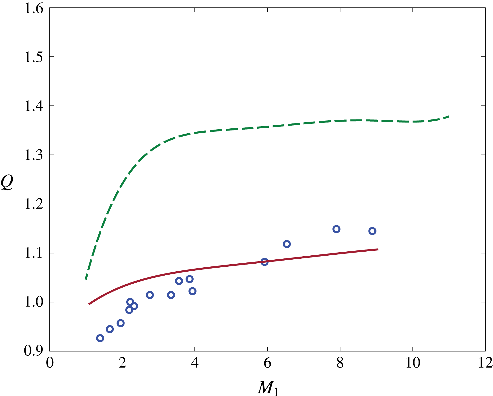
In figure 3 we provide the corresponding asymmetry of the density profiles for the argon gas, over the same Mach number range. Again, our result is in reasonable agreement with the experimental data, in particular when compared to the asymmetry resulting from the NSF theory.

Figure 3.

Asymmetry of density profiles, $Q$ , as a function of upstream Mach number, $M_{1}$ , in argon gas: ○, experimental results of Schmidt (Reference Schmidt1969) and Alsmeyer (Reference Alsmeyer1976); – – –, NSF theory; ——, present theory.

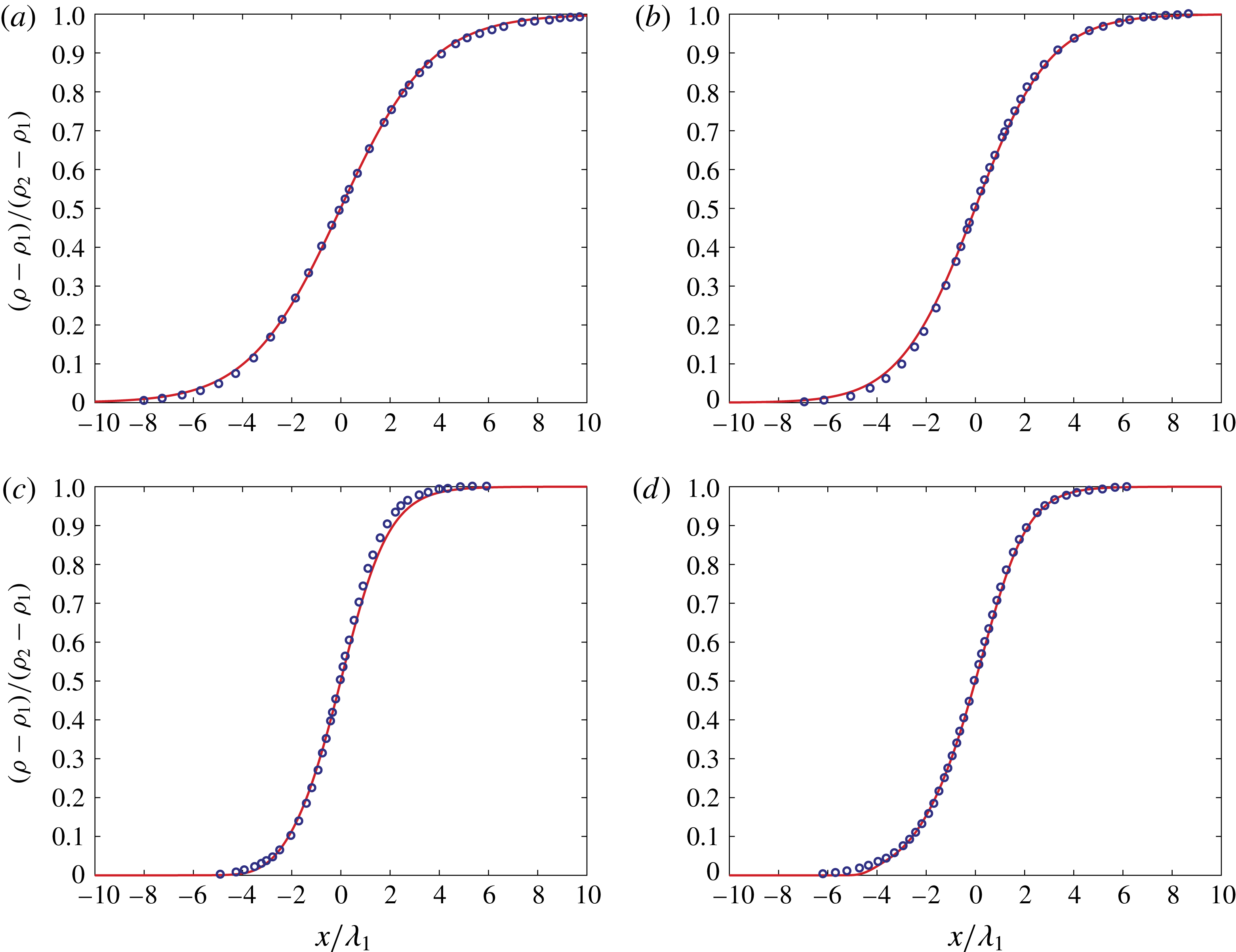
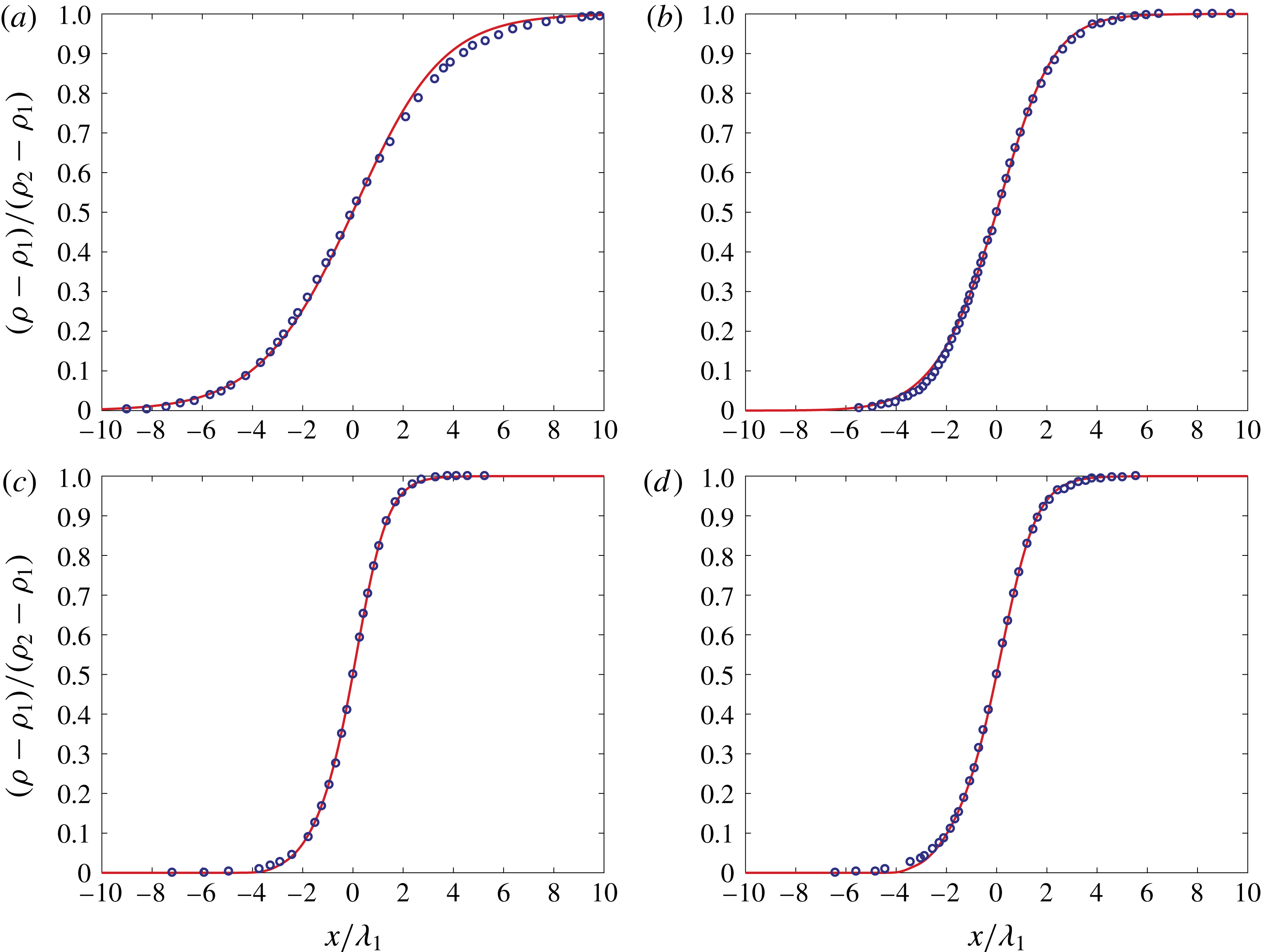
More critical comparisons for the argon gas are provided by comparing the actual density distributions. Such distributions for Mach numbers 1.55, 1.75, 3.8 and 9.0 are shown in figure 4. Our results are in excellent agreement with the experimental data of Alsmeyer (Reference Alsmeyer1976). With the exception of the DSMC results (see Alsmeyer Reference Alsmeyer1976), this is not the case for the distributions obtained from the various second-order expansions of the Boltzmann equation (e.g. Reese et al. Reference Reese, Woods, Thivet and Candel1995) or from the modified Brenner equation (see Greenshields & Reese Reference Greenshields and Reese2007).

Figure 4.

Shock density profiles in argon gas for (a) $M_{1}=1.55$ , (b) $M_{1}=1.75$ , (c) $M_{1}=3.8$ and (d) $M_{1}=9.0$ : ——, present theory; ○, experimental results of Alsmeyer (Reference Alsmeyer1976).

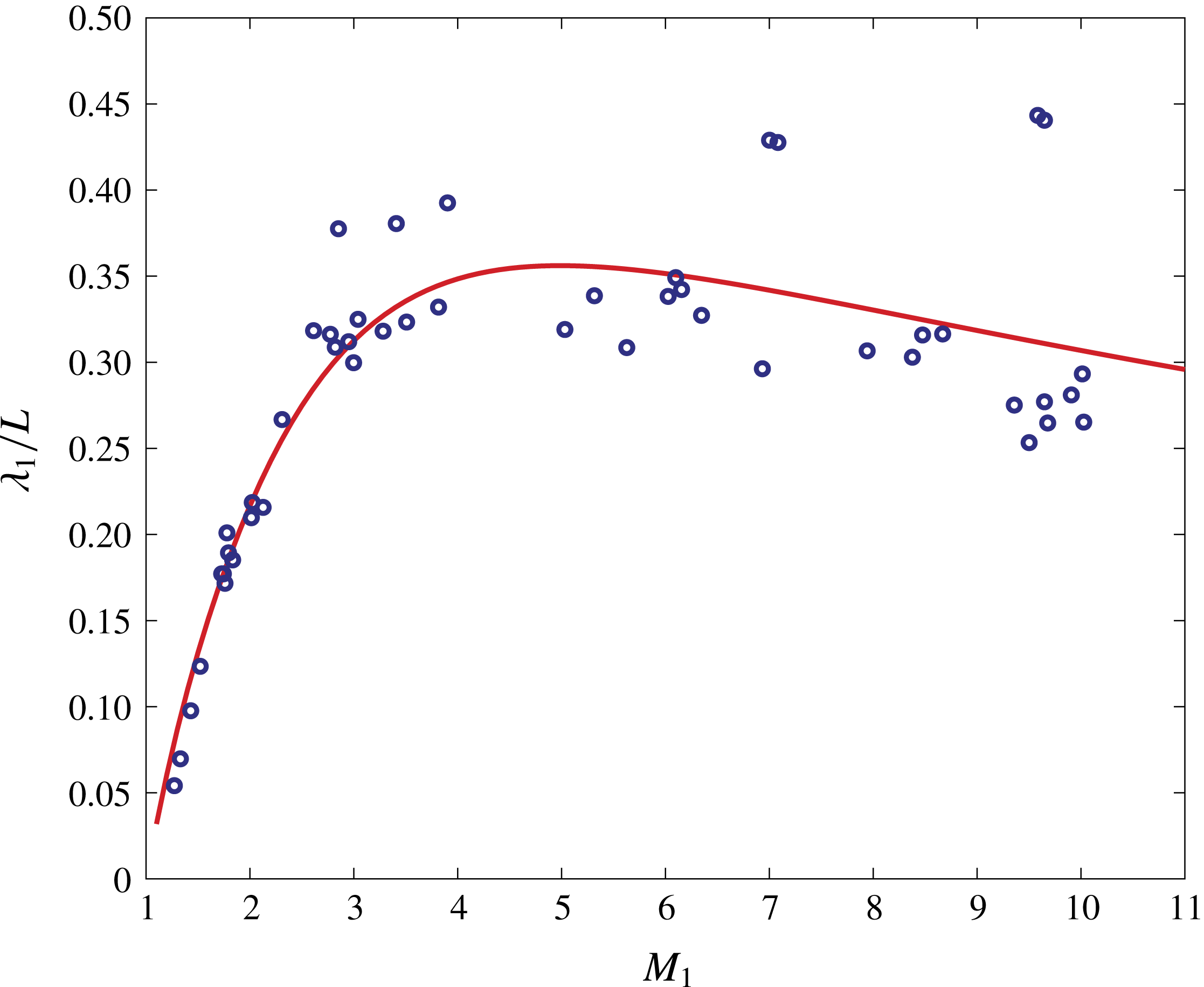
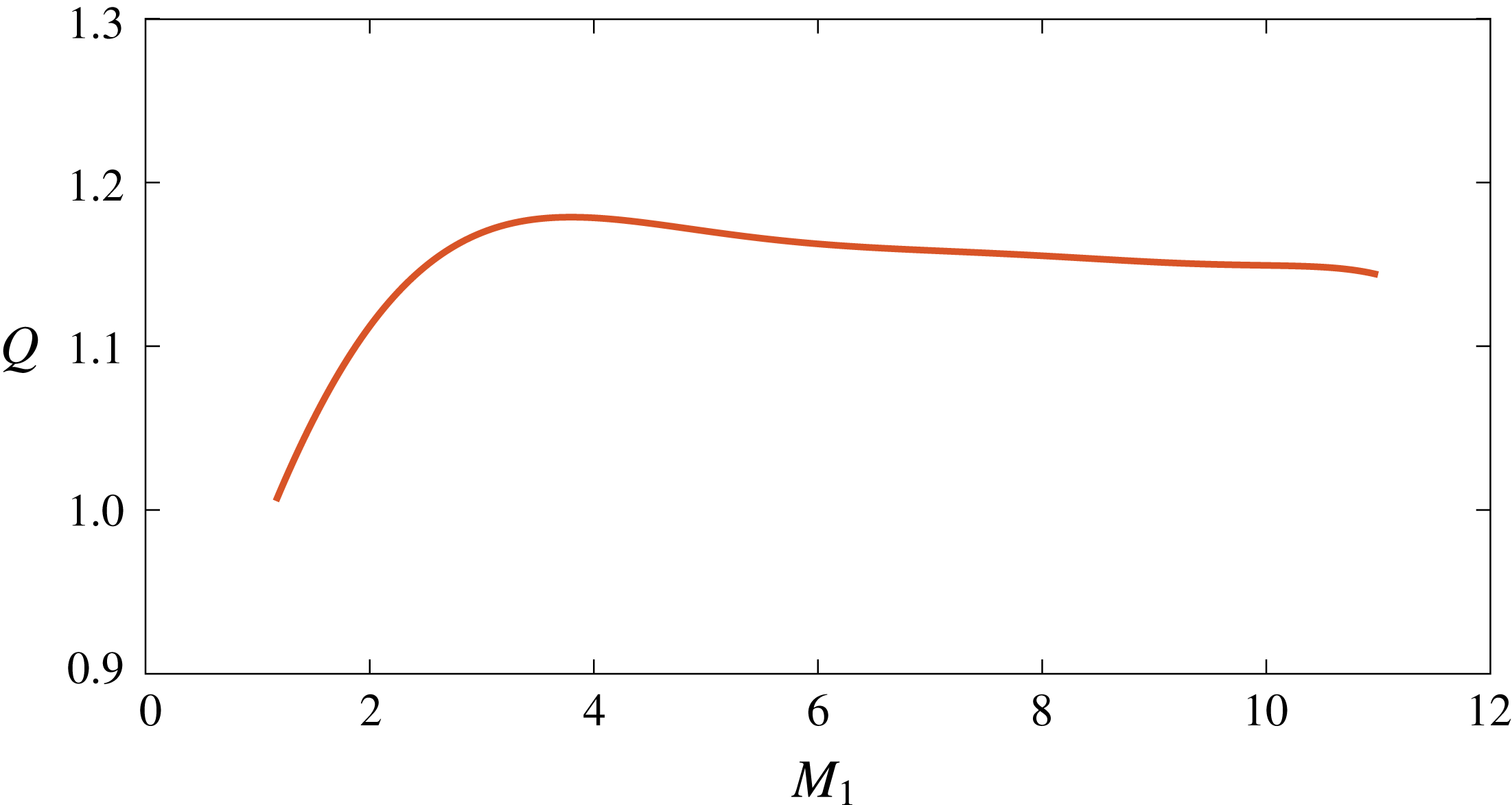
Analogous results, and comparisons to experimental data where available, for the inverse shock thickness, asymmetry of density profiles and density distributions for the same Mach numbers for nitrogen gas (in this case the bulk viscosity is not zero) are provided in figures 5, 6 and 7, respectively. We make the following observations. First, as in the case for argon, the inverse shock thickness for nitrogen is in relatively good agreement with the experimental results. Second, to the authors’ knowledge, no experimental results are available for the asymmetry of the density profiles for nitrogen, and thus we just provide the result obtained from the present second-order theory. Lastly, as observed from figure 7, for nitrogen gas we again have excellent agreement of the density profiles between our theory and experimental results.

Figure 5.

Inverse shock thickness, $\unicode[STIX]{x1D706}_{1}/L$ , as a function of upstream Mach number, $M_{1}$ , in nitrogen gas: ○, experimental results of Greene & Hornig (Reference Greene and Hornig1953), Linzer & Hornig (Reference Linzer and Hornig1963), Camac (Reference Camac and de Leeuw1965), Robben & Talbot (Reference Robben and Talbot1966) and Alsmeyer (Reference Alsmeyer1976); ——, present theory.

Figure 6.

Asymmetry of density profiles, $Q$ , as a function of upstream Mach number, $M_{1}$ , in nitrogen gas: ——, present theory.

Figure 7.

Shock density profiles in nitrogen gas for (a) $M_{1}=1.53$ , (b) $M_{1}=2.0$ , (c) $M_{1}=6.1$ and (d) $M_{1}=10.0$ : ——, present theory; ○, experimental results of Alsmeyer (Reference Alsmeyer1976).

6 Discussion and conclusions

We next compare our second-order continuum theory obtained through an expansion in strain rate and gradients of density and temperature with the second-order theory obtained through the Chapman–Enskog expansion in Knudsen number. To facilitate this, we rewrite our constitutive equations (4.6) and (4.7) in dimensional form but with dimensionless new parameters (which are functions of dimensionless density and temperature),

(6.1)

$$\begin{eqnarray}\displaystyle & \displaystyle q=-k\,\frac{\text{d}\unicode[STIX]{x1D703}}{\text{d}x}-{k^{\star }}^{\prime }\,\frac{\unicode[STIX]{x1D707}^{2}}{\unicode[STIX]{x1D70C}\,\unicode[STIX]{x1D703}}\,\frac{\text{d}u}{\text{d}x}\frac{\text{d}\unicode[STIX]{x1D703}}{\text{d}x}-{k^{\star \star }}^{\prime }\left(\frac{\unicode[STIX]{x1D707}}{\unicode[STIX]{x1D70C}}\right)^{2}\frac{\text{d}\unicode[STIX]{x1D70C}}{\text{d}x}\,\frac{\text{d}u}{\text{d}x}, & \displaystyle\end{eqnarray}$$

(6.2)

$$\begin{eqnarray}\displaystyle & \displaystyle \unicode[STIX]{x1D70E}=-p+\unicode[STIX]{x1D701}\,\frac{\text{d}u}{\text{d}x}-{k^{\star }}^{\prime }\frac{\unicode[STIX]{x1D707}^{2}}{\unicode[STIX]{x1D70C}\,\unicode[STIX]{x1D703}^{2}}\left(\frac{\text{d}\unicode[STIX]{x1D703}}{\text{d}x}\right)^{2}-{k^{\star \star }}^{\prime }\frac{\unicode[STIX]{x1D707}^{2}}{\unicode[STIX]{x1D70C}^{2}\unicode[STIX]{x1D703}}\,\frac{\text{d}\unicode[STIX]{x1D70C}}{\text{d}x}\,\frac{\text{d}\unicode[STIX]{x1D703}}{\text{d}x}, & \displaystyle\end{eqnarray}$$

so as to write them in the same form obtained through the Chapman–Enskog expansion for a monatomic gas (see Lumpkin & Chapman Reference Lumpkin and Chapman1992; Reese et al. Reference Reese, Woods, Thivet and Candel1995),

(6.3)

$$\begin{eqnarray}\displaystyle q & = & \displaystyle -k\,\frac{\text{d}\unicode[STIX]{x1D703}}{\text{d}x}+c_{1}\frac{\unicode[STIX]{x1D707}^{2}}{\unicode[STIX]{x1D70C}\,\unicode[STIX]{x1D703}}\frac{\text{d}u}{\text{d}x}\frac{\text{d}\unicode[STIX]{x1D703}}{\text{d}x}+c_{2}\left(\frac{\unicode[STIX]{x1D707}}{\unicode[STIX]{x1D70C}}\right)^{2}\frac{\text{d}\unicode[STIX]{x1D70C}}{\text{d}x}\,\frac{\text{d}u}{\text{d}x}-\underbrace{c_{3}\frac{\unicode[STIX]{x1D707}^{2}}{\unicode[STIX]{x1D70C}}\,\frac{\text{d}^{2}u}{\text{d}x^{2}}}_{(3)},\end{eqnarray}$$

(6.4)

$$\begin{eqnarray}\displaystyle \unicode[STIX]{x1D70E} & = & \displaystyle -p+\frac{4}{3}\,\unicode[STIX]{x1D707}\,\frac{\text{d}u}{\text{d}x}-\underbrace{c_{4}\frac{\unicode[STIX]{x1D707}^{2}}{p}\left(\frac{\text{d}u}{\text{d}x}\right)^{2}}_{(1)}-\,c_{5}\frac{\unicode[STIX]{x1D707}^{2}}{\unicode[STIX]{x1D70C}\,\unicode[STIX]{x1D703}^{2}}\left(\frac{\text{d}\unicode[STIX]{x1D703}}{\text{d}x}\right)^{2}+c_{6}\frac{\unicode[STIX]{x1D707}^{2}}{\unicode[STIX]{x1D70C}^{2}\unicode[STIX]{x1D703}}\frac{\text{d}\unicode[STIX]{x1D70C}}{\text{d}x}\,\frac{\text{d}\unicode[STIX]{x1D703}}{\text{d}x}\nonumber\\ \displaystyle & & \displaystyle -\,\underbrace{c_{7}\frac{\unicode[STIX]{x1D707}^{2}}{\unicode[STIX]{x1D70C}^{3}}\,\left(\frac{\text{d}\unicode[STIX]{x1D70C}}{\text{d}x}\right)^{2}}_{(2)}+\underbrace{c_{8}\frac{\unicode[STIX]{x1D707}^{2}}{\unicode[STIX]{x1D70C}\,\unicode[STIX]{x1D703}}\,\frac{\text{d}^{2}\unicode[STIX]{x1D703}}{\text{d}x^{2}}+c_{9}\frac{\unicode[STIX]{x1D707}^{2}}{\unicode[STIX]{x1D70C}^{2}}\,\frac{\text{d}^{2}\unicode[STIX]{x1D70C}}{\text{d}x^{2}}}_{(3)},\end{eqnarray}$$

where all $c_{i}$ values are dimensionless constants obtained from collision integrals. We have identified several terms in the latter equations to facilitate the following discussion. In comparing the constitutive equations, we first note that for a monatomic gas $\unicode[STIX]{x1D705}=0$ so that $\unicode[STIX]{x1D701}=4/3\,\unicode[STIX]{x1D707}$ . Subsequently, all terms in our constitutive equations (6.1) and (6.2) are also present in the corresponding equations (6.3) and (6.4). But, the constitutive equations obtained from kinetic theory have additional terms that we discuss below.

Term (1), which is quadratic in the velocity gradient, does not appear in (6.2) since the two terms that are quadratic in the velocity gradient in (4.5) cancel in the one-dimensional problem of the shock structure. This would suggest that $c_{4}$ in (6.4) should be zero; Lumpkin & Chapman (Reference Lumpkin and Chapman1992) (see also Reese et al. Reference Reese, Woods, Thivet and Candel1995) report $c_{4}=-12.31$ .

Term (2), which is quadratic in the density gradient, does not appear in (6.2). While such terms do appear in the general second-order representation (3.24) (see the terms multiplied by $a_{0002}$ and $a_{60}$ ), the reduced entropy inequality (3.26) requires that $a_{0002}=a_{60}=0$ . This would suggest that $c_{7}$ should be zero; Lumpkin and Chapman report $c_{7}=1.75$ . Our conclusion regarding this term is consistent with the results of Comeaux et al. (Reference Comeaux, Chapman and MacCormack1995) who showed that the Burnett equations can violate the second law of thermodynamics and this may be the cause for the instability encountered in their solution.

All terms (3) involving second derivatives result from the Knudsen number expansion and do not appear in our continuum second-order representation. We note that their presence has been recognized by Reese et al. (Reference Reese, Woods, Thivet and Candel1995) as the source of oscillations in the shock structure profiles, which are not evident in experimental results.

In this work we have used standard continuum balance equations for mass, linear momentum and energy. In conjunction with the entropy inequality, we have extended the constitutive equations necessitated by these equations to second order, but not in Knudsen numbers, but in strain rate and gradients of density and temperature. The solutions for the shock wave structure indicate that at higher Mach numbers our extended constitutive equations are more accurate than classical linear ones for argon and nitrogen gases. Furthermore, they are also more robust and accurate than equations obtained from expansions of the Boltzmann equation in Knudsen number or equations arising from diffusion of volume arguments.

One advantage of the present second-order constitutive relations is that, in principle, solving them should not be much more computationally expensive than solving the standard NSF equations, so complex simulations in three dimensions should be tractable. Another advantage is that these new constitutive equations reduce to the linear constitutive equations in area of low flow gradients. Therefore, the same set of equations can be applied across an entire flow field in hypersonic flow. Additional accuracy could be obtained from use of a non-ideal gas equation of state. Lastly, for application to general flows, the individual properties $\unicode[STIX]{x1D707}^{\prime }$ , $k^{\prime }$ , $k^{\prime \prime }$ , $k^{\prime \prime \prime }$ and $k^{\prime \prime \prime \prime }$ (as functions of $\unicode[STIX]{x1D70C}$ and $\unicode[STIX]{x1D703}$ ) are required. Their experimental measurements would necessitate simple solutions of the present extended theory in cases where such properties can be clearly identified.

Appendix A

Recognizing that the constitutive quantities (3.3) depend on the basic fields (3.4), using the chain rule, we can write

(A 1)

$$\begin{eqnarray}\displaystyle & \displaystyle \dot{\unicode[STIX]{x1D713}}=\frac{\unicode[STIX]{x2202}\unicode[STIX]{x1D713}}{\unicode[STIX]{x2202}\unicode[STIX]{x1D70C}}\,\dot{\unicode[STIX]{x1D70C}}+\frac{\unicode[STIX]{x2202}\unicode[STIX]{x1D713}}{\unicode[STIX]{x2202}r_{i}}\,{\dot{r}}_{i}+\frac{\unicode[STIX]{x2202}\unicode[STIX]{x1D713}}{\unicode[STIX]{x2202}\unicode[STIX]{x1D60B}_{ij}}\,\unicode[STIX]{x1D60B}_{ij}+\frac{\unicode[STIX]{x2202}\unicode[STIX]{x1D713}}{\unicode[STIX]{x2202}\unicode[STIX]{x1D703}}\,\dot{\unicode[STIX]{x1D703}}+\frac{\unicode[STIX]{x2202}\unicode[STIX]{x1D713}}{\unicode[STIX]{x2202}g_{i}}\,{\dot{g}}_{i}, & \displaystyle\end{eqnarray}$$

(A 2)

$$\begin{eqnarray}\displaystyle & \displaystyle k_{i,i}=\frac{\unicode[STIX]{x2202}k_{i}}{\unicode[STIX]{x2202}\unicode[STIX]{x1D70C}}\,\unicode[STIX]{x1D70C}_{,i}+\frac{\unicode[STIX]{x2202}k_{i}}{\unicode[STIX]{x2202}r_{j}}\,r_{j,i}+\frac{\unicode[STIX]{x2202}k_{i}}{\unicode[STIX]{x2202}\unicode[STIX]{x1D60B}_{jk}}\,\unicode[STIX]{x1D60B}_{jk,i}+\frac{\unicode[STIX]{x2202}k_{i}}{\unicode[STIX]{x2202}\unicode[STIX]{x1D703}}\,\unicode[STIX]{x1D703}_{,i}+\frac{\unicode[STIX]{x2202}k_{i}}{\unicode[STIX]{x2202}g_{j}}\,g_{j,i}. & \displaystyle\end{eqnarray}$$

Substituting (A 1) and (A 2) into the Clausius–Duhem inequality (3.1), and considering that from the local mass balance (2.1) we have $\dot{\unicode[STIX]{x1D70C}}=-\unicode[STIX]{x1D70C}\,v_{j,j}=-\unicode[STIX]{x1D70C}\,\unicode[STIX]{x1D60B}_{jj}$ and ${\dot{r}}_{i}=-(r_{j}\,L_{ji}+\unicode[STIX]{x1D70C}\,\unicode[STIX]{x1D60B}_{jj,i}+r_{i}\,\unicode[STIX]{x1D60B}_{jj})$ , where $L_{ij}=\unicode[STIX]{x1D60B}_{ij}+\unicode[STIX]{x1D61E}_{ij}$ ,

(A 3a,b )

$$\begin{eqnarray}\displaystyle \unicode[STIX]{x1D60B}_{ij}={\textstyle \frac{1}{2}}(v_{i,j}+v_{j,i})\quad \text{and}\quad \unicode[STIX]{x1D61E}_{ij}={\textstyle \frac{1}{2}}(v_{i,j}-v_{j,i}), & & \displaystyle\end{eqnarray}$$

we arrive at

(A 4)

$$\begin{eqnarray}\displaystyle \unicode[STIX]{x1D6FE}_{v}\unicode[STIX]{x1D703} & = & \displaystyle -\unicode[STIX]{x1D70C}\left(\unicode[STIX]{x1D702}+\frac{\unicode[STIX]{x2202}\unicode[STIX]{x1D713}}{\unicode[STIX]{x2202}\unicode[STIX]{x1D703}}\right)\dot{\unicode[STIX]{x1D703}}+\left[\unicode[STIX]{x1D70C}\left(\unicode[STIX]{x1D70C}\,\frac{\unicode[STIX]{x2202}\unicode[STIX]{x1D713}}{\unicode[STIX]{x2202}\unicode[STIX]{x1D70C}}+r_{k}\,\frac{\unicode[STIX]{x2202}\unicode[STIX]{x1D713}}{\unicode[STIX]{x2202}\unicode[STIX]{x1D70C}_{k}}\right)\unicode[STIX]{x1D6FF}_{ij}+\unicode[STIX]{x1D70C}\,\frac{\unicode[STIX]{x2202}\unicode[STIX]{x1D713}}{\unicode[STIX]{x2202}\unicode[STIX]{x1D70C}_{i}}\,r_{j}+\unicode[STIX]{x1D70E}_{ij}\right]\unicode[STIX]{x1D60B}_{ij}\nonumber\\ \displaystyle & & \displaystyle -\left(\unicode[STIX]{x1D70C}\,\frac{\unicode[STIX]{x2202}\unicode[STIX]{x1D713}}{\unicode[STIX]{x2202}r_{i}}\,r_{j}\right)\unicode[STIX]{x1D61E}_{ij}+\left(\unicode[STIX]{x1D70C}^{2}\,\frac{\unicode[STIX]{x2202}\unicode[STIX]{x1D713}}{\unicode[STIX]{x2202}r_{i}}\,\unicode[STIX]{x1D6FF}_{jk}+\unicode[STIX]{x1D703}\,\frac{\unicode[STIX]{x2202}k_{i}}{\unicode[STIX]{x2202}\unicode[STIX]{x1D60B}_{jk}}\right)\unicode[STIX]{x1D60B}_{jk,i}-\left(\unicode[STIX]{x1D70C}\,\frac{\unicode[STIX]{x2202}\unicode[STIX]{x1D713}}{\unicode[STIX]{x2202}\unicode[STIX]{x1D60B}_{ij}}\right)\unicode[STIX]{x1D60B}_{ij}-\left(\unicode[STIX]{x1D70C}\,\frac{\unicode[STIX]{x2202}\unicode[STIX]{x1D713}}{\unicode[STIX]{x2202}g_{i}}\right)\dot{g_{i}}\nonumber\\ \displaystyle & & \displaystyle +\left(\unicode[STIX]{x1D703}\,\frac{\unicode[STIX]{x2202}k_{i}}{\unicode[STIX]{x2202}\unicode[STIX]{x1D70C}}\right)r_{i}+\left(\unicode[STIX]{x1D703}\,\frac{\unicode[STIX]{x2202}k_{i}}{\unicode[STIX]{x2202}r_{j}}\right)r_{j,i}+\left(\unicode[STIX]{x1D703}\,\frac{\unicode[STIX]{x2202}k_{i}}{\unicode[STIX]{x2202}g_{j}}\right)g_{j,i}-\left(\frac{q_{i}}{\unicode[STIX]{x1D703}}-\unicode[STIX]{x1D703}\,\frac{\unicode[STIX]{x2202}k_{i}}{\unicode[STIX]{x2202}\unicode[STIX]{x1D703}}\right)g_{i}\geqslant 0.\end{eqnarray}$$

Now the constitutive quantities $\{\unicode[STIX]{x1D713},\unicode[STIX]{x1D702},q_{i},k_{j},\unicode[STIX]{x1D70E}_{kl}\}$ are fixed if we fix the independent variables $\{\unicode[STIX]{x1D70C},\boldsymbol{r}_{i},\unicode[STIX]{x1D60B}_{jk},\unicode[STIX]{x1D703},g_{l}\}$ . Subsequently, we note that from frame invariance the constitutive quantities cannot depend on $\unicode[STIX]{x1D61E}_{ij}$ , and furthermore the above equation will then depend linearly on $\dot{\unicode[STIX]{x1D703}}$ , $\unicode[STIX]{x1D60B}_{ik}$ , $\dot{g_{i}}$ , $r_{j,i}$ , $\unicode[STIX]{x1D60B}_{ik,i}$ and $g_{j,i}$ which can still be made to vary arbitrarily and to have any sign. Thus, satisfaction of (A 4) is assured only if

(A 5)

$$\begin{eqnarray}\displaystyle & \displaystyle \unicode[STIX]{x1D70C}\left(\unicode[STIX]{x1D702}+\frac{\unicode[STIX]{x2202}\unicode[STIX]{x1D713}}{\unicode[STIX]{x2202}\unicode[STIX]{x1D703}}\right)=0, & \displaystyle\end{eqnarray}$$

(A 6)

$$\begin{eqnarray}\displaystyle & \displaystyle \unicode[STIX]{x1D70C}\left(\frac{\unicode[STIX]{x2202}\unicode[STIX]{x1D713}}{\unicode[STIX]{x2202}r_{i}}\,r_{j}-\frac{\unicode[STIX]{x2202}\unicode[STIX]{x1D713}}{\unicode[STIX]{x2202}r_{j}}\,r_{i}\right)=0, & \displaystyle\end{eqnarray}$$

(A 7)

$$\begin{eqnarray}\displaystyle & \displaystyle \unicode[STIX]{x1D70C}^{2}\,\frac{\unicode[STIX]{x2202}\unicode[STIX]{x1D713}}{\unicode[STIX]{x2202}r_{i}}\,\unicode[STIX]{x1D6FF}_{jk}+\unicode[STIX]{x1D703}\,\frac{\unicode[STIX]{x2202}k_{i}}{\unicode[STIX]{x2202}\unicode[STIX]{x1D60B}_{jk}}=0, & \displaystyle\end{eqnarray}$$

(A 8)

$$\begin{eqnarray}\displaystyle & \displaystyle \unicode[STIX]{x1D70C}\,\frac{\unicode[STIX]{x2202}\unicode[STIX]{x1D713}}{\unicode[STIX]{x2202}\unicode[STIX]{x1D60B}_{ij}}=0, & \displaystyle\end{eqnarray}$$

(A 9)

$$\begin{eqnarray}\displaystyle & \displaystyle \unicode[STIX]{x1D70C}\,\frac{\unicode[STIX]{x2202}\unicode[STIX]{x1D713}}{\unicode[STIX]{x2202}g_{i}}=0, & \displaystyle\end{eqnarray}$$

(A 10)

$$\begin{eqnarray}\displaystyle & \displaystyle \unicode[STIX]{x1D703}\left(\frac{\unicode[STIX]{x2202}k_{i}}{\unicode[STIX]{x2202}r_{j}}+\frac{\unicode[STIX]{x2202}k_{j}}{\unicode[STIX]{x2202}r_{i}}\right)=0, & \displaystyle\end{eqnarray}$$

(A 11)

$$\begin{eqnarray}\displaystyle & \displaystyle \unicode[STIX]{x1D703}\left(\frac{\unicode[STIX]{x2202}k_{i}}{\unicode[STIX]{x2202}g_{j}}+\frac{\unicode[STIX]{x2202}k_{j}}{\unicode[STIX]{x2202}g_{i}}\right)=0, & \displaystyle\end{eqnarray}$$

with (A 4) reducing to

(A 12)

$$\begin{eqnarray}\displaystyle \unicode[STIX]{x1D6FE}_{v}\unicode[STIX]{x1D703} & = & \displaystyle \left[\unicode[STIX]{x1D70C}\left(\unicode[STIX]{x1D70C}\,\frac{\unicode[STIX]{x2202}\unicode[STIX]{x1D713}}{\unicode[STIX]{x2202}\unicode[STIX]{x1D70C}}+r_{k}\,\frac{\unicode[STIX]{x2202}\unicode[STIX]{x1D713}}{\unicode[STIX]{x2202}r_{k}}\right)\unicode[STIX]{x1D6FF}_{ij}+\unicode[STIX]{x1D70C}\,\frac{\unicode[STIX]{x2202}\unicode[STIX]{x1D713}}{\unicode[STIX]{x2202}r_{i}}\,r_{j}+\unicode[STIX]{x1D70E}_{ij}\right]\unicode[STIX]{x1D60B}_{ij}\nonumber\\ \displaystyle & & \displaystyle +\left(\unicode[STIX]{x1D703}\,\frac{\unicode[STIX]{x2202}k_{i}}{\unicode[STIX]{x2202}\unicode[STIX]{x1D70C}}\right)r_{i}-\left(\frac{q_{i}}{\unicode[STIX]{x1D703}}-\unicode[STIX]{x1D703}\,\frac{\unicode[STIX]{x2202}k_{i}}{\unicode[STIX]{x2202}\unicode[STIX]{x1D703}}\right)g_{i}\geqslant 0.\end{eqnarray}$$

In writing (A 6), (A 10) and (A 11) we have used the fact that the components of tensors $\unicode[STIX]{x1D61E}_{ij}$ are skew-symmetric, while those of $r_{j,i}$ and $g_{j,i}$ are symmetric.

Now, since $\unicode[STIX]{x1D70C}>0$ , from (A 8) and (A 9) we have that

(A 13)

$$\begin{eqnarray}\displaystyle \unicode[STIX]{x1D713}=\unicode[STIX]{x1D713}(\unicode[STIX]{x1D70C},r_{i},\unicode[STIX]{x1D703}) & & \displaystyle\end{eqnarray}$$

or, since $\unicode[STIX]{x1D713}$ must be an isotropic function of the invariant of $r_{i}$ , i.e. $I_{7}\equiv r_{i}\,r_{i}$ , we have

(A 14)

$$\begin{eqnarray}\displaystyle \unicode[STIX]{x1D713}=\unicode[STIX]{x1D713}(\unicode[STIX]{x1D70C},\unicode[STIX]{x1D703},I_{7}). & & \displaystyle\end{eqnarray}$$

In addition, from (A 5) we have that

(A 15)

$$\begin{eqnarray}\displaystyle \unicode[STIX]{x1D702}=-\frac{\unicode[STIX]{x2202}\unicode[STIX]{x1D713}}{\unicode[STIX]{x2202}\unicode[STIX]{x1D703}}, & & \displaystyle\end{eqnarray}$$

and, since $\unicode[STIX]{x1D703}>0$ , from (A 7) that

(A 16)

$$\begin{eqnarray}\displaystyle k_{i}=\widehat{k}_{i}-\frac{\unicode[STIX]{x1D70C}^{2}}{\unicode[STIX]{x1D703}}\,\frac{\unicode[STIX]{x2202}\unicode[STIX]{x1D713}}{\unicode[STIX]{x2202}r_{i}}\,\unicode[STIX]{x1D60B}_{kk}, & & \displaystyle\end{eqnarray}$$

where $\widehat{k}_{i}$ is independent of $\unicode[STIX]{x1D60B}_{jk}$ . Substituting (A 14) and (A 16) into (A 10) we obtain

(A 17)

$$\begin{eqnarray}\displaystyle \unicode[STIX]{x1D703}\left(\frac{\unicode[STIX]{x2202}\widehat{k}_{i}}{\unicode[STIX]{x2202}r_{j}}+\frac{\unicode[STIX]{x2202}\widehat{k}_{j}}{\unicode[STIX]{x2202}r_{i}}\right)-2\,\unicode[STIX]{x1D70C}^{2}\,\frac{\unicode[STIX]{x2202}^{2}\unicode[STIX]{x1D713}}{\unicode[STIX]{x2202}r_{i}\unicode[STIX]{x2202}r_{j}}\,\unicode[STIX]{x1D60B}_{kk}=0. & & \displaystyle\end{eqnarray}$$

Now since $\unicode[STIX]{x1D713}$ and $\widehat{k}_{i}$ are independent of $\unicode[STIX]{x1D60B}_{jk}$ , we must have that

(A 18a,b )

$$\begin{eqnarray}\displaystyle \frac{\unicode[STIX]{x2202}^{2}\unicode[STIX]{x1D713}}{\unicode[STIX]{x2202}r_{i}\unicode[STIX]{x2202}r_{j}}=0\quad \text{and}\quad \frac{\unicode[STIX]{x2202}\widehat{k}_{i}}{\unicode[STIX]{x2202}r_{j}}+\frac{\unicode[STIX]{x2202}\widehat{k}_{j}}{\unicode[STIX]{x2202}r_{i}}=0. & & \displaystyle\end{eqnarray}$$

It subsequently follows from (A 14), (A 16) and (A 18) that

(A 19a,b )

$$\begin{eqnarray}\displaystyle \unicode[STIX]{x1D713}=\unicode[STIX]{x1D713}\left(\unicode[STIX]{x1D70C},\unicode[STIX]{x1D703}\right)\quad \text{and thus}\quad k_{i}=\widehat{k}_{i}. & & \displaystyle\end{eqnarray}$$

It now remains to exploit (A 10) and (A 11) and recall that $k_{i}$ is independent of $\unicode[STIX]{x1D60B}_{jk}$ . We first note that both equations are of the form

(A 20)

$$\begin{eqnarray}\displaystyle \frac{\unicode[STIX]{x2202}f_{i}}{\unicode[STIX]{x2202}y_{j}}+\frac{\unicode[STIX]{x2202}f_{j}}{\unicode[STIX]{x2202}y_{i}}=0 & & \displaystyle\end{eqnarray}$$

whose general solution is given by

(A 21)

$$\begin{eqnarray}\displaystyle f_{i}=a_{i}+A_{ij}\,y_{j}, & & \displaystyle\end{eqnarray}$$

where $A_{ij}$ is skew-symmetric, and both $a_{i}$ and $A_{ij}$ are independent of $y_{k}$ .

Now, from (A 10) we have that

(A 22)

$$\begin{eqnarray}\displaystyle k_{i}=a_{i}+A_{ij}\,r_{j}, & & \displaystyle\end{eqnarray}$$

where $A_{ij}$ is skew-symmetric and both $a_{i}$ and $A_{ij}$ are independent of $r_{k}$ . Substituting (A 22) into (A 11) we obtain

(A 23)

$$\begin{eqnarray}\displaystyle \left(\frac{\unicode[STIX]{x2202}a_{i}}{\unicode[STIX]{x2202}g_{k}}+\frac{\unicode[STIX]{x2202}a_{k}}{\unicode[STIX]{x2202}g_{i}}\right)+\left(\frac{\unicode[STIX]{x2202}A_{ij}}{\unicode[STIX]{x2202}g_{k}}+\frac{\unicode[STIX]{x2202}A_{kj}}{\unicode[STIX]{x2202}g_{i}}\right)r_{j}=0. & & \displaystyle\end{eqnarray}$$

It follows that

(A 24a,b )

$$\begin{eqnarray}\displaystyle \frac{\unicode[STIX]{x2202}a_{i}}{\unicode[STIX]{x2202}g_{k}}+\frac{\unicode[STIX]{x2202}a_{k}}{\unicode[STIX]{x2202}g_{i}}=0\quad \text{and}\quad \frac{\unicode[STIX]{x2202}A_{ij}}{\unicode[STIX]{x2202}g_{k}}+\frac{\unicode[STIX]{x2202}A_{kj}}{\unicode[STIX]{x2202}g_{i}}=0. & & \displaystyle\end{eqnarray}$$

Subsequently,

(A 25a,b )

$$\begin{eqnarray}\displaystyle a_{i}=b_{i}+B_{ij}\,g_{j}\quad \text{and}\quad A_{ij}=c_{ij}+C_{ijk}\,g_{k}, & & \displaystyle\end{eqnarray}$$

where $B_{ij}$ and $c_{ij}$ are skew-symmetric, $C_{ijk}$ is completely skew-symmetric and $b_{i}$ , $B_{ij}$ , $c_{ij}$ and $C_{ijk}$ are independent of $g_{l}$ , or more appropriately, they are only functions of $\unicode[STIX]{x1D70C}$ and $\unicode[STIX]{x1D703}$ . Substituting (A 25) into (A 22) we have

(A 26)

$$\begin{eqnarray}\displaystyle k_{i}=b_{i}+c_{ij}\,r_{j}+B_{ij}\,g_{j}+C_{ijk}\,r_{j}\,g_{k}. & & \displaystyle\end{eqnarray}$$

However, there are no objective isotropic tensors of ranks 1, 2 and 3 that are only functions of the scalars $\unicode[STIX]{x1D70C}$ and $\unicode[STIX]{x1D703}$ . Subsequently, $b_{i}=c_{ij}=B_{ij}=C_{ijk}=0$ and thus $k_{i}=0$ , or from (3.2)

(A 27)

$$\begin{eqnarray}\displaystyle h_{i}=\frac{q_{i}}{\unicode[STIX]{x1D703}}. & & \displaystyle\end{eqnarray}$$

Lastly, we note that the reduced entropy inequality (A 12) reduces to

(A 28)

$$\begin{eqnarray}\displaystyle \unicode[STIX]{x1D6FE}\,\unicode[STIX]{x1D703}=\left(\unicode[STIX]{x1D70C}^{2}\,\frac{\unicode[STIX]{x2202}\unicode[STIX]{x1D713}}{\unicode[STIX]{x2202}\unicode[STIX]{x1D70C}}\,\unicode[STIX]{x1D6FF}_{ij}+\unicode[STIX]{x1D70E}_{ij}\right)\unicode[STIX]{x1D60B}_{ij}-\frac{q_{i}}{\unicode[STIX]{x1D703}}\,g_{i}\geqslant 0. & & \displaystyle\end{eqnarray}$$

References

Alsmeyer, H. 1976 Density profiles in argon and nitrogen shock waves measured by the absorption of an electron beam. J. Fluid Mech. 74 (3), 497–513.Google Scholar

Balakrishnan, R. 2004 An approach to entropy consistency in second-order hydrodynamic equations. J. Fluid Mech. 503, 201–245.CrossRef Google Scholar

Balakrishnan, R. & Agarwal, R. K. 1999 A comparative study of several higher-order kinetic formulations beyond Navier–Stokes for computing the shock structure. In 37th AIAA Aerospace Sciences Meeting and Exhibit, AIAA-99-0224. American Institute of Aeronautics and Astronautics.Google Scholar

Bird, G. A. 1970 Aspects of the structure of strong shock waves. Phys. Fluids 13 (5), 1172–1177.CrossRef Google Scholar

Brau, C. A. 1967 Kinetic theory of polyatomic gases: models for the collision processes. Phys. Fluids 10, 48–55.Google Scholar

Brenner, H. 2005a Kinematics of volume transport. Physica A 349 (1–2), 11–59.CrossRef Google Scholar

Brenner, H. 2005b Navier–Stokes revisited. Physica A 349 (1–2), 60–132.Google Scholar

Camac, M. 1965 Argon and nitrogen shock thicknesses. In Proceedings of the Fourth International Symposium on Rarefied Gas Dynamics (ed. de Leeuw, J. H.), vol. 1, p. 240. Academic Press.Google Scholar

Chapman, S. & Cowling, T. G. 1970 The Mathematical Theory of Non-Uniform Gases. Cambridge University Press.Google Scholar

Chen, J. 2013 Extension of nonlinear Onsager theory of irreversibility. Acta Mechanica 224, 31533158.CrossRef Google Scholar

Coleman, B. D., Markovitz, H. & Noll, W. 1966 Viscometric Flows of Non-Newtonian Fluids. Springer.Google Scholar

Coleman, B. D. & Noll, W. 1961 Foundations of linear viscoelasticity. Rev. Mod. Phys. 33 (2), 239–249.Google Scholar

Comeaux, K. A., Chapman, D. R. & MacCormack, R. W. 1995 An analysis of the Burnett equations based on the second law of thermodynamics. In 33rd AIAA Aerospace Sciences Meeting and Exhibit, AIAA-95-0415. American Institute of Aeronautics and Astronautics.Google Scholar

Eringen, A. C. 1980 Mechanics of Continua. Krieger.Google Scholar

Eringen, A. C. 1999 Microcontinuum Field Theories I: Foundations and Solids. Springer.Google Scholar

Eringen, A. C. 2001 Microcontinuum Field Theories II: Fluent Media. Springer.Google Scholar

Garen, W., Synofzik, R. & Frohn, A. 1974 Shock-tube for generating weak shock-waves. AIAA J. 12 (8), 1132–1134.Google Scholar

Gilbarg, D. 1951 The existence and limit behavior of the one-dimensional shock layer. Am. J. Maths 73 (2), 256–274.Google Scholar

Gilbarg, D. & Paolucci, D. 1953 The structure of shock waves in the continuum theory of fluids. J. Ration. Mech. Anal. 2 (4), 617–642.Google Scholar

Grad, H. 1949 On the kinetic theory of rarefied gases. Commun. Pure Appl. Maths 2 (4), 331–407.Google Scholar

Grad, H. 1952 The profile of a steady plane shock wave. Commun. Pure Appl. Maths 5 (3), 257–300.Google Scholar

Greene, E. F. & Hornig, D. F. 1953 The shape and thickness of shock fronts in argon, hydrogen, nitrogen, and oxygen. J. Chem. Phys. 21 (4), 617–624.Google Scholar

Greenshields, C. J. & Reese, J. M. 2007 The structure of shock waves as a test of Brenner’s modifications to the Navier–Stokes equations. J. Fluid Mech. 580, 407–429.Google Scholar

Jin, S & Slemrod, M 2001 Regularization of the Burnett equations via relaxation. J. Stat. Phys. 103 (5–6), 1009–1033.Google Scholar

Khonkin, A. D. & Orlov, A. V. 1993 Weak shock structure on the basis of modified hydrodynamical equations. Phys. Fluids A 5 (7), 1810–1813.CrossRef Google Scholar

Landau, L. D. & Lifshitz, E. M. 1959 Fluid Mechanics, Course of Theoretical Physics, vol. 6. Pergamon Press.Google Scholar

Liepmann, H. W., Narasimha, R. & Chahine, M. T. 1962 Structure of a plane shock layer. Phys. Fluids 5 (11), 1313–1324.CrossRef Google Scholar

Linzer, M. & Hornig, D. F. 1963 Structure of shock fronts in argon and nitrogen. Phys. Fluids 6 (12), 1661–1668.Google Scholar

Liu, I.-S. 2002 Continuum Mechanics. Springer.Google Scholar

Liu, I.-S. & Salvador, J. A. 1990 Hyperbolic system for viscous fluids and simulation of shock tube flows. Contin. Mech. Thermodyn. 2 (3), 179–197.Google Scholar

Ludford, G. S. S. 1951 The classification of one-dimensional flows and the general shock problem of a compressible, viscous, heat-conducting fluid. J. Aero. Sci. 18 (12), 830–834.Google Scholar

Lumpkin, F. E. & Chapman, D. R. 1992 Accuracy of the Burnett equations for hypersonic real gas flows. J. Thermophys. Heat Transfer 6 (3), 419–425.Google Scholar

von Mises, R. 1950 On the thickness of a steady shock wave. J. Aero. Sci. 17 (9), 551–554; 594.Google Scholar

Morduchow, M. & Libby, P. A. 1949 On a complete solution of the one-dimensional flow equations of a viscous, heat-conducting, compressible gas. J. Aero. Sci. 16 (11), 674–684; 704.CrossRef Google Scholar

Paolucci, S. 2016 Continuum Mechanics and Thermodynamics of Matter. Cambridge University Press.CrossRef Google Scholar

Reese, J. M., Woods, L. C., Thivet, F. J. P. & Candel, S. M. 1995 A second-order description of shock structure. J. Comput. Phys. 117 (2), 240–250.Google Scholar

Rieutord, E.1970 Contribution à l’étude de l’onde de choc primaire en tube à choc. PhD thesis, Institut National des Sciences Appliquées de Lyon.Google Scholar

Robben, F. & Talbot, L. 1966 Measurement of shock wave thickness by electron beam fluorescence method. Phys. Fluids 9 (4), 633–643.Google Scholar

Russell, D.1965 In Proceedings of the Fourth International Symposium on Rarefied Gas Dynamics (ed. J. H. de Leeuw), vol. 1, p. 265. Academic Press.Google Scholar

Salomons, E. & Mareschal, M. 1992 Usefulness of the Burnett description of strong shock waves. Phys. Rev. Lett. 69 (2), 269–272.Google Scholar

Schmidt, B. 1969 Electron beam density measurements in shock waves in argon. J. Fluid Mech. 39 (2), 361–373.Google Scholar

Schultz-Grunow, F. & Frohn, A. 1965 In Proceedings of the Fourth International Symposium on Rarefied Gas Dynamics (ed. de Leeuw, J. H.), vol. 1, p. 250. Academic Press.Google Scholar

She, R. S. & Sather, N. F. 1967 Kinetic theory of polyatomic gases. J. Chem. Phys. 47, 4978–4993.Google Scholar

Sherman, F. S.1955 A low-density wind-tunnel study of shock-wave structure and relaxation phenomena in gases. NACA Technical Note 3298. National Advisory Committee for Aeronautics.Google Scholar

Struchtrup, H. & Torrilhon, M. 2003 Regularization of Grad’s 13 moment equations: derivation and linear analysis. Phys. Fluids 15 (9), 2668–2680.Google Scholar

Taniguchi, S., Arima, T., Ruggeri, T. & Sujiyama, M. 2014a Shock wave structure in a rarefied polyatomic gas based on extended thermodynamics. Acta Appl. Maths 132 (1), 583–593.CrossRef Google Scholar

Taniguchi, S., Arima, T., Ruggeri, T. & Sujiyama, M. 2014b Thermodynamic theory of the shock wave structure in a rarefied polyatomic gas: beyond the Bethe–Teller theory. Phys. Rev. E 89, 013025.Google Scholar

Thomas, L. H. 1944 Note on Becker’s theory of the shock front. J. Chem. Phys. 12 (11), 449–453.Google Scholar

Truesdell, C. & Noll, W. 2004 Non-linear Field Theories of Mechanics, 3rd edn. Springer.CrossRef Google Scholar

Weiss, W. 1995 Continuous shock structure in extended thermodynamics. Phys. Rev. E 52 (6), R5760–R5763.Google Scholar PubMed

Woods, L. C. 1983 Frame-indifferent kinetic theory. J. Fluid Mech. 136, 423–433.CrossRef Google Scholar

Woods, L. C. 1993 An Introduction to the Kinetic Theory of Gases and Magnetoplasmas. Oxford University Press.Google Scholar

Zheng, Q.-S. 1993 On the representations for isotropic vector-valued, symmetric tensor-valued and skew-symmetric tensor-valued functions. Intl J. Engng Sci. 31 (7), 1013–1024.Google Scholar

Zheng, Q.-S. 1994 Theory of representations for tensor functions: a unified invariant approach to constitutive equations. Appl. Mech. Rev. 47 (11), 545–587.Google Scholar

Figure 1.Inverse shock thickness, $\unicode[STIX]{x1D706}_{1}/L$, as a function of upstream Mach number, $M_{1}$, for argon gas: ○, experimental results of Linzer & Hornig (1963), Camac (1965), Russell (1965), Schultz-Grunow & Frohn (1965), Robben & Talbot (1966), Schmidt (1969), Rieutord (1970), Garen et al. (1974) and Alsmeyer (1976); – – –, NSF theory; , direct simulation Monte Carlo results of Bird (1970); ——, theoretical results of Lumpkin & Chapman (1992), Woods (1993) and Reese et al. (1995).

Figure 2.Inverse shock thickness, $\unicode[STIX]{x1D706}_{1}/L$, as a function of upstream Mach number, $M_{1}$, in argon gas: ○, experimental results of Linzer & Hornig (1963), Camac (1965), Russell (1965), Schultz-Grunow & Frohn (1965), Robben & Talbot (1966), Schmidt (1969), Rieutord (1970) and Garen et al. (1974); ●, experimental results of Alsmeyer (1976); ——, present theory.

Figure 3.Asymmetry of density profiles, $Q$, as a function of upstream Mach number, $M_{1}$, in argon gas: ○, experimental results of Schmidt (1969) and Alsmeyer (1976); – – –, NSF theory; ——, present theory.

Figure 4.Shock density profiles in argon gas for (a) $M_{1}=1.55$, (b) $M_{1}=1.75$, (c) $M_{1}=3.8$ and (d) $M_{1}=9.0$: ——, present theory; ○, experimental results of Alsmeyer (1976).

Figure 5.Inverse shock thickness, $\unicode[STIX]{x1D706}_{1}/L$, as a function of upstream Mach number, $M_{1}$, in nitrogen gas: ○, experimental results of Greene & Hornig (1953), Linzer & Hornig (1963), Camac (1965), Robben & Talbot (1966) and Alsmeyer (1976); ——, present theory.

Figure 6.Asymmetry of density profiles, $Q$, as a function of upstream Mach number, $M_{1}$, in nitrogen gas: ——, present theory.

Figure 7.Shock density profiles in nitrogen gas for (a) $M_{1}=1.53$, (b) $M_{1}=2.0$, (c) $M_{1}=6.1$ and (d) $M_{1}=10.0$: ——, present theory; ○, experimental results of Alsmeyer (1976).

Article contents

A second-order continuum theory of fluids

Abstract

JFM classification

Information

1 Introduction

2 Governing equations

3 Constitutive equations

Second-order representations

3.1 Equations of state

4 The one-dimensional shock structure

4.1 Reduced system

4.2 Dimensionless system

4.3 Rankine–Hugoniot relations

5 Results

6 Discussion and conclusions

Appendix A

References

Save article to Kindle

Save article to Dropbox

Save article to Google Drive

Reply to: Submit a response

Your details

You have entered the maximum number of contributors

Conflicting interests