


1. Introduction
Roughness-induced transition in high-speed flows is of concern for practical geometries and vehicles. Manufactured surfaces have an inherent distributed roughness, and surface finishes can be affected by different coatings, the underlying structure of a composite material or even damage via erosion or insect accretion. These real-life features can make an otherwise smooth surface rough. Given that roughness is unavoidable on practical vehicles, it is critical to determine its impact on boundary-layer transition and, consequently, the overall effect on vehicle performance. To that end, the physical mechanisms by which roughness causes transition must be better understood and incorporated into transition models.
Current methods for predicting transition location resulting from roughness include algebraic methods and semiempirical methods. Algebraic methods empirically correlate a transition parameter with a disturbance parameter. Because the parameter space in which roughness can be defined is large, algebraic correlations typically require tuning or biasing the correlations for each environment, geometry and roughness type (isolated versus distributed) (Reda Reference Reda2002; Berry & Horvath Reference Berry and Horvath2008; Schneider Reference Schneider2008; King, Kegerise & Berry Reference King, Kegerise and Berry2009). Semiempirical methods are also currently being developed for instabilities in the wake of these roughness elements (Choudhari, Li & Edwards Reference Choudhari, Li and Edwards2009; Choudhari et al. Reference Choudhari, Li, Wu, Chang, Edwards, Kegerise and King2010; Sharma et al. Reference Sharma, Drews, Kuester, Goldstein and White2014; Suryanarayanan et al. Reference Suryanarayanan, Goldstein, Brown, Berger and White2017). However, to develop these methods, more experimental measurements are required to determine which instabilities dominate in the wake of a roughness element and how boundary conditions and initial conditions affect the results.
Several studies of high-speed boundary-layer transition due to isolated roughness elements have been performed in the past, both experimentally (Wheaton & Schneider Reference Wheaton and Schneider2012, Reference Wheaton and Schneider2014; Kegerise, Owens & King Reference Kegerise, Owens and King2010; Kegerise et al. Reference Kegerise, King, Choudhari, Li and Norris2014) and computationally (Choudhari et al. Reference Choudhari, Li, Wu, Chang, Edwards, Kegerise and King2010, Reference Choudhari, Li, Chang, Norris and Edwards2013; De Tullio et al. Reference De Tullio, Paredes, Sandham and Theofilis2013; De Tullio & Sandham Reference De Tullio and Sandham2015; Balakumar & Kegerise Reference Balakumar and Kegerise2016). Studies of arrays and grids of single roughness elements have also been performed at both low and high speeds. These studies were on spanwise arrays of roughness elements for passive transition delay (Saric, Reed & White Reference Saric, Reed and White2003) and forced boundary layer transition ahead of engine inlets on hypersonic airbreathing configurations (Choudhari et al. Reference Choudhari, Li and Edwards2009), streamwise arrays of roughness elements (Suryanarayanan et al. Reference Suryanarayanan, Goldstein, Brown, Berger and White2017; Chou, Kegerise & King Reference Chou, Kegerise and King2020b) and grids of roughness elements (Carmichael Reference Carmichael1958). Various types of measurements were made in these studies including: measurements of transition location; surface-based and off-body measurements of instabilities; and detailed spatial measurements of flow-field instabilities.
Different types of instabilities can be found in the wake of small isolated roughness elements. These wake instabilities are typically defined as an antisymmetric (odd, sinuous) mode or a symmetric (even, varicose) mode for a symmetric roughness element. The wake of a roughness element is characterized by low- and high-speed streaks, with upwelling of fluid along the centreline that creates mushroom-like structures in the mean flow. The antisymmetric mode is found in regions where the spanwise shear in the mean-flow is dominant, typically on either side of the upwelling of fluid behind the roughness element. The symmetric mode is found in the regions where the wall-normal shear dominates, typically centred at the top of the upwelling of fluid behind the roughness element (Choudhari et al. Reference Choudhari, Li, Wu, Chang, Edwards, Kegerise and King2010). For asymmetric roughness elements, there are similar families of instability modes, but they cannot be classified as symmetric or antisymmetric modes, due to the lack of symmetry in the mean wake. Direct numerical simulations (DNS) showed the effect of two-dimensional and three-dimensional acoustic disturbances interacting with a roughness element (Balakumar & Kegerise Reference Balakumar and Kegerise2016). Two-dimensional acoustic disturbances generate even mode instabilities, while three-dimensional acoustic disturbances are necessary to generate both even and odd mode instabilities. Studies of these instability modes in the wake of isolated roughness elements have shown good agreement between experiments and computations (Kegerise et al. Reference Kegerise, King, Owens, Choudhari, Norris, Li and Chang2012, Reference Kegerise, King, Choudhari, Li and Norris2014). These were compared with linear stability theory, and for the case of a diamond planform roughness element, good agreement between the computations and experiments was observed in the roughness wake region where linear growth occurred. However, once the instabilities in the wake became nonlinear, the comparison of the measurements to the linear stability theory no longer matched, as expected.
Studies of isolated roughness elements provide useful information regarding the types of instabilities generated by roughness, but real-world application requires the study of the interaction of these instabilities for surfaces with multiple roughness elements or both a distributed and isolated roughness. The study of the wake physics of pseudorandom distributed roughness has been extensively carried out in subsonic flow by an experimental group at Texas A&M University (Downs, White & Denissen Reference Downs, White and Denissen2008; Kuester et al. Reference Kuester, White, Sharma, Goldstein and Brown2014) and a computational group at the University of Texas (Drews et al. Reference Drews, Downs III, Doolittle, Goldstein and White2011; Sharma et al. Reference Sharma, Drews, Kuester, Goldstein and White2014; Suryanarayanan et al. Reference Suryanarayanan, Goldstein, Brown, Berger and White2017). Much of this work has shown that a distributed roughness pattern seems to be defined primarily by its most prominent features (Drews et al. Reference Drews, Downs III, Doolittle, Goldstein and White2011; Downs et al. Reference Downs, White and Denissen2008) and that the presence of a distributed roughness can shield an isolated roughness (Kuester et al. Reference Kuester, White, Sharma, Goldstein and Brown2014). Careful design of the surface roughness and careful probing of the flow field behind the roughness patterns in the Klebanoff–Saric Wind Tunnel at Texas A&M University have produced measurements that can be compared with matching computations (Downs et al. Reference Downs, White and Denissen2008; Drews et al. Reference Drews, Downs III, Doolittle, Goldstein and White2011; Kuester et al. Reference Kuester, White, Sharma, Goldstein and Brown2014). Work by Suryanarayanan et al. (Reference Suryanarayanan, Goldstein, Brown, Berger and White2017) also showed a cancellation effect when one roughness patch downstream had a similar shape but the opposite orientation to the upstream patch.
2. Previous studies of the wake instabilities in a supersonic roughness patch
A combination of DNS, quasiparallel stability analysis and plane-marching parabolized stability equations (PSE) were performed for a roughness patch on a flat plate at Mach 3.5 by Choudhari, Li & Paredes (Reference Choudhari, Li and Paredes2018) for a series of sinusoidal humps as described by Muppidi & Mahesh (Reference Muppidi and Mahesh2012) over a finite length near the neutral point of the flat-plate boundary layer. This particular pattern of roughness is henceforth called the ‘egg-crate roughness’ due to its resemblance to an egg-crate pattern and will be described in further detail later in the present paper. Choudhari et al. investigated the effects of the length of the finite patch, the effect of dimples versus protuberances, and then determined the types of modes that were generated in the wake. The roughness patch that had only sinusoidal protuberances from the surface and no dimples had weaker streaks than the roughness patch that had both protuberances and dimples of the same height. However, doubling the protuberance-only patch height yielded stronger streaks than the roughness patch that had a peak-to-valley height of the same amplitude. This study indicated that protuberances and dimples have different effects on transition in the wake of these roughness patches, so it is necessary to consider both forms of roughness.
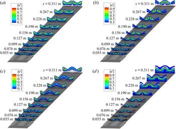
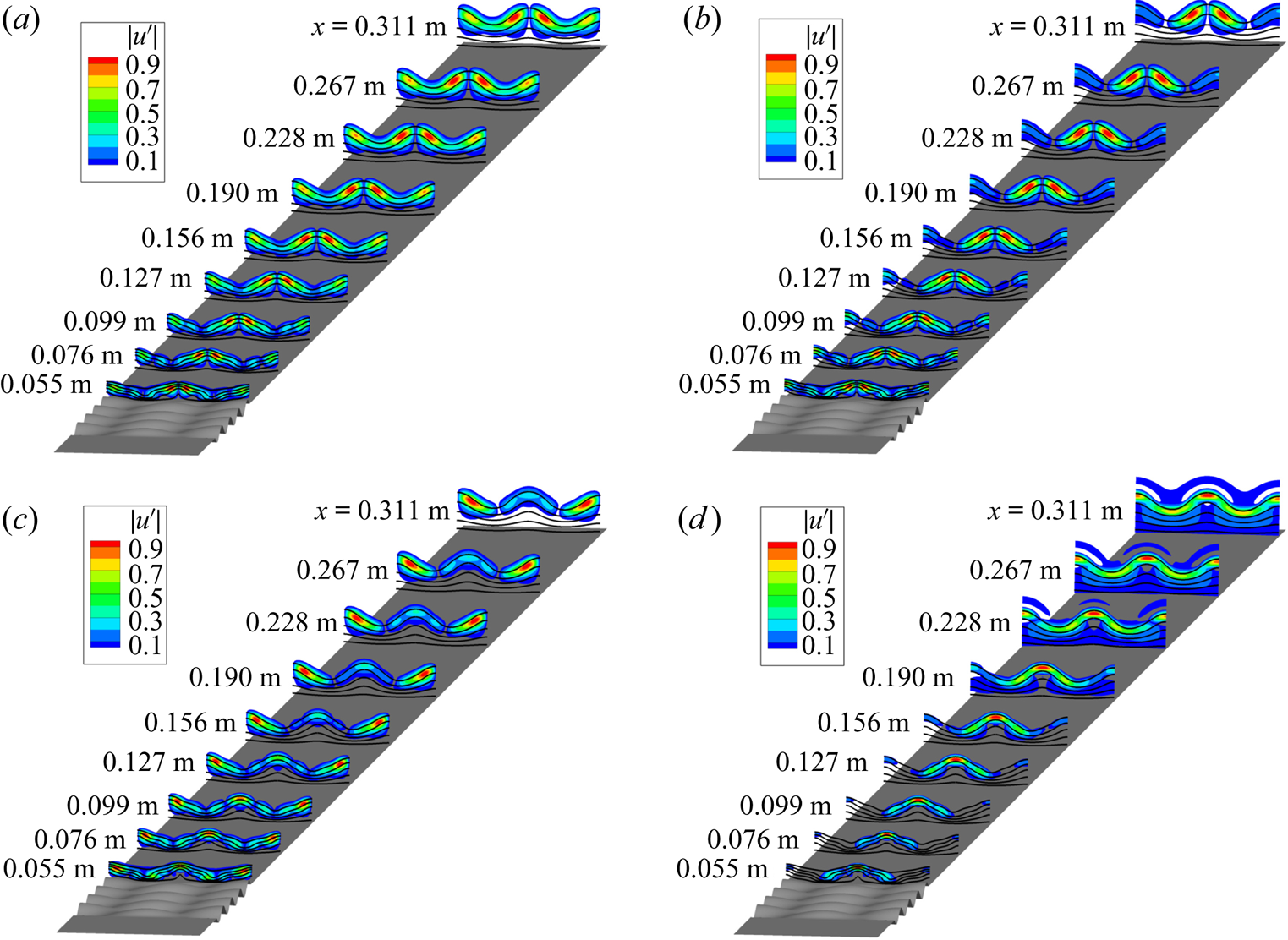
Several modes were identified in the wake of the roughness patch, which contained four roughness wavelengths in the streamwise direction and were given periodic boundary conditions in the spanwise direction. The modes in the wake of the roughness patch were identified as two different spanwise subharmonics of the antisymmetric mode (AS and SA), a fundamental antisymmetric mode (AA) and a fundamental symmetric mode (SS). These mode shapes are shown in figure 1 using contours of a non-dimensional streamwise velocity magnitude fluctuation  $(|u'| = \sqrt {\mathrm {Re}(u')^{2} + \mathrm {Im}(u')^{2}})$, normalized by its maximum at each streamwise station
 $|u'|_{max}$. The antisymmetric modes exhibit peaks of the
 $|u'|$ around both sides of either the symmetry boundaries of
 $z = 0$ or
 $\pm \lambda _z/2$ and the symmetric modes exhibit peaks of the
 $|u'|$ at the symmetry boundary (either
 $z = 0$ or
 $\pm \lambda _z/2$).
Mode shapes of normalized streamwise velocity fluctuation ( $|u'|$) associated with dominant instability modes from various families: (a) AA mode at
 $f = 50$ kHz; (b) SA mode at
 $f = 50$ kHz; (c) AS mode at
 $f = 50$ kHz; (d) SS mode at
 $f = 100$ kHz. Perspective is modified in order to view the mode shapes more clearly. Roughness patch parameters correspond to
 $k = 240\,{\rm \mu}{\rm m}$,
 $Re = 10.8 \times 10^{6}\,{\rm m}^{-1}$,
 $M = 3.5$ (reprinted with permission from Choudhari et al. (Reference Choudhari, Li and Paredes2018), figure 9). Flow from bottom to top.
The most-amplified mode was the AA mode, which occurred at a frequency ( $f$) of approximately 50 kHz for a free stream unit Reynolds number (
 $Re$) of
 $10.8 \times 10^{6}\,{\rm m}^{-1}$ and roughness height amplitude (
 $k$) of 240
 ${\rm \mu}{\rm m}$. The AA mode is characterized by an antisymmetric mode centred on the regions directly downstream of all locations where there was a protuberance or a dimple in the first row of the roughness pattern. The AS mode has an antisymmetric
 $u'$ distribution with respect to the spanwise location of the dimple in the first row of the roughness patch and a symmetric distribution centred over the regions downstream of where the first row in the roughness patch has a protuberance. The SA mode is similar to the AS mode, except that it has a symmetric
 $u'$ distribution with respect to the spanwise location of the dimple in the first row of the roughness patch and an antisymmetric distribution centred over the regions downstream of where the first row in the roughness patch has a protuberance. The SS mode has a symmetric spanwise distribution of
 $u'$ with respect to the locations of both where there was a protuberance or a dimple in the first row of the roughness pattern.
Further computational studies were performed using DNS to determine the evolution of disturbances over the roughness patch (Choudhari et al. Reference Choudhari, Li, Paredes and Duan2019). These computations showed the presence of some low-frequency disturbances, which, without the presence of the roughness patch, would not grow large enough to cause transition in a low-noise environment such as a quiet tunnel. The overall  $N$ factor of these low-frequency disturbances in the range of 30–100 kHz increased by 3.6 beyond those predicted by instability analysis of the 50 kHz wake instability alone.
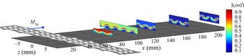
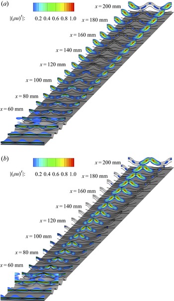
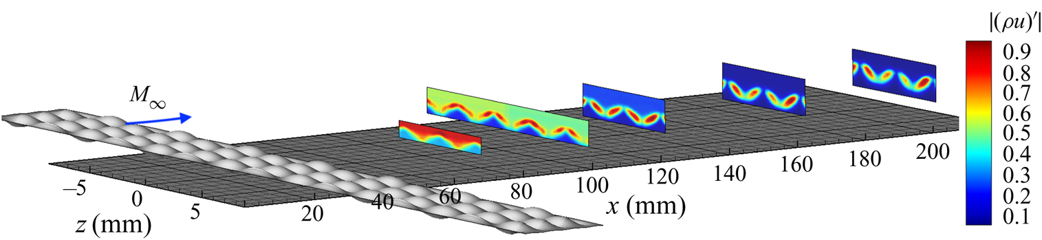
An experiment to complement these computations was conducted using hot-wire measurements of mass-flux fluctuations in the wake of the roughness elements. Details on the experiment can be found in the work by Chou, Kegerise & King (Reference Chou, Kegerise and King2020a). While the physical model used in the experiments could only accommodate 3.5 streamwise wavelengths ( $L_x/\lambda _x$), the measurements showed the presence of the AA mode dominated in the wake of the roughness patch. Figure 2 shows the contours of a non-dimensional mass flux
 $|(\rho u)'|$, which is given by the local mass-flux fluctuation normalized by the maximum mass-flux fluctuation in a given streamwise station
 $x$.
Mode shapes of mass-flux fluctuations  $|(\rho u)'|$ centred in a 5 kHz band around 55 kHz for
 ${k = 272\,{\rm \mu}{\rm m}}$ and
 $L_x/\lambda _x = 3.5$,
 $Re = 10.8\times 10^{6}\,{\rm m}^{-1}$,
 $M = 3.5$. The
 $x$ dimension is a different scale than the
 $y$ and
 $z$ dimensions to fit all of the mode shapes on the same page (redrawn from Chou et al. (Reference Chou, Kegerise and King2020a), figure 11). Flow from left to right.
Transition was not observed at this Reynolds number in the experiment of Chou et al. (Reference Chou, Kegerise and King2020a), so this experiment was repeated at a higher free stream unit Reynolds number. The present paper first discusses the experimental set-up of the measurements at a higher Reynolds number and the computational set-up of the basic state and stability analysis for an egg-crate roughness with the same number of streamwise wavelengths as the experiment. The experimental set-up involves detailed measurements in the wake of the roughness pattern with a hot wire. Due to the expense of the DNS, the stability analysis is conducted using a combination of the PSE and harmonic linearized Navier–Stokes equations (HLNSE). Next, the results of the measurements and the computations are presented and a comparison between the experimental and computational results are made. Finally, the experimental measurements and the computations are compared and the implications of the results are discussed.
3. Experimental set-up
3.1. Facility
Measurements were made in the NASA Langley Research Center Supersonic Low Disturbance Tunnel (SLDT), a Mach-3.5 quiet facility. A two-dimensional nozzle with exit dimensions of 15.24 cm by 25.40 cm (6 in. by 10 in.) was installed in the facility. Measurements of the free stream mass-flux fluctuations ( $(\rho u)'$) in an empty tunnel were made with a single normal hot wire and a constant-temperature anemometer. This hot wire was a platinum-plated tungsten wire that was 5
 ${\rm \mu}{\rm m}$ in diameter and approximately 1 mm long. These measurements were made with a symmetric bridge and an overheat ratio of 0.75 to be primarily sensitive to mass flux. The signals were sampled at 500 kHz for 2 s after passing through a signal conditioner with a high-pass filter cutoff at 100 Hz and a low-pass filter cutoff at 200 kHz. Mean measurements of the hot-wire voltage were recorded with a digital voltmeter.
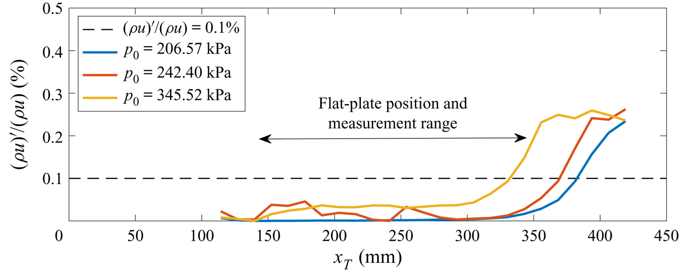
The data shown in figure 3 correspond to the hot-wire measurements that were made along the centreline of the two-dimensional nozzle in SLDT. These data are plotted against  $x_T$, which is the streamwise distance from the nozzle throat. The normalized root mean square (r.m.s.) mass-flux fluctuations between 100 Hz and 200 kHz are plotted as lines in the figure and a dashed line at 0.1 % indicates the threshold above which the flow is no longer considered to be ‘quiet’, based on previous definitions of the quiet core made by Beckwith et al. (Reference Beckwith, Creel, Chen and Kendall1983). As the stagnation pressure increases, the location where increased free stream fluctuations are greater than 0.1 % moves upstream. Within the
 ${\pm }10$ mm of the spanwise direction in the tunnel, the r.m.s. mass-flux fluctuations vary less than 2 % of the mean r.m.s., consistent with historic data from Chen, Malik & Beckwith (Reference Chen, Malik and Beckwith1989) for this facility.
Free stream mass-flux fluctuations along the tunnel centreline as measured with a hot wire for  $T_0 = 319.3\,{\rm K}$.
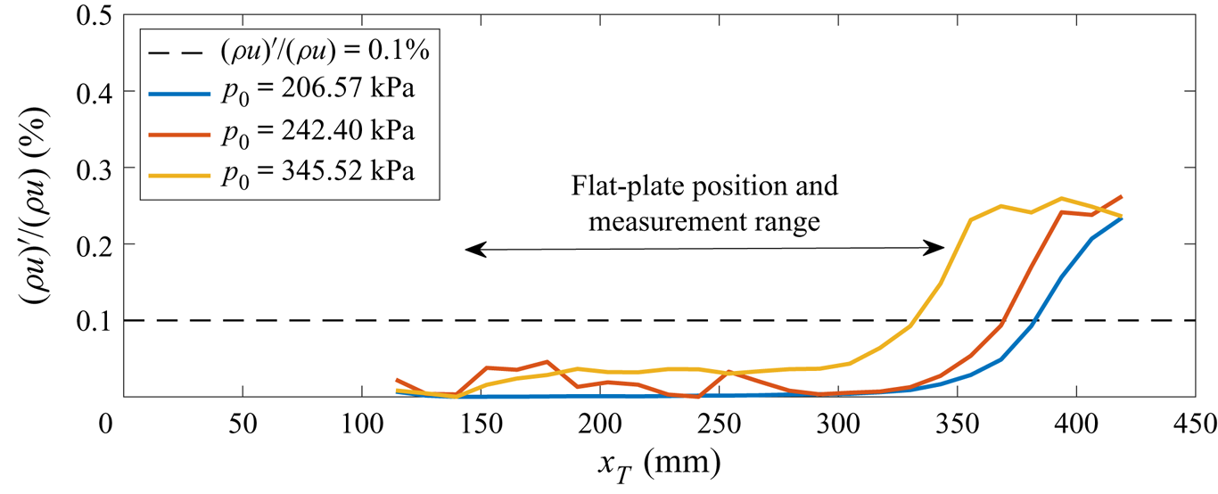
As mentioned previously, transition was not observed at the free stream unit Reynolds number of  $10.8\times 10^{6}\,{\rm m}^{-1}$ in figure 2, so the stagnation pressure was increased to approximately
 $241.7\pm 0.5$ kPa and the stagnation temperature (
 $T_0$) was held at the same temperature of
 $319.2\pm 0.2$ K. This condition corresponds to a free stream unit Reynolds number of approximately
 $12.6\times 10^{6}\,{\rm m}^{-1}$. The quiet uniform test core of the facility at these conditions extends from approximately
 $x_T = 125$ mm, where mean measurements show that flow uniformity begins, to approximately
 $x_T = 368.3$ mm, where the free stream fluctuations exceed 0.1 %. The flat plate model used for this experiment was positioned so that the following measurements made were within this region, illustrated in figure 3 by the double arrow.
3.2. Flat plate model and roughness pattern
The stainless-steel flat plate model was positioned so that the leading edge of the plate is  $x_T = 140$ mm from the nozzle throat, 15 mm downstream of the onset of uniform flow. Streamwise stations along the surface of the flat plate are denoted by
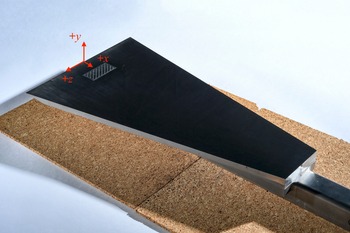
 $x$ and the coordinate system used for the flat plate measurements are given in figure 4, where a photograph of the flat plate model with the egg-crate roughness is shown. At
 $Re =12.6\times 10^{6}\,{\rm m}^{-1}$, the measurements extended to a streamwise station of
 $x = 206$ mm, which is approximately 22.5 mm forward of the end of the quiet core at this Reynolds number. The upper surface of the plate, where measurements are made, is polished to less than 0.1
 ${\rm \mu}$m r.m.s. roughness. The flat plate is 228.6 mm wide at the leading edge, with a leading edge thickness of between 76–127
 ${\rm \mu}$m. The flat plate is 406.4 mm long and tapers down to a width of 76.2 mm at the trailing edge to reduce the effects of corner and sidewall contamination.
Photograph of the polished flat plate with the egg-crate roughness insert installed, with the coordinate system labelled in red. Flow travels from the top left-hand corner towards the bottom right-hand corner, in the  $+x$ direction.
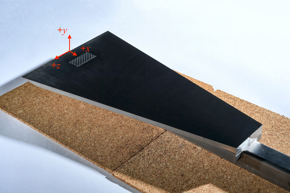
An egg-crate roughness pattern was cut into a stainless-steel insert that could be mounted into the flat plate model. The inserts are 25.4 mm by 50.8 mm in size and contain a flat border that was meant to sit flush to the flat plate model. The egg-crate roughness pattern was defined by an analytic function and the edges were modified using a Gaussian error function in a 1.588 mm border around the roughness pattern to transition to the flat surface. The vertical dimension of the egg-crate roughness pattern was defined similarly to the pattern defined in Choudhari et al. (Reference Choudhari, Li and Paredes2018) and Muppidi & Mahesh (Reference Muppidi and Mahesh2012),
 \begin{equation} h_w = k \sin \frac{2{\rm \pi} (x-x_0)}{\lambda_x} \cos \frac{2{\rm \pi} z}{\lambda_z}, \end{equation}
where  $x_0 = 28.8$ mm is the location of the leading edge of the insert relative to the leading edge of the flat plate,
 $k = 272\,{\rm \mu}{\rm m}$ is the roughness height amplitude and
 $\lambda _x = \lambda _z = 6.25$ mm are the streamwise and spanwise wavelengths, respectively. The sinusoidal form was modified with a Gaussian error function used to taper the edges of the pattern defined by
 \begin{equation}
h_{taper} = \begin{cases} \dfrac{1}{2}\left(1 +
\dfrac{2}{\sqrt{\rm \pi}} \displaystyle\int_0^{x-x_0-x_{taper}}
e^{{-}t^{2}} \,{\rm d}t \right) & \text{if } x-x_0 \leq
L_x/2,\\
\dfrac{1}{2}\left(1 + \dfrac{2}{\sqrt{\rm \pi}}
\displaystyle\int_0^{L_x-x_{taper}-x} {\rm e}^{{-}t^{2}} \,{\rm d}t
\right) & \text{if } x-x_0 \geq L_x/2,\\
\dfrac{1}{2}\left(1 + \dfrac{2}{\sqrt{\rm \pi}}
\displaystyle\int_0^{z+L_z/2-x_{taper}} {\rm e}^{{-}t^{2}} \,{\rm d}t
\right) & \text{if } z \leq 0,\\
\dfrac{1}{2}\left(1 + \dfrac{2}{\sqrt{\rm \pi}} \displaystyle\int_0^{L_z/2-x_{taper}-z} {\rm
e}^{{-}t^{2}} \,{\rm d}t \right) & \text{if } z \geq 0,\\
1 & \text{otherwise}, \end{cases}
\end{equation}
where  $x_{taper}$ is the tapering length of 1.588 mm,
 $L_x =25.4$ mm is the streamwise dimension of the insert and
 $L_z = 50.8$ mm is the spanwise dimension of the insert. The specified shape of the roughness insert was given by
 $h_{nominal} = h_w \, h_{taper}$.
The leading edge of the insert is located at  $x = 28.8$ mm and the first row of protuberances is centred near
 $x = 32.0$ mm. Using a compressible flat-plate boundary-layer code to compute the boundary layer thickness based on 99.5 % of the edge velocity, the unperturbed flat plate boundary layer thickness is nominally 0.56 mm at the location of the first row of protuberances at a unit Reynolds number of
 $12.6\times 10^{6}\,{\rm m}^{-1}$. Using the computed unperturbed boundary layer thickness at this location, the ratio of roughness height to boundary layer thickness (
 $k/\delta$) is approximately 0.49. At the start of the roughness insert, the computed
 $N$ factor envelope of the boundary layer with no roughness has a value of 1.2.
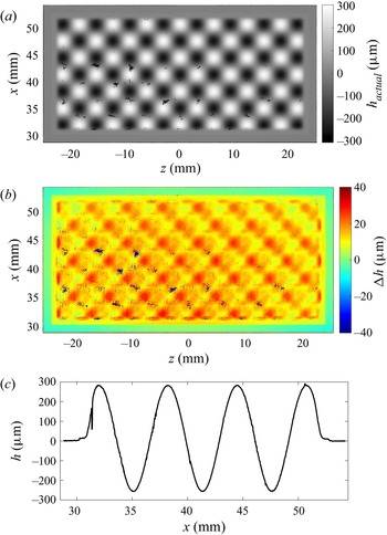
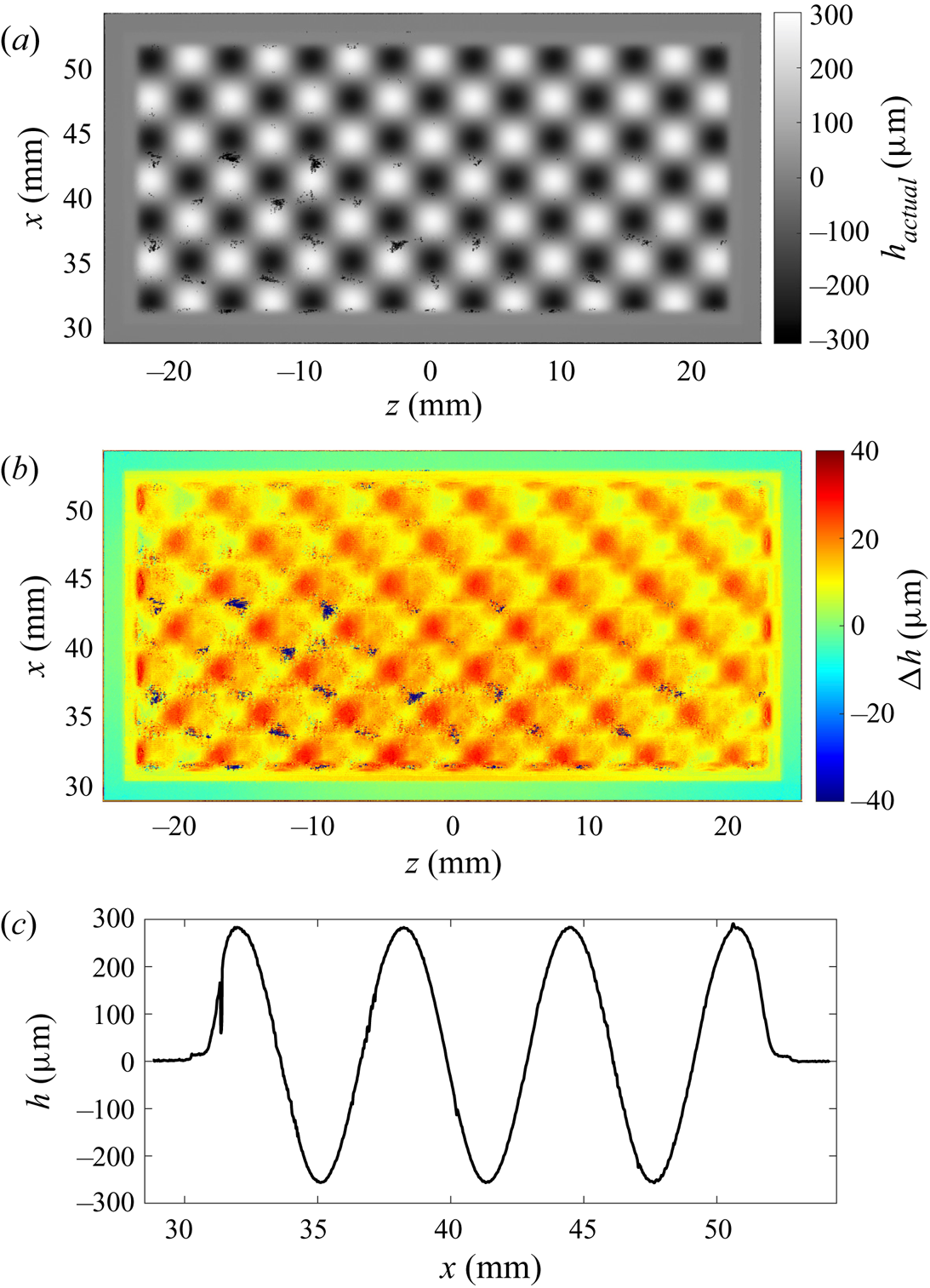
A three-dimensional scanning measurement system was used to determine how closely the roughness insert matched the computer-aided design (CAD) model defined by  $h_{nominal}$. The scan of the egg-crate roughness insert is shown in figure 5(a) and the difference between the measured surface and the CAD model
 $(\Delta h = h_{actual} - h_{nominal})$ is shown in figure 5(b). Regions of measurement dropout are given by patches of black in the images. At most, there is a 5–10
 ${\rm \mu}{\rm m}$ vertical offset between the tapered egg-crate roughness pattern and the machined flat border of the insert. An example of the vertical offset is shown in figure 5(c), which shows a line cut along the centreline in the streamwise direction and a slight step at the front and back of the roughness pattern near
 $x = 30$ mm and 52 mm. This offset at the tapered edge causes the average protuberance height to be approximately 303.9
 ${\rm \mu}{\rm m}$ tall and the average dimple depth to be approximately 239.3
 ${\rm \mu}{\rm m}$ deep relative to the flat plate surface.
Measurements of the egg-crate roughness with comparator: (a) of surface height  $h$; (b) the difference between analytic function and measurement
 $\Delta h$; and (c) a line cut down the centreline of the egg-crate roughness measurement in the streamwise direction.
Measurements were acquired around the installed insert to see if there were any significant steps between the machined flat border of the insert and the flat-plate surface. A surface contact profilometer was used to measure the step at several discrete locations around the insert. These measurements were taken in the streamwise direction at the front corners and a random location along the leading edge of the insert as well as the back corners and along a random location at the back of the insert. The step height between the flat plate surface and the flat border of the insert was no more than 3  ${\rm \mu}{\rm m}$, i.e. within manufacturing tolerances. This was independently verified by using the three-dimensional scanning measurement system on a replicant mould of the installed insert.
3.3. Instrumentation
Hot-wire anemometry with the same anemometer and symmetric bridge as in the free stream measurements was used to probe the boundary layer. The sensing element for the boundary layer probes was a smaller 3.8  ${\rm \mu}{\rm m}$ platinum-plated tungsten wire with a nominal length of 0.5 mm. With the smaller sensing element, the maximum bandwidth of the hot-wire measurements increases to 370 kHz. The hot wire was set to a high overheat ratio of 0.75 in order to be primarily sensitive to mass flux while ensuring that the wire would not be subjected to temperatures higher than the oxidation temperature. The measurements were passed through a signal conditioner that had a high-pass filter cutoff at 100 Hz and a low-pass filter cutoff at 400 kHz. The signal was sampled at 1 MHz for 1 s at each measurement location. The cold wire resistance was also measured at each measurement station to correct for the total temperature change in the boundary layer. Calibration of the hot wire was performed as in Kegerise et al. (Reference Kegerise, Owens and King2010) and the uncertainty of the calibration based on the mean-squared error is, at most, 6.0 % of the mean. Kegerise et al. (Reference Kegerise, Owens and King2010) evaluated the effect of the probe body on the mean-flow distortion with computational fluid dynamics (CFD) simulations and showed that the worst-case mass-flux uncertainty was approximately 2 % due to probe interference.
4. Computational set-up
In this section, the methodology used for the analysis of the disturbance amplification over the flat plate with the roughness patch is presented. The laminar boundary layer solution is based on the full Navier–Stokes equations. The evolution of convective instabilities is calculated with the linear plane-marching PSE and the HLNSE frameworks.
4.1. Laminar boundary layer flow
The CFD code ‘viscous upwind algorithm for complex flow analysis’ (VULCAN-CFD) (Baurle et al. Reference Baurle, White, Drozda and Norris2020) was used to compute the unperturbed, two-dimensional boundary layer flow over the flat plate without the roughness patch, but including the leading edge and bow shock. This code solves the unsteady conservation equations for laminar or turbulent flow of calorically or thermally perfect gases with a spatially second-order accurate cell-centred finite-volume scheme. The VULCAN-CFD computation used inviscid fluxes constructed with the ‘monotonic upstream-centred scheme for conservation laws’ (MUSCL)  $\kappa = 0$ scheme, the van Albada gradient limiter (van Albada, van Leer & Robers Reference van Albada, van Leer and Robers1982), and the ‘low dissipation flux split scheme’ (LDFSS) of Edwards (Reference Edwards1997).
The two-dimensional solution was used as the inflow condition to compute the three-dimensional, laminar boundary layer flow over the flat plate with the egg-crate roughness patch with a high-order DNS solver. A detailed description of the governing equations and their numerical solution is given by Wu & Martin (Reference Wu and Martin2007). The inviscid fluxes from the governing equations are computed using a seventh-order weighted essentially non-oscillatory (WENO) finite-difference scheme introduced by Jiang & Shu (Reference Jiang and Shu1996); the present scheme also allows the use of limiters that have been optimized to reduce the numerical dissipation. Both an absolute limiter on the WENO smoothness measurement and a relative limiter on the total variation are employed simultaneously during the simulation. The viscous fluxes are discretized using a fourth-order central difference scheme and time-accurate integration is performed using a third-order low-storage Runge–Kutta scheme (Williamson Reference Williamson1980).
The three-dimensional computational domain was discretized with 1200 points in the streamwise direction, 80 points in the spanwise direction and 240 points in the wall-normal direction. A periodic boundary condition was imposed in the spanwise direction with a domain length equal to a wavelength of the roughness geometry. Grid resolution was examined as described in Choudhari et al. (Reference Choudhari, Li, Paredes and Duan2019).
4.2. Stability analysis
For the present flat-plate configuration, the Cartesian coordinates  $(x,y,z)$ correspond to the streamwise, wall-normal and spanwise coordinates, respectively, and the vector
 $(u, v, w)$ represents the corresponding velocity components. A curvilinear, non-orthogonal transformation of the grid is performed along the roughness patch. Density and temperature are denoted by
 $\rho$ and
 $T$, respectively.
The vector of perturbation variables is denoted by  $\tilde {\boldsymbol {q}}(x,y,z,t)=(\tilde {\rho },\tilde {u},\tilde {v},\tilde {w},\tilde {T})^{\rm T}$ and the vector of disturbance functions is
 $\breve {\boldsymbol {q}}(x,y,z)=(\breve {\rho },\breve {u},\breve {v},\breve {w},\breve {T})^{\rm T}$. The vector of basic state variables is
 $\bar {\boldsymbol {q}}(x,y,z)=(\bar {\rho },\bar {u},\bar {v},\bar {w},{{\bar {T}}})^{\rm T}$. The linear perturbations are assumed to be harmonic in time and are written as
 \begin{equation} \tilde{\boldsymbol{q}}(x,y,z,t)=\breve{\boldsymbol{q}}(x,y,z) \exp\left(-{{\rm i}} \omega t\right)+{\rm c.c.}, \end{equation}
where the  $\omega$ is the angular frequency, and
 ${\rm c.c.}$ refers to the complex conjugate.
The disturbance functions  $\breve {\boldsymbol {q}}(x,y,z)$ satisfy the three-dimensional HLNSE (Paredes et al. Reference Paredes, Choudhari, Li, Jewell, Kimmel, Marineau and Grossir2019), where the linear operators depend on the basic state variables and parameters, and on the angular frequency of the perturbation,
 \begin{equation} \boldsymbol{\mathsf{L}}_{HLNSE}\breve{\boldsymbol{q}}(x,y,z)=\breve{\boldsymbol{f}}, \end{equation}
where  $\breve {\boldsymbol {f}}$ represents an inflow condition or forcing term.
The PSE approximation to the HLNSE is applicable along the wake of the roughness because the basic state variables vary slowly along the streamwise direction. The PSEs are based on isolating the rapid phase variations in the streamwise direction via the disturbance ansatz
 \begin{equation} \breve{\boldsymbol{q}}(x,y,z)=\hat{\boldsymbol{q}}(x,y,z) \exp\left[ {{\rm i}} \int_{x_0}^{x}\alpha(x')\,{\rm d} x'\right]. \end{equation}
The unknown streamwise varying wavenumber  $\alpha (x)$ is determined in the course of the solution by imposing an additional constraint
 \begin{equation} \int_z\int_y \hat{\boldsymbol{q}}^{*} \frac{\partial \hat{\boldsymbol{q}}}{\partial x}\,{\rm d} y\,{\rm d}z=0. \end{equation}
Hence, the amplitude functions  $\hat {\boldsymbol {q}}(x,y,z)=(\hat {\rho },\hat {u},\hat {v},\hat {w},\hat {T})^{\rm T}$ vary slowly in the streamwise direction in comparison with the phase term
 $\exp [ {{\rm i}} \int _{x_0}^{x}\alpha (x')\,{\rm d} x']$. Note that the amplitude function
 $\hat {\boldsymbol {q}}$ of (4.3) is three-dimensional because the present flow problem is inhomogeneous in the three spatial directions. Therefore, the conventional line-marching PSE that assumes homogeneous spanwise direction of the basic state and amplitude functions is not applicable, and the plane-marching PSE are used instead. Substituting (4.3) into the HLNSE and invoking scale separation between the streamwise coordinate and the other two directions to neglect the viscous terms with streamwise derivatives, the plane-marching PSE are obtained in the form
 \begin{equation} \left(\boldsymbol{\mathsf{L}}_{PSE}+\boldsymbol{\mathsf{M}}_{PSE}\frac{\partial}{\partial x}\right)\hat{\boldsymbol{q}}(x,y,z)=0, \end{equation}
where  $\boldsymbol{\mathsf{L}}_{PSE}$ indicate the linear operators of the plane-marching PSE and
 $\boldsymbol{\mathsf{M}}_{PSE}$ has the terms multiplying the first-order streamwise derivatives in the linearized Navier–Stokes equations (Paredes, Choudhari & Li Reference Paredes, Choudhari and Li2017).
The onset of laminar–turbulent transition is estimated by using the logarithmic amplification ratio, the so-called  $N$-factor, relative to the lower bound location
 $x_{I}$, where the disturbance first becomes unstable,
 \begin{equation} N_\phi={-}\int_{x_{I}}^{x}\alpha_i(x')\,\mathrm{d} x'+\ln\left[\hat{\phi}(x)/\hat{\phi}(x_{I})\right]. \end{equation}
Here,  $\hat {\phi }$ denotes an amplitude norm of
 $\hat {\boldsymbol {q}}$, e.g. the maximum mass-flux disturbance.
Traditionally, the instability of roughness elements has been studied by analysing the wake of the roughness elements with two-dimensional, quasiparallel eigenvalue analysis (e.g. Choudhari et al. Reference Choudhari, Li, Wu, Chang, Edwards, Kegerise and King2010, Reference Choudhari, Li, Chang, Norris and Edwards2013; Padilla Montero & Pinna Reference Padilla Montero and Pinna2021) or plane-marching PSE (e.g. De Tullio et al. Reference De Tullio, Paredes, Sandham and Theofilis2013; Choudhari et al. Reference Choudhari, Li and Paredes2018, Reference Choudhari, Li, Paredes and Duan2019). The plane-marching PSE calculation of the roughness wake instabilities initiated just downstream of the roughness patch is denoted as ‘PSE-only’ in the present paper.
Additionally, the integration of oblique, first-mode instabilities that begin to amplify upstream of the roughness patch for the present configuration, and continue to grow over and in the wake of the roughness patch is carried out by using a combination of the plane-marching PSE and HLNSE methods. First, the first-mode waves are integrated from their corresponding neutral locations, i.e. zero-growth-rate streamwise location by using the plane-marching PSE to account for the upstream influence of the roughness patch. Then, the amplitude function vector  $\hat {\boldsymbol {q}}$ from the plane-marching PSE solution at a streamwise location of
 $x=20$ mm is used as the inflow condition for the HLNSE calculation along the roughness patch. The plane-marching PSE are not able to capture the disturbance evolution over the roughness patch due to the strong streamwise gradients of the boundary-layer flow. Therefore, the HLNSE are required to calculate the evolution of the first-mode disturbances along the roughness patch. Finally, the plane-marching PSE are integrated along the wake of the roughness patch by using the solution of the HLNSE as the inflow condition at
 $x=60$ mm. This method is referred to in the remainder of this paper as ‘HLNSE+PSE.’ The three-dimensional HLNSE calculation of the instability waves along the roughness patch requires roughly two orders of magnitude more computational power than a plane-marching PSE calculation.
The plane-marching PSE are discretized with high-order finite-difference schemes (Hermanns & Hernández Reference Hermanns and Hernández2008; Paredes et al. Reference Paredes, Hermanns, Le Clainche and Theofilis2013) of sixth order for the cross-plane of spanwise and wall-normal coordinates with  $N_y=141$ and
 $N_z=65$ points, respectively. The PSE are integrated along the streamwise coordinate by using second-order backward differentiation and with enough grid points to ensure convergence of the results. The HLNSE are discretized with twelfth-order finite-difference schemes along the spanwise and wall-normal coordinates with
 $N_y=61$ and
 $N_z=49$, respectively. The streamwise coordinate is discretized with a fourth-order centred finite-difference scheme with
 $N_x=701$ points for a streamwise domain of
 $x\in [20, 65]$ mm. Because of the selected discretization scheme along
 $x$, the matrix
 $\boldsymbol{\mathsf{L}}_{HLNSE}$ of (4.2) becomes a block pentadiagonal matrix. The linear system is solved by using a combined multithread and multiprocessor algorithm based on Thomas’ algorithm and the dual Schur complement method (Carpenter et al. Reference Carpenter, Choudhari, Li, Streett and Chang2010). An interior plane of this solution at
 $x=60$ mm is used for the inflow of the plane-marching PSE in the wake of the roughness to exclude any effects of the outflow boundary condition on the HLNSE solution.
The plane-marching PSE and HLNSE use the same wall-normal and spanwise boundary conditions. The amplitude functions are forced to decay at the far-field boundary by imposing the Dirichlet conditions  $\hat {\rho }=\hat {u}=\hat {w}=\hat {T}=0$. The far-field boundary coordinate is set below the shock layer. Only one roughness wavelength
 $\lambda _z=6.25$ mm, which corresponds to the roughness spanwise wavenumber of
 $\beta _R=2{\rm \pi} /\lambda _z=1005.3\,{\rm m}^{-1}$, is discretized to exploit the symmetries of the flow. The selection of boundary conditions at both symmetry planes determines the nature of the instability mode and the spanwise disturbance wavelength. Table 1 shows the boundary conditions used in each case.
Spanwise boundary conditions used in the plane-marching PSE and HLNSE analyses. The mode labels AA, SS, SA and AS refer to antisymmetric and symmetric conditions at each boundary. Also, note that the subscript  $()_z$ is equivalent to
 $\partial ()/\partial z$.

The number of discretization points in all three directions and the streamwise and wall-normal domain size were varied to ensure that the relevant flow quantities were insensitive to further improvement in grid resolution and enlargement of the domain size.
5. Experimental results
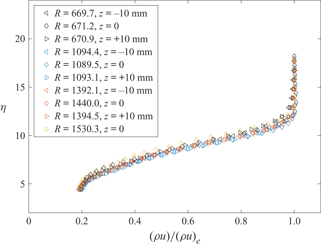
Baseline measurements of the flow without a roughness are provided in figure 6. These profiles are non-dimensionalized with the Blasius self-similarity parameter 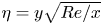 $\eta = y \sqrt {Re/x}$ for the height above the surface and with the parameter
 $R = \sqrt {Re\, x}$ for the streamwise distance. These boundary layer profiles were used to check the uniformity of the clean flat-plate boundary layer. The measurements shown in figure 6 were made prior to the installation of the roughness pattern. The excellent self-similarity of the profiles, regardless of streamwise or spanwise location, shows that there is negligible yaw or angle of attack in the installation of the flat plate. Once the egg-crate roughness insert was installed in the flat plate, no further installation or polishing of the surface of the flat plate was required. No measurable instabilities were observed in these boundary layer profiles, which is expected because the maximum
 $N$ factor at the farthest downstream measurement station is 4.4.
Boundary layer profiles on a flat plate with no roughness at several stations in the streamwise and spanwise extent of the measurement region.

5.1. Mean measurements
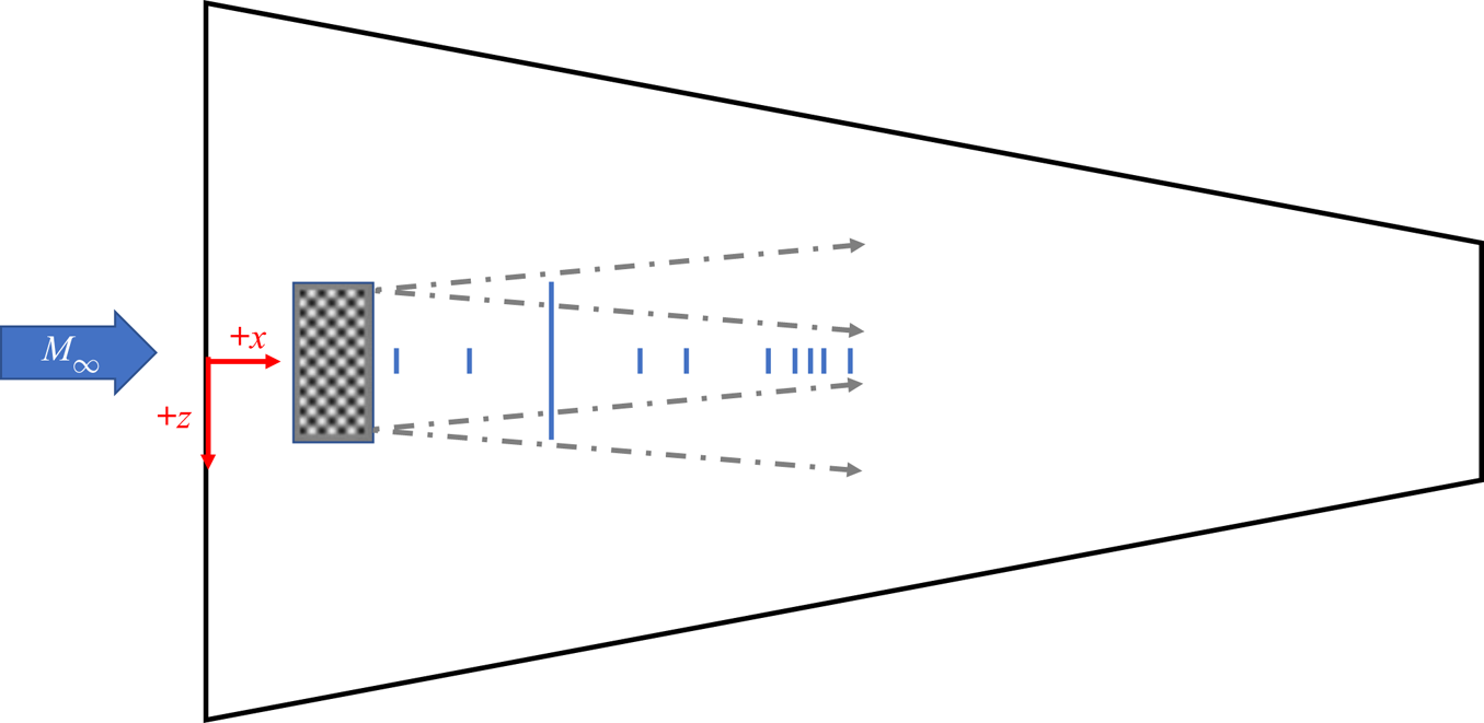
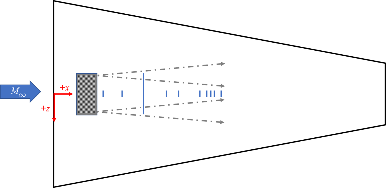
Measurements of the wake of the roughness were made at locations indicated by the blue line in figure 7. The diagram is drawn to scale, with notional locations of the possible contamination lines from the roughness insert given by the dashed arrows. Measurements of the mean mass flux ( $\rho u$) were taken with a hot-wire probe at several locations downstream of the egg-crate roughness. Data were collected as a series of spanwise profiles at several heights above the wall. Almost all of the spanwise cross-sectional surveys have measurements spaced 0.2 mm apart in the spanwise (
 $z$) direction and at least 16 points in the vertical (
 $y$) direction. Several streamwise (
 $x$) stations were selected to perform a survey of the
 $yz$-planes downstream of the roughness patch.
Scale diagram of the flat plate with measurement locations marked by blue lines. Dashed arrows indicate possible contamination lines from edges of insert. Coordinate system labelled in red, with the  $+y$ direction coming out of the page.
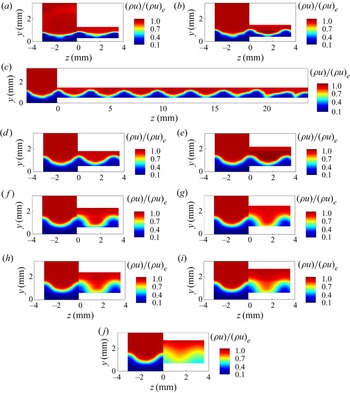
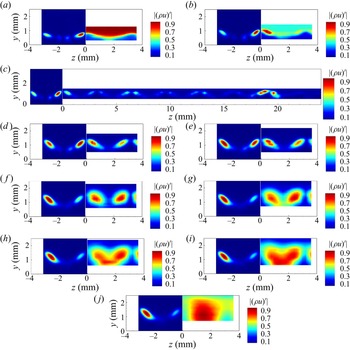
The measured mean mass-flux contours for multiple streamwise stations are provided in figure 8 on the right-hand side of each contour plot, where they have been normalized by the edge mass-flux ( $(\rho u)_e$). The laminar solution of the time-accurate DNS for the same configuration are provided on the left-hand side of each contour plot.
Mean mass-flux contours behind the egg-crate roughness for the measurement plane located at multiple streamwise stations:  $M = 3.5$;
 $Re = 12.6\times 10^{6}\,{\rm m}^{-1}$. Measurements from the experiment are given on the
 $+z$ side of the figures and the time-accurate laminar solution for the DNS is given on the
 $-z$ side of the figures for comparison: (a)
 $x = 58.8$ mm; (b)
 $x = 84.7$ mm; (c)
 $x = 110.6$ mm; (d)
 $x = 138.4$ mm;(e)
 $x = 153.8$ mm; ( f)
 $x = 179.7$ mm; (g)
 $x = 188.3$ mm; (h)
 $x = 192.7$ mm; (i)
 $x = 197.0$ mm; (j)
 $x = 205.6$ mm.

The mean mass-flux contours illustrate the mean-flow distortion present in the boundary layer downstream of the roughness elements. Most of the measurements at each streamwise station span  $\pm 3.6$ mm across the centreline, approximately one wavelength of the egg-crate roughness pattern and two wavelengths of the mean flow distortion. A single spanwise cross-sectional survey extending approximately
 ${\pm }24$ mm across the span of the plate on either side of the centreline was also made to determine if end effects would be expected near the centre of the flat plate. Wider spanwise measurements were not possible at farther downstream stations due to physical constraints of the facility and existing equipment. The measurements presented in figure 9 provide some indication of the repeatability of the mean flow measurements. The measurements were made on different days over several months spanning the beginning and end of the experiment.
Mean mass-flux contours at  $x = 110.6$ mm.

End effects are seen starting near  $z = \pm 18.5$ mm in the measurements at
 $x = 110.6$ mm in figure 9. Using this location and a conservative assumption that the disturbances originate from the downstream corner of the roughness insert, a spreading angle of 7
 $^{\circ }$ is inferred. The end effects should not be seen at least between a region of approximately
 ${\pm }6.4$ mm on either side of the centreline at the farthest downstream measurement station of
 $x = 205.6$ mm. Thus, the focus of the remainder of the measurements along
 $\pm 3.6$ mm of the centreline of the flat plate without considering spanwise end effects of the finite roughness patch is justified.
At locations of  $x = 153.8$ mm and farther upstream (figure 9a–e), periodic distortion of the mean flow is observed across the span of the wake, with the peaks and troughs of the distortion centred behind the protuberances and dimples of the roughness pattern. The measurements of the mean mass flux are similar to each other at these streamwise stations, but become dissimilar starting near
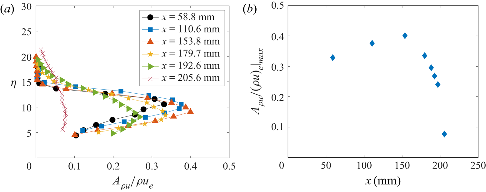
 $x = 179.7$ mm. The mean flow distortion is more quantitatively observed via the streak strength profile, which can be defined as
 \begin{equation} A_{\rho u} = \frac{1}{2} \left(\rho u\left(y\right)_{high} - \rho u\left(y\right)_{low} \right), \end{equation}
where  $\rho u(y)_{high}$ is defined as the maximum mass flux at each
 $y$ location and
 $\rho u(y)_{low}$ is the corresponding minimum mass flux. The streak amplitude
 $A_{\rho u}/(\rho u)_e|_{max}$ is defined as the wall-normal maximum of the streak strength profile. Figure 10(a) shows the streak strength profiles at each
 $x$ station shown in figure 8, and figure 10(b) indicates the streak amplitude at each of the streamwise stations. The streak amplitude increases and then begins to decrease somewhere upstream of
 $x = 179.7$ mm, and the streak strength profile becomes fairly constant across the boundary layer at
 $x = 205.6$ mm, the farthest downstream station where measurements were made. Further indication of the breakdown of this flow to turbulence is provided in the next section, where the power spectra are examined.
(a) Streak strength profiles at each streamwise station and (b) streak amplitude over the measurement region.

5.2. Power spectra
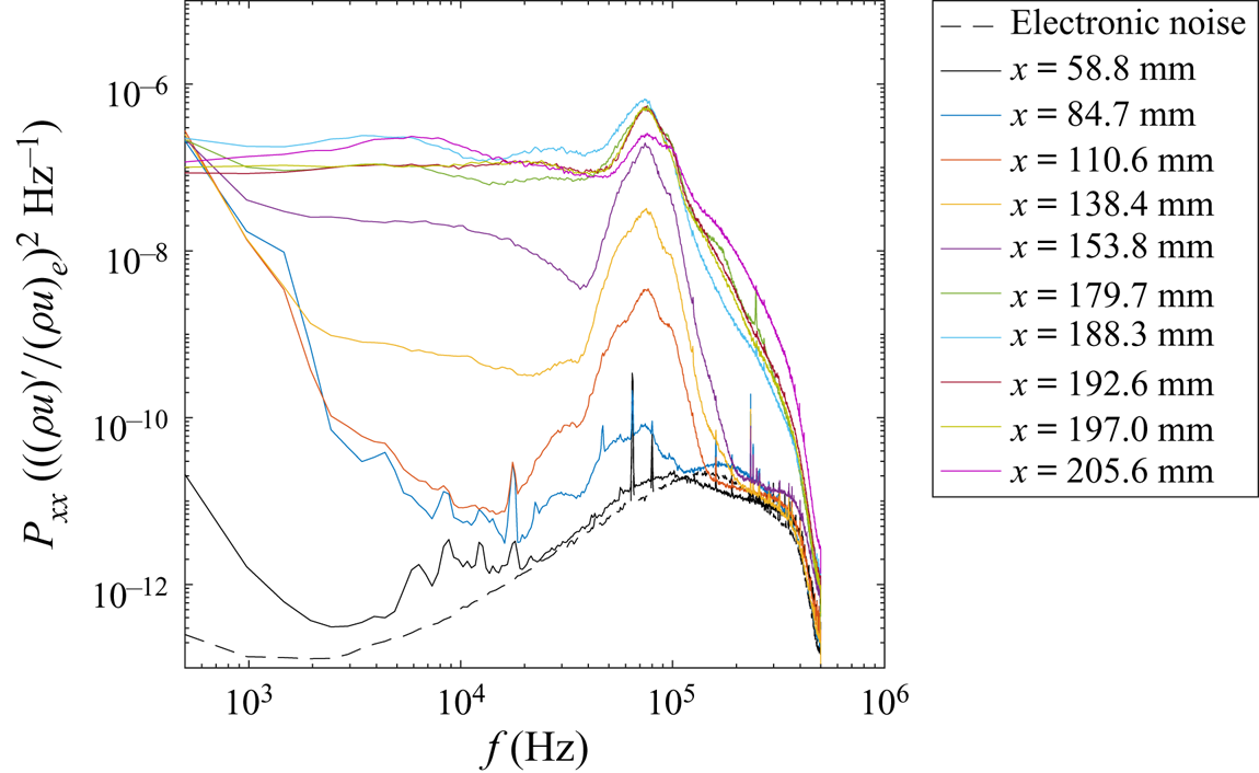
Power spectra of the mass-flux fluctuations were calculated using Welch's spectrum estimation method, using Hann windows of 2048 points and 50 % data overlap. These parameters yielded a frequency resolution of 488.3 Hz for the spectra computed. At each  $x$-station, the location between
 $z = -0.2$ and 1.5 mm with the highest broadband r.m.s. fluctuations was selected to monitor the growth of the disturbances near the centreline of the wake of the roughness patch. This smaller region was selected as an objective method of searching for a maximum r.m.s. in the fluctuations, particularly in regions where there was low signal relative to the electronic noise floor. The spanwise region was selected to allow for the possibility of finding both symmetric and antisymmetric disturbances near the centreline. Likewise, no bounds were placed on the vertical location of the maximum r.m.s. fluctuation to allow for the search region to change with the growing boundary layer thickness. The
 $+z$ side of the spanwise cross-sectional survey was selected to attempt to follow the same disturbance structure at each streamwise measurement station.
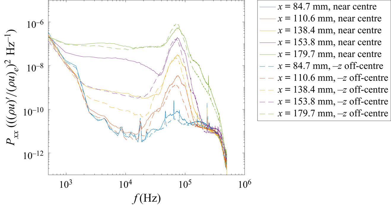
Figure 11 shows the power spectra at locations where the largest r.m.s. amplitude was found in the search region at each  $x$ station. Generally, these large r.m.s. amplitudes occurred near
 $z = 0.5$ mm,
 $y = 1.2$ mm. A large peak near 75 kHz appears in the spectra starting near
 $x = 84.7$ mm and grows in amplitude with downstream distance. At farther downstream stations, starting at approximately
 $x = 179.7$ mm, the peak in the spectra remains approximately the same amplitude, but the power in the lower frequencies increases. The peak at 75 kHz suddenly decreases in amplitude between
 $x = 192.6$ mm and 205.6 mm, and the spectral power across the other frequencies below 100 kHz is relatively flat, suggesting that the flow is near the end of transition.
Power spectra taken at the location with the largest r.m.s. near the centreline for the most-amplified disturbance in a planar survey. The electronic noise floor of the system is also shown.

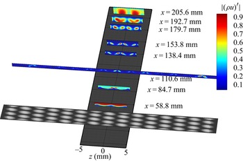
To visualize the mode shapes in the wake of the roughness, the r.m.s. amplitude of the fluctuations centred near 75 kHz was computed by integrating the power spectra in a 5 kHz bandwidth centred around this frequency and taking the square root. The r.m.s. amplitude in this bandwidth was then normalized by the maximum r.m.s. amplitude of the measurements at each  $x$ location to achieve a peak amplitude of unity. These data were captured in a contour plot to better understand the evolution of the disturbances in the wake of the roughness element in figure 12.
The r.m.s. mass-flux fluctuation contours for the 75 kHz instability behind the egg-crate roughness for the measurement plane located at multiple streamwise stations:  $M = 3.5$;
 $Re = 12.6\times 10^{6}\,{\rm m}^{-1}$. Flow travels from bottom to top of image.

At  $x = 58.8$ mm, the measurements are barely above the electronic noise and show no clear disturbance peaks. At
 $x = 84.7$ mm, the antisymmetric mode appears along the centreline wake (
 $-1.6\,{\rm mm} < z < 1.6\,{\rm mm}$) of the roughness pattern. At farther downstream stations, an antisymmetric mode also appears in the off-centreline wakes (
 $-4.8\,{\rm mm} < z < -1.6\,{\rm mm}$ and
 $1.6\,{\rm mm} < z < 4.8\,{\rm mm}$). The contours of the r.m.s. fluctuations centred near 75 kHz are shown to be antisymmetric across the span, which resembles the AA mode.
Upstream of  $x = 179.7$ mm the centreline antisymmetric mode has a higher amplitude than the off-centreline antisymmetric modes. At
 $x = 179.7$ mm, the off-centreline antisymmetric modes begin to have a higher amplitude than the centreline antisymmetric modes. The mode shapes at this location also begin to look distorted and display spatial spreading, likely indicating nonlinear interaction and/or the beginning of breakdown into turbulence. As the flow breaks down, the disturbances in the off-centreline wakes centred near
 $z = \pm 2.4$ mm begin to merge with the disturbances in the centreline wake centred near
 $z = \pm 0.8$ mm. At the farthest downstream measurement station of
 $x = 205.6$ mm, the antisymmetric disturbances in the wake merge with the adjacent antisymmetric disturbances into a region of high-amplitude fluctuations centred at
 $z = {\pm }1.6$ mm.
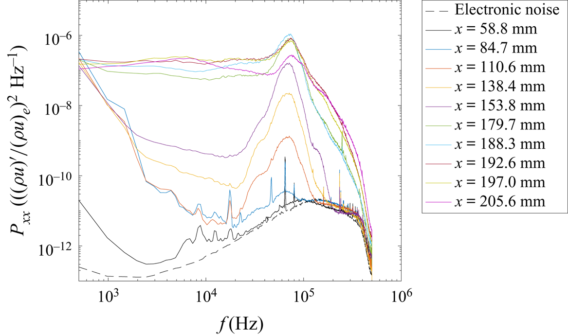
The change in amplitude between the instabilities in the centreline wake and the off-centreline wake can also be captured in the power spectra. As an example, figure 13 shows the power spectra of the off-centreline disturbances growing near  $z=-2.6$ mm,
 $y = 1.1$ mm at several streamwise stations. In this region, the frequency with the most spectral power appears to be located closer to 70 kHz rather than 75 kHz. The growth of this peak is fairly similar to the instability in the wake of the centreline protuberances, shown in figure 11. However, the low-frequency content between 2 and 20 kHz appears to grow more slowly for the off-centreline disturbances than for the on-centreline disturbances, particularly between streamwise stations of
 $x = 110.6$ mm and 153.8 mm.
Power spectra taken at the location with the largest r.m.s. in the wake of the protuberances centred near  $z= -2.6$ mm.

A direct comparison of the spectra between streamwise stations of  $x = 84.7$ mm and
 $x = 179.7$ mm is provided in figure 14. The spectra near
 $z = 0.5$ mm and
 $y = 1.2$ mm (centreline wake) are given by the solid lines and the spectra of the fluctuations near
 $z = -2.6$ mm and
 $y = 1.1$ mm (off-centreline wake) are given by the dashed lines. At
 $x = 84.7$ mm, the initial amplitude of the instability in the off-centreline wake appears smaller than the instability in the centreline wake. However, at
 $x = 138.4$ mm, the spectral amplitude of the dominant instability is approximately equal for both the centreline and off-centreline wakes. The largest difference between the centreline wake and the off-centreline wake is the low-frequency content below 20 kHz, which grows more rapidly between
 $x = 110.6$ mm and 153.8 mm for the wake on the centreline than the off-centreline wake. This low-frequency content is approximately equal by
 $x = 179.7$ mm. The higher amplitudes of the instability in the centreline wake indicate that it is more likely to reach nonlinear amplitudes earlier than the off-centreline instability.
Comparison of power spectra in the wake of the protuberances centred near  $z= -2.6$ mm to the power spectra in the centreline wake (
 $z \approx 0.5$ mm).

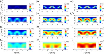
A closer look at different cross-sectional surveys at several streamwise stations are provided in figure 15. These contour plots are no longer of the narrow-band r.m.s. fluctuations approximately 75 kHz, but over different frequency ranges. The first column of plots are the disturbances between 10 and 40 kHz, the second column of plots are the disturbances between 40 and 200 kHz, and the third column of plots are the disturbances across the full bandwidth. The r.m.s. fluctuations of the mass flux across each bandwidth are normalized by the total r.m.s. of the mass flux across the full bandwidth of the measurements.
Comparison of r.m.s. contours normalized by the cross-sectional maximum full bandwidth r.m.s. across different bandwidths at select streamwise stations: (a–c)  $x = 138.4$ mm; (d–f)
 $x = 179.7$ mm;(g–i)
 $x = 192.6$ mm; (j–l)
 $x = 205.6$ mm; (a,d,g,j) 10–40 kHz; (b,e,h,k) 40–200 kHz; (c, f,i,l) full bandwidth.

At  $x = 138.4$ mm, the growth of the instabilities in the boundary layer are expected to be fairly linear. The contribution of the r.m.s. fluctuations in the lower-frequency band (figure 15a) is significantly less than the r.m.s. fluctuations in the higher-frequency band (figure 15b). The full-band r.m.s. fluctuations (figure 15c) appear to be very similar to the higher-frequency band. At a farther downstream station of
 $179.7$ mm, where the flow starts to become nonlinear, the amplitude of the instabilities in the lower-frequency band (figure 15d) starts to increase, and appears to have a significant effect on the overall r.m.s. shown in figure 15( f). As the flow approaches turbulence between
 $x = 192.6$ mm and
 $205.6$ mm, the narrow-band r.m.s. fluctuations in figure 12 no longer resemble a particular mode shape. In figure 15(g,j) the lower-frequency disturbances in the boundary layer begin to have a larger contribution to the overall r.m.s. shown in figure 15(i,l) than in the upstream
 $x$ stations. This effect is expected, but is illustrated here in mode shapes rather than in a reduced measurement of r.m.s. amplitude or power spectral density. The non-dominant lower-frequency mode shapes appear to be similar to a symmetric mode as opposed to the dominant antisymmetric mode as the flow begins to become nonlinear.
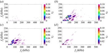
To attempt to understand possible interactions of the different modes present in the boundary layer, the autobicoherence was evaluated for the regions where the highest r.m.s. amplitude occurred in the wake of the roughness. The autobicoherence is a higher-order spectral technique that can be used to determine the coherence between waves due to wave coupling. A method of estimation of the bicoherence spectrum ( $\hat {b}^{2}$) for digital signals described by Kim & Powers (Reference Kim and Powers1979) was applied to these data and the location where the highest overall autobicoherence near the centreline is given in figure 16.
Autobicoherence for (a)  $x = 110.6$ mm, (b)
 $x = 138.4$ mm, (c)
 $x = 179.7$ mm, (d)
 $x = 192.6$ mm at the location with the highest overall autobicoherence near the centreline.

The autobicoherence shows almost no or very weak coherence at  $x = 110.6$ mm (figure 16a). Starting at
 $x = 138.4$ mm, the interaction of a 75 kHz mode with a 75 kHz mode is present at all other streamwise stations shown in figure 16, although the amplitude of this interaction is largest somewhere upstream of
 $x = 179.7$ mm. Various other interactions are shown although they are relatively weak, and this may be an indication of the source of some of the low-frequency growth. However, only a single sensor is used so these measurements show only the phase-locking of the different frequencies of instabilities.
6. Comparison of measurements to the computations
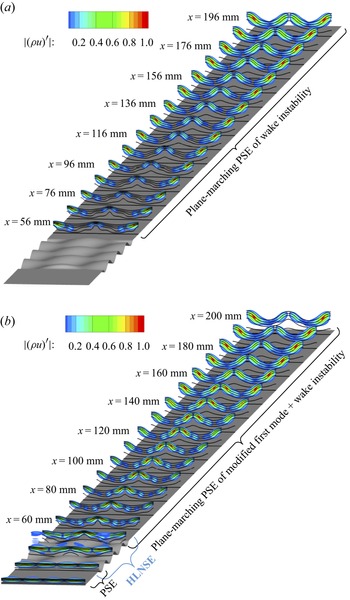
The plane-marching PSE and the combination of plane-marching PSE and HLNSE methods are used to predict the linear amplification of instabilities over the flat plate with the roughness patch. To illustrate the evolution of the instability waves, figure 17 shows the evolution of the mass-flux disturbance for the AA mode with the disturbance frequency of 80 kHz that falls within the range of most-amplified measured frequencies. Significant differences are observed between both computational procedures. The most amplified AA mode initiated downstream of the roughness wake with 80 kHz and calculated with the PSE-only method is found to peak at the off-centreline wakes adjacent to  $z/\lambda _z=\pm 0.5$ along the downstream domain (figure 17a). However, the HLNSE+PSE computations that are initiated upstream of the roughness patch showed that the most-amplified disturbance with 80 kHz corresponded to the oblique first mode with
 $\beta =2\beta _R$, which grows to an
 $N$ factor of 1.2 before the roughness insert, and the disturbance peaks switch from the on-centreline to the off-centreline wakes downstream at approximately
 $x = 160$ mm. This result agrees well with the measurements shown in figures 12 and 14, which show the different behaviour in the growth of centreline instability when compared with the growth of the off-centreline instability. The HLNSE+PSE calculation also shows how the first-mode wave morphs into the streak instability over the roughness patch. The modulation of amplitudes within the different sets of streaks is also observed in figure 18 for the AS and SA modes calculated with the HLNSE+PSE method and initiated with a first mode with
 $\beta =1.5\beta _R$ and
 $80$ kHz. The modes have a higher amplitude along the vicinity of
 $z/\lambda _z=\pm 0.5$ and
 $z/\lambda _z=0$ where the antisymmetric mode develops rather than the symmetric mode.
The AA mode shape at 80 kHz in the wake of the roughness patch, computed with (a) PSE of only the wake instabilities (PSE-only) and (b) PSE of the first mode, HLNSE of the modification of the first mode over the roughness patch, and PSE of the modified first mode and wake instability (HLNSE+PSE).

Mode shapes of the 80 kHz instabilities computed with HLNSE+PSE of modified first mode and wake instabilities for the (a) AS mode and (b) SA mode.

Measurements are not capable of detecting the initial amplitudes of disturbances at their neutral point, where disturbances begin to amplify. Thus, these initial amplitudes are frequently estimated by using the computationally predicted disturbance amplification. The comparison of the measurements and computations are first performed for the r.m.s. amplitudes of the instability in the centreline wake over a 5 kHz bandwidth centred approximately 80 kHz. Note that this is not the largest peak amplitude of the measurements, possibly because there are small differences in the surface geometry and analytic function described in the computations. The measurements were normalized by the r.m.s. amplitude at  $x = 84.7$ mm, where the measurements start to become substantially greater in amplitude than the electronic noise in the range of 70–85 kHz. The natural logarithm of this normalized amplitude is then used to estimate an initial amplitude by anchoring the value to the predicted
 $N$-factor of the dominant instability at
 $x = 84.7$ mm at the same frequency. The r.m.s. amplitude of the 80 kHz disturbance at
 $x = 84.7$ mm was approximately 0.065 % of the edge mass flux.
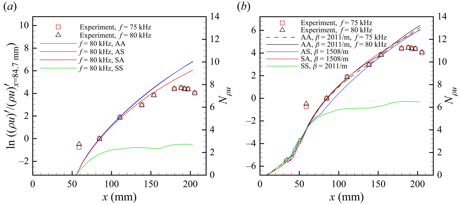
The results of this method of comparing the measurements to the two types of linear stability computations are provided in figure 19. The measurements for the 75 kHz disturbance, which was the largest-amplitude disturbance, and the 80 kHz disturbances are represented by the open square and open triangle symbols, respectively. The  $N$-factor curves are represented by solid coloured lines: black for the dominant AA mode; blue for the dominant AS mode; red for the dominant SA mode; and green for the dominant SS mode. Note that the
 $N$-factors do not account for differences in the initial amplitude of the disturbances, which are affected by the receptivity of the different modes, and that these curves follow the dominant instability in the wake of the roughness, regardless of their spatial position. These
 $N$-factor curves correspond to the vertical axis on the right-hand side of the plots. The scaling of these plots is such that the computed
 $N$ factor scaling is kept the same, and the measured r.m.s. quantities are normalized to match the computations. To compare the experimental data to the computations of linear stability, the measured r.m.s. amplitudes were anchored to the
 $N$ factor of the AA mode at
 $x = 84.7$ mm.
Comparison of measured r.m.s. amplitudes (left-hand axis) at 75 and 80 kHz with computed  $N$-factors (right-hand axis) for (a) PSE of only the wake instabilities (PSE-only), (b) PSE of the first mode, HLNSE of the first mode and PSE of the modified first mode and wake instabilities (HLNSE+PSE).

In figure 19, the computed  $N$ factors on the right-hand vertical axis range from
 $N = 0$–14 to show the
 $x$ location where
 $N = 0$ for both methods. Note that the neutral point, where
 $N = 0$, is different for each of the computational methods used. In figure 19, the scaling of the normalized r.m.s. amplitude (
 $\ln ((\rho u)'/(\rho u)'_{x=84.7 {\rm mm}}$)) on the left-hand vertical axes is set so that the range corresponds to a
 $\Delta N$ of 14. In figure 19(a), this left-hand vertical axis is offset so that measurements at
 $x = 84.7$ mm overlap with the
 $N$ factors computed with PSE at
 $f = 80$ kHz at
 $N_{\rho u} = 3.23$. This produces an estimate of the initial amplitude at the neutral point as approximately
 $2.39\times 10^{-5} \rho u_e$. In figure 19(b), the normalized r.m.s. amplitude at
 $x = 84.7$ mm for an 80 kHz disturbance is set to
 $N = 6.79$, which produces an estimate of the initial amplitude at the neutral point as approximately
 $6.80\times 10^{-7} \rho u_e$. A summary of the initial amplitudes estimated with this method are provided in table 2.
Computed  $N$ factors for the wake instability at
 $x = 84.7$ mm and estimates of the initial amplitude of the AA mode based on the measured r.m.s. amplitude of 0.065 % of
 $(\rho u_e)$ at 80 kHz.

When scaling the measured r.m.s. amplitudes in these comparisons, the measurements show excellent agreement with the computational methods at  $x = 84.7$ mm and 110.6 mm. At farther downstream stations, there is less agreement with the
 $N$-factor of the AA and AS modes in the PSE-only computations. In comparison, the HLNSE+PSE predictions of the evolution of the AA mode amplitude are in better agreement with the measured data at
 $x = 138.4$ mm and
 $x = 153.8$ mm. By
 $x = 179.7$ mm, the mode shape of the measured instability in figure 12 looks fairly nonlinear and the amplitude of the disturbance in figure 19 starts to saturate. The disturbance evolution downstream of this point is expected to be nonlinear.
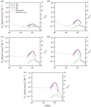
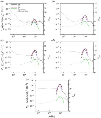
The power spectra of measurements were compared with the computations of  $N$ across a broad band of frequencies for each mode in figure 20 for the PSE-only analysis and in figure 21 for the HLNSE+PSE analysis. These comparisons are only for the assumed linear growth region of the wake and the first nonlinear station in the measurements. The power spectra of the measurements are represented by grey lines: a solid line for the spectra of the r.m.s. fluctuations near
 $z = 0.5$ mm and
 $y = 1.2$ mm; and a dashed line for the electronic noise floor. These data correspond to the left-hand vertical axis. The
 $N$-factor ‘spectra’ are represented by solid coloured lines: black for the dominant AA mode; blue for the dominant AS mode; red for the dominant SA mode; and green for the dominant SS mode. These data correspond to the right-hand vertical axis.
Comparison of power spectra to most-amplified modes computed with PSE of only the wake instabilities for (a)  $x=84.7$ mm, (b)
 $x = 110.6$ mm, (c)
 $x = 138.4$ mm, (d)
 $x = 153.8$ mm, (e)
 $x = 179.7$ mm.

Comparison of power spectra to most-amplified modes computed with HLNSE and PSE of the modified first mode and wake instabilities for (a)  $x=84.7$ mm, (b)
 $x = 110.6$ mm, (c)
 $x = 138.4$ mm, (d)
 $x = 153.8$ mm, (e)
 $x = 179.7$ mm.

The peak frequency for each of the modes computed by the PSE-only method is significantly different to the measured peak frequency. The power spectra indicate a peak frequency between 70 and 75 kHz at each of the measurement stations, but the PSE-only method (figure 20) shows a peak frequency of approximately 100 kHz for the AA and AS modes and 115 kHz for the SA mode. The SS mode has a peak frequency of approximately 150 kHz, but is not as large in  $N$-factor as the other three modes. In the HLNSE+PSE computations (figure 21), the peak frequency of the AA mode is approximately 80 or 90 kHz, while the AS and SA modes have a peak frequency at approximately 70–80 kHz. The HLNSE+PSE computations have better agreement than the PSE-only computations in describing the bandwidth of the instability peak as well. There are slight differences in the manufactured roughness and the analytic function describing the roughness (figure 5b) and this may explain some of the discrepancies between the measured peak frequency and the computed peak frequency.
In the HLNSE+PSE computations, the power spectra of the measurements have a peak centred near 75 kHz that starts to match the peak frequency bandwidth of the AS mode near  $x = 138.4$ mm. However, the r.m.s. amplitude of the 75 kHz disturbance is lower than what was predicted by the
 $N$-factor curves for the linear growth of the AA mode shown in figure 19(b). As mentioned previously, it is possible that there is some weak nonlinear interaction at this station. An inspection of the autobicoherence at this station in figure 16(b) shows that there is at least an order of magnitude higher autobicoherence near the 75 kHz and 75 kHz interaction at this streamwise location than at farther upstream stations (figure 16). While this evidence is not conclusive, it supports the likely onset of disturbance nonlinearity ahead of
 $x = 138.4$ mm.
The measurement of the AA mode in the wake means that the antisymmetric mode dominates behind each set of protuberances and dimples in the egg-crate roughness. The lack of symmetric modes in the wake of the roughness is supported by the low computed  $N$-factor given in figure 19 for the symmetric mode. The AS and SA modes include a combination of an antisymmetric mode and a symmetric mode in the wake of the roughness, and the
 $N$-factors for these two modes in figure 19 follow the growth of the antisymmetric mode in the wake because it is the larger of the two modes (figure 18). Thus, because the antisymmetric mode is the dominant mode, the AS and SA modes exhibit similar
 $N$-factors as the AA mode. Since the antisymmetric mode is the most dominant, regardless of the presence of a protuberance or dimple in the first row of the egg-crate roughness, the AA mode becomes the most-supported instability.
Figure 22 shows a side-by-side comparison of the spatial agreement of the measured modes to the 80 kHz mode computed by the HLNSE+PSE stability analysis. The HLNSE+PSE stability analysis is presented on the  $-z$ side of each figure and the measurements are presented on the
 $+z$ side of each figure. Note that there were more data in the measurements at
 $x = 110.6$ mm, so the spanwise range of the figure at this location (figure 22c) extends to
 $z = 24$ mm. As indicated in the power spectra, measurements at
 $x = 58.8$ mm are not above the electronic noise floor and no instabilities are measured in this location. At
 $x = 84.7$ mm, the regions where the instability mode are beginning to develop are large enough in amplitude to be measurable. Better agreement between the experiments and the computations are seen between
 $x = 110.6$ mm and
 $x = 153.8$ mm. However, at
 $x = 110.6$ mm, the normalization of the experimental data are affected by the amplitude of the outermost region, which is affected by the edges of the roughness insert. At
 $x = 179.7$ mm and
 $x = 188.3$ mm, the shape of the mode is larger in spatial extent than the computed mode shape, indicating some nonlinearity or saturation of the mode. At
 $x = 192.6$ mm and farther downstream, the measured mode shape at 75 kHz shows a merging of the regions with higher fluctuations while the linear stability analysis does not change. Overall, there is excellent agreement between the experiments and the computation in the region where linear growth is expected.
The r.m.s. mass-flux contours behind the egg-crate roughness for the measurement plane located at multiple streamwise stations compared with the HLNSE+PSE stability analysis:  $M = 3.5$;
 $Re = 12.6\times 10^{6}\,{\rm m}^{-1}$. Measurements from the experiment in a 5 kHz bandwidth centred at 75 kHz are given on the
 $+z$ side of the figures and the HLNSE+PSE stability analysis at 80 kHz is given on the
 $-z$ side of the figures for comparison: (a)
 $x = 58.8$ mm; (b)
 $x = 84.7$ mm; (c)
 $x = 110.6$ mm (experimental side spans from
 $z = 0$–24 mm); (d)
 $x = 138.4$ mm; (e)
 $x = 153.8$ mm; ( f)
 $x = 179.7$ mm; (g)
 $x = 188.3$ mm; (h)
 $x = 192.6$ mm; (i)
 $x = 197.0$ mm; (j)
 $x = 205.6$ mm.

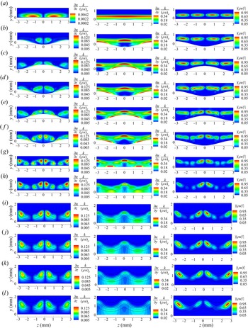
The antisymmetric mode forms over the same regions where there is a larger amplitude of the spanwise shear  $(\partial u/\partial z)$. The computed spanwise and wall-normal shear are plotted in figure 23 with the AA mode shape from the DNS. Spanwise shear is non-dimensionalized in the first column by the roughness amplitude and free stream mass flux
 $({\partial u}/{\partial z})({k}/{(\rho u)_e})$. Wall-normal shear is non-dimensionalized in the second column by the roughness amplitude and free stream mass flux
 $({\partial u}/{\partial y})({k}/{(\rho u)_e})$. The AA mode shape is non-dimensionalized by the maximum fluctuation quantity in the
 $x$ location given, as in previous figures. The black lines in each of the figures are the isolines of the mean mass flux.
The DNS of shear contours normalized by the amplitude of the egg-crate function and the free stream mass flux and comparison with mode shapes. Black lines are isolines of the mass flux. The first column is the spanwise shear, the second column is the wall-normal shear, and the last column is the computed 80 kHz AA mode shape: (a)  $x = 30.0$ mm (contour limits adjusted for spanwise shear); (b)
 $x = 35.2$ mm; (c)
 $x = 38.0$ mm; (d)
 $x = 41.3$ mm; (e)
 $x = 44.2$ mm; ( f)
 $x = 47.6$ mm; (g)
 $x = 55.0$ mm; (h)
 $x = 80.0$ mm; (i)
 $x = 120$ mm; (j)
 $x = 140$ mm; (k)
 $x = 160$ mm; (l)
 $x = 200$ mm.

Figure 23(a) depicts the first mode just upstream of the roughness and the corresponding spanwise and wall-normal shear at  $x = 30$ mm. Note that the contour levels are adjusted in the spanwise shear compared with the other streamwise locations. The adjustment to the contour levels was used to show the location of the spanwise shear more clearly. Figure 23(b) depicts the evolution of the first mode after it has passed through the first streamwise wavelength of the egg-crate roughness at
 $x = 35.2$ mm. Figure 23(c–f) (
 $x = 38$–47.2 mm) depict the evolution of the boundary layer instability as it passes over each peak and valley of the next two streamwise wavelengths in the egg-crate roughness. The AA mode develops over the roughness after the first 2.5 wavelengths (
 $x > 44.4$ mm) in the streamwise direction. The last wavelength of the roughness patch does not appear to change the mode shape significantly, indicating that more wavelengths in the streamwise direction may not greatly affect the dominant mode. Figure 23(g) shows the AA mode after the roughness patch, which begins to resemble the spanwise shear as it grows downstream.
The spanwise shear starts off stronger along the centreline as the flow passes over the egg-crate roughness pattern. As the distance from the roughness increases, the overall spatial extent of the high-shear region decreases significantly, but the spatial extent on the off-centreline wakes increases slightly at  $x = 120$ mm and becomes larger than that of the centreline region. This location is also near where the antisymmetric mode on the centreline wake becomes weaker than the antisymmetric mode in the off-centreline wake.
The relative difference between the centreline and off-centreline evolution of shear is what creates the difference in the growth of the centreline and off-centreline wakes. This effect is also noted in the measurements, where the off-centreline disturbances become stronger somewhere downstream of  $x = 153.8$ mm. The AA mode dominates for most of the flow, but once it breaks down near
 $x = 205.6$, there is a strong resemblance of the flow to the wall-normal shear.
7. Conclusions
Measurements acquired in a low-disturbance tunnel downstream of an egg-crate roughness patch show the growth of a 75 kHz AA mode at a free stream unit Reynolds number of  $12.9\times 10^{6}\,{\rm m}^{-1}$. This mode grows fairly linearly up to a station of
 $x = 179.7$ mm. Near
 $x = 179.7$ mm, the r.m.s. amplitudes of the AA mode begin to saturate and breakdown proceeds at the downstream stations. The breakdown process is characterized by a decrease in the streak amplitudes (mean flow distortion) and an increase in spectral broadening.
Computations based on a combination of plane-marching PSE ahead and along the wake of the roughness patch and the three-dimensional HLNSE over the roughness patch indicate good agreement with the disturbance amplification measured during the linear phase. The stability analysis also shows that the antisymmetric mode has higher growth in the wake of all of the surface features of the egg-crate roughness. This conclusion is further supported by the appearance of only the AA mode in the measurements.
Computations using only PSE are similar to what is typically performed for linear stability analysis for the wake of a roughness element. This is not surprising, considering the required computational power is approximately two orders of magnitude less for the PSE-only computations compared with the HLNSE+PSE computations. In cases where the modulation of the mean flow by the roughness is not significant, or where rapid results are desired (i.e. during a design process), the PSE-only computations may be sufficient to determine transition due to roughness.
In the case of the egg-crate roughness, previous DNS show a significant modulation of disturbances upstream of this sinusoidal roughness patch, which have now been confirmed by both the HLNSE+PSE computations as well as the experimental measurements. This joint experimental and computational study is the first to use a combination of HLNSE and PSE for a three-dimensional geometry to predict the growth of instabilities in the wake of a distributed roughness patch and complementary measurements in a wind tunnel experiment. The agreement of the computations and complementary measurements shows the importance of considering the modification of instability modes by surface roughness and the effect on the development of downstream disturbances.
Acknowledgements
This work was performed under the Revolutionary Computational Aerosciences discipline under the Transformational Tools and Technologies Project of the NASA Transformative Aeronautics Concepts Program.
Declaration of interests
The authors report no conflict of interest.