Introduction
There are two opposing approaches in visual perception, bottom-up and top-down, each with a long history. But the recently prevailing view is that there are two simultaneous streams of information which interact. This interaction is actualized at the output of preattentive processing. But this leaves an unresolved issue: what is this output?
In the 1980s, one of the popular theories assumed that the result of the preattentive processing is a set of local features. Visual attention is a binding mechanism for these features (Treisman & Gelade, Reference Treisman and Gelade1980). Later, other models with the active role of the selective attention were proposed (Di Lollo et al., Reference Di Lollo, Kawahara, Zuvic and Visser2001; Logan & Gordon, Reference Logan and Gordon2001; Wolfe et al., Reference Wolfe, Horowitz, Kenner, Hyle and Vasan2004; Cohen et al., Reference Cohen, Schnitzer, Gersch, Singh and Kowler2007). The similarity of these models is that the top-down impact is directed to local operators (striate neurons) which are the output of preattentive processing.
Later, a new approach to the binding problem was developed. This proposed two stages in preattentive processing (Babenko, Reference Babenko and Kogan1989; Chubb & Sperling, Reference Chubb and Sperling1989; Sutter et al., Reference Sutter, Beck and Graham1989; Victor & Conte, Reference Victor and Conte1989). The first one occurs as simple striate neurons reacting to luminance gradients (the first-order mechanisms). The second stage is represented by the elements connecting the outputs of adjacent first stage filters (the second-order mechanisms). Spatial pooling of local information is realized by a rigid algorithm, while the selective attention deals with the prepared pools (Kahneman & Henik, Reference Kahneman, Henik, Kubovi and Pomerantz1981; Treisman, Reference Treisman, Boff and Kaufman1986; Duncan & Humphreys, Reference Duncan and Humphreys1989).
Generally, the spatial binding which occurs at the initial stages of visual processing may be reduced to two main operations: contour integration and pooling of the surface elements. It is assumed that the first operation can be started at the level of striate neurons by means of lateral communications (Ts'o et al., Reference Ts’o, Gilbert and Wiesel1986; Gilbert & Wiesel, Reference Gilbert and Wiesel1989; Hirsch & Gilbert, Reference Hirsch and Gilbert1991; Das & Gilbert, Reference Das and Gilbert1999) or feedbacks (De Weerd et al. Reference De Weerd, Sprague, Raiguel, Vandenbussche and Orban1993, Reference De Weerd, Sprague, Vandenbussche and Orban1994, Reference De Weerd, Desimone and Underleider1996; Merigan Reference Merigan1996), and is based on the influences from the outside of the receptive fields (Kapadia et al., Reference Kapadia, Ito, Gilbert and Westheimer1995; Polat et al., Reference Polat, Mizobe, Pettet, Kasamatsu and Norcia1998; Sugita, Reference Sugita1999; Albright & Stoner, Reference Albright and Stoner2002). The other operation integrates local information in a two-dimensional space (Babenko, Reference Babenko1990; Chubb & Landy, Reference Chubb, Landy, Landy and Movshon1991; Graham et al., Reference Graham, Beck and Sutter1992; Dakin & Mareschal, Reference Dakin and Mareschal2000). It is realized by the so-called second-order filters which combine the outputs of the adjacent first-order filters (simple striate neurons) within a limited area. This integrating mechanism is usually described by the “filter-rectify-filter” model. It is believed that these are the second-order filters that provide preattentive texture segregation and perception of the second-order motion (e.g., a shift of a contrast edge in a stationary carrier).
The spatial organization of these mechanisms has been actively studied in recent years (Landy & Oruç, Reference Landy and Oruc2002; Prins et al., Reference Prins, Nottingham and Mussap2003; Ellemberg et al., Reference Ellemberg, Allen and Hess2006; Babenko et al., Reference Babenko, Ermakov and Bozhinskaya2010, Reference Babenko, Yavna, Soloviev and Miftakhova2011; Sun & Schofield, Reference Sun and Schofield2011; Reynaud & Hess, Reference Reynaud and Hess2012; Westrick et al., Reference Westrick, Henry and Landy2013; Baker & Meese, Reference Baker and Meese2014). But the model introduced 20 years ago still remains the established account (for review, see Wilson, Reference Wilson1999). One of the main properties of this model is its nonspecificity with respect to the modulated parameter of the texture. In other words, the second-order mechanisms have to show an identical reaction to any texture border, irrespective of whether it was formed due to a change in contrast, orientation, or spatial frequency of its elements (Kingdom et al., Reference Kingdom, Prins and Hayes2003).
On the one hand, this nonspecificity is appropriate in forming a general, universal “salience” map that guides the segmentation process of the visual scene. On the other hand, information concerning the modulation dimension is also important since the modulations of contrast, orientation, and spatial frequency (CM, OM, and FM, respectively) provide information on the shape, orientation, and surface position.
The specificity of the second-order mechanisms can be investigated psychophysically by means of an interaction paradigm. Kingdom et al. (Reference Kingdom, Prins and Hayes2003) failed to find interactions between CM, OM, and FM. However, they concluded that there is a single multichannel mechanism. The absence of interactions was accounted for the process of contrast normalization. In contrast, Schofield and Yates (Reference Schofield and Yates2005) revealed weak interaction between CM and OM, but proposed a model consisting of specific mechanisms: CM was detected by broad-band channels, while OM was detected by opponent channels. Afterward new psychophysical data suggested dissimilarity of the second-order visual mechanisms but did not directly answer the question about their specificity (Olzak & Kramer, Reference Olzak and Kramer2007; Schofield et al., Reference Schofield, Ledgeway and Hutchinson2007; Babenko & Yavna, Reference Babenko and Yavna2008). Thus, we have to admit that the problem of the second-order visual filters specificity still remains unresolved by the psychophysical approach.
The solution of the problem could be facilitated by the data obtained through objective investigation methods. If the second-order mechanisms are nonspecific, then they should have a common location within the cortex and give identical response to different modulations. But if they are specific, then they might have different locations and their own response peculiarities.
Some hopes to solve the problem were associated with the investigation of neurons in different visual areas. However, ambiguous answers were also obtained. The peculiarities, which were inherent in the second-order visual mechanisms, were revealed in the neurons at: V1 (Grosof et al., Reference Grosof, Shapley and Hawken1993; Chaudhuri & Albright, Reference Chaudhuri and Albright1997), V2 (El-Shamayleh & Movshon, Reference El-Shamayleh and Movshon2011), V3 (Gegenfurtner et al., Reference Gegenfurtner, Kiper and Levitt1997), V4 (Ghose & Ts'o, Reference Ghose and Ts’o1997), MT (Olavarria et al., Reference Olavarria, De Yoe, Knierim, Fox and Van Essen1992; Lui et al., Reference Lui, Bourne and Rosa2007), IT (Sáry et al., Reference Sáry, Vogels, Kovacs and Orban1995) and even at LGN (Pengjing et al., Reference Pengjing, Xiang and Yifeng2007; Rosenberg et al., Reference Rosenberg, Husson and Issa2010) and retina (Demb et al., Reference Demb, Zaghloul and Sterling2001).
Progress toward solving this problem can be achieved by the use of visual evoked potentials (VEPs). In such experiments, the functioning of the second-order visual mechanisms may be represented by a wave which is calculated by subtracting VEP to a uniform texture from VEP to a modulated one (d-wave). Different stimuli and visual tasks have been used in such investigations (e.g., Lamme et al., Reference Lamme, Van Dijk and Spekreijse1994; Caputo & Casco, Reference Caputo and Casco1999; Calvert et al., Reference Calvert, Manahilov, Simpson and Parker2005). The general result of these studies was that any texture gradient causes an increase in negativity of VEP with the latency of about 200 ms. But these results do not answer the question posed above. One has to compare the d-waves for different gradient dimensions obtained under identical conditions, i.e., within the same experiment. Such studies are rare. But even in them (Bach & Meigen, Reference Bach and Meigen1999; Fahle et al., Reference Fahle, Quenzer, Braun and Spang2003) researchers primarily used those spatial gradients that can be detected as early as the first-order mechanisms (gradients in luminance, color, or stereoscopic depth). However, Bach et al. (Reference Bach, Schmitt, Quenzer, Meigen and Fahle2000) used gradients that involved the second-order mechanisms. The authors concluded that the mechanisms for processing different texture gradients partly overlap. Unfortunately, there was only one electrode (Oz) in this study.
Ten years later, Straube et al. (Reference Straube, Grimsen and Fahle2010) used gradients of orientation and spatial frequency again; now there were 25 electrodes. It was found that the d-waves for different gradients are of similar amplitude if subjective saliencies of these gradients are equalized. Unfortunately, this fact tells us nothing about the organization of the second-order visual mechanisms. Such a result is possible for both a single processing mechanism and several specific mechanisms. Furthermore, one should not just compare the response magnitudes, but show possible discrepancies in temporal and spatial domains. The goal of our study was to determine if the evoked activity was specific to the modulated texture parameter (modulation dimension).
To answer this question, it was necessary to create stimuli that were similar in all parameters except the modulation dimension (contrast, orientation, or spatial frequency), so that the stimuli would produce an equalizing total effect on the first-order mechanisms while creating a condition for selective activation of the second-order mechanisms. Guided by these considerations, we created an initial (NM) texture consisting of vertically oriented Gabor micropatterns. The Gabor patches selectively activate striate neurons in a corresponding location, orientation, and spatial frequency of the luminance gradient.
If the orientation of the texture elements is modulated, the activity shifts from the neurons tuned to the vertical, to the neurons tuned to the tilt. Wherein, the total first-order filters activity does not substantially change, neither does its contribution to VEP generation.
A similar picture is observed for FM. The number of the activated striate neurons tuned to the initial frequency decreases, at the same time those neurons tuned to lower and higher spatial frequencies are activated.
However, CM inevitably leads to the formation of side-bands, i.e., side peaks in the frequency spectrum. This can actually cause the activation of additional striate neurons. We compared the power spectra of our NM and CM textures. It appeared that the total spectral power of the CM texture was only 5% higher, and such a small difference can be ignored.
Here, we do not intend to discuss the side-band problem in detail because it is more relevant for the task of modulation detection than modulation discrimination. Introduction of additional frequency (and perhaps orientation) components may be a key factor where CM is detected. In such a case, a decision is possible at the level of the first-order visual mechanisms. But we used a discrimination task for those modulations which were superthreshold. Side-bands are not useful in a discrimination task. It is much easier for the observer to make a decision focusing on the envelope than on the spectral characteristics of the texture. We emphasize once again that the appearance of side-bands does not significantly alter the total activity of the first-order filters.
The side band problem may not be the only factor that affects the validity of our stimuli as drivers for the second-order visual mechanisms. The observer can potentially solve the offered experimental task focusing on the carrier, not on the envelope. It is sufficient to attend the local part of the texture which, for example, corresponds to the modulation peak, in order to assess the modulation dimension by the change in contrast, orientation, or size of a single texture element. To reduce this possibility, we used a random shift of the modulation phase. But this manipulation does not exclude the fact that the experimental task can sometimes be solved at the local level. Nevertheless, this fact cannot distort the experimental results. Since the second-order visual mechanisms are preattentive (Chubb & Sperling, Reference Chubb and Sperling1989; Sutter et al., Reference Sutter, Beck and Graham1989; Kingdom & Keeble, Reference Kingdom and Keeble1999; Ellemberg et al., Reference Ellemberg, Allen and Hess2006 and others), their response is automatic regardless of the intentions of the subject.
Thus, we have every reason to believe that if we find changes in VEPs as a result of texture modulation, it will mean a change in activity at the second-order filters level, not at the first-order filters level.
Planning the experiment, we assumed that if the d-wave parameters for different modulations appeared to be different, it would testify to the specificity of the second-order visual mechanisms.
Materials and methods
Subjects
A total of 48 students (22 men and 26 women) between the ages of 18 and 34 (mean age 24.4, standard deviation 3.7) took part in this investigation. All the participants had normal or corrected to normal vision and reported no history of neurological or psychiatric disorders. Research participants reported that they had not taken any medical drugs immediately before or during the study tests. All the research participants were informed about the purpose and procedures of the experiment; they all signed a consent form that outlined the risks and benefits of participating in the study and indicated that they believed in the safety of the investigation. The study was conducted in accordance with the ethical standards consistent with The Code of Ethics of the World Medical Association (Declaration of Helsinki) and approved by the local ethics committee.
Apparatus
All stimuli were displayed on a 17" LG Flatron 775FT (LG Corporation, Seoul, Korea) monitor hosted by a PC (i386-compatible) using Linux Ubuntu OS with an Intel 915G based graphical subsystem. The screen resolution was 1024 × 768 pixels with a frame rate of 85 Hz. The monitor luminance was calibrated by means of a digital photometer (manufactured by “TKA”, St. Peterburg, Russia) using 256 gray levels. A luminance and contrast were adjusted so as to maximize the total range of luminance alongside with minimizing the luminance change step. To invert the gamma nonlinearity, we used the exponential associate function.
EEGs were recorded with a Neurobotics Neurovizor-BMM40 digital amplifier connected to a PC with an OS Windows XP platform.
Stimuli
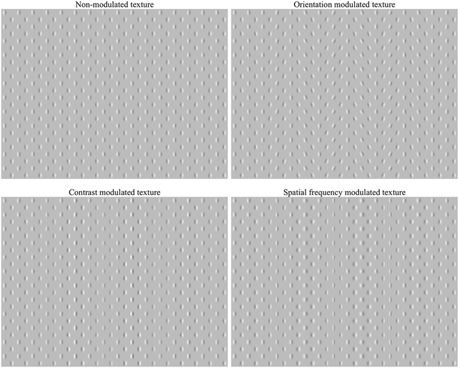
All the stimuli were textures composed of Checkerboard matrix of Gabor patches. The size of the conventional checker squares that had patches in their center was 0.44 × 0.44 angle deg. In all, a total of four textures were used: NM, CM, OM, and spatial FM (see Fig. 1). The spatial frequency of the carrier was 3.5 cpd in NM texture, all patches had vertical orientation, and their contrast was 0.5. The modulation function was set by a horizontal sine curve of 0.3 cpd frequency. A random shift of the modulation phase was used. The modulation amplitude (maximum parameter difference in the display) was 3 dB for contrast, 20 deg for orientation, and 1 octave for spatial frequency. The textures filled the screen which had a size of 14 × 10.5 angle deg. The mean luminance of all stimuli was the same as that of the uniform background, at 30 cd/m2. Each stimulus was presented for a total duration of 500 ms.
Experimental stimuli.

Procedure
Training
All the study participants were trained by all the stimuli used in the experiment. Initially their exposure was long (2 s), but it was gradually decreased to the experimental duration (0.5 s). The training was stopped when the level of the correct responses exceeded 80%.
Experimental setup
The observers sat at a distance of 130 cm from the monitor screen and were requested to fix their gaze at the center of the screen. Each of the four textures was presented 150 times at a random sequence. The intervals between the stimuli were filled by blanks (gray screen 30 cd/m2). The observers were to identify the texture by selecting one of the four keys on the computer keyboard. These keys were located in the right hemifield. All the observers only used their dominant hand to respond (all the subjects were right-handers). The response time was not limited. This led the observer to make a rest pause if necessary. All the participants were instructed to blink only when they gave answers in order to avoid artifacts in VEPs. The interval between the answer and the presentation of the next stimulus varied randomly between 1 and 3 s. In case the observers identified the experimental stimulus incorrectly, they could hear a brief audio signal. The experiment was finished if the quota of incorrect decisions exceeded 30%, and then the observer was retrained.
The EEG recordings were made in a monopolar mode with 20 sintered Ag/AgCl ring scalp electrodes and Brain-Cap, labeled according to the 10–20 international system (Fp1, Fp2, F7, F3, Fz, F4, F8, C3, Cz, C4, T3, T5, T4, T6, P3, Pz, P4, O1, Oz, O2). A “linked ears” reference scheme was used. The ground electrode was positioned in front of Fz. The electrode impedance was kept below 10 kΩ. Simultaneously, an oculogram was recorded. The trigger marks contained information on the stimulus type and the onset moment. The EEG recording was made within a frequency band of 0.5 to 40 Hz. The EEG signal digitalization frequency was 1 kHz.
Data analysis
EEG epochs of −100 ms to +500 ms duration against the stimulus onset were used for further averaging. EEG records with eye blink artifacts, eye movements, extensive muscular activity, or other noise within this window were excluded from further analysis. The remaining epochs were averaged separately for each stimulus type (not less than 90 epochs within each pool). The mean signal of 100 ms time window prior to the stimulus onset served as a baseline correction. The result per each observer was four VEPs for each electrode site.
Then VEP to NM texture was subtracted from VEP to each of the modulated textures. This way three different waves (d-waves) (OM-NM, FM-NM, CM-NM) were obtained for each electrode site.
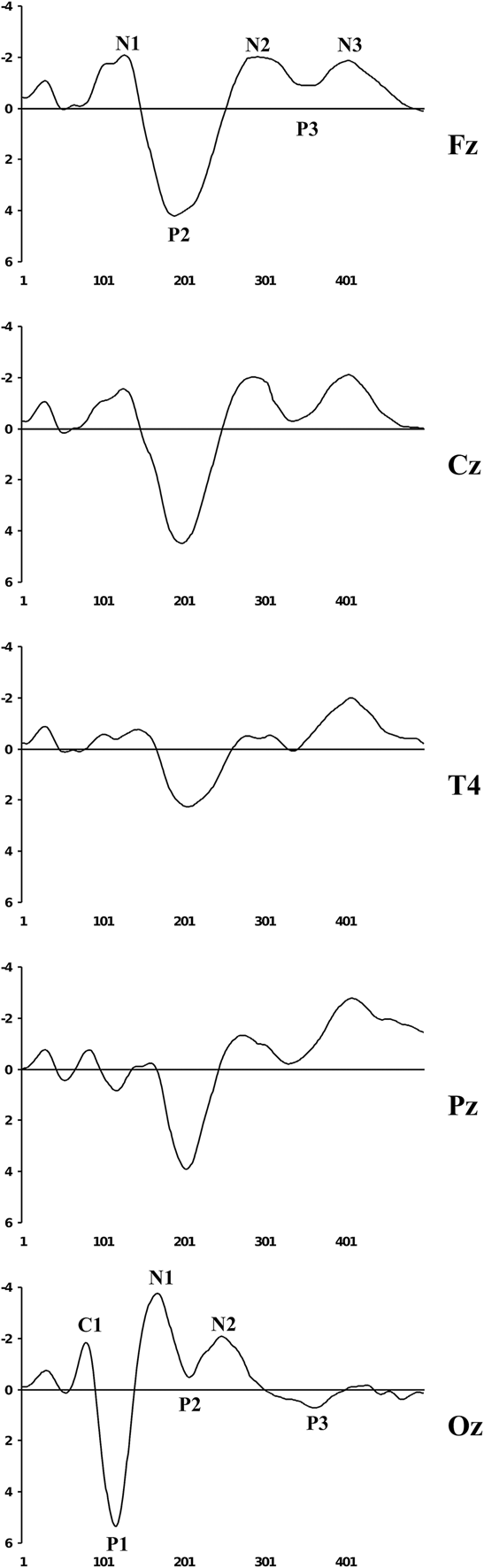
VEPs and d-waves were then separately grand-averaged. Fig. 2 shows the grand-averaged VEPs for NM texture for different cortex areas with an indication of the basic components according to the generally accepted classification (Luck, Reference Luck2005). The basic analyses were conducted by comparing the grand-averaged d-waves with T-tests, their topographic mapping, with the use of sLORETA. This method (sLORETA) was specifically designed for a limited number of electrodes (19 or more) (Pascual-Marqui, Reference Pascual-Marqui2002).
Grand-averaged VEPs at different electrode sites by component designation. Zero denotes stimulus onset. X axis – stimulus time (ms), Y-axis – potential amplitude (μV).
Results
Orientation modulation
VEP component analysis
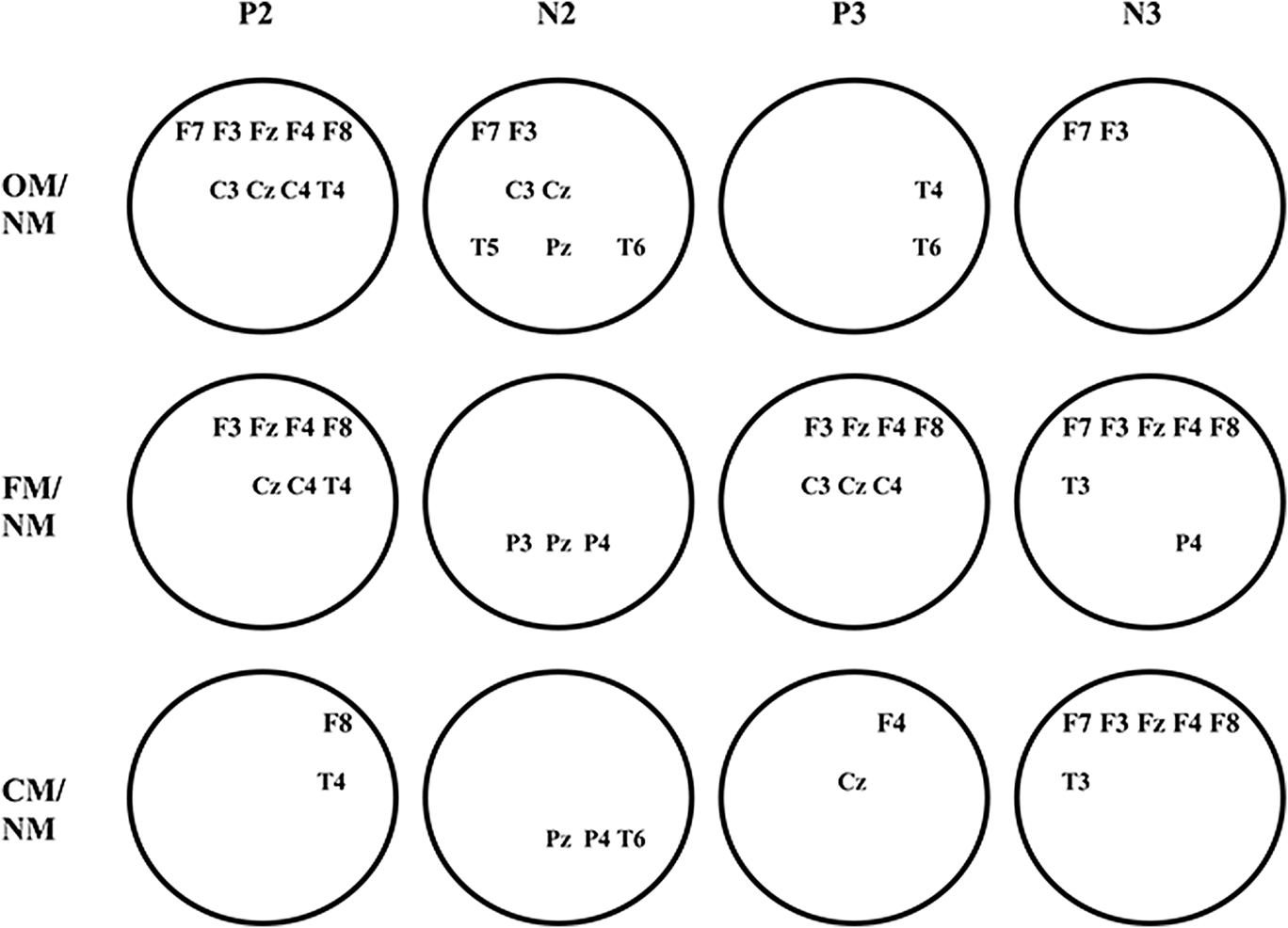
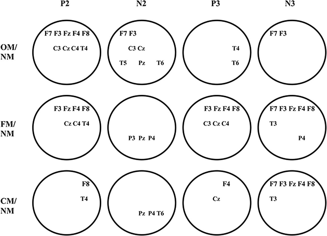
A number of differences are revealed if one compares VEP to OM texture with VEP to NM texture. The texture modulation does not affect the early components of VEP (C1, P1, and N1), but leads to changes in the subsequent waves. Specifically, the P2 amplitude decreases, but N2 and P3 increase at all occipital electrode sites (T-test, P < 0.01). Other cortex areas showed significant amplitude increases in VEP components having a latency of more than 200 ms. However, the longer latency of VEP component, the smaller the number of the electrodes where such changes are statistically significant (Fig. 3, top row). These changes became more and more lateralized as the latency increased.
Layout of leads for statistically significantly different VEPs (T-test, P < 0.01). Occipital electrodes are not shown. On the left are comparison stimuli. Above shown are those VEP components whose amplitudes were compared.
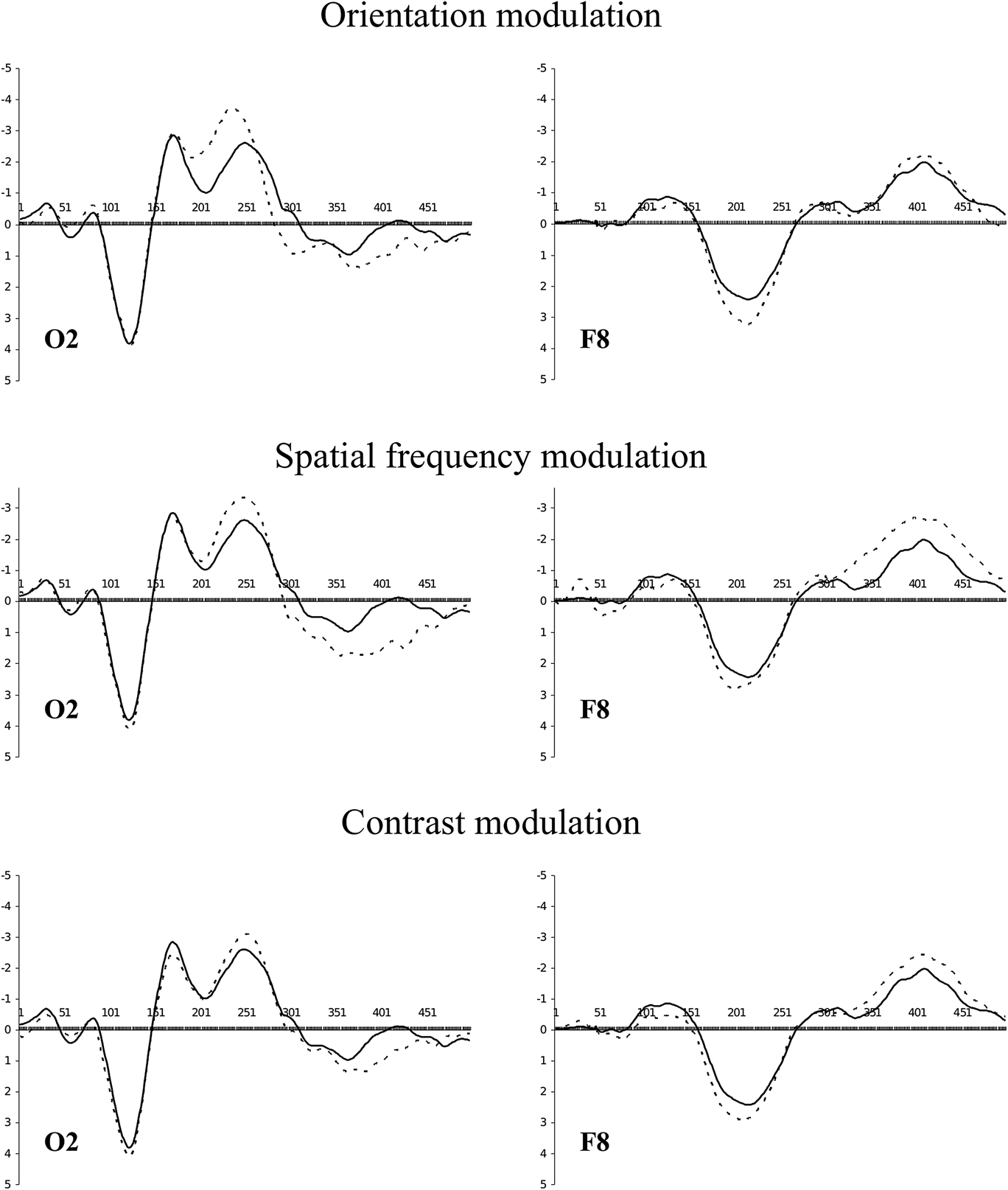
The revealed P2 and N2 changes in occipital VEPs resulted from an increase in negativity, while the P3 changes were due to an increase in positivity (Fig. 4, top line, left). Within more rostral areas, a reverse process occurred: first, on the P2 wave, positivity increases, and then, on the N3 wave, negativity rises (Fig. 4, top line, right). Thus, in the hind brain, negativity changed to positivity, while in other areas this order was reversed.
Grand-averaged VEPs for NM (solid line) and modulated (dotted line) textures.
d-wave component analysis
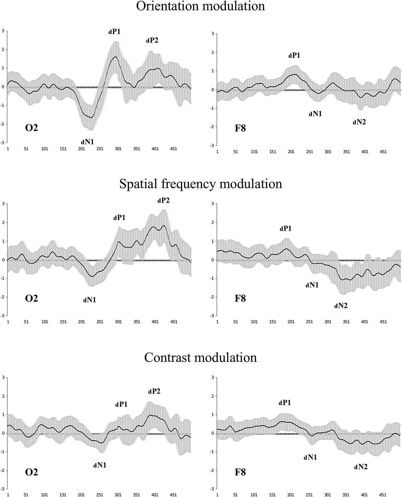
After the subtraction of VEPs and averaging of the obtained waveforms at each electrode site over all the observers, we obtained the results that are partly shown in Fig. 5 (top row). The d-waves consisted of three components at the occipital electrode sites. The first component reflected the growth of negativity, while the second and third components yielded increases in positivity. Specifically, the first d-wave component resulted in a growth of negativity during the P2 and the leading edge of N2. The second d-wave component was associated with a rise in positivity at the P3 leading edge, while the third component reflected an increase in positivity at the P3 trailing edge. The frontal d-waves also contained three components, which were however formed in the opposite phase to the occipital d-waves and characterized by a significantly lesser amplitude. The first component reflected the growth of positivity during the P2, while the second and third components, though not evident at every electrode site, reflected the growth of negativity during the N2 and N3, respectively.
Grand-averaged d-waves (grand mean across 48 observers). The shaded area around the wave depicts the confidence interval (P < 0.01). Amplitude deviations from zero are not stochastic where the confidence interval does not cross the X axis. There are component designations for the d-waves. In order not to confuse them with the VEP components, the d-wave components are provided with the index “d”.
d-wave topography analysis
Tracing the time dynamics of the d-wave topography shows that the analyzed potentials in the frontal-central areas somewhat outran those in the occipital area.
The first d-wave component is shown as positivity in the frontal-central areas and as negativity in the hind brain (Fig. 6, top line). The picture clearly indicates that the frontal positivity is formed by 180–200 ms, and outran the occipital negativity by about 20 ms. The first component reaches its maximum by 200–220 ms. A shift toward the right hemisphere is also observed.
Topography of the first d-wave component for top of the head. Scalp topographic voltage maps for latency range 160–280 ms in 20 ms intervals; voltage scale shown on the right in vertical bars. Voltage scale range from −2 to 2 μV.
The second d-wave component is also accompanied by the formation of two poles (Fig. 7, top line). This time negativity is formed in the frontal areas of the left hemisphere, while there is positivity in the occipital areas of the right hemisphere. This process reaches its peak at about the 290–300th ms.
Second d-wave component topography. Scalp topographic voltage maps for latency range 280–340 ms in 10 ms intervals; voltage scale shown on the right in vertical bars. Voltage scale range from −2 to 2 μV.
During the third d-wave component, the pole positions remain unchanged (Fig. 8, top line), but now a left-side asymmetry is characteristic for frontal negativity along with occipital positivity. The peak for this activity occurs at approximately 400–420 ms.
Third d-wave component topography. Scalp topographic voltage maps for latency ranges 340–460 ms in 20 ms intervals; voltage scale shown on the right in vertical bars. Voltage scale range from −2 to 2 μV.
However, the potential topography on the head surface is a poor index of the real dynamics of the electrical processes occurring in the cerebral cortex. In fact, advancing formation of positivity in the frontal areas and delayed negativity in the posterior areas may, for example, indicate the existence of two activity regions, one formed before the other. But these phenomena may be conditioned by changes in the orientation of the dipole source that has no relation to the above-mentioned areas. In this regard, additional analyses of the results were conducted.
d-wave sLORETA analysis
To analyze the obtained d-waves, we used the standardized low-resolution electromagnetic tomography method (Pascual-Marqui, Reference Pascual-Marqui2002) named sLORETA. This method enables to localize in the cortex of equivalent current 3D density distribution (registered activity sources) maximums. d-waves were used as input data.
In spite of the fact that every d-wave component was accompanied by the formation of two poles on the topographical map (frontal and occipital), in all these cases sLORETA showed the occipital activity focus only. Thus, the peak of activity during the first d-wave component fell on the 223rd ms and was localized in area 19 of the right hemisphere (Fig. 9, top line, the first one on the left). However, the occipital cortex of the left hemisphere is also active, though to a lesser extent.
The images of neural activity computed with sLORETA for back views of the head. Peaks of activity associated with the formation of the d-wave components are shown. Captions under the figures refer to: peak latency/focus activity magnitude. Color scale represents sLORETA units.
Activity during the second d-wave component grows up to 296 ms, its focus staying in area 19 of the right hemisphere (Fig. 9, top line, the second one on the left). However, the source density reduces more than twice against the first component, while the activity in the left hemisphere fades away almost completely.
The third d-wave component appeared to include two consecutive peaks of activity (Fig. 9, top line, two right ones). The first peak is formed at 391 ms with as focus on area 19. The second peak of activity falls at 442nd ms; in magnitude and localization, it replicates the previous peak. It should be noted that during the entire third component, activity is localized in the left hemisphere.
Thus, the formation of the d-wave produced by OM involves area 19. It is also noteworthy that the first two peaks of activity are located in the right hemisphere, while those that follow are found in the left hemisphere.
Spatial frequency modulation
FM leads to VEP changes similar to those found in OM stimuli. However, a more detailed analysis revealed important differences.
VEP component analysis
FM does not affect P2 but significantly increases N2 and P3 amplitudes at all occipital electrode sites (T-test, P < 0.01). In other areas, especially in the frontal-central ones, there was an increase of P2, N2, N3, and a decrease of P3 (Fig. 4, middle line). At the same time, the topography of those electrode sites where the noted differences are statistically significant essentially changes against OM (Fig. 3, middle line). This is especially a characteristic of the late response components.
The revealed differences in VEPs for FM were similar to those found for OM: growth of negativity changes to growth of positivity in the occipital electrodes, while it was the other way around in the anterior areas (Fig. 4, middle line). However, VEP changes caused by FM, as compared to OM, were less expressed up to the 300th ms and more expressed after that.
d-wave component analysis
The results of subtraction of VEPs to NM texture from VEPs to FM texture are shown in Fig. 5, middle line. The waveforms for FM were similar to those during OM. The difference was that the first two components of the d-wave for FM were of a lesser amplitude, particularly for the frontal and central electrodes. But the third component had larger amplitude than for OM.
d-wave topographic analysis
If one traces the time dynamics of topography of the first d-wave component for FM (Fig. 6, middle line), it becomes obvious that the anterior advance is more pronounced than for OM. This is mainly due to a later formation of posterior negativity for FM. Frontal positivity is formed by 180 ms (the same as for OM), while occipital negativity is only formed by 220 ms (that is roughly 20 ms later than for OM) when frontal positivity is already declining.
As in the case of OM, positivity and negativity change places during the second d-wave component evoked by FM (Fig. 7, middle line), but it happens 10–20 ms later.
There is a pause of 20–30 ms between the second and third d-wave components for OM, whereas this pause is absent for FM. First, polarity growth was due to the increase of frontal negativity, and after that to the increase of occipital positivity. Like in the case of OM, polarity reaches its maximum by 400–420 ms but becomes more expressed as its formation starts 30–50 ms earlier.
d-wave sLORETA analysis
Despite the fact that the time shift between the anterior positivity and posterior negativity increases for FM in comparison with OM, sLORETA still shows only one focus of activity for the first d-wave component (as for the next components). Activity reaches the first maximum at 210 ms, which is by 13 ms faster than for OM (Fig. 9, middle line, the first on the left). Activity covers both hemispheres and its focus is also localized on the right. But now it is area 18. Different also is the density of sources: it is significantly lower (about 5 times) for FM.
In contrast, the second activity peak was formed 17 ms later (313 ms) than for OM, not in the right, but rather in the left hemisphere (Fig. 9, middle line, the second on the left), its focus located in area 17.
The third d-wave component for FM also had two activity peaks as for OM (Fig. 9, middle line, two right ones). The first activity maximum climbed at 397 ms and was localized in area 19 of the right hemisphere. After 24 ms, the second activity peak was formed in the same area. In contrast to OM, both activity peaks were formed in the right hemisphere.
Thus, activity peaks for the two compared modulations (OM and FM) did not coincide in location, formation time, or in magnitude. Peculiarities were observed in hemispheric activity dynamics. It is identical for the first activity peak only. Later, the different hemispheres are activated for FM and OM.
Contrast modulation
VEP component analysis
The spatial contrast modulation of texture elements produced similar changes in VEPs compared to the responses to NM texture. Amplitudes of N2 and P3 grow at the posterior electrode sites, but statistically significant changes (T-test, P < 0.01) were only detected in the right hemisphere (Fig. 3, bottom line). In other areas, changes occurred in each VEP component having latency over 200 ms. However, the spatial distribution of those electrodes where the changes are statistically significant differs from what we noted for OM and FM. First, the number of such electrodes was dramatically reduced (except N3). Second, P2, N2, and P3 showed a distinct right-sided asymmetry.
Similar to previous observations, VEP changes caused by CM are the result of the fact that growth in negativity is replaced by growth in positivity at the occipital electrode sites near 300 ms whereas there is a reverse process in the other electrodes (Fig. 4, bottom line).
d-wave component analysis
After subtraction of VEPs to NM texture from VEPs to CM texture, we calculated averaged d-waves, partially shown in Fig. 5, bottom line. Once again, the d-waves have three components, but are expressed to a lesser degree than for other used modulation dimensions.
d-wave topography analysis
What concerns d-waves topography time dynamics, the result has its own characteristics. During the first d-wave component, frontal positivity starts forming at approximately the same time as with other modulations, that is somewhere close to the 180th ms. But activity was clearly lateralized to the right hemisphere. Occipital negativity formation was delayed by 60–80 ms in comparison with frontal positivity (Fig. 6, bottom line).
The second d-wave component was nearly absent (see Fig. 5, bottom line). The topographical maps for this time period produced only insignificant changes: near 300–310 ms some occipital positivity was formed and shifted to the left hemisphere (Fig. 6, bottom line). At the same time, frontal negativity was only weakly expressed.
But the anterior negativity starts to grow from 320 ms and it is the origin of the third d-wave component. Later (after about 30 ms) the anterior negativity is added by the posterior positivity. Both poles are formed up to 400–420 ms.
d-wave sLORETA analysis
For CM, similar to the results for other modulations, both hemispheres were involved during the initial phase of activity which is the base for the first d-wave component. Besides, the coordinates for the first activity peak were located in area 18 of the right hemisphere and coincided with the coordinates of the first peak for FM. They also have similar source density values. However, its latency for CM is longer (228 ms against 210 ms) (Fig. 9, bottom line, the first on the left).
The same as for FM, the second activity wave shifted to the left hemisphere, but was lesser in magnitude and formed 13 ms earlier with a more rostral localization (in area 18) (Fig. 9, bottom line, second on the left).
The third d-wave component, as found in other modulations, comprised two activity peaks (Fig. 9, middle line, two right ones). The first peak formed at 391 ms but it occurred in the right hemisphere (area 18). Then, after 34 ms, the second activity peak is formed in area 19 of the same hemisphere. Thus, interhemispheric dynamics for CM coincided with the activity dynamics for FM.
Discussion
The results demonstrate that activity changes caused by different texture parameter modulations had both common and specific features. Let us start with a discussion of the common features.
First, VEP changes caused by texture modulations did not affect early response components (C1, P1, N1). The d-waves had a latency of about 200 ms. These results fully agree with other research on negativity growth at occipital electrode sites to the static second-order stimuli: textures modulated in orientation (Lamme et. al., Reference Lamme, Van Dijk and Spekreijse1992; Bach & Meigen, Reference Bach and Meigen1999), contrast (Calvert et al., Reference Calvert, Manahilov, Simpson and Parker2005), and spatial frequency (Bach et. al., Reference Bach, Schmitt, Quenzer, Meigen and Fahle2000).
Second, the negativity growth changes to the positivity one between 200 and 300 ms. This coincides with the data from Straube et al. (Reference Straube, Grimsen and Fahle2010).
Third, we found that when negativity changed to positivity in the occipital area there was an inverse dynamics in the anterior locations. In that, the d-wave first arises at the fronto-central electrode sites and only after some time it appears in the occipital ones.
Thus, the overall view of the d-wave is identical for all the modulation dimensions used in this study. This means that the general sequence of the brain processes was similar in the perception of different texture modulations. What processes are meant here?
The processes related to texture perception theoretically look as follows (for review, see Graham, Reference Graham2011). Initially, the first-order visual mechanisms are activated. These mechanisms are sensitive to luminance gradients and carry out linear filtering in local image areas; i.e., they process separate texture elements in parallel. This operation is associated with the earliest VEP components (Luck, Reference Luck2005). Then, the rectified responses of the first-order filters arrive at the second-order filters inputs. These reactions are transferred to the next, “third” processing level as well. If the texture is not modulated, then the second-order filters will not be activated, and the third level receives signals from the first-order filters only. Should the texture be modulated, then signals from the second-order filters are added to them.
We propose that the first d-wave component (frontal dP1 and occipital dN1 in Fig. 5) coinciding with P2 reflects the second-order filters functioning. The second component of the d-wave (frontal dN1 and occipital dP1) begins right after the first one and falls on P3 which is associated with the processes of classification and decision-making (Picton, Reference Picton1992; Polich & Kok, Reference Polich and Kok1995). Seemingly, the reactions of the first and second-order filters are combined at this stage. The third component of the d-wave (frontal dN2 and occipital dP2) is formed with a latency period of about 450 ms and precedes the motor response of the subject. But it is not a motor response command because the latency of the action has always been much longer. It is rather a representation of a decision which key to press.
We now ask: how far may this sequence of events be true? Why is the d-wave latency so large? Why does the first negativity occur on VEP component traditionally associated with the attention processes? Should we not expect earlier changes of VEPs, which would be more in line with the bottom-up model of preattentive vision? Sure enough, according to psychophysical data, figure-ground segregation is completed by 160 ms (Neri & Levi, Reference Neri and Levi2007). To understand this issue step by step, let us consider the processes initiated by our stimuli.
The total excitation of striate neurons to presentation of both NM and modulated textures is approximately identical (see the Introduction for reasoning), therefore this processing stage is not represented in the d-wave.
Then comes the turn of the second-order filters. We should point out here that their input organization may be basically different from the input organization of the first-order filters (simple striate neurons). The first-order filters inputs from the lateral geniculate body are excitatory. If the stimulus is not optimal for the striate neuron, the input signal will come to zero. Meanwhile, activated are those neurons for which this signal is optimal. As for the second-order filters, their basic characteristic is the absence of any reaction to homogenous (NM) textures. The second-order filter models match this demand (see reviews by Wilson, Reference Wilson1999; Graham, Reference Graham2011). If the receptive field center is formed by excitatory inputs from simple striate neurons, then the flanks providing this selectivity must be created by input inhibition. In that case, if the texture is homogenous, the sum of input excitation will be equal to the sum of input inhibition. In the case of the modulated texture, excitation exceeds inhibition for one part of the second-order filters, and vice versa for the other part. Since VEP is a representation of postsynaptic processes, the result of excitatory and inhibitory postsynaptic potentials in the entire set of the second-order elements may be close to zero. This means that there will not be any expressed difference between VEPs to NM and modulated textures. Thus, the absence of the shortlatency d-wave components does not imply that the second-order visual mechanisms are nonactivated at the early stages of VEP formation. It only indicates that each used texture makes roughly the same contribution to P1. Moreover, the reactions of the neurons acting as the second-order filters terminate quickly, i.e., by 100 ms (Mehta et al., Reference Mehta, Ulbert and Schroeder2000). This might be a consequence of a normalization process. The meaning of this process may be that not all activated second-order filters are needed for further processing. First, it is advisable to use only the reactions of those neurons that are activated stronger than the neighbors. These filters are optimal for modulation parameters. Second, not all of these reactions may be required for the decision. Therefore, to take the necessary reactions, certain second-order filters have to be reactivated. Top-down activation is realized via an attention mechanism that has been demonstrated by Mehta et al. (Reference Mehta, Ulbert and Schroeder2000), Buffalo et al. (Reference Buffalo, Fries, Landman, Liang and Desimone2010), and others. It is a kind of a “sensory gating” mechanism by which “useful” results of preattentive processing can be read out. Some researchers associate occipital P2 with the feedback reactivation of visual areas (e.g., Kotsoni et al., Reference Kotsoni, Csibra, Mareschal and Johnson2007). We propose that the reactivation of some second-order filters produces the first component of the d-wave. Consequently, it is observed on VEP component (P2) which is usually associated with the processes of attention.
It should be noted that earlier changes in VEP can really occur, but only when texture segmentation is based on the collinearity of its elements (Khoe et al., Reference Khoe, Freeman, Woldorff and Mangun2004; Calvert et al., Reference Calvert, Manahilov, Simpson and Parker2005; Casco et al., Reference Casco, Campana, Han and Guzzon2009). This mechanism is associated with contour integration (Mathes et al., Reference Mathes, Trenner and Fahle2006; Mathes & Fahle, Reference Mathes and Fahle2007). As stated in the Introduction, this operation is probably carried out by the first-order mechanisms. Therefore, it has earlier latency. Additional components in the d-wave can also occur in the case of dynamic stimuli (e.g., Ellemberg et. al., Reference Ellemberg, Lavoie, Lewis, Maurer, Lepore and Guillemot2003).
So, we have attempted to attach physiological significance to the detected d-waves. Now let us turn back to the main question of our research: are the second-order filters selective to the modulation dimension? Let us analyze the distinctions of d-waves induced by different texture modulations.
What concerns the first component of the d-wave, there are significant differences for different modulations. Particularly, different is the magnitude. The first d-wave component is the most pronounced one for OM and the least pronounced one for CM (see Fig. 5). The number of electrodes which indicate significant VEP changes varied for different modulations as well (see Fig. 3).
However, we assume that the d-wave magnitude cannot be a reliable index for the specificity of the second-order filters. Despite the fact that in our experiments modulation amplitude has always been a suprathreshold and all the observers recognized textures with the same efficiency, a subjective salience of different modulations could be somewhat different. But the salience affects the d-wave amplitude as shown by Straube et al. (Reference Straube, Grimsen and Fahle2010).
In our opinion, a more important result is the different topography of the revealed d-waves. For each used modulation, the growth of positivity in the frontal area advances the growth of negativity in the occipital one. However, the time shift is different for different modulations. It is minimal for OM and maximal for CM. Besides, the frontal positivity focus differs for different modulations in its location (the occipital negativity focus shows lesser differences). If for OM and FM it is localized closer to the midline, then for CM it shifts toward the right temple (see Fig. 6). This may suggest different cortex locations of the second-order visual mechanisms responding to the modulation of different texture parameters.
To verify this, we used sLORETA. Our purpose was not to determine the precise locations of the sources of d-waves for different modulation dimensions, but only to determine if there were any differences.
Indeed, the locations of the activity corresponding to the first d-wave component differ for different modulations. In every case, activity prevails in the right hemisphere. However, if for OM its focus is localized in area 19, then for both CM and FM its focus is localized in area 18.
The following components also have different amplitudes and topographies, which depend on the modulation dimension. Significant differences were also detected by sLORETA. Most evident was that the activity focus for OM was always located in the hemisphere opposite to those located for FM and CM. Thus, the second and third d-wave components also have distinct features depending on the modulation dimension. This would be impossible if the sources were the same nonspecific second-order mechanisms.
Thus, we can certify the existence of differences between d-waves for different modulations with respect to all the examined parameters. This may suggest that different modulations are processed by different second-order visual mechanisms. The latter conclusion agrees with the data provided by Larsson, Landy, and Heeger (Reference Larsson, Landy and Heeger2006) who, using fMRI and an adaptation protocol, found that processing of OM and CM is actualized by extrastriate areas which only partially overlap.
After analyzing the results one can see that OM produces the greatest changes in VEPs, and CM produces the least changes. At the same time, the d-wave for OM shows much greater difference from the d-waves for FM and CM than the latter differ among themselves.
There are differences between d-waves for FM and CM, of course. Specifically, changes in P2 and P3 of frontal and central VEPs are more pronounced for FM than for CM (Fig. 3). The d-wave amplitude for FM is greater in the occipital area (Fig. 5). Differences are visible in Figs. 6 and 8. At the same time, the results obtained by sLORETA greatly coincide for these two modulations. This is especially true in respect of lateralization of activity.
How can the similarity of the results obtained for CM and FM be commented? The most obvious explanation is the transfer function of the eye, which tends to reduce the apparent contrast of high-frequency elements. Thereby FM can look like CM. But this effect is only evident at the threshold contrast. Since we used the suprathreshold contrast for the texture elements, the above-mentioned effect would be reduced. Nevertheless, the observers experienced some difficulties in distinguishing FM and CM as the training started. But by the end of the training, the proportion of correct decisions became almost the same for used textures. Thus, the cause of the similarity of the results is to be sought elsewhere.
Now we return to the lateralization of activity. Cortical activity during the first phase of the d-wave prevailed in the right hemisphere for all the used modulations. It will be recalled that we correlate this phase with the functioning of just the second-order visual mechanisms. The very fact of activity lateralization is not surprising because functional specialization of hemispheres is well known. It is assumed that the right hemisphere is dominant in solving problems on spatial vision. Corballis (Reference Corballis2003) and Pisella et al. (Reference Pisella, Alahyane, Blangero, Thery, Blanc and Pelisson2011) emphasize a special role of the right hemisphere for human spatial orientation. Ramon and Rossion (Reference Ramon and Rossion2012), Gable et al. (Reference Gable, Poole and Cook2013), and Volberg (Reference Volberg2014) cite data about the right hemisphere providing a spatial binding of visual information for holistic description of images. Prevalence of the second-order visual mechanisms in the right hemisphere does not contradict this viewpoint because texture modulation is an important spatial feature.
However, as for next d-wave phases which are related with decision making, the activity lateralization was opposite to OM on the one hand and to FM and CM on the other hand. We assume that these modulation dimensions can have different meanings for visual perception. CMs and FMs may be used for the segmentation of the visual scene into objects, and OMs may be more important to describe extracted object surfaces (e.g., surface curves). Thus, similarity of the d-waves for FM and CM may indicate partial overlapping of these mechanisms. This may be due to their use for identical tasks.
Thus, all the attributes of the evoked activity analyzed in this study support the notion for the specificity of the second-order visual mechanisms to the modulation dimension. The results suggest that the brain responses were specific for the second-order stimuli. But this specificity is more apparent with respect to OM.
Conclusion
Our study has revealed that texture modulation causes the changes in VEP with a latency of about 200 ms. It is obvious that a d-wave with such a latency cannot reflect the second-order filters reaction caused by feedforward connections. We assume that the first phase of the d-wave reflects reactivation of a part of these filters through the feedback connections, meaning those filters receiving the largest input.
The d-waves comparison showed that the spatial modulation of a certain texture parameter (contrast, orientation, or spatial frequency of the elements) causes specific changes in the electrical activity of the brain. Changes can be detected in the magnitude of d-waves, their topography, as well as the source of brain location.
At the same time, the revealed differences between d-waves are more pronounced when OM is compared to other modulations (CM or FM) than when CM and FM are compared to each other. This can indicate that the mechanisms processing CMs and FMs are related much closer. Perhaps, this is due to the fact that both CMs and FMs can be used for the same operation which is extraction of an object from the background. At the same time, OM information is rather more important for describing the objects themselves.
We consider the results as providing evidence of the selectivity of the second-order visual mechanisms to spatially integrated visual features. Our study supports the proposition regarding the specificity of the second-order visual mechanisms. It can serve as a basis for the revision of the traditional “filter-rectify-filter” model.
Acknowledgments
This work was supported by the Ministry of Education and Science of Russia (project 1741). Thanks to Denis Yavna for assistance with data collection and data analysis. Also, thanks to Sergei Nikolaev for providing language help.