1 Introduction
The flows in porous media have been of profound interest to many researchers due to various economic and environmental processes viz., enhanced oil recovery, contaminant transport in aquifers,
 $\text{CO}_{2}$
sequestration, chromatography separation, to name a few. These displacement processes associated with a variation in the properties, viz., density, viscosity, temperature, of the flowing fluids, result in various hydrodynamic instabilities. The finger-like deformation of the interface due to the viscosity variation along the flow direction is an instability termed viscous fingering (VF) (Tan & Homsy Reference Tan and Homsy1987). Although VF is extensively understood in non-reactive fluids, its counterpart in reactive fluids has not been well understood. Recently, the effect of a chemical reaction on interfacial instabilities has attracted the attention of many researchers as the chemical reactions interplay with these hydrodynamic flows by altering the density, viscosity of the fluid and the permeability of the porous medium (De Wit Reference De Wit2016).
VF is studied in geometries in which one fluid displaces the other either radially (Nagatsu et al.
Reference Nagatsu, Matsuda, Kato and Tada2007) or rectilinearly (Maes et al.
Reference Maes, Rousseaux, Scheid, Mishra, Colinet and De Wit2010). We term these respectively the radial and the rectilinear geometry. Many experimental (Podgorski et al.
Reference Podgorski, Sostarecz, Zorman and Belmonte2007; Nagatsu et al.
Reference Nagatsu, Matsuda, Kato and Tada2007; Riolfo et al.
Reference Riolfo, Nagatsu, Iwata, Maes, Trevelyan and De Wit2012), theoretical (Hejazi et al.
Reference Hejazi, Trevelyan, Azaiez and De Wit2010; Brau, Schuszter & De Wit Reference Brau, Schuszter and De Wit2017) and numerical (De Wit & Homsy Reference De Wit and Homsy1999; Gérard & De Wit Reference Gérard and De Wit2009; Hejazi & Azaiez Reference Hejazi and Azaiez2010; Nagatsu & De Wit Reference Nagatsu and De Wit2011) studies have been performed where the chemical reaction suppresses, enhances or triggers miscible VF by varying the spatio-temporal evolution of the concentration of the fluids. De Wit & Homsy (Reference De Wit and Homsy1999) studied the interactions of reaction and VF in a porous medium through numerical simulations and observed a new droplet formation mechanism. Experimental investigation of the effects of an infinitely fast reaction on VF in a radial Hele-Shaw cell reveals that a suitable choice of reactants for a chemical reaction can be an efficient control parameter for miscible VF (Nagatsu et al.
Reference Nagatsu, Matsuda, Kato and Tada2007). These experimental results are supported with numerical simulations in the rectilinear geometry (Nagatsu & De Wit Reference Nagatsu and De Wit2011). For a finite
 $Da$
, chemical reaction-induced instabilities are captured from radial experiments when a more viscous reactant displaces a less mobile reactant, and are supported qualitatively using nonlinear simulations in a rectilinear model (Riolfo et al.
Reference Riolfo, Nagatsu, Iwata, Maes, Trevelyan and De Wit2012). In parallel, Podgorski et al. (Reference Podgorski, Sostarecz, Zorman and Belmonte2007) experimentally studied instability borne out solely by reaction in a radial Hele-Shaw cell, by considering reactants having same viscosity and observing a variety of fingering instabilities. Subsequently, numerical simulations were performed in a rectilinear geometry for viscosity-matched reactants which, when brought into contact, generated a more viscous product and thus resulted in a viscosity maximum along the flow direction (Gérard & De Wit Reference Gérard and De Wit2009). By incorporating different diffusivities of the reactant fluids into their numerical model, Gérard & De Wit (Reference Gérard and De Wit2009) succeed in explaining the asymmetry of the fingers observed in the experiments of Podgorski et al. (Reference Podgorski, Sostarecz, Zorman and Belmonte2007). Recently, Brau et al. (Reference Brau, Schuszter and De Wit2017) presented a combined study of both theory and experiments in a radial geometry without fingering instability. To the best of our knowledge, the numerical simulations of reactive VF in a radial geometry are not available in the literature. This can be attributed to the singularity in the velocity field in the radial flow, which, in the absence of interfacial instabilities, is
 $\propto 1/r$
, where
 $r$
is the radial distance from the source. On the other hand, a rectilinear displacement in a rectangular domain is free from the singularities in the velocity field. Thereby making the rectilinear geometry a preference for nonlinear simulations, whereas experiments are predominantly done in a radial Hele-Shaw cell.
The radial advection of reacting species has received growing attention due to its wide spectrum of applications ranging from chemical gardening (Haudin et al.
Reference Haudin, Cartwright, Brau and De Wit2014) to the growth of bacterial colonies (Lega & Passot Reference Lega and Passot2007), the study of active fluid interfaces (Nagilla, Prabhakar & Jadhav Reference Nagilla, Prabhakar and Jadhav2018) and infectious spreading of diseases (Brockmann & Helbing Reference Brockmann and Helbing2013). Motivated by the broad applications of radial transport in reactive systems, we perform nonlinear simulations of reaction-induced radial VF. This forms the novelty of our work along with paving the way for good quantitative comparisons between experiments and numerical works. In this paper we answer two important questions: Is it the chemical reaction or the viscosity contrast between the fluids that dominates reactive VF? What are the geometric effects on the fingering dynamics? For this, we consider the reactants to be of equal viscosity as in Podgorski et al. (Reference Podgorski, Sostarecz, Zorman and Belmonte2007), and investigate the effects of the chemical reaction on fingering instability in terms of two non-dimensional parameters (a) the Damköhler number (
 $Da$
) and (b) the log-mobility ratio (
 $R_{c}$
). We find that indeed the geometry plays a crucial role in the dynamics. Further, we report the existence of two critical mobility ratios for a given
 $Da$
for the occurrence of VF. Consequently, there exists a stable region in the
 $Da-R_{c}$
parameter space separating two unstable regions. Our results improve the understanding of the effect of chemical reactions on miscible VF and this paves a way to use chemical reactions to control miscible VF.
2 Mathematical formulation and numerical method
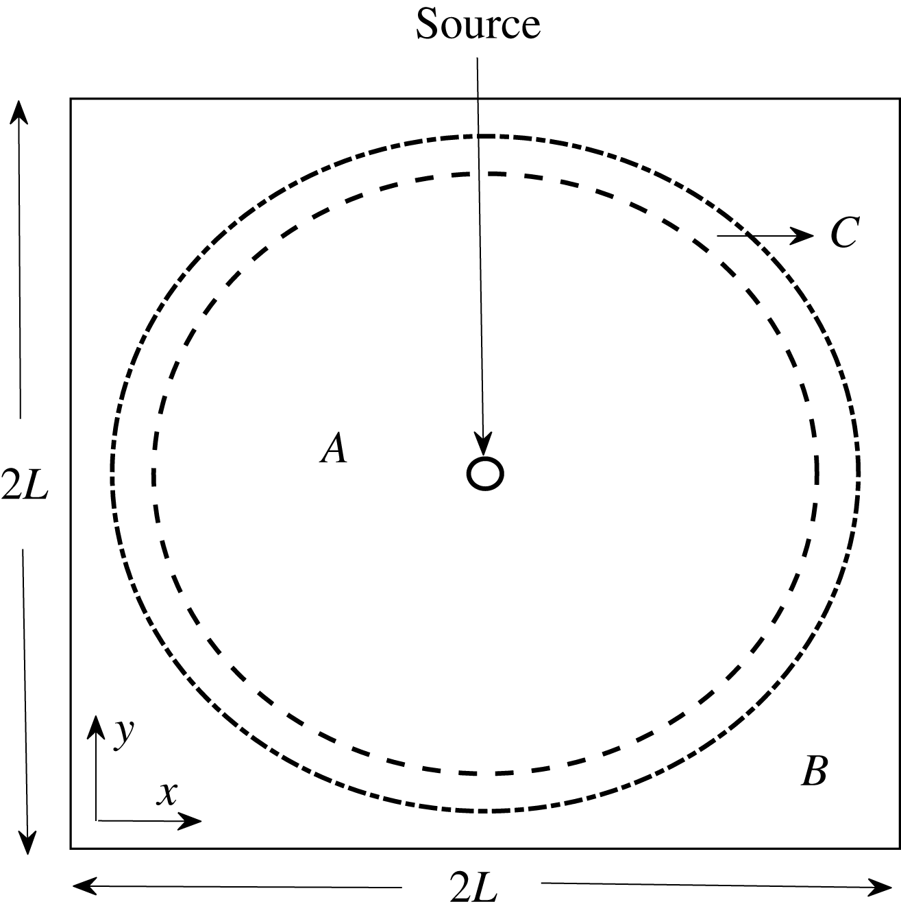
Schematic showing
 $A+B\xrightarrow[{}]{k}C$
in a radial source flow. Dashed curve represents miscible interface between fluids A and C, while dash-dotted curve represents the same between fluids B and C. The region between these curves shows the ring of product.

We consider a single phase fluid flow in a two-dimensional homogeneous, isotropic, saturated porous medium. We further assume that there exist two solutes
 $A$
and
 $B$
dissolved in a solvent and they produce a new solute
 $C$
by a second-order chemical reaction
 $A+B\xrightarrow[{}]{k}C.$
Without a loss of generality we call the solution of the solute
 $A$
in the solvent as fluid A, and similarly, fluid B and fluid C are defined as the solution of the solutes
 $B$
and
 $C$
respectively in the solvent. As shown schematically in figure 1, the fluid A is injected radially from a point source at the centre of the porous medium at a constant flow rate per unit depth,
 $Q$
, to displace the fluid B that initially saturates the porous medium. We assume that the three fluids are incompressible, Newtonian and neutrally buoyant – the gravitational forces are neglected in our model. The governing equations include Darcy’s law (Chen et al.
Reference Chen, Huang, Gadêlha and Miranda2008; Gérard & De Wit Reference Gérard and De Wit2009) for the fluid flow in a homogeneous porous medium:
 $$\begin{eqnarray}\displaystyle & \displaystyle \widetilde{\unicode[STIX]{x1D735}}\boldsymbol{\cdot }\widetilde{\boldsymbol{u}}=0, & \displaystyle\end{eqnarray}$$
 $$\begin{eqnarray}\displaystyle & \displaystyle \widetilde{\boldsymbol{u}}=-\frac{\unicode[STIX]{x1D705}}{\widetilde{\unicode[STIX]{x1D707}}(\widetilde{c})}\widetilde{\unicode[STIX]{x1D735}}\widetilde{p}, & \displaystyle\end{eqnarray}$$
 $\widetilde{\boldsymbol{u}}=(\widetilde{u},\widetilde{v})$
and
 $\widetilde{p}$
respectively denote the Darcy velocity and the fluid pressure,
 $\unicode[STIX]{x1D705}$
is the constant permeability of the porous medium.
 $\widetilde{a},\widetilde{b},\widetilde{c}$
, denote the concentration of the two reactants (
 $A,B$
) and the product (
 $C$
), respectively, and their mass balance satisfies the following system of coupled nonlinear partial differential equations (PDEs) (Gérard & De Wit Reference Gérard and De Wit2009; De Wit Reference De Wit2016):
 $$\begin{eqnarray}\displaystyle & \displaystyle \frac{\unicode[STIX]{x2202}\widetilde{a}}{\unicode[STIX]{x2202}\widetilde{t}}+(\widetilde{\boldsymbol{u}}\boldsymbol{\cdot }\widetilde{\unicode[STIX]{x1D735}})\widetilde{a}=\widetilde{\unicode[STIX]{x1D735}}\boldsymbol{\cdot }(D_{A}\widetilde{\unicode[STIX]{x1D735}}\widetilde{a})-k\widetilde{a}\widetilde{b}, & \displaystyle\end{eqnarray}$$
 $$\begin{eqnarray}\displaystyle & \displaystyle \frac{\unicode[STIX]{x2202}\widetilde{b}}{\unicode[STIX]{x2202}\widetilde{t}}+(\widetilde{\boldsymbol{u}}\boldsymbol{\cdot }\widetilde{\unicode[STIX]{x1D735}})\widetilde{b}=\widetilde{\unicode[STIX]{x1D735}}\boldsymbol{\cdot }(D_{B}\widetilde{\unicode[STIX]{x1D735}}\widetilde{b})-k\widetilde{a}\widetilde{b}, & \displaystyle\end{eqnarray}$$
 $$\begin{eqnarray}\displaystyle & \displaystyle \frac{\unicode[STIX]{x2202}\widetilde{c}}{\unicode[STIX]{x2202}\widetilde{t}}+(\widetilde{\boldsymbol{u}}\boldsymbol{\cdot }\widetilde{\unicode[STIX]{x1D735}})\widetilde{c}=\widetilde{\unicode[STIX]{x1D735}}\boldsymbol{\cdot }(D_{C}\widetilde{\unicode[STIX]{x1D735}}\widetilde{c})+k\widetilde{a}\widetilde{b}, & \displaystyle\end{eqnarray}$$
 $D_{A},D_{B},D_{C}$
are the diffusion coefficients of
 $A,B,C$
in the solvent, and
 $k$
is the reaction rate constant. The dynamic viscosity of the reactant fluids, fluid A and fluid B, are the same, and they differ from that of the product, fluid C. The viscosity of the fluids are modelled as an Arrhenius relation similar to the earlier works on reactive VF (Hejazi et al.
Reference Hejazi, Trevelyan, Azaiez and De Wit2010).
2.1 Non-dimensionalization
To be able to explicitly explore the effect of chemical reaction rate and the diffusion of the species (
 $A,B,C$
) on the dynamics, we employ for non-dimensionalization the characteristic length, time, velocity, solute concentration, viscosity and pressure, as
 $$\begin{eqnarray}\displaystyle \boldsymbol{x}=\frac{\widetilde{\boldsymbol{x}}}{\sqrt{Qt_{f}}},\quad t=\frac{\widetilde{t}}{t_{f}},\quad \boldsymbol{u}=\frac{\widetilde{\boldsymbol{u}}}{\sqrt{Q/t_{f}}}, & & \displaystyle\end{eqnarray}$$
 $$\begin{eqnarray}\displaystyle (a,b,c)=\frac{(\widetilde{a},\widetilde{b},\widetilde{c})}{a_{0}},\quad \unicode[STIX]{x1D707}=\frac{\widetilde{\unicode[STIX]{x1D707}}}{\unicode[STIX]{x1D707}^{\ast }},\quad p=\frac{\widetilde{p}}{Q\unicode[STIX]{x1D707}^{\ast }/\unicode[STIX]{x1D705}}. & & \displaystyle\end{eqnarray}$$
Here,
 $t_{f}$
is the final duration of the fluid injection. The characteristic viscosity
 $\unicode[STIX]{x1D707}^{\ast }$
is defined below. The resultant initial value problem written in dimensionless form satisfies coupled nonlinear partial differential equations:
 $$\begin{eqnarray}\displaystyle \unicode[STIX]{x1D735}\boldsymbol{\cdot }\boldsymbol{u}=0,\quad \boldsymbol{u}=-\frac{1}{\unicode[STIX]{x1D707}(c)}\unicode[STIX]{x1D735}p,\quad \unicode[STIX]{x1D707}(c)=\exp (R_{c}c), & & \displaystyle\end{eqnarray}$$
and
 $$\begin{eqnarray}\displaystyle \frac{\unicode[STIX]{x2202}a}{\unicode[STIX]{x2202}t}+(\boldsymbol{u}\boldsymbol{\cdot }\unicode[STIX]{x1D735})a=\frac{1}{Pe}\unicode[STIX]{x1D6FB}^{2}a-Da\,ab, & & \displaystyle\end{eqnarray}$$
 $$\begin{eqnarray}\displaystyle & \displaystyle \frac{\unicode[STIX]{x2202}b}{\unicode[STIX]{x2202}t}+(\boldsymbol{u}\boldsymbol{\cdot }\unicode[STIX]{x1D735})b=\frac{1}{Pe}\unicode[STIX]{x1D6FB}^{2}b-Da\,ab, & \displaystyle\end{eqnarray}$$
 $$\begin{eqnarray}\displaystyle & \displaystyle \frac{\unicode[STIX]{x2202}c}{\unicode[STIX]{x2202}t}+(\boldsymbol{u}\boldsymbol{\cdot }\unicode[STIX]{x1D735})c=\frac{1}{Pe}\unicode[STIX]{x1D6FB}^{2}c+Da\,ab, & \displaystyle\end{eqnarray}$$
associated with the initial conditions
 $$\begin{eqnarray}\displaystyle \boldsymbol{u}=(x[2\unicode[STIX]{x03C0}(x^{2}+y^{2})]^{-1},y[2\unicode[STIX]{x03C0}(x^{2}+y^{2})]^{-1}), & & \displaystyle\end{eqnarray}$$
and
 $$\begin{eqnarray}\displaystyle a(x,y,t=0)=\left\{\begin{array}{@{}ll@{}}1, & 0<x^{2}+y^{2}\leqslant d^{2}/4\\ 0, & \text{otherwise},\end{array}\right. & & \displaystyle\end{eqnarray}$$
 $$\begin{eqnarray}\displaystyle b(x,y,t=0)=1-a(x,y,t=0),\quad c(x,y,t=0)=0\quad \forall x,y, & & \displaystyle\end{eqnarray}$$
wherein
 $d$
is the dimensionless diameter of a circular region. The three dimensionless parameters appearing in equations (2.4a–c
)–(2.4f
) are
 $$\begin{eqnarray}\displaystyle R_{c}=\ln \left(\frac{\unicode[STIX]{x1D707}_{C}}{\unicode[STIX]{x1D707}^{\ast }}\right),\quad Da=\frac{t_{f}}{1/(ka_{0})},\quad Pe=\frac{Q}{D}, & & \displaystyle\end{eqnarray}$$
where
 $\unicode[STIX]{x1D707}^{\ast }=\unicode[STIX]{x1D707}(a+b=1,c=0)$
,
 $\unicode[STIX]{x1D707}_{C}=\unicode[STIX]{x1D707}(a+b=0,c=1)$
. Although, in general, the diffusion coefficients of the three species
 $A,B,C$
are different and not necessarily constant, we assume these to be identical and equal to a constant
 $D$
. This simplification allows us to focus on the understanding of the influence of a simple chemical reaction on the fingering instability in an otherwise stable miscible displacement. The definition of the Péclet number (
 $Pe$
) is similar to that used in experiments by Nagatsu et al. (Reference Nagatsu, Matsuda, Kato and Tada2007), which is a consequence of the scaling used, allowing a direct comparison with experiments. While
 $Pe$
determines the relative importance of the advection to the diffusion of the solute, the Damköhler number,
 $Da$
, is defined as the ratio of the advective time scale to the reaction time scale. A higher
 $Da$
corresponds to a smaller reaction time (a faster reaction rate) and hence the product is formed fast. Thus for every fixed
 $Pe$
, varying the two dimensionless parameters
 $Da$
and
 $R_{c}$
, we explore the effect of chemical reaction on fingering dynamics. Equations (2.4a–c
)–(2.4f
) are solved using a hybridization of a compact finite difference method and the pseudo-spectral method for the spatial derivative, while a fully explicit third-order Runge–Kutta method is used for the time integration (Chen et al.
Reference Chen, Huang, Gadêlha and Miranda2008, and refs. therein). Similar numerical schemes have been quite effective with the non-reactive counterparts, where good quantitative agreement with the theoretical results are available in the literature. To name a few, Chen & Meiburg (Reference Chen and Meiburg1998) reported a good agreement with the growth rate on a miscible interface, while for immiscible fluids, the number of fingers triggered (Chen, Huang & Miranda Reference Chen, Huang and Miranda2011, Reference Chen, Huang and Miranda2014) was found to be consistent with the theoretical results. We briefly discuss our method for the reactive miscible fluids below.
2.2 Numerical method
Numerical computations are performed in a square box
 $\unicode[STIX]{x1D6FA}=[-L,L]\times [-L,L]$
. In the absence of any viscosity gradient, the radial flow is a potential flow with velocity vector,
 $\boldsymbol{u}_{pot}=(x[2\unicode[STIX]{x03C0}(x^{2}+y^{2})]^{-1},y[2\unicode[STIX]{x03C0}(x^{2}+y^{2})]^{-1})$
. However, this potential flow is perturbed as the chemical reaction induces a viscosity variation at the miscible interface between the two reactants. In order to capture this deviation of the velocity from the potential flow velocity
 $\boldsymbol{u}_{pot}$
, we decompose the velocity vector at any time into two parts,
 $$\begin{eqnarray}\displaystyle \boldsymbol{u}=\boldsymbol{u}_{pot}+\boldsymbol{u}_{rot}. & & \displaystyle\end{eqnarray}$$
The singularity in the potential flow at the origin is regularized by introducing a Gaussian source of core
 $\unicode[STIX]{x1D70E}$
as in Chen et al. (Reference Chen, Huang, Gadêlha and Miranda2008):
 $$\begin{eqnarray}\displaystyle \boldsymbol{u}_{pot}=\left(\frac{(1-\text{e}^{-(x^{2}+y^{2})/\unicode[STIX]{x1D70E}^{2}})x}{2\unicode[STIX]{x03C0}(x^{2}+y^{2})},\frac{(1-\text{e}^{-(x^{2}+y^{2})/\unicode[STIX]{x1D70E}^{2}})y}{2\unicode[STIX]{x03C0}(x^{2}+y^{2})}\right), & & \displaystyle\end{eqnarray}$$
here
 $\unicode[STIX]{x1D70E}\leqslant d/2$
, the radius of the circle initially occupied by reactant
 $A$
. We take
 $d=0.15$
in all the simulations. Introducing a streamfunction
 $\unicode[STIX]{x1D713}$
such that
 $\boldsymbol{u}_{rot}=(\unicode[STIX]{x2202}\unicode[STIX]{x1D713}/\unicode[STIX]{x2202}y,-\unicode[STIX]{x2202}\unicode[STIX]{x1D713}/\unicode[STIX]{x2202}x)$
, we write the Darcy’s law, equation (2.4a–c
), by eliminating the pressure, as
 $$\begin{eqnarray}\displaystyle \unicode[STIX]{x1D6FB}^{2}\unicode[STIX]{x1D713}=-\unicode[STIX]{x1D714},\quad \unicode[STIX]{x1D714}=R_{c}[v(\unicode[STIX]{x2202}c/\unicode[STIX]{x2202}x)-u(\unicode[STIX]{x2202}c/\unicode[STIX]{x2202}y)]. & & \displaystyle\end{eqnarray}$$
We discretize the advection and diffusion terms in equations (2.4d )–(2.4f ) using fourth-order and sixth-order finite difference formulae (Lele Reference Lele1992) to obtain semi-discretized equations
 $$\begin{eqnarray}\displaystyle \unicode[STIX]{x2202}_{t}a=f(a,b,c),\quad \unicode[STIX]{x2202}_{t}b=g(a,b,c),\quad \unicode[STIX]{x2202}_{t}c=h(a,b,c), & & \displaystyle\end{eqnarray}$$
where
 $f,g,h$
are the discretized versions of the advection–diffusion–reaction operators corresponding to their continuous form in equations (2.4d
)–(2.4f
). No-flux boundary conditions are used for the solute concentrations and
 $\unicode[STIX]{x1D713}=0$
across all four boundaries. The equations (2.10) are associated with the initial conditions (2.5a
)–(2.5c,d
). For numerical convergence, the step-like initial condition is regularized as follows. Equation (2.5b
) tells us that the reactant
 $A$
is initially contained within a circle of radius
 $d/2$
, which is equivalent to a dimensionless diffusive time
 $t=d^{2}/8$
. Thus, the axisymmetric base state solution of Tan & Homsy (Reference Tan and Homsy1987) at
 $t=d^{2}/8$
is used as an initial condition for
 $a$
. We introduce a random disturbance of amplitude
 $\unicode[STIX]{x1D709}\sim O(10^{-2})$
around the points where
 $a=0.5$
, so that the concentration at those points is given as
 $a=0.5+\unicode[STIX]{x1D709}\sin (2\unicode[STIX]{x03C0}N),$
where
 $N$
is a random number between
 $0$
and
 $1$
. The same set of random numbers is used for all the simulations. The initial condition for
 $a$
subtracted from unity gives the initial condition for
 $b$
.
The system of equations (2.10) is solved using a fully explicit third-order Runge–Kutta method with adaptive time stepping that satisfies the Courant–Friedrichs–Lewy condition. Sixth-order compact finite difference approximations are used in equation (2.9) to compute
 $\unicode[STIX]{x1D714}$
. A fast and efficient solution of the Poisson equation in (2.9) is achieved using a hybridization of the compact finite difference and the pseudo-spectral methods. We employ a Galerkin-type discretization in the
 $x$
-direction and a sixth-order compact finite difference in the
 $y$
-direction for
 $\unicode[STIX]{x1D713}$
. The simulations are stopped as soon as the concentration near the boundary becomes more than
 $0.1$
for
 $a$
or less than
 $0.9$
for
 $b$
. In this study, we take
 $\unicode[STIX]{x1D6FA}=[-0.75,0.75]\times [-0.75,0.75]$
with
 $512\times 512$
grid points.
3 Results and discussions
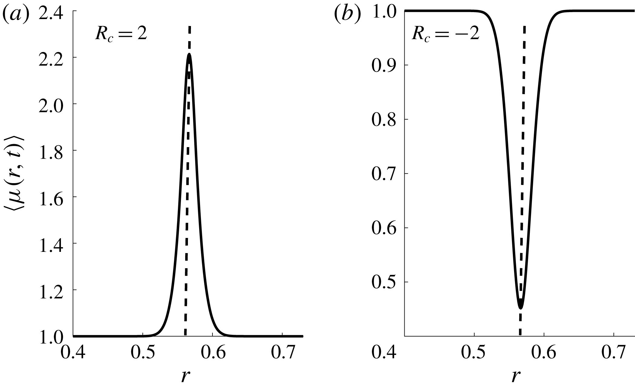
Viscosity profile across the interface (dashed line) along the radial direction for
 $Da=100,t=1$
.

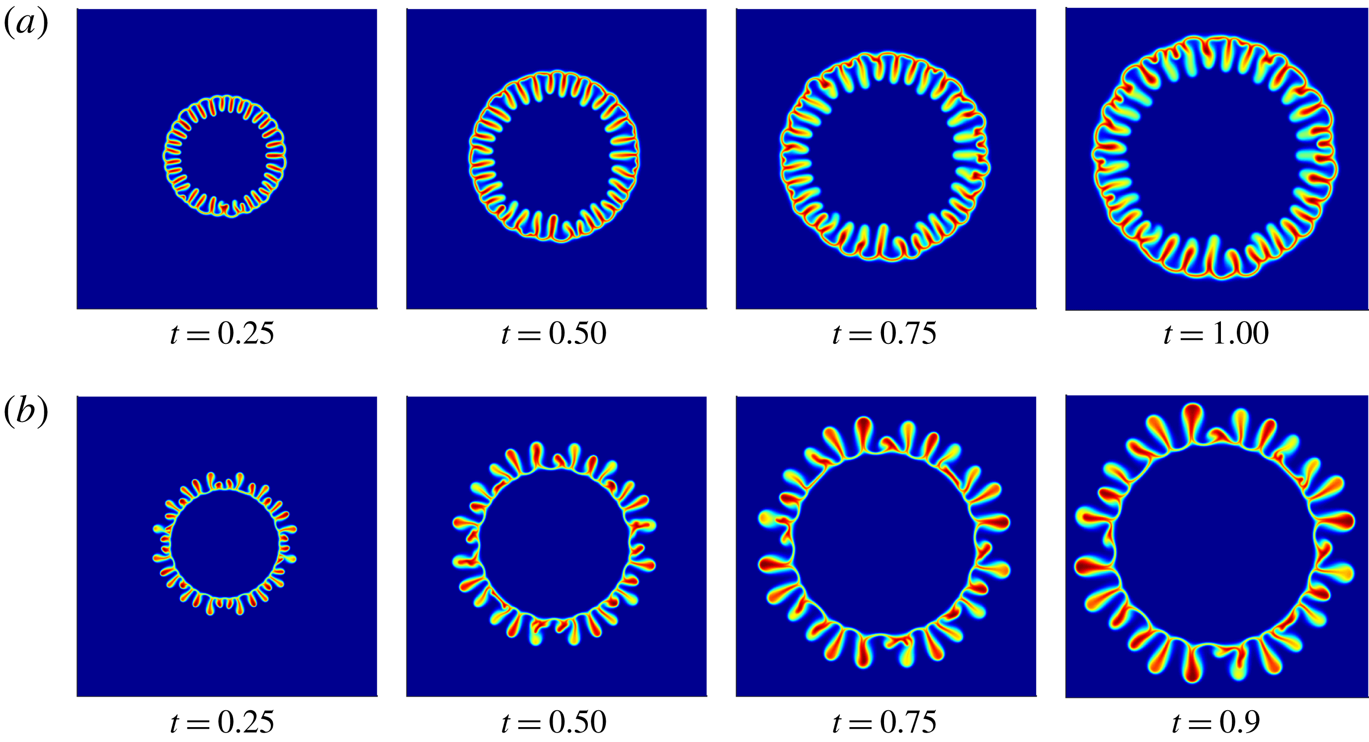
As mentioned in § 2, the dynamic viscosities of fluid A and fluid B are identical, which corresponds to a stable displacement in the absence of a chemical reaction or when the product viscosity is identical to that of the reactants. How does a chemical reaction alter this stable displacement if fluid C, formed due to the chemical reaction, has a viscosity different from the reactants? The product thus generated by the chemical reaction introduces a non-monotonicity in the viscosity profile, as shown in figure 2. Understanding the effect of the non-monotonicity can be of great help in controlling the instability. In figure 3, we show the temporal evolution of both a more as well as a less viscous product generated by the chemical reaction.
Temporal evolution of the concentration of product
 $C$
for
 $Da=100,Pe=3000,R_{c}=7$
(a) and
 $R_{c}=-7$
(b).

 $R_{c}>0$
corresponds to the case when the product viscosity is larger than the reactants. In this case, the viscosity
 $\unicode[STIX]{x1D707}(c)$
attains a local maximum at the reaction zone as shown in figure 2(a). For such viscosity profiles, the miscible interface between fluid A and fluid C is anticipated to be hydrodynamically unstable, whereas the miscible interface between fluid C and fluid B resists the growth of the fingers away from the source. As a consequence, the fingers form inside the ring of product observable in figure 3(a). Further, the tip of the outward growing fingers into the interface between fluid C and fluid B is wider than the root of the corresponding fingers. This is in good qualitative agreement with the viscosity increasing experiments (Nagatsu et al.
Reference Nagatsu, Matsuda, Kato and Tada2007; Riolfo et al.
Reference Riolfo, Nagatsu, Iwata, Maes, Trevelyan and De Wit2012) as well as the fan state fingering instability (Podgorski et al.
Reference Podgorski, Sostarecz, Zorman and Belmonte2007).
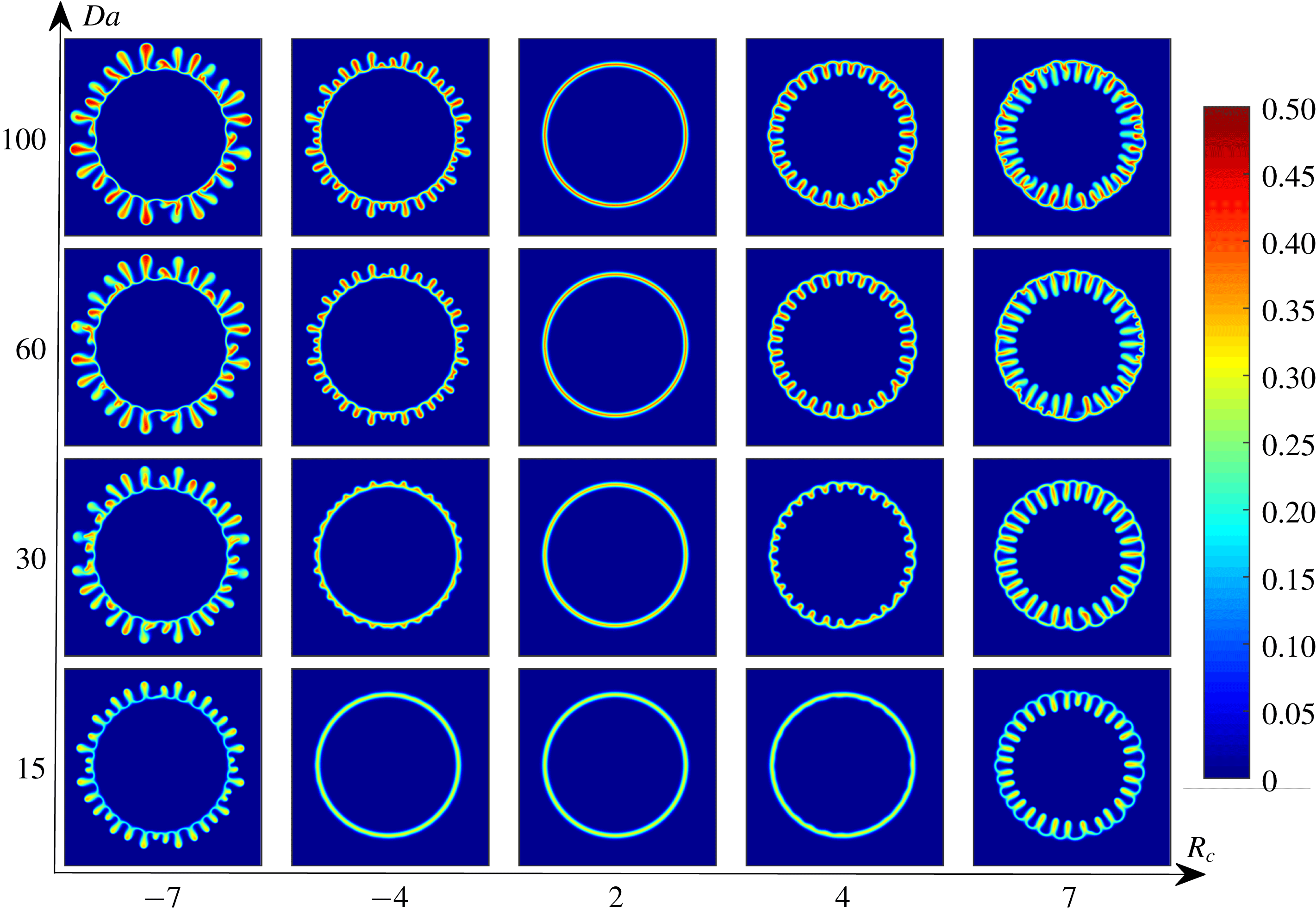
Density plots of the concentration of product
 $C$
for various
 $Da$
and
 $R_{c}$
and
 $Pe=3000$
at
 $t=0.9$
.

On the other hand, when the viscosity of the product is less than both the reactants, i.e.
 $R_{c}<0$
, the interface between fluid A and fluid C resists the growth of the fingers formed at the interface between fluid C and fluid B. The fingers develop at the outer interface of the ring of product and grow in the direction of the bulk fluid motion. Consequently, for larger
 $Da$
, the fingers quickly reach the boundary of the domain. In particular, for
 $R_{c}=-7$
and
 $Da=100$
, the outward fingers reach the domain boundary before
 $t=1$
and hence in figure 3(b), the temporal evolution is shown up to time
 $t=0.9$
only. The fingering patterns for
 $R_{c}<0$
are also in good qualitative agreement with existing experiments in the radial geometry (Riolfo et al.
Reference Riolfo, Nagatsu, Iwata, Maes, Trevelyan and De Wit2012). A comparison of the density plots for positive and negative
 $R_{c}$
, reveals that, for
 $R_{c}<0$
, the fingers are narrower away from source and hence cover a smaller area, another feature in good agreement with the experiments in which the reaction decreases the viscosity of the fluids locally (Nagatsu et al.
Reference Nagatsu, Matsuda, Kato and Tada2007).
The qualitative features depend on the sign of
 $R_{c}$
but the intensity and the interaction of fingers depend on the reaction rate too. Our numerical simulations reveal a variety of fingering patterns, which emerge due to a coupled effect of chemical reaction and hydrodynamics. In figure 4, we plot the reaction-induced fingering dynamics at
 $t=0.9$
for
 $Pe=3000$
and a wide range of
 $Da$
and
 $R_{c}$
, including both the cases of more and less viscous product forming reactions. For
 $Pe=3000,Da=60,100,R_{c}=-7$
, the fingers reach the boundary after
 $t=0.9$
, hence all the plots are shown at
 $t=0.9$
. For every
 $Da$
, an increasing finger interaction and vigorous fingering instability is evident as
 $|R_{c}|$
increases. This is in qualitative agreement with the linear stability results of Hejazi et al. (Reference Hejazi, Trevelyan, Azaiez and De Wit2010) for viscosity-matched reactants. Depending on
 $Da$
, a stable displacement even for an unfavourable viscosity contrast between the displacing and displaced fluid is a novel finding of our work. Also for
 $Da=15,R_{c}=4$
bumps are visible which are absent for
 $R_{c}=-4$
. Thus, a reaction producing a more viscous product is more unstable. We explain this in the next subsection § 3.1.
3.1 Quantitative analysis
For the quantitative analysis, we make the transformations from
 $(x,y)$
coordinates to
 $(r,\unicode[STIX]{x1D703})$
coordinates. The conversions are made from
 $r=\unicode[STIX]{x1D70E}$
to
 $r=L$
in order to avoid the effect of a Gaussian source, if any, near the origin. So the domain in the
 $(r,\unicode[STIX]{x1D703})$
coordinates is
 $[\unicode[STIX]{x1D70E},L]\times [0,2\unicode[STIX]{x03C0})$
. We carry the quantitative analysis in the
 $(r,\unicode[STIX]{x1D703})$
plane in the next two subsections §§ 3.1.1 and 3.1.2.
3.1.1 Onset of instability
Interfacial length is the length of the product ring for a stable displacement and the length of the curve along the fingering pattern for an unstable displacement. In order to quantify the interfacial length, we define it in the
 $(r,\unicode[STIX]{x1D703})$
plane as,
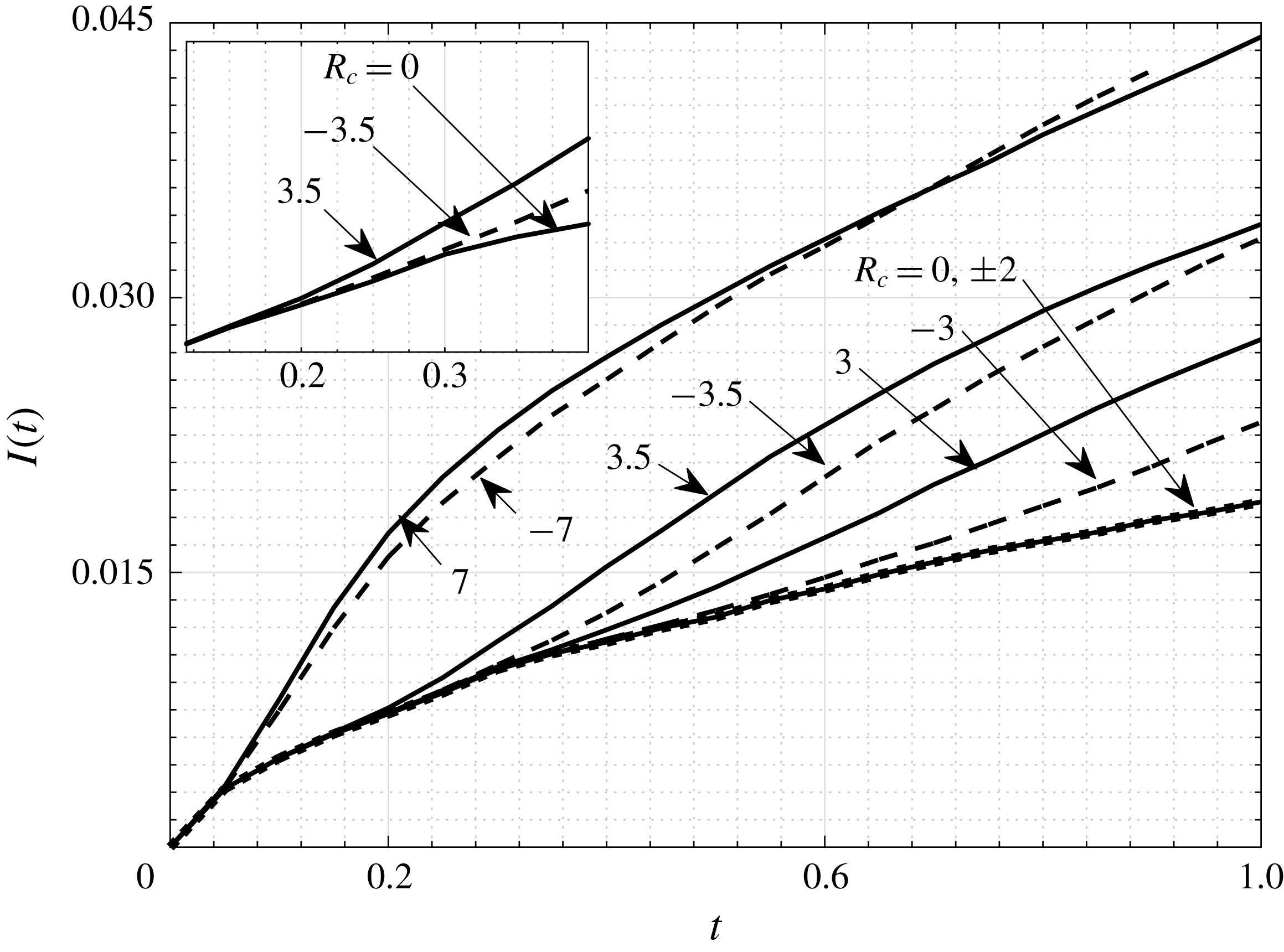
 $$\begin{eqnarray}\displaystyle I(t)=\int _{\unicode[STIX]{x1D70E}}^{L}\int _{0}^{2\unicode[STIX]{x03C0}}\sqrt{\left(\frac{\unicode[STIX]{x2202}c}{\unicode[STIX]{x2202}r}\right)^{2}+\frac{1}{r^{2}}\left(\frac{\unicode[STIX]{x2202}c}{\unicode[STIX]{x2202}\unicode[STIX]{x1D703}}\right)^{2}}r\,\text{d}\unicode[STIX]{x1D703}\,\text{d}r. & & \displaystyle\end{eqnarray}$$
The numerical integration is carried out using the trapezoidal rule. In the
 $(r,\unicode[STIX]{x1D703})$
plane,
 $\text{d}r$
is fixed by the spatial discretization in the
 $(x,y)$
plane as
 $\text{d}r=\sqrt{\text{d}x^{2}+\text{d}y^{2}}$
but
 $\text{d}\unicode[STIX]{x1D703}=\tan ^{-1}(\text{d}y/\text{d}x)$
results in a poor discretization. So, we fix
 $\text{d}\unicode[STIX]{x1D703}=10^{-4}$
and carry out the conversions from the
 $(x,y)$
to the
 $(r,\unicode[STIX]{x1D703})$
plane. It is verified that decreasing
 $\text{d}\unicode[STIX]{x1D703}$
further does not qualitatively or quantitatively change our results.
 $I(t)$
normalized with
 $d\unicode[STIX]{x1D703}$
is shown in figure 5.
Interfacial length as a function of time for
 $Da=100,Pe=3000$
and various
 $R_{c}$
. Inset shows zoomed plot around time
 $t\in (0.04,0.44)$
in order to highlight the onset time for
 $R_{c}=3.5$
and
 $R_{c}=-3.5$
. Clearly, the instability is triggered late for
 $R_{c}=-3.5$
.

 $I(t)$
can be used as a tool to gain an insight into the onset of instability. The instant, when
 $I(t)$
for
 $R_{c}\neq 0$
departs from that for
 $R_{c}=0$
, is the time when instability triggers and is termed the onset time. It is observable from figure 5 that the difference between the onset time for
 $R_{c}<0$
and the corresponding positive
 $R_{c}$
decreases as we increase
 $|R_{c}|$
and ultimately the onset times become equal. This is because, before fingering occurs, the product is formed in a ring and the difference in onset time is attributed to the fluid velocity at the unstable interface of the ring of product. For
 $R_{c}<0$
, fingers are formed at the outer interface of the ring, where the fluid velocity of the unperturbed flow is smaller than the velocity at the inner interface of the product ring. Therefore the advective force, which is responsible for the fingering instability, is weaker in the former case. As
 $|R_{c}|$
increases, the onset time of instability decreases and it is independent of width of the ring. Hence for a given
 $Da$
, onset time for
 $R_{c}<0$
is always less than, or equal to, that for the corresponding positive
 $R_{c}$
. This is in contradiction to the linear stability analysis in a rectilinear geometry (Hejazi et al.
Reference Hejazi, Trevelyan, Azaiez and De Wit2010) and can be attributed to the spatially varying velocity of the potential flow. Thus the geometry used for the nonlinear simulations does play a role in the dynamics and can lead to different results. Also,
 $I(t)$
for many non-zero
 $R_{c}$
coincides with that for
 $R_{c}=0$
for all times. This restates the existence of stable flows for a range of
 $R_{c}$
despite an unfavourable viscosity contrast.
3.1.2 Effect of barrier
It is evident from figure 2 that the non-monotonicity introduced in the viscosity profile by the chemical reaction results in a hydrodynamically stable interface where a more viscous fluid displaces a less viscous one. The stable interface hinders the fingers growing at the other interface. This is observable from the density plots in figure 4 where the fingers either only grow inwards for
 $R_{c}>0$
or outwards for
 $R_{c}<0$
. In order to quantify the effect of the barrier, we define the angular average concentration as
 $$\begin{eqnarray}\displaystyle \langle c(r,t)\rangle =(2\unicode[STIX]{x03C0})^{-1}\int _{0}^{2\unicode[STIX]{x03C0}}c(r,\unicode[STIX]{x1D703},t)\,\text{d}\unicode[STIX]{x1D703}. & & \displaystyle\end{eqnarray}$$
This quantification is possible only due to the transformation from the
 $(x,y)$
to
 $(r,\unicode[STIX]{x1D703})$
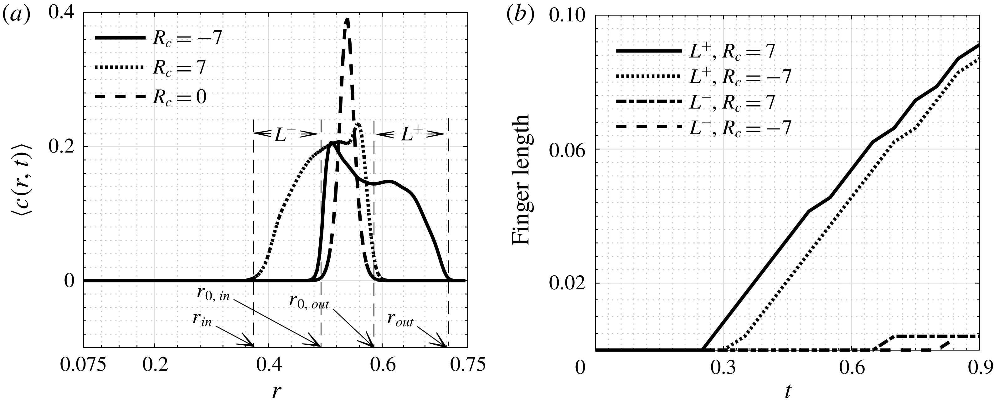
plane. Figure 6
(a) shows
 $\langle c(r,t)\rangle$
at
 $t=0.9$
for various
 $R_{c}$
and
 $Da=100,Pe=3000$
. The bumps towards the left for
 $R_{c}=7$
and towards the right for
 $R_{c}=-7$
show that fingers predominantly grow inwards and outwards, respectively for positive and negative
 $R_{c}$
. Further, we use
 $\langle c(r,t)\rangle$
to find the length of the fingers. We define the fingers growing at the outer interface of the product ring as outward fingers while the fingers at the inner interface are defined as inward fingers. To analyse the effect of the barrier induced by the chemical reaction, we define the outward and the inward finger lengths as
 $$\begin{eqnarray}\displaystyle L^{+}=|r_{0,out}-r_{out}|\quad \text{and}\quad L^{-}=|r_{0,in}-r_{in}|, & & \displaystyle\end{eqnarray}$$
respectively. Here,
 $r_{0,in}$
and
 $r_{0,out}$
are the radii when
 $\langle c(r,t)\rangle \approx 10^{-4}$
for
 $R_{c}=0$
as shown in figure 6(a) and
 $r_{in}$
and
 $r_{out}$
are the corresponding values for
 $R_{c}\neq 0$
. Figure 6(b) shows
 $L^{+}$
is larger (smaller) than
 $L^{-}$
for negative (positive)
 $R_{c}$
, thus capturing the effect of the barrier introduced by the non-monotonicity, on the finger length.
(a) Angular average concentration,
 $\langle c(r,t)\rangle$
at
 $t=0.9$
for
 $Da=100,Pe=3000$
and various
 $R_{c}$
.
 $r_{0,in}$
,
 $r_{0,out},r_{in}$
and
 $r_{out}$
used to compute
 $L^{+}$
and
 $L^{-}$
are also shown. (b) Outward and inward finger lengths respectively for
 $R_{c}=-7$
and 7 for
 $Da=20$
.

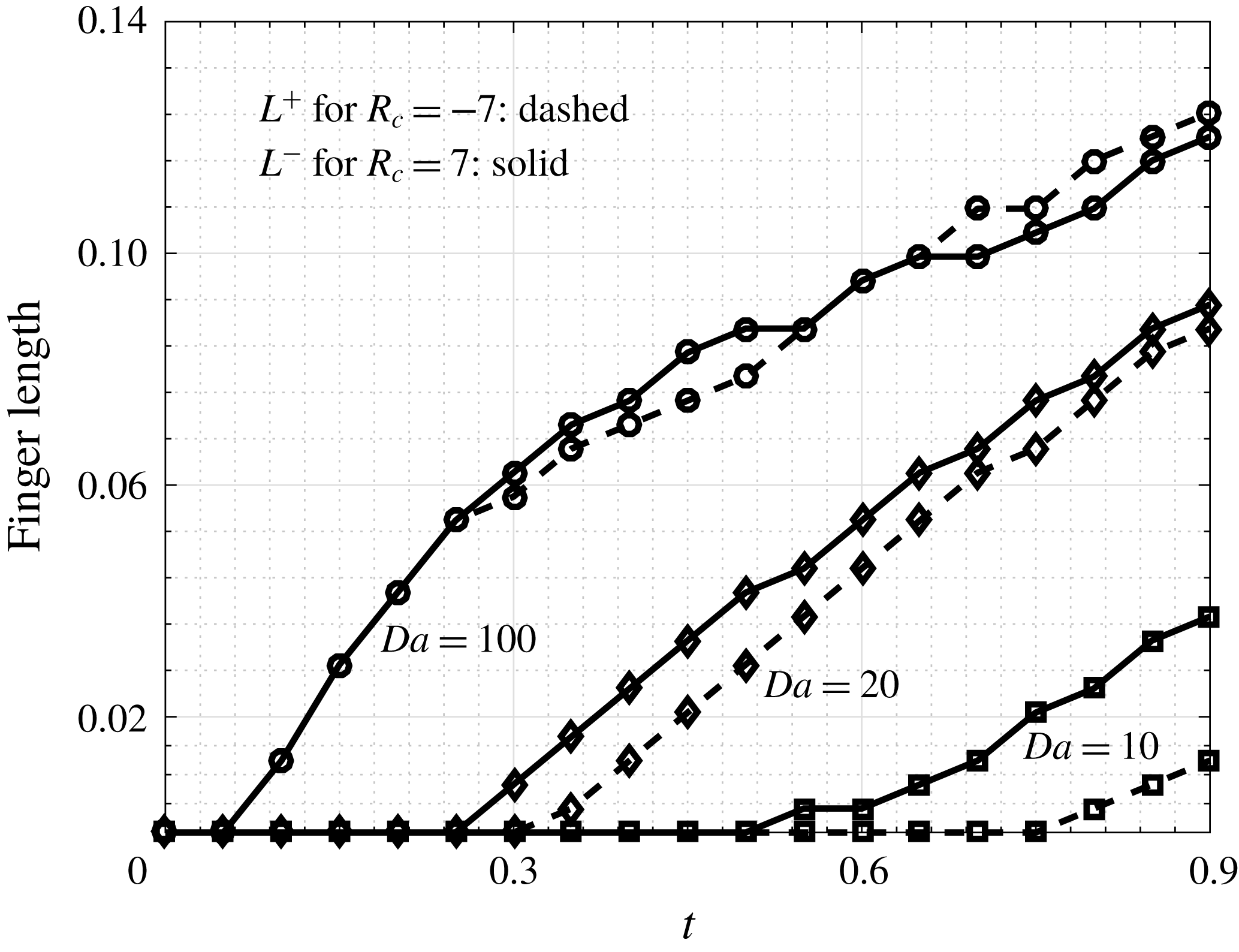
Outward and inward finger lengths respectively for
 $R_{c}=-7$
and 7 for
 $Da=100$
, 20 and 10.

We capture the effect of the chemical reaction on the finger length in figure 7. It is clear that a reaction producing a more viscous product is more unstable as the length of the fingers for positive
 $R_{c}$
is always more than that for corresponding
 $R_{c}<0$
, for fixed
 $Da$
. This is due to the radially varying potential component of velocity which delays the onset and consequently reduces the finger length for
 $R_{c}<0$
. Further, as
 $Da$
increases, the two finger lengths are found to approach each other, with
 $L^{-}$
ultimately surpassing
 $L^{+}$
. This is attributed to the barrier in the direction of bulk fluid motion for positive
 $R_{c}$
which hinders the growth of the fingers.
3.2 Critical
 $R_{c}$
for the fingering instability

The above discussions reveal that, for each
 $Da$
, a minimum viscosity contrast is required for the fingering instability to occur. To determine the critical parameters for the fingering instability, we use the interfacial length corresponding to
 $R_{c}=0$
as the reference. A set of parameters (
 $Da,R_{c}$
) is assigned an unstable displacement if the corresponding interfacial length exceeds the reference value by more than
 $5\,\%$
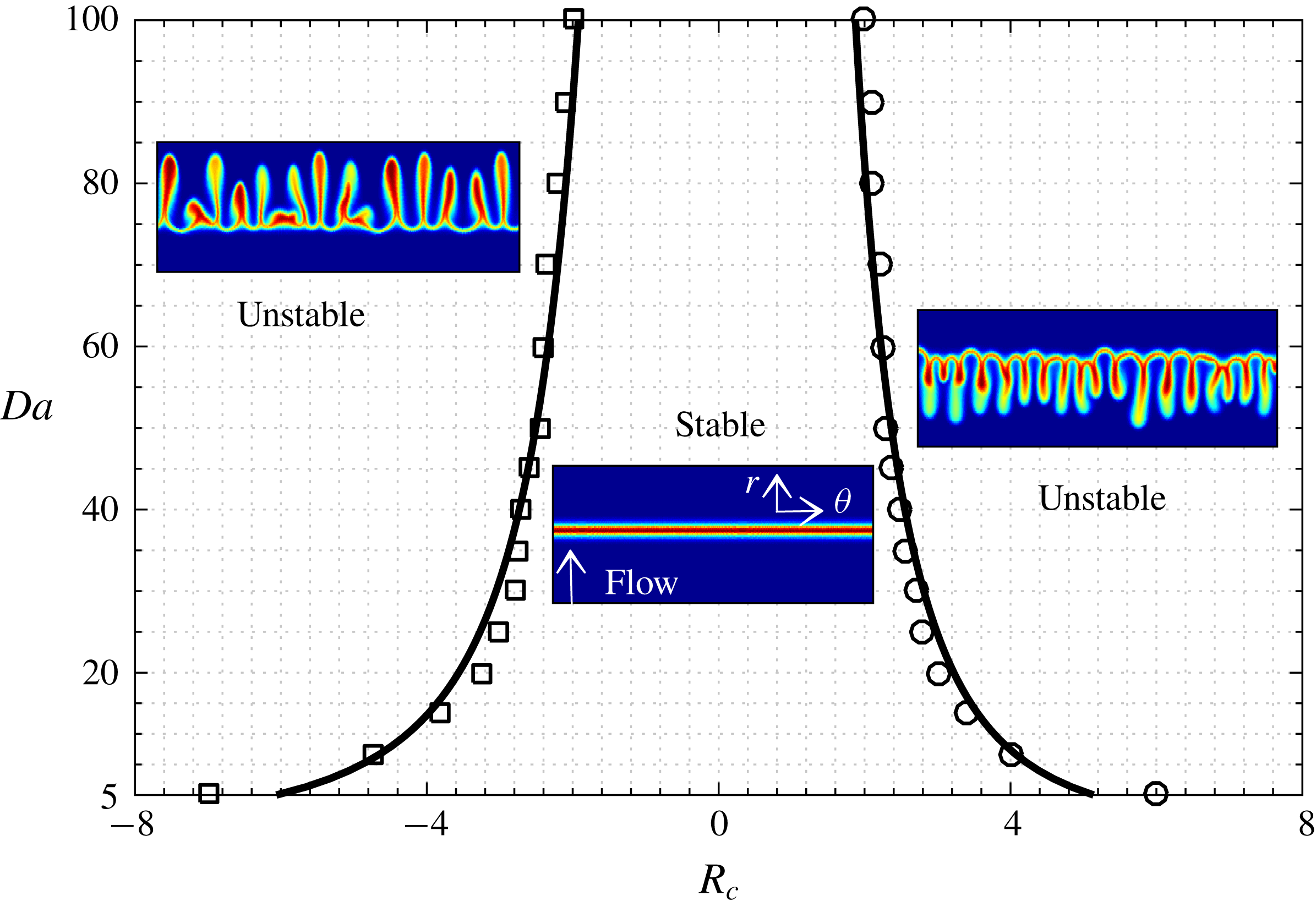
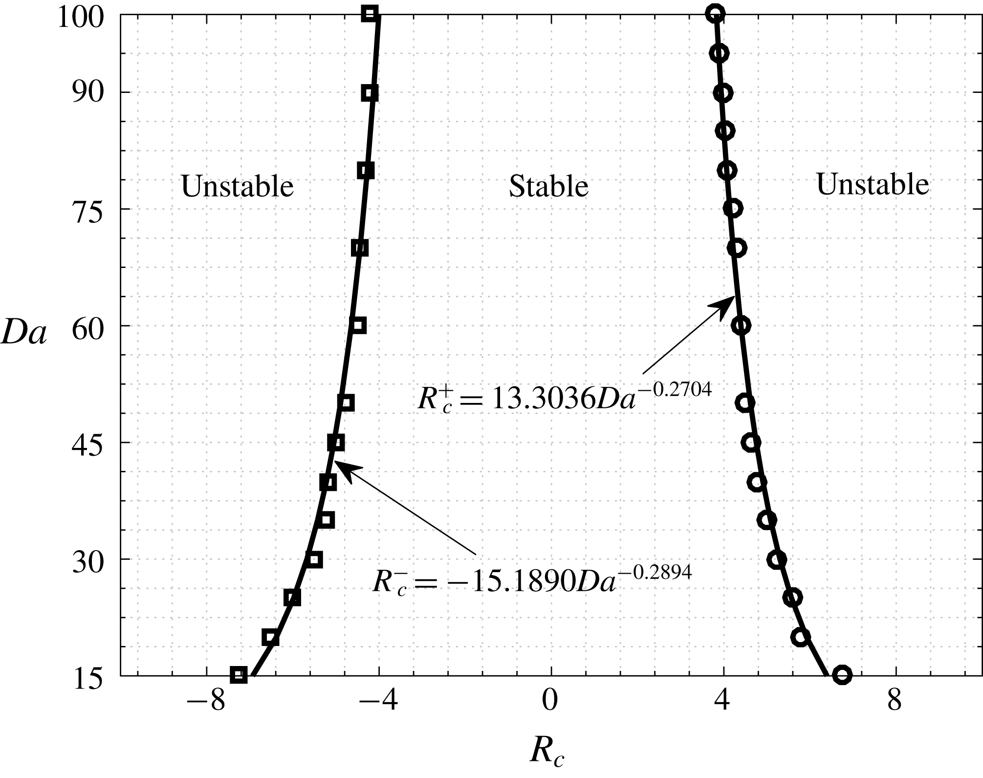
; otherwise it is assigned as a stable displacement. Thus obtained stable and unstable cases are summarized in figure 8 for
 $Pe=3000$
, which depicts that the
 $Da-R_{c}$
plane consists of a stable region around
 $R_{c}=0$
, sandwiched between two unstable regions. This stable region exists for all
 $Da$
values considered and narrows as
 $Da$
increases. Therefore, for every finite
 $Da$
, we capture critical values of
 $R_{c}$
denoted as
 $R_{c}^{-}$
and
 $R_{c}^{+}$
, such that no VF occurs when
 $R_{c}^{-}\leqslant R_{c}\leqslant R_{c}^{+}$
and VF is observed outside this interval. Symbols in figure 8 denote the critical parameters
 $R_{c}^{-}$
(squares),
 $R_{c}^{+}$
(circles), while the lines represent a least squares fit to the function
 $|R_{c}^{\pm }|\propto Da^{-\unicode[STIX]{x1D6FD}_{\pm }}$
. A naive observation to be made here is that a higher viscosity gradient is required to trigger the instability for the reaction producing a less viscous product as
 $|R_{c}^{-}|>|R_{c}^{+}|$
for all
 $Da$
. The numerical simulations are carried out for a wide range of
 $Pe$
and the qualitative results presented in figure 8 remain unaffected for other values of
 $Pe$
as well, as is evident from the
 $Da-R_{c}$
parameter space for
 $Pe=1000$
in figure 9. It is verified that the stable region reduces as
 $Pe$
increases, but never completely disappears.
 $Da-R_{c}$
parameter space showing stable as well as unstable regions for
 $Pe=3000$
. ▫ denote
 $R_{c}^{-}$
and ○ denote
 $R_{c}^{+}$
, while the solid lines represent the power laws
 $R_{c}^{+}=8.8318Da^{-0.3365}$
and
 $R_{c}^{-}=-11.2329Da^{-0.3833}$
. The truncated density plots of product concentration in
 $(r,\unicode[STIX]{x1D703})$
coordinates representing each zone are also shown in the inset.

Widening of the stable region on decreasing
 $Pe$
.
 $Da-R_{c}$
parameter space for
 $Pe=1000$
with the solid lines representing the power laws
 $|R_{c}^{\pm }|=\unicode[STIX]{x1D6FC}_{\pm }Da^{-\unicode[STIX]{x1D6FD}_{\pm }}$
. Critical
 $R_{c}$
is shown by symbols with ▫ and ○ respectively denoting
 $R_{c}^{-}$
and
 $R_{c}^{+}$
.

Now, we give a relation between the critical parameters so as to mathematically determine the bounds of the stable region for any given moderate
 $Da$
. Bischofberger, Ramachandran & Nagel (Reference Bischofberger, Ramachandran and Nagel2014) experimentally determined the existence of a critical viscosity contrast (
 $R_{crit}$
) for the fingering instability to occur in the miscible VF. Following the stability analysis of the fingering instability, we can write the critical viscosity ratio as
 $\unicode[STIX]{x1D707}_{crit}\approx \text{e}^{R_{crit}}$
. We extend this idea for the current case of reactive fingering instability in miscible fluids. We write the critical viscosity
 $\unicode[STIX]{x1D707}_{crit}^{\pm }$
as
 $\text{e}^{|R_{c}^{\pm }|f(Da)}$
, where
 $f(Da)$
is a function of
 $Da$
, to be determined. Setting
 $\unicode[STIX]{x1D707}_{crit}^{\pm }=\unicode[STIX]{x1D707}_{crit}$
and using a best fit of the numerically obtained critical parameter, we obtain
 $$\begin{eqnarray}\displaystyle R_{c}^{+}=\unicode[STIX]{x1D6FC}_{+}Da_{c}^{-\unicode[STIX]{x1D6FD}_{+}},\quad R_{c}^{-}=-\unicode[STIX]{x1D6FC}_{-}Da_{c}^{-\unicode[STIX]{x1D6FD}_{-}}, & & \displaystyle\end{eqnarray}$$
where
 $\unicode[STIX]{x1D6FC}_{\pm }$
and
 $\unicode[STIX]{x1D6FD}_{\pm }$
are the fitting parameters which depend on
 $Pe$
. These parameters for
 $Pe=3000,1000$
are given in figures 8 and 9, respectively. Clearly the stable region widens on decreasing
 $Pe$
. This clearly is a consequence of the effect of the stabilizing diffusive force on miscible VF. Thus, for a given
 $Pe$
, we can divide the
 $Da-R_{c}$
parameter space into three regions which can be used for suitably choosing the parameters to control VF.
4 Conclusion
With an aim to explore the effect of the chemical reaction and geometry on VF, we numerically studied the dynamics of chemical reaction-induced fingering instabilities in miscible radial displacements. We choose a pair of viscosity-matched reactants, such that in the absence of a chemical reaction one stably displaces other. Thus, the chemical reaction induces a non-monotonic viscosity variation radially. We have explored a range of parameter values covering a wide spectrum of reaction rates and cases of viscosity increasing as well as viscosity decreasing chemical reactions. Depending on the viscosity of the end product, either the inner or the outer interface of the product ring becomes unstable, provided the viscosity contrast between the displacing and the displaced fluid is larger than a critical value. The instability of the inner and outer interfaces of the product is summarized in a parameter space spanned by
 $R_{c}$
and
 $Da$
. Our results show that a non-zero viscosity contrast is not sufficient for VF to occur, which is also true for the classical miscible fingering instability in non-reactive fluids (Bischofberger et al.
Reference Bischofberger, Ramachandran and Nagel2014). We have shown that fingering instability occurs when the mobility ratio exceeds a critical value, which depends on both
 $Da$
and
 $Pe$
. Depending on these critical parameter values, for a fixed
 $Pe$
, the
 $R_{c}$
–
 $Da$
parameter space is divided into three regions – one stable region separating two unstable regions. For a given
 $Pe$
, the critical log-mobility ratios and the critical Damköhler number are found to follow a power law. The stable region exists for all
 $Pe$
, with its the width being dependent on
 $Pe$
.
Fingering dynamics observed in the unstable regions of the
 $Da-R_{c}$
parameter space is in good qualitative agreement with the experiments. Besides triggering VF, the chemical reaction also introduces a barrier to the fingers. A delayed onset of VF for
 $R_{c}<0$
in comparison to that for
 $R_{c}>0$
is a result of the coupled effect of the stable barrier and a decaying
 $\boldsymbol{u}_{pot}$
. This is exactly opposite to the predictions from linear stability theory in a rectilinear flow (Hejazi & Azaiez Reference Hejazi and Azaiez2010). Thus, there is a need to consider more theoretical and numerical studies on miscible reactive VF in a radial geometry. Furthermore, our numerically predicted
 $Da-R_{c}$
parameter plane can be accessed to control VF by suitably choosing the reactants and the reaction. We believe more experiments will be conducted to improve the numerically predicted boundary between the adjacent regions.
Acknowledgements
M.M. acknowledges the financial support from SERB, Government of India through project grant no. MTR/2017/000283. S.P. acknowledges the support of the Swedish Research Council Grant no. 638-2013-9243. C.-Y.C. is thankful to ROC (Taiwan) Ministry of Science and Technology, for financial support through Grant no. MOST 105-2221-E-009-074-MY3. V.S. and M.M. thank Y. Nagatsu for various fruitful discussions. V.S. also acknowledges 2017 NCTU Taiwan Elite Internship Program for the financial support to visit C.-Y.C.