1 Introduction
1.1 Turbulence and layers
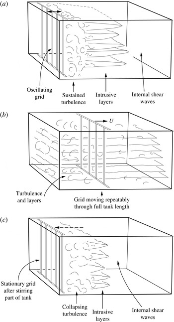
The effect and properties of turbulence in a stratified fluid are of fundamental importance in the study of environmental fluid dynamics. In the hope of clarifying the basic physical processes, numerous laboratory experiments have been made and reported in which turbulence is generated in stratified fluids by moving grids spanning the width and depth of a laboratory tank. By some yet undetermined means, turbulence sometimes leads to the formation of multiple horizontal layers of relatively uniform density within a fluid that, initially, is uniformly stratified (i.e. of constant buoyancy frequency,
 $N$
). As sketched in figure 1, the layers occur in three different types of experiment, (a–c), in which vertical grids move horizontally through the uniformly stratified fluid. In type (a), intrusive layers spread from a horizontally localised region where it is continuously generated by a grid oscillating with frequency,
 ${\it\omega}$
, typically
 ${\sim}10N$
. The grid may be located at the end of a tank as in figure 1(a) or in the centre as in figure 2. In type (b) experiments the grid moves at constant speed,
 $U$
, back and forth throughout the length of a rectangular tank with relatively lower frequency
 ${\it\omega}\sim 0.1N$
. Layers are apparent when the grid motion is temporally stopped. In type (c) experiments a ‘cloud’ of turbulence decays after a short period of horizontally localized grid mixing. Layers develop as intrusions from the turbulent cloud. The layers in some of the experiments are sometimes remarkably uniform and periodic in the vertical, e.g. as observed in type (a) experiments by Browand, Guyomar & Yoon (Reference Browand, Guyomar and Yoon1987; see especially their figure 15) or in type (b) experiments by Ruddick, Mcdougall & Turner (Reference Ruddick, Mcdougall and Turner1989, figure 4d). Internal waves are observed to propagate ahead of the intrusions in experiments of type (a) and (c). Horizontal ‘pancake’ vortices related to the generation vortical modes are found in the late stages of some experiments (see e.g. Praud, Fincham & Sommeria Reference Praud, Fincham and Sommeria2005), but are left for consideration elsewhere.
A sketch of layers formed in the three types of laboratory experiments, (a–c). In (a) the grid oscillates sinusoidally with amplitude much less than the tank length and with frequency much exceeding the buoyancy frequency,
 $N$
. In (b) the grid repeatedly moves back and forth at constant speed through the whole length of the tank with frequency comparable to or less than
 $N$
. In (c) the grid moves rapidly over a distance shorter than the tank length and stops, leaving a collapsing region of turbulence. Internal shear waves propagate ahead of the intrusive layers in (a) and (c).

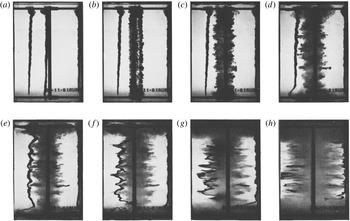
The development of horizontally spreading intrusions forming a layered structure in an experiment of type (a) in which a grid of vertical bars oscillates continuously in the centre of a tank filled with uniformly stratified salt solution. The grid, with solidarity parameter,
 $S\,(=b/M),=0.34$
, is viewed from the side. In parts (a) and (b) three columns of dye can be seen that were added before the grid motion was started at time,
 $t=0$
. One is close to the grid, one is on the right wall of the tank and the other half-way between the grid and the left wall. The width of the images is the tank width, 20.3 cm. The amplitude of grid motion,
 $a=0.94~\text{cm}$
, its frequency,
 ${\it\omega}=21.3~\text{rad}~\text{s}^{-1}$
and the buoyancy frequency,
 $N=1.98~\text{rad}~\text{s}^{-1}$
. The photos are at non-dimensional times,
 $Nt$
, of (a) 0, (b) 0.99, (c) 2.77, (d) 6.34, (e) 10.7, (f) 22.0, (g) 39.8, (h) 113.5. The horizontal separation of the noses of the intrusions and the third column of dye is insufficient to distinguish between the vertical structures of the waves and the intrusions even at moderate values of times,
 $Nt$
. (From Thorpe (Reference Thorpe1982, figure 3).)

Our purpose is, by synthesising and comparing existing laboratory and numerical studies, to examine the possible mechanisms that produce layers and to explain their vertical scale. The formation of layers by turbulence has attracted the attention of oceanographers seeking to explain the fine-scale density structure of the ocean. Whilst single layers are formed by the diapycnal mixing of a breaking internal wave, several mechanisms (including double-diffusive convection; Turner Reference Turner1973) are known to cause multiple layers. Layers form as intrusions (Manins Reference Manins1976) from a density current flowing down a sloping boundary (e.g. Baines Reference Baines2001; Snow & Sutherland Reference Snow and Sutherland2014). They may also be caused by turbulent mixing on a slope (Thorpe Reference Thorpe and Imberger1998; the vertical size of layers observed by Inall (Reference Inall2009) in Loch Etive, Scotland, appears, however, to be associated with the scale of roughness on an adjoining slope rather than with that of turbulence, e.g. the Ozmidov overturning scale, on a uniform slope). Layers are sometimes transient, moving vertically through the density field, a consequence of internal wave packets propagating through and straining a background density (e.g. Lazier Reference Lazier1973; Alford & Gregg Reference Alford and Gregg2001). Whilst yet to be observed either in the laboratory or in the natural environment, layers might also be formed by the successive breaking of internal waves in a wave group as it propagates upwards or downwards through a stratified environment (Thorpe Reference Thorpe1999). Although ostensibly the fluid motions and layers produced by a grid in the laboratory have little immediate relevance to the ocean (or to lakes or the atmosphere), the grid experiments offer information about the time scale and nature of the collapse of turbulence and provide insight into processes that may act in the natural environment. A relationship between layers and internal waves may be the most significant common factor.
1.2 Grid mixing
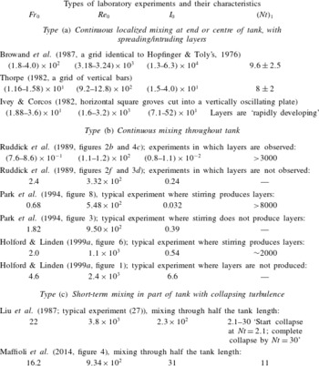
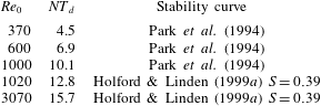
Relevant laboratory experiments of the three types are summarized in table 1. The grids vary from a single vertical cylinder moving steadily from end to end of a tank (Park, Whitehead & Gnanadeskian Reference Park, Whitehead and Gnanadeskian1994) to a set of parallel vertical bars that oscillates continually through a short distance along the tank (Thorpe Reference Thorpe1982) or oscillates once at steady speed through part of the length of the tank (Maffioli et al. Reference Maffioli, Davidson, Dalziel and Swaminathan2014). More complex grids are used, e.g. vertical bars mounted 6 cm apart along the 4 m length of the tank on strips spaced 3 cm laterally that can be oscillated longitudinally with opposite phase for alternate strips (Ruddick et al. Reference Ruddick, Mcdougall and Turner1989).
Typical parameter values in three types of laboratory experiments in which a uniformly stratified fluid is stirred by moving grids. The initial Froude number,
 $Fr_{0}=U/Nb$
(see (1.1)). The Reynolds number,
 $Re_{0}=Ul/{\it\nu}$
(see (1.2)). The parameter,
 $I_{0}=1.25\times 10^{-4}Re_{0}Fr_{0}^{2}$
is a measure of the turbulent buoyancy Reynolds number as defined in § 1.2.
 $(Nt)_{\text{l}}$
gives the approximate non-dimensional time,
 $Nt$
, at which layers are found or, in type (a) and (c) experiments, intrusive layers first appear. In most experiments grids composed of vertical bars are used to avoid generating internal waves or setting a vertical scale for the layers. Exceptions are Ivey & Corcos (Reference Ivey and Corcos1982) who use a plate with horizontal ridges and Browand et al. (Reference Browand, Guyomar and Yoon1987) who use a square-mesh grid (in some experiments set obliquely at 45° to the horizontal but seemingly with no effect on the intrusion scales). The experiments of type (a) covered by the shown values are those listed in table 3. For types (b) and (c) the sources of data are given with the authors. The ratio,
 $S=$
 $b/M=0.39$
in both the listed experiments of Holford & Linden (Reference Holford and Linden1999a
).

Some related experiments are not discussed here. These include Itsweire, Helland & van Atta (Reference Itsweire, Helland and van Atta1986) in which a 10-layer flow passes through a stationary grid, and Britter et al. (Reference Britter, Hunt, Marsh and Snyder1983) and Xiang et al. (Reference Xiang, Madison, Sellappan and Spedding2015) in which square-mesh grids are towed horizontally through a uniformly stratified fluid. Martin & Rehmann (Reference Martin and Rehmann2006) study the effects of the differential diffusion of heat and salt in type (b) experiments, but here we confine attention to experiments in which the density stratification is produced by one component, dissolved salt.
Parameters characterising stirring by moving grids are a Froude number
 $$\begin{eqnarray}Fr_{0}=U/Nb,\end{eqnarray}$$
and a Reynolds number
 $$\begin{eqnarray}Re_{0}=Ub/{\it\nu},\end{eqnarray}$$
where
 $N$
is the initial constant buoyancy frequency of the fluid surrounding the stirring grid, typically
 $(0.5{-}2)~\text{rad}~\text{s}^{-1}$
,
 $b$
is the width or diameter of a grid bar and
 $U$
is the grid speed or, for oscillating grids,
 $a{\it\omega}$
, where
 $a$
is the amplitude of the grid motion and
 ${\it\omega}$
is its frequency. We take the kinematic viscosity,
 ${\it\nu}$
, of the stratified fluid to be
 $1\times 10^{-6}~\text{m}^{2}~\text{s}^{-1}$
. Holford & Linden (Reference Holford and Linden1999a
) introduce a further parameter, the grid solidarity parameter
 $S=b/M$
, where
 $M$
is the separation distance between grid bars or the ‘mesh size’. The integral turbulent length scale near the grid is assumed to be equal to
 $b$
.
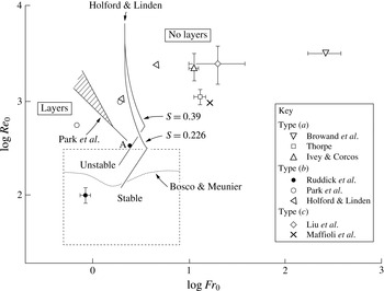
Graph of
 $\log Fr_{0}$
versus
 $\log Re_{0}$
for the various laboratory experiments of table 1. Layers are formed at relatively small values of
 $Fr_{0}$
. The stability curve of Park et al. (Reference Park, Whitehead and Gnanadeskian1994) is shown, together with their region of marginal stability (hashed). The curve is taken from their figure 3; as noted by Holford & Linden (Reference Holford and Linden1999a
) their equation for the stability boundary does not agree with the curve. Other stability curves are those derived by Holford & Linden (Reference Holford and Linden1999a
) from their experiments with
 $S=0.39$
(corresponding to their two points from the experiments referred to in table 1) and by Park et al. from experiments with
 $S=0.226$
, where
 $S=b/M$
. (The conversion from Holford & Linden’s values of Richardson and Reynolds numbers,
 $Ri$
and
 $Re$
, respectively, is
 $Fr_{0}=[(1-S)(\surd SRi)]^{-1}$
and
 $Re_{0}=Re(\surd S)/(1-S)$
. The corresponding stability curve for Ruddick et al.’s, Reference Ruddick, Mcdougall and Turner1989, experiments with
 $S=0.4$
is virtually the same as that shown for
 $S=0.39$
.) Three pairs of points from the type (b) experiments are marked; for these, layers are found at the lower values of
 $\log Fr_{0}$
and no layers at the greater values of
 $\log Fr_{0}$
. No layers appear in the Ruddick et al.’s experiments at the point marked ‘A’, which lies close to both the Park et al. and the Holford & Linden (
 $S=0.39$
) stability boundaries. The stability curve for the onset of wake instability found in the lee of a steadily moving cylinder by Bosco & Meunier (Reference Bosco and Meunier2014) is marked by a dotted line. The dashed rectangle shows the parameter range of Bosco & Meunier’s experiments.

Table 1 lists comparative values of
 $Fr_{0}$
,
 $Re_{0}$
and of
 $I_{0}$
, a measure of the characteristic turbulent buoyancy Reynolds number or isotropy index, given by
 $I_{0}=u_{0}^{3}/b{\it\nu}N^{2}$
or
 ${\it\varepsilon}/{\it\nu}N^{2}$
, where
 $u_{0}$
is the r.m.s. velocity fluctuations, determined (following Maffioli et al.
Reference Maffioli, Davidson, Dalziel and Swaminathan2014) as
 $u_{0}=0.05U$
where
 $U$
is the grid speed (or
 $a{\it\omega}$
where
 $a$
is the grid amplitude and
 ${\it\omega}$
its oscillation frequency) and
 ${\it\varepsilon}=u_{0}^{3}/b$
. The data used to derive values in table 1 are those given in or derived from tables or, when details are otherwise lacking, in the captions of figures in the respective papers. Figure 3 shows how the parameters
 $Fr_{0}$
and
 $Re_{0}$
of the various experiments vary in log space. The stability curves shown in the figure are discussed in §§ 2.2 and 4.1.
When stirring is over a limited domain or duration as in experiments of type (a) and (c), the intrusive layers are first seen to emerge at or near the outer edge of the turbulent region at a non-dimensional time,
 $(Nt)_{1}$
, of approximately 10 (table 1). The times,
 $(Nt)_{1}$
, compare to the non-dimensional time, 9.4 (a time equal to 1.5 times the buoyancy period,
 $2{\rm\pi}/N$
), for the collapse of large scales in a turbulent stratified flow in numerical studies by Staquet & Godeferd (Reference Staquet and Godeferd1998), and the non-dimensional e-folding time of 4.3 found by Smyth, Zavialov & Moum (Reference Smyth, Zavialov and Moum1997) for the collapse of turbulence following its isolation from surface forcing in the ocean. After the time,
 $(Nt)_{1}$
, layers develop as intrusions spreading into the surrounding quiescent uniformly stratified region. They are preceded by horizontally propagating internal waves. The waves advance at the group velocity appropriate to small amplitude internal gravity waves (Thorpe Reference Thorpe1982; Browand et al.
Reference Browand, Guyomar and Yoon1987; Maffioli et al.
Reference Maffioli, Davidson, Dalziel and Swaminathan2014) and are explained as being internal shear waves or columnar modes (McEwan & Baines Reference McEwan and Baines1974; Baines Reference Baines1995) generated by the intrusions. Eventually the waves reach the bounding end wall of the laboratory tank and are reflected, subsequently affecting the intrusions and the turbulent region near the grid. We return to these intrusions and internal waves in § 3.4. Only for values of
 $Nt$
of several thousand are layers first observed in experiments of type (b).
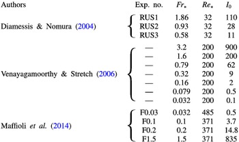
Numerical experiments simulating the collapse of turbulence in a stratified fluid. Here
 $Fr_{\ast }=u_{0}/Nl$
and
 $Re_{\ast }=u_{0}l/{\it\nu}$
and
 $I_{0}=Re_{\ast }Fr_{\ast }^{2}$
(or
 $I_{0}\sim {\it\varepsilon}/{\it\nu}N^{2}$
evaluated at time
 $t=0$
for Venayagamoorthy & Stretch’s figure 6), where
 $u_{0}$
is the r.m.s. velocity fluctuation of the initial flow,
 $l$
is the integral length scale,
 ${\it\nu}$
is the kinematic viscosity and
 ${\it\varepsilon}$
is the initial rate of dissipation of turbulent kinetic energy per unit mass. For comparison with table 1,
 $Fr_{0}\approx 20Fr_{\ast }$
and
 $Re_{0}\approx 20Re_{\ast }$
, assuming
 $u_{0}=0.05U$
following Maffioli et al. Venayagamoorthy & Stretch’s experiments are not numbered.
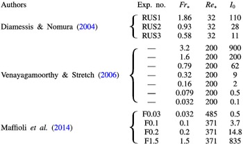
1.3 Numerical experiments
We refer in §§ 4.2 and 6 to three recent direct high resolution numerical studies (DNS) made to simulate the collapse of turbulence in a stratified fluid and which relate to the laboratory experiments. The DNS are listed in table 2 with parameter values that may be compared with values of laboratory experiments in table 1. In each DNS experiment a turbulent flow with prescribed energy spectrum, independent of stratification, is imposed initially in a uniformly stratified fluid between horizontal upper and lower boundaries. The initial buoyancy field is taken to be one in which the density fluctuations are zero and the stratification is uniform. Turbulent mixing commences at time
 $t=0$
.
Diamessis & Nomura (Reference Diamessis and Nomura2004) study homogeneous turbulence (with and without a mean shear but only the experiments without shear are addressed here) filling a horizontally bounded domain, i.e. a box. Their study with an equivalent Reynolds number,
 $Re_{0}\sim 600$
(obtained from their data by using the r.m.s. turbulent velocity,
 $u\sim 0.05U$
, following Maffioli et al.
Reference Maffioli, Davidson, Dalziel and Swaminathan2014), is aimed largely at understanding the size and three-dimensional structure of overturns in the stratified turbulent region. In their experiments with an equivalent Reynolds number,
 $Re_{0}\sim 4000$
, Venayagamoorthy & Stretch (Reference Venayagamoorthy and Stretch2006) also examine homogeneous turbulence filling a box but place more attention on the generation of internal waves and on vortices formed at
 $Nt\sim 4{\rm\pi}-150$
. Both Diamessis & Nomura and Venayagamoothy & Stretch provide estimates of the times of collapse of stratified turbulence that are useful later (in § 4.2) in the interpretation of type (b) experiments. Maffioli et al. (Reference Maffioli, Davidson, Dalziel and Swaminathan2014) study turbulence imposed initially in a rectangular region of horizontal extent smaller than the box length. The equivalent Reynolds number,
 $Re_{0}$
, is approximately 8000. A turbulent cloud is produced that spreads laterally in a way similar that of turbulence produced by the short duration oscillation of a grid in the centre of a tank in the type (c) laboratory experiment described in the same paper.
1.4 The arrangement of this paper
Possible causes of layers in the stratified turbulent flows produced by grid mixing are discussed in § 2. These include zigzag instability and the Phillips (Reference Phillips1972) and Posmentier (Reference Posmentier1977) instability (hereafter referred to as PPI). As explained in § 2.2, the field of motion in the wake of a horizontally moving grid bar is generally not homogeneous but structured, and the structure may affect the development of layers. Laboratory experiments of type (a) are described in § 3 with the main conclusions summarized in § 3.5. Type (b) experiments are addressed and compared in § 4 and an explanation for the height of layers in these experiments is proposed in § 4.4. A similarity of the intrusive layer heights in the type (a) and (c) experiments is found in § 5. The main conclusions are summarized and discussed in § 6.
2 Causes of layers
Any process that produces spatially periodic mixing in the vertical
 $z$
-direction in a uniformly stratified fluid will generate perturbations in the density field, resulting in a layered density profile with
 $z$
-periodic density gradients. In an extreme case, when processes result in very efficient mixing in the layers, the density profile will exhibit layers of uniform density separated by relatively thin, highly stratified layers. Here we consider some processes resulting from instability that may lead to such spatially periodic vertical mixing and thus multiple layers in grid mixing experiments.
A set of vertical bars moving through a stratified fluid will, in its wake, shed vortices with vertical axes. Yim & Billant (Reference Yim and Billant2015) identify and provide references to four mechanisms that may result in the instability of a single vertical vortex in a uniformly stratified fluid: shear and centrifugal instability, radiative instability (notably associated with the spontaneous radiation of internal gravity waves and observed in laboratory experiments by Riedinger, Le Dizès & Meunier (Reference Riedinger, Le Dizès and Meunier2011)) and Gent–McWilliams instability. The type of instability that may develop depends on the radial variation of vertical vorticity in the vortex. Instability may eventually lead to the formation of layers. However a moving grid will produce multiple vortices, and it is more relevant here to consider instability of more than one vortex, either through zigzag instability or the interaction of vortices in the wake of a vertical bar.
2.1 Zigzag instability of vortex pairs
Billant & Chomaz (Reference Billant and Chomaz2000) and Otheguy, Chomaz & Billant (Reference Otheguy, Chomaz and Billant2006) describe the ‘zigzag instability’ of a vertical cylindrical counter-rotating vortex pair with vertical vorticity, similar to a Lamb–Chaplygin dipole, in a uniformly stratified fluid. The dipole becomes unstable to a three-dimensional instability, periodic in the vertical direction, that ultimately leads to layers. The nonlinear evolution of the instability of the vortex pair, involving Kelvin–Helmholtz and gravitational instabilities, has been investigated numerically by Deloncle, Billant & Chomaz (Reference Deloncle, Billant and Chomaz2008), Waite & Smolarkiewicz (Reference Waite and Smolarkiewicz2008) and Augier and Billant (Reference Augier and Billant2011).
Although small-scale layers are apparent close to a vertical grid bar in the startup stages of some grid-mixing experiments (e.g. Thorpe Reference Thorpe1982, figure 8a), possibly generated by the instability of transient recirculating eddies (§ 2.2), it is not however evident how close-knit vertically coherent pairs of vortices might be produced by moving grids; streets of individual vortices are more likely, at least in type (b) experiments.
2.2 Zigzag instability in wakes
The wake of a vertical cylinder steadily moving horizontally through a uniformly stratified fluid when
 $40<Re_{0}<200$
and
 $0.3<Fr_{0}<200$
is described in experiments and a numerical model by Meunier (Reference Meunier2012). (Values of
 $U$
and
 $b$
in the definitions of
 $Re_{0}$
in (1.1) and
 $Fr_{0}$
in (1.2) are taken as the cylinder speed and diameter, respectively.) Until the onset of motions in directions parallel to the cylinder axis at
 $Re_{0}\sim 190$
, the wakes in unstratified and stratified fluids are similar. At small
 $Re_{0}$
wakes are steady; shear layers detach from the boundary layers on each side of the cylinder, producing a pair of recirculating eddies in the wake. When
 $45<Re_{0}\gtrsim 180$
, an array of vortices is produced in the cylinder’s wake, the well-known Kármán vortex street of an unstratified fluid. The vortex array consists of two rows of vortices approximately
 $2b$
apart and with vortices of one row staggered in relation to those of the other. The Strouhal number (equal to
 $b$
divided by the horizontal separation,
 $B$
, of vortices in a row) is approximately
 $0.019Re_{0}^{1/2}$
. Holford & Linden (Reference Holford and Linden1999b
) describe the wakes of square vertical bars moving horizontally through a uniformly stratified fluid when
 $1<Fr_{0}<1.83$
. The staggered double row of vortices observed in the wake of a cylinder appears for
 $40<Re_{0}<180$
but, as
 $Re_{0}$
increases, slowly develops perturbations away from the vertical. Vertical motion develops at higher
 $Re_{0}$
, wakes becoming more fully turbulent at
 $Re_{0}\sim 700$
. Holford & Linden (Reference Holford and Linden1999a
) show that even when
 $Re_{0}=1030$
vertical vortices can be identified in the wake.
Although ‘zigzag instability’ was first used to describe the instability of single vertical vortex pairs in stratified fluids, Deloncle, Billant & Chomaz (Reference Deloncle, Billant and Chomaz2011) adopt the term to describe the instability of steady vortex arrays in uniformly stratified fluids, including the vortex street shed by a horizontally moving vertical bar. Deloncle et al. examine the stability of a vortex sheet but not how it is generated by a moving grid. For a horizontal Froude number,
 $Fr_{h}\equiv |{\it\Gamma}|/(2{\rm\pi}R^{2}N)\leqslant 1$
, where
 ${\it\Gamma}$
is the circulation of the vortices of radius
 $R$
, and when the street spacing ratio,
 ${\it\kappa}$
, equal to the distance between the vortex rows divided by
 $B$
, is less than 0.41, they show that the vortex street is most unstable to a three-dimensional instability of the zigzag type that vertically bends the vortices. (As Deloncle et al. remark, the spacing ratio,
 ${\it\kappa}$
, of vortex sheets behind two-dimensional buff bodies is usually less than 0.41.) Numerical and theoretical calculations are made with Reynolds number,
 $|{\it\Gamma}|/(2{\rm\pi}{\it\nu})$
, equal to
 $5\times 10^{4}$
(corresponding to an effectively inviscid flow). The vertical wavelengths,
 ${\it\lambda}_{z}$
, of the fastest growing disturbance in a Kármán vortex street can be derived from Deloncle et al.’s figures 6 and 10. Their non-dimensional measures,
 $BFr_{h}(2{\rm\pi}/{\it\lambda}_{z})=8.5$
and 5.2 when
 ${\it\kappa}=0.2$
and 0.4, respectively, and
 $Fr_{h}=0.1$
, have corresponding
 ${\it\lambda}_{z}/b=0.37$
and 0.60, respectively, supposing that (as commonly found)
 $B\approx 5b$
, where
 $b$
is the width of the vertical bar forming the vortex street. Larger values,
 ${\it\lambda}_{z}/b=4.9$
and 8.8, are found when
 ${\it\kappa}=0.2$
, and
 $Fr_{h}=1$
and 1.2, respectively.
The estimates of
 ${\it\lambda}_{z}$
do not appear to have been verified experimentally or related to the thickness of layers observed in grid mixing experiments. Bosco & Meunier (Reference Bosco and Meunier2014) combine laboratory and numerical experiments to show that instability, and consequent layers, with a vertical wavelength of approximately
 $(4\pm 1)b$
occurs in the wake of a steadily moving vertical cylinder of diameter
 $b$
when
 $1.0<Fr_{0}<5.2$
and
 $180<Re_{0}<190$
(a range much lower than that at which Deloncle et al. estimate
 ${\it\lambda}_{z}$
). The instability is similar to the classical mode A instability in the unstratified case described by Williamson (Reference Williamson1996). Bosco & Meunier attempted to visualize the zigzag instability but it was not observed, possibly because of the limited dimensions of their laboratory tank. Turning for comparison, to the type (b) experiments: when
 $Fr_{0}=1.77$
and
 $Re_{0}=210$
, Park et al. (Reference Park, Whitehead and Gnanadeskian1994, run number 2) find layers of height
 $h\approx 5.11b$
when a single cylindrical bar moves repeatedly back and forth along the length of a tank. This estimate of
 $h$
is slightly above Bosco & Meunier’s range of
 ${\it\lambda}_{z}$
. (Park et al.’s other experiments are at greater
 $Re_{0}$
, beyond that of Bosco & Meunier.) In two experiments by Holford & Linden (Reference Holford and Linden1999a
) in which a single vertical 2.8 cm square bar moves repeatedly at constant speed through the length of a tank layers are generated with height,
 $h\approx 3.6b$
. In these experiments
 $Re_{0}=746$
and 1380 (higher than the range examined by Bosco & Meunier) and
 $Fr_{0}=1.2$
. Although this value of
 $h$
is within Bosco & Meunier’s range of vertical wavelengths, another experiment by Holford & Linden with a single square bar has the smaller height,
 $h\approx 2.3b$
when
 $Re_{0}=930,Fr_{0}=0.98$
.
In summary, because of the differing ranges of
 $Re_{0}$
, there is at best only weak evidence that the onset of zigzag instability quantified numerically by Deloncle et al. relates to that found experimentally either by Bosco & Meunier in the wake of steadily moving cylindrical bars, or to layers in the type (b) experiments with a single cylindrical bar by Park et al. or a square bar by Holford & Linden; it has not been established that the instability may be important in the generation of the layers produced by grid mixing. More experiments are needed to quantify the parameter ranges in which zigzag instability occurs and its scale and development.
2.3 The Phillips/Posmentier instability
This instability does not depend on ‘structured turbulence’, e.g. the presence of vortices in the wake of a grid, and nor does the PPI theory provide a prediction of a vertical scale of layers that it causes. A necessary condition for the occurrence of the PPI mechanism is that the vertical density flux generated by turbulence in a stratified fluid decreases as the modulus of the (negative) upward-vertical density gradient increases, a trend physically consistent with vertical motion being inhibited by increasing stratification or larger
 $|\text{d}{\it\rho}/\text{d}z|$
. An equivalent condition addressed by Holford & Linden (Reference Holford and Linden1999a
) is that the mixing efficiency, defined as the ratio of the change in the mean potential energy of the turbulent fluid to the change in available (potential and kinetic) energy, decreases as the overall (or ‘bulk’) Richardson number increases.
Layers observed in type (b) experiments (table 1 and figure 3) have sometimes been ascribed to PPI without evidence that the condition necessary for PPI is satisfied in the turbulent conditions of the experiments before layers form. Holford & Linden (Reference Holford and Linden1999a ), however, make careful measurements of the buoyancy flux and find that, even when layers subsequently develop, in the initial state the flux increases with density gradient; layers are therefore not initiated by the PPI mechanism. (An anonymous referee suggests that PPI is not detected in the initial evolution of layers because experiments have not, so far, had sufficient resolution to accurately resolve the fluxes in the initial smooth density profile.) A further important conclusion of Holford & Linden is that the flux condition necessary for the PPI mechanism is satisfied in stratified regions once the layers are formed; a layered structure is reinforced by the mechanism (see § 3.3.2). Martin & Rehmann (Reference Martin and Rehmann2006) reach the same conclusion.
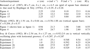
Experiments of type (a) with a continuously oscillating grid in a uniformly stratified fluid. The parameters are
 $M=$
mesh size,
 $b=$
grid bar diameter/width,
 $s=$
stroke (as used in appendix A), and
 $C$
and
 ${\it\beta}$
are non-dimensional constants defined in (3.1) and (3.2). The values of
 $a$
,
 ${\it\omega}$
,
 $N$
,
 $y$
(3.4) and
 $M/{\it\eta}$
(with
 ${\it\eta}$
given by (3.5)) are those available in figures or tables in the three publications.

2.4 Other mechanisms
There are other mechanisms, described in later sections, by which layers may be generated. Intrusions caused by the collapse of overturns in the turbulent region generated by an oscillating grid (in type (a) and (c) experiments) are discussed in §§ 3.3.1 and 3.4. Two mechanisms in type (b) experiments are further possible candidates: the distortion of vertical vortices by internal waves (§ 4.4) and mixing from the upper and lower boundaries (§ 4.5).
3 Experiments of type (a)
3.1 Local scales of turbulent motion
Three examples of the oscillating grid experiments of type (a) are listed in table 3. In the region close to an oscillating grid where, in comparison with the effects of stratification, mechanically driven turbulence is strong, motion will approximate to the unstratified turbulence generated by biplanar grids with square bars of width,
 $b$
, investigated by Hopfinger & Toly (Reference Hopfinger and Toly1976). They derive empirical expressions for the r.m.s. vertical velocity fluctuations,
 $w$
, and the integral length scale,
 $l$
:
 $$\begin{eqnarray}w=2^{1/2}C(a{\it\omega})(aM)^{1/2}/({\rm\pi}x),\end{eqnarray}$$
and
 $$\begin{eqnarray}l={\it\beta}x,\end{eqnarray}$$
at a horizontal distance,
 $x$
, from the central grid position, where
 $a$
is the amplitude of the grid motion,
 $M$
is the grid mesh length
 $-5$
or 10 cm in Hopfinger & Toly’s experiments – and
 ${\it\omega}$
is the grid frequency
 $(\text{rad}~\text{s}^{-1})$
. Values of the non-dimensional coefficients,
 $C$
and
 ${\it\beta}$
, are discussed in appendix A. The eddy time scale,
 $l/w$
, increases as
 $x^{2}$
. At some distance
 $x$
, grid-generated eddies will suffer significant collapse as a result of stratification when the eddy time scale,
 $l/w$
becomes comparable to the buoyancy time scale,
 $N^{-1}$
, i.e. when the mean local Froude number,
 $Fr=w/(Nl)$
, reaches a critical value. Using (3.1) and (3.2),
 $Fr$
can be written
 $$\begin{eqnarray}Fr=2^{1/2}Cy^{2}/({\rm\pi}{\it\beta}x^{2}),\end{eqnarray}$$
where
 $$\begin{eqnarray}y=(aM)^{1/4}(a{\it\omega}/N)^{1/2}\end{eqnarray}$$
is a length scale determined by the grid size and motion, and by the initial uniform buoyancy frequency,
 $N$
.
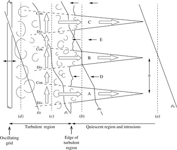
Notional sketch of the production and maintenance of intruding layers in type (a) experiments. In this vertical section, the oscillating grid is at the left and the quiescent uniformly stratified fluid to the right. Three layers emerging from the turbulent region and intruding into the quiescent fluid are drawn, A, B and C, with return flows, D and E, between A and B and between B and C, respectively. Vertical profiles of mean density are shown in the quiescent region at (a), near the edge of the turbulent region at (b), within the turbulent region at (c) and close to the oscillating grid at (d), and labelled
 ${\it\rho}_{a}$
–
 ${\it\rho}_{d}$
, respectively. The averaged scale,
 $h$
, is that commonly used to represent layer height. It may, as sketched, exceed that thickness of the regions of constant density in the intrusions emerging at the edge of the turbulent region. The length of vertical arrows at (c) indicate how the magnitude of the mean vertical flux of buoyancy varies with the density gradient, increasing the density in regions of convergence (‘con.’) and decreasing density in regions of divergence (‘div.’), and so tending to maintain the layers of small (negative) vertical density gradient in the regions feeding the intrusions and enhancing the gradients above and below these regions. The sketch differs notably from that of Browand et al. (Reference Browand, Guyomar and Yoon1987, figure 11) and reproduced by Maffioli et al. (Reference Maffioli, Davidson, Dalziel and Swaminathan2014, figure 1) in that the intruding layers are shown to begin within the turbulent region, being initially formed by the collapse of large-scale overturning eddies or ‘blobs’ that are relatively uniform in density. The vertical collapse and horizontal spreading of the blobs is asymmetrical, favouring motion away from the grid, because of the horizontal variation in Reynolds stress across their width. Internal shear waves (not drawn and of undetermined phase in relation to the intrusions; see § 6) are found to the right of the intrusions, propagating ahead of them.

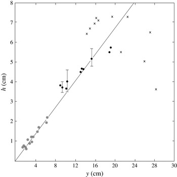
All the experiments of type (a) listed in table 3 find that
 ${\it\eta}$
, the distance of the edge of the turbulent region from the mid-position of the oscillating grid, and the thickness,
 $h$
, of intrusions measured at the edge of the turbulent region, are linearly proportional to
 $y$
, i.e.
 $$\begin{eqnarray}{\it\eta}={\it\alpha}y\end{eqnarray}$$
and
 $$\begin{eqnarray}h={\it\gamma}y,\end{eqnarray}$$
where
 ${\it\alpha}$
and
 ${\it\gamma}$
are non-dimensional coefficients that vary from one set of experiments to another. (The thickness of intrusive layers is approximately equal to the distance between neighbouring intrusions and, where several adjoining intrusions can be identified in experiments, is conveniently, easily and commonly estimated as the average distance between them. As sketched later in figure 4, however, this scale may exceed that of intrusions at the edge of the turbulent region.) The consistency found between the three experiments suggests that the Hopfinger & Toly scaling, (3.1) and (3.2), is valid for the three different grid types described in table 1, type (a) experiments. Browand et al. (Reference Browand, Guyomar and Yoon1987) find values of
 ${\it\alpha}$
and
 ${\it\gamma}$
equal to
 $1.34\pm 0.27$
and 0.34, respectively. The respective values are 0.94 and 0.34 in Thorpe’s (Reference Thorpe1982) experiments, and 1.34 and 0.32 in Ivey & Corcos’s (Reference Ivey and Corcos1982) (see Thorpe Reference Thorpe1982). Browand et al. use a vertical horizontally oscillating grid with mesh and bar size identical to one used by Hopfinger & Toly. Extrapolating from Hopfinger & Toly’s results, they adopt the values
 $C=0.29$
and
 ${\it\beta}=0.26$
. From (3.3) and (3.5), the Froude number at the edge of the turbulent region,
 $x={\it\eta}$
, can be estimated:
 $Fr=0.28$
. This is consistent with the observation by Dickey & Mellor (Reference Dickey and Mellor1980) that the character of motion in the wake of a horizontal grid moving vertically upwards in a uniformly stratified fluid changes from turbulence to internal waves where
 $Fr=0.27$
. Using (3.2), (3.5) and (3.6), at the boundary of the turbulent region,
 $h/l={\it\gamma}/{\it\beta}{\it\alpha}=1.01\pm 0.20$
, or
 $h\approx l$
at
 $x={\it\eta}$
as speculated by Thorpe (Reference Thorpe1982). Values of
 $C$
and
 ${\it\beta}$
are unknown for the grids used by Thorpe and Ivey & Corcos but can be inferred as
 $C=0.204$
, 0.267 and
 ${\it\beta}=0.37$
, 0.247, respectively by making the similarity assumption that
 $Fr=0.28$
and
 $h=l$
at
 $x={\it\eta}$
.
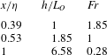
Values obtained from Browand et al.’s (Reference Browand, Guyomar and Yoon1987) type (a) experiments using
 $C=0.29$
,
 ${\it\beta}=0.26$
,
 ${\it\alpha}=1.34$
,
 ${\it\gamma}=0.34$
and listed in order of increasing
 $x/{\it\eta}$
through the turbulent region. (
 $x/{\it\eta}=1$
is the location of its mean boundary.
 $h/L_{O}$
increases with
 $x/{\it\eta}$
.)

The local Ozmidov length scale,
 $L_{O}={\it\varepsilon}^{1/2}/N^{3/2}$
, equals
 $$\begin{eqnarray}L_{O}=2^{3/4}C^{3/2}y^{3}/({\rm\pi}^{3/2}x^{2}{\it\beta}^{1/2}),\end{eqnarray}$$
taking the rate of dissipation of turbulent kinetic energy per unit mass,
 ${\it\varepsilon}$
, as
 $w^{3}/l$
. Using (3.3)–(3.6), corresponding values of
 $x/{\it\eta}$
,
 $h/L_{O}$
and
 $Fr$
from Browand et al.’s experiments are found and specified in table 4. The ratio
 $h/L_{O}$
exceeds 1 at
 $Fr=1$
and, as shown by (3.3),
 $Fr$
decreases as
 $x/{\it\eta}$
increases through the turbulent region. At the edge of the turbulent region,
 $h$
(and therefore
 $l$
), is much greater than the scale of the largest overturning eddies,
 $L_{O}$
, so that the turbulent motion is largely horizontal.
As conjectured by Maffioli et al. (Reference Maffioli, Davidson, Dalziel and Swaminathan2014) the local Froude number, Fr, provides values that determine the character of the turbulent flow. Further evidence that a Froude number characterises the state of the stratified turbulent motion is provided by the stability curves in figure 3: layers form only when
 $Fr_{0}$
is less than a value of approximately unity. As outlined in appendix B, the local buoyancy Reynolds number,
 $I$
, does not provide such a similarity parameter. Moreover, the local Reynolds number,
 $Re=wl/{\it\nu}$
, is independent of
 $x$
and therefore also cannot be an effective parameter to define the local state of turbulence.
In summary, the size,
 $h$
, of layers in the type (a) experiments is given by
 $h={\it\gamma}y$
, with
 ${\it\gamma}=0.33\pm 0.01$
. The bar scales of the three experiments listed in table 1,
 $b=1.0~\text{cm}$
, 0.64 cm and 1.27 cm, respectively, do not appear to provide the size or scaling of the layer thickness,
 $h$
, that might be expected if the layers result from zigzag instability of a vortex street (e.g.
 $h\approx 4b$
; § 2.2). Indeed how the instability of a vortex pair or vortex street might apply to the disorganized mêlée of vortices shed by a rapidly oscillating grid is not obvious.
3.2 The origin of layers
3.2.1 Collapsing overturns
Browand et al. (Reference Browand, Guyomar and Yoon1987) note that although intrusive layers are not visible until they reach the edge of the near-grid turbulent region, the turbulence itself is affected by the layering at times of
 $(2{-}3)Nt$
, before the intrusions emerge and become apparent at
 $Nt=9.6\pm 2.5$
(table 1). They also remark that ‘an effective origin in time’ for the advance of intrusive layers is ‘much nearer to the onset of grid motion’ than to some other, more arbitrary, initial time. Similarly, Thorpe (Reference Thorpe1982) finds that the horizontal extent of layers is proportional to
 $y(Nt)^{p}$
, where
 $t$
is the time elapsed from the start of grid oscillation and
 $p$
is a constant near 0.4; layers appear to be first formed near the oscillating grid and at a time close to that at which grid stirring begins.
We shall suppose that initially ‘blob-like’ roughly spherical overturns with height of order
 $L_{O}$
are produced within the turbulent region, and that the blobs collapse and spread to supply fluid that initially forms the intrusions. Whilst noting the uncertainty in characterising the intrusion height by the measured scale,
 $h$
, and an overturn by
 $L_{O}$
, if volume is (approximately) conserved the height of an overturn leading to an intrusion must equal or exceed that of the intrusion unless the fluid of the overturn is supplemented during its collapse.
3.2.2 The size of overturns
It is evident from table 4 that only close to the grid, at
 $x/{\it\eta}<0.39$
, does the Ozmodov scale,
 $L_{O}$
, exceed
 $h$
. There are reports, however, of layers of thickness exceeding
 $L_{O}$
in laboratory experiments. Browand et al. (Reference Browand, Guyomar and Yoon1987) noticed layers with a vertical scale ‘approximately 7 times the estimated Ozmidov scale at
 $Nt=10$
’, the time,
 $t$
, being that when the front of the turbulent region surrounding the grid begins to break up with the formation of layers. This estimate is in accord with the value
 $h/L_{O}$
at
 $x/{\it\eta}=1$
in table 4. In experiments of type (b) with continuous stirring throughout the tank, Ruddick et al. (Reference Ruddick, Mcdougall and Turner1989) find that ‘the observed layer thicknesses were always larger than the Ozmidov scale’. They estimate
 $L_{O}$
as
 $(5K_{{\it\rho}}N^{-1})^{1/2}$
where
 $K_{{\it\rho}}$
is the molecular diffusivity of density (rather than an eddy diffusivity that might be more appropriate). This gives
 $L_{O}=(0.2{-}0.3)~\text{mm}$
or less, smaller than the layers which are typically 2 cm in height. The smallest layers observed are of scale 0.6 cm after 150 min of grid stirring. In one experiment they do however report: ‘irregular variations in the density gradient of scale 1–2 cm were apparent…. together with finer-scale striations of approximately 1 mm spacing’. The greater-than-
 $L_{O}$
thickness of layers may be because of layer merging leading, in the long-duration experiments of type (b), to thicker layers. Indeed Ruddick et al. comment that, in one experiment, ‘the thicker layers may have formed by the merging of thinner layers’. Although recognised as a potentially significant process by Browand et al. (Reference Browand, Guyomar and Yoon1987), Liu et al. (Reference Liu, Maxworthy and Spedding1987), Balmforth, Llewellyn Smith & Young (Reference Balmforth, Llewellyn Smith and Young1998) and Wunsch & Kerstein (Reference Wunsch and Kerstein2001), there appears to be insufficient quantitative information to determine the general importance of layer merging in establishing the height of intrusions. All the type (b) experiments show that layers can exist and survive within a turbulent, actively stirred region through which a grid is moving.
An r.m.s. displacement (or Thorpe) scale,
 $L_{T}$
, is often used to characterise the vertical scale of density overturns. From observations in a freshwater lake and at sea Dillon (Reference Dillon1982) suggests
 $L_{O}/L_{T}\sim 0.8$
while Peters, Gregg & Toole (Reference Peters, Gregg and Toole1988) and Ferron et al. (Reference Ferron, Mercier, Speer, Gargett and Polzin1998) conclude
 $L_{O}/L_{T}\sim 0.95$
; both relations imply that the r.m.s. displacement scale,
 $L_{T}$
, exceeds
 $L_{O}$
. In numerical experiments on collapsing stratified turbulence, however, Mater, Schaad & Venayagamoorthy (Reference Mater, Schaad and Venayagamoorthy2013) find the ratio,
 $L_{T}/L_{O}$
, increases as the characteristic Froude number,
 $Fr$
, decreases, with
 $L_{T}\sim L_{O}$
where
 $Fr=1$
. If the numerical results can be used as a guide, they imply that
 $L_{T}>L_{O}$
in the outer part of the turbulent region surrounding the oscillating grid. The scale
 $L_{T}$
is, however, observed to be distributed log normally (Stansfield, Garrett & Dewey Reference Stansfield, Garrett and Dewey2001) with some individual values much greater than the mean. Itsweire (Reference Itsweire1984) finds that the maximum size of overturns,
 $L_{max}$
, is 2.74 times the r.m.s.,
 $L_{T}$
, a scaling supported by measurements in grid-generated turbulence by De Silva & Fernando (Reference De Silva and Fernando1998). Taking
 $L_{T}=(1/0.8)L_{O}$
in accord with Dillon’s results, and
 $L_{max}=2.74L_{T}$
, gives
 $L_{max}\approx 3.4L_{O}$
. Since (from (3.7))
 $L_{O}\propto x^{-2}$
and
 $L_{O}/h=1$
at
 $x/{\it\eta}=0.39$
(table 4),
 $L_{max}/h\approx 3.4$
at
 $x/{\it\eta}=0.39$
and
 $L_{max}/h\approx 1$
at
 $x/{\it\eta}=0.72$
. It follows that within the turbulent region near
 $x/{\it\eta}\sim 0.4$
, overturns occur of height,
 $L_{max}$
, substantially exceeding
 $h$
.
Similar layers can be seen at the same vertical location on the two sides of the grid oscillating in mid-tank shown in figure 2(d–g). This implies that layers have a common origin near the grid and, at least for the grid in the figure with solidarity parameter,
 $S=0.34$
, a structure that survives the stirring motion of the grid (as in the type (b) experiments) by transmitting information through it, perhaps initially by fluid transfer but more likely, in later stages, by pressure gradients.
3.3 Sustaining layers within the turbulent region
3.3.1 Spread of large overturns
Apart from the conclusions reached in § 3.2, there is little information provided by the laboratory experiments about the processes within the turbulent region that lead to the generation and maintenance of intrusions. The intruding fluid moving from the turbulent region must be replaced by ambient fluid in a return flow into the turbulent zone as sketched in figure 4 or, for example, in Browand et al.’s (Reference Browand, Guyomar and Yoon1987) figure 11. Figure 4 shows three intruding layers, A, B and C. Density profiles are shown at four horizontal locations, (a–d). The vertical density gradient in the return flows, D and E, between intrusions, is modified as the return flow narrows as it approaches and enters the turbulent region, tending to strengthen the density gradients above and below the spreading fluid and inducing within the turbulent region a variation in the vertical density gradient. Browand et al. imagine a process of self-regulation in which, if an intrusion slows down, so does the return flow. Consequently the grid, deprived of this stratified return flow, is able to mix the fluid more thoroughly, supplying the intrusion with more well-mixed fluid, resulting in an increase in its speed. The converse applies: if an intrusion speeds up, so does the return flow resulting in a less well-mixed supply and a subsequent decrease in the speed of the intrusion. This control process does not however lead to an estimate for
 $h$
.
A further feature in the spreading of relatively mixed layers within the turbulent layer is the horizontal variation of Reynolds stress,
 $\langle {\it\rho}uw\rangle$
. Layers span a region of rapidly decreasing Reynolds stress (
 $\langle {\it\rho}uw\rangle \propto x^{-2}$
through (3.1) since the fluctuations in the vertical and horizontal velocity fluctuations,
 $w$
and
 $u$
, are of similar magnitude near the grid). The eddy stresses on the grid side of a relatively well-mixed blob will impede its collapse under gravity (driven by the horizontal pressure gradients resulting from the differences in density within and outside the blob) more than do the stresses of smaller weaker eddies on the side of a blob furthest from the grid. A spread of a blob away from the grid is therefore favoured, and this must help induce the return flow.
3.3.2 A Phillips/Posmentier process
Although PPI does not appear to initiate layers (§ 2.3), the instability mechanism may help sustain layers once they are formed (Holford & Linden Reference Holford and Linden1999a ). Assuming that Holford & Linden’s finding that PPI can occur in turbulent but layered conditions and that those in their type (b) experiments are similar to those near the oscillating grid in the type (a) experiments, the turbulent flux of density will decrease as the negative vertical density gradient increases. There is therefore a decrease in the upward-vertical buoyancy flux where the negative density gradient is large, i.e. within the layers above and below the intrusion at section (c) in figure 4, and an increase in the upward buoyancy flux where the negative density gradient is small, i.e. within the fluid of the intrusion. These variations in flux are indicated by the vertical arrows in figure 4. Just as in Phillips’ instability theory the result is that the density near the base of the intrusion is decreased and that near the top is increased; differences in density across the layers above and below the intrusion are increased. The region of relatively mixed fluid originally in an overturn is enhanced and sustained within the turbulent region, and so too are the pressure gradients that lead to its spreading.
3.4 The speed of intrusions and internal waves
3.4.1 Internal shear waves
The greatest speed at which internal waves generated by the grid turbulence can radiate horizontally corresponds to that of internal shear waves or columnar modes and is given by the horizontal component of the group velocity,
 $c_{gx}=N/m$
, where
 $m$
is their vertical wavenumber (putting
 $k=0$
in (C 2) in appendix C). Vertical dye lines in the stratified ambient water ahead of the intrusions in the experiments by Thorpe (Reference Thorpe1982) and Browand et al. (Reference Browand, Guyomar and Yoon1987) show the early arrival of oscillations with vertical wavelengths,
 ${\it\lambda}_{z}\,(=2{\rm\pi}/m)$
, roughly twice the vertical distance between the intrusions at a time consistent with the propagation speed
 $c_{gx}$
. There are two shear layers produced by the shear waves, one of positive horizontal vorticity and one negative, in each internal wave vertical wavelength, a point to which we return in §§ 4.4 and 6. Maffioli et al. (Reference Maffioli, Davidson, Dalziel and Swaminathan2014, and private communication with Dr A. Maffioli, October ’14) find that the vertical wavelength of the horizontally travelling internal waves, judged from twice the distance between pearlessence-revealed shear layers in their laboratory experiments, is approximately twice that of the intrusions. This is consistent with the findings of Browand et al. and Thorpe. In § 3.4.4 we address the question of why a scale of approximately
 $2h$
is favoured.
3.4.2 The speed of waves and intrusions in other studies
The speed at which internal waves and intrusions spread in a uniformly stratified fluid of buoyancy frequency,
 $N$
, is discussed by Bolster, Hang & Linden (Reference Bolster, Hang and Linden2008) and by Maurier & Linden (Reference Maurier and Linden2014). In their ‘lock-break’ laboratory and numerical experiments the latter show that intrusions spread at uniform speeds after a short initial stage of acceleration and until intrusions are affected by the reflection of internal waves from the end of the tank. An ‘intermediate intrusion’ of fluid with density equal to the mean of those at the upper and lower horizontal boundaries spreads at half-tank depth with a speed of approximately half that of density currents spreading along the upper or lower boundaries. These boundary density currents are found by Maxworthy et al. (Reference Maxworthy, Leilich, Simpson and Meiburg2002) and by Bolster et al. to advance at speeds of approximately
 $0.25NH$
, where
 $H$
is the tank depth. Maurier & Linden show that the speed of intermediate intrusions is explained by noting that they are equivalent to two boundary density currents, one above a surface dividing the intrusion into two at the half depth, the other below. Since each of these is in an effective depth of
 $H/2$
, their speeds are
 $0.25N(H/2)=0.125NH$
.
Gravity currents with density greater or less than that in the ambient uniformly stratified fluid, namely those spreading along the lower or upper boundaries, respectively, generate internal waves. Long internal shear waves of mode 1 advance ahead of them; the long-wave group velocity
 $c_{g}=NH/{\rm\pi}$
exceeds the gravity current speed,
 $0.25NH$
. The speed of long mode 2 internal shear waves,
 $NH/2{\rm\pi}$
, is, however, less than that of these density currents and so mode 2 waves cannot propagate ahead of them. Similarly intrusions of intermediate density spreading into uniformly stratified fluid at height less than
 $0.27H$
or greater than
 $0.73H$
above the bottom travel at speeds less than the mode 1 internal waves but greater than the second mode waves (Bolster et al.
Reference Bolster, Hang and Linden2008). However, intrusions spreading at heights between
 $0.27H$
and
 $0.73H$
, for example those with the mean density, which travel at mid-depth, produce long mode 2 waves (by symmetry) that advance at speed
 $NH/2{\rm\pi}$
. These are in excess of the speed of the intrusion and are able to propagate ahead of it.
3.4.3 Boundary density currents generated by grid mixing
Because there is no vertical density flux through the horizontal boundaries at the top and bottom of the tank, mixing by the grid forms layers of relatively uniform density, that at the upper boundary being of density slightly greater than that in the ambient fluid at the top of the tank. Similarly the mixed layer at the lower boundary is slightly less dense than that in the ambient at the bottom. These layers intrude horizontally as density currents into the ambient fluid close to the respective horizontal boundaries (e.g. as is visible near the upper boundary in figure 2), and will generate long internal waves mainly of mode 1 which travel at a speed
 $NH/{\rm\pi}$
. It is shown in appendix C that these appear unlikely to affect the intrusions emerging in the experiments from the turbulent region at times,
 $Nt$
, less than 16, with the possible exception of those intrusions that neighbour these boundary currents.
3.4.4 The speed of the intrusions in the grid mixing experiments
Thorpe (Reference Thorpe1982) and Browand et al. (Reference Browand, Guyomar and Yoon1987) find that the mean non-dimensional speed of intrusions, d
 $l_{i}$
/d
 $t$
, is approximately given by
 $$\begin{eqnarray}(1/Nh)\text{d}l_{i}/\text{d}t={\it\chi}(Nt)^{-q},\end{eqnarray}$$
where
 $l_{i}$
is the length of an intrusion and
 $h$
is the intrusion height. In Browand et al.’s experiments the non-dimensional coefficient
 ${\it\chi}$
varies from approximately 0.49 to 1.0 as the exponent,
 $q$
, varies from 0.3 to 0.5 when
 $Nt$
exceeds a value of approximately 4 and before internal waves reflect from the end of the tank. In Thorpe’s experiments
 ${\it\chi}\sim 0.69$
and
 $q\sim 0.56$
when
 $2\leqslant Nt\leqslant 20$
. These values give intrusion speeds,
 $\text{d}l_{i}/\text{d}t$
, ranging from
 $0.25Nh$
to
 $0.32Nh$
in Browand et al.’s experiments and equal to
 $0.19Nh$
in Thorpe’s, at the non-dimensional time,
 $(Nt)_{1}\approx 10$
(table 1), when intrusions are observed to emerge from the turbulent region. (Greater speeds are observed at smaller
 $Nt$
.) These speeds exceed Maurier & Linden’s estimate,
 $0.125Nh$
, of the speed of intermediate intrusions confined between levels separated in the vertical by
 $h$
(§ 3.4.2). They are indicative of different forcing processes. Unlike the constant speed intrusions formed by lock-breaking and continually supplied by fluid from behind the ‘lock’, or sustained by mixing from the mean level of a vertically oscillating horizontal grid (De Silva & Fernando Reference De Silva and Fernando1998), the type (a) intrusions continually decelerate (as in (3.8)). This is consistent with their formation being transient and not sustained as in the ‘lock-break’ scenario.
The initial speeds of advance of intrusions from the turbulent region, ranging from
 $0.19Nh$
to
 $0.32Nh$
, exceed the horizontal group velocity,
 $c_{gx}=N/m=Nh/2{\rm\pi}\approx 0.16Nh$
, of internal shear waves with vertical wavelength,
 $h$
, which therefore cannot propagate ahead of the intrusions. The advance of a vertical array of intrusions separated by a vertical length,
 $h$
, will however generate a spectrum of internal waves. It is shown in appendix D that only waves with vertical scale equal to or exceeding
 $2h$
can propagate ahead of the intrusions. This is in accordance with the observed wavelengths,
 ${\it\lambda}_{z}\sim 2h$
(§ 3.4.1). Because intrusion speeds decrease with
 $Nt$
, however, waves of vertical scale
 $h$
are able to advance faster than the intrusions when
 $Nt$
is sufficiently large. Like the intrusions themselves, the scale of the waves dominant at large times must be related to the presently unknown spatial and temporal distribution of collapsing mixed regions within the turbulent region.
3.5 Summary of §§ 3.1–3.4
It is yet to be shown whether zigzag instability can generate the layers observed in the type (a) experiments (§ 3.1), but it appears unlikely except perhaps as a grid of vertical bars is first set into motion (§ 2.1). Holford & Linden (Reference Holford and Linden1999a
) find that the PPI mechanism may help sustain, but not cause, layers in the turbulent region. The local Froude number,
 $Fr$
, characterises the variation of the state of turbulence with distance from its generation by the moving grid. The height of overturns,
 $L_{max}$
, well within the turbulent layer (e.g. at
 $x/{\it\eta}\sim 0.4$
) substantially exceeds the layer height,
 $h$
(§ 3.2.2). Overturns are consequently sufficiently large to produce intruding layers of the height,
 $h$
, observed at the edge of the turbulent region. In § 3.2.1 it is shown that the variation in time of the intrusions’ horizontal extent is consistent with their starting at about the time when the grid is first set in motion. There is a similarity of layers on the two sides of a grid oscillating in the centre of a tank (§ 3.2.2). These conclusions imply that layers in continuously forced, type (a) (and possibly transiently forced, type (c)) experiments are formed soon after the grid stirring begins and may have connection through an oscillating grid.
In § 3.4 it is found that the leading internal waves propagating ahead of the intrusions have a vertical wavelength of approximately
 $2h$
, twice the thickness of the layers; waves of smaller vertical scale do not travel fast enough to advance more rapidly than the intrusions when they are first observed, emerging from the turbulent region. The sometimes remarkable vertical periodicity and regularity of intrusions remains unexplained.
4 Experiments of type (b)
4.1 Stability curves
Three experiments of type (b) in which the whole tank is stirred are listed in table 1. Layers are not observed until after stirring has continued for times exceeding some thousands of buoyancy periods. The stability curve determined empirically by Park et al. (Reference Park, Whitehead and Gnanadeskian1994) is shown in figure 3, together with a neighbouring (hatched) region in which they report that it is uncertain whether layers are formed or not. The stability curve separates two regimes recognised in their experiments: a regime of sufficiently low
 $Re_{0}$
and low
 $Fr_{0}$
in which layers are observed and a regime at higher
 $Re_{0}$
and
 $Fr_{0}$
in which no layers appear. Parameter values of two of Park et al.’s experiments, one in each regime, are given in table 1 and shown as circles in figure 3. The experiments in which layers are observed by Ruddick et al. (Reference Ruddick, Mcdougall and Turner1989) lie within Park et al.’s layer regime even though the apparatus and experimental details differ (e.g. Park et al. have one stirring rod, Ruddick et al. have many). Ruddick et al.’s experiment in which no layers form (point marked as ‘A’ in figure 3) lies very close to the (imprecise) position of the stability curve, consistent with the expectation from Park et al.’s study that the turbulent flows are at best weakly unstable.
As mentioned in § 2.3, Holford & Linden (Reference Holford and Linden1999a
) find that PPI is not a cause of layers. Rather they conclude that vertical mixing resulting from bending of vertical vortices shed by the moving grid bars causes the layers. Their explanation does not, however, account for the height of observed layers. They establish an empirical stability curve dividing the regions in which layers are formed from that in which they are absent. The curve depends on the grid scale parameter
 $S$
. Two of the curves are shown in figure 3. These correspond to the value
 $S=0.39$
in Holford & Linden’s experiments referred to in table 1 and shown as points in figure 3, and to
 $S=0.226$
corresponding to Park et al.’s experiments (although there, with only one stirring bar, the mesh size,
 $M$
, is uncertain. It is somewhat arbitrarily taken as the tank width. This may account for the difference between the Park et al.’s stability curve and Holford & Linden’s curve
 $S=0.226$
).
4.2 The effect of turbulence ahead of the grid
Ambient turbulence in the tank, encountered and supplemented by the stirring grid after its first cycle, may affect the formation of vortices in the grid wake which are found by Holford & Linden to be necessary for the generation of layers. Turbulence produced by the moving grid decays in time. The repetition period of stirring by the cycling grid depends on position along the length of the tank. At the centre this period is
 $L_{s}/U$
, where
 $L_{s}$
is the horizontal length of grid motion, and at the ends of the grid stroke it is
 $2L_{s}/U$
. The r.m.s. time period is
 $T_{\ast }=\surd (8/3)(L_{s}/U)$
. (This is found by integrating and summing the squares of
 $X$
and
 $(1-X)$
, where
 $XL_{s}$
is the distance along the tank from the end of a grid stroke, then taking the square root.)
 $NT_{\ast }$
characterises the non-dimensional mean time between grid stirring events. Suppose that the processes producing layers as the grid passes by (e.g. those to be described in § 4.4) are only effective if the turbulence left by previous cycles of the grid has decayed sufficiently. Marginal conditions for layer generation exist when the time,
 $T_{d}$
, for turbulence to collapse is equal to
 $T_{\ast }$
, i.e. when
 $$\begin{eqnarray}NT_{d}=\surd (8/3)(NL_{s}/U),=\surd (8/3)(L_{s}/b)Fr_{0}^{-1}.\end{eqnarray}$$
If the non-dimensional time for the decay of turbulence in a stratified fluid is known as a function of
 $Re_{0}$
this equation defines the stability boundary separating conditions in which layers can or cannot be formed. Values of
 $NT_{d}$
smaller than
 $\surd (8/3)(L_{s}/b)Fr_{0}^{-1}$
imply conditions in which turbulence has decayed substantially between grid strokes so that the processes leading to layers can operate, unaffected by the residual turbulence. Alternatively, given the relation between
 $Re_{0}$
and
 $Fr_{0}$
defined by the stability curves of figure 3 and values of
 $L_{s}/b$
in the related experiments, (4.1) can be used to determine the value of
 $NT_{d}$
as a function of
 $Re_{0}$
for which marginal conditions are found.


Points at various values of
 $Re_{0}$
(with corresponding values of
 $Fr_{0}$
) on the stability curves of Park et al. (Reference Park, Whitehead and Gnanadeskian1994) and Holford & Linden (Reference Holford and Linden1999a
) shown in figure 3 are selected. Table 5 gives values of the non-dimensional turbulence collapse time,
 $NT_{d}$
, determined using (4.1) for which conditions are marginal and turbulence does not affect the process of layer formation. These values increase with
 $Re_{0}$
. They span the times
 $(Nt)_{1}\sim 10$
for the emergence of layers from the turbulent region in type (a) experiments, and those of numerical experiments mentioned in § 1.3 and listed in table 3. In the latter
 $Nt\sim 2{\rm\pi}$
and 10 are found by Venayagamoorthy & Stretch (Reference Venayagamoorthy and Stretch2006) and by Maffioli et al. (Reference Maffioli, Davidson, Dalziel and Swaminathan2014, and private communication with Dr A. Maffioli, June, 2015) to characterise the cessation of overturning and the suppression of turbulent mixing when
 $Re_{0}\sim 4000$
and 8000, respectively. Diamessis & Nomura (Reference Diamessis and Nomura2004) find
 $Nt=4.5$
when the volume fraction of overturns tends to zero, when
 $Re_{0}\sim 600$
.
These times imply that in the type (b) experiments the production of overturning eddies by the turbulence virtually ceases between successive mixing by grids in those type (b) experiments listed in table 1 in which layers are formed. For example, selecting two type (b) experiments listed in table 1 where stirring produces layers, the time
 $\surd (8/3)(L_{s}/b)Fr_{0}^{-1}$
is 14.6 in Park et al.’s figure 8 at
 $Re_{0}=548$
, and 16.8 in Holford & Linden’s figure 6 at
 $Re_{0}=1100$
. Both exceed values of the non-dimensional turbulent decay times,
 $NT_{d}$
, in table 5. In these experiments, on average the grids advance into relatively weak residual turbulence left from their last cycle. Coherent vortices (§ 2.2) shed by the grid may then survive in the turbulent motion left from earlier grid stirring. In contrast, layers are not observed in conditions in which a vortex wake may be suppressed by turbulence still active from earlier grid stirring.
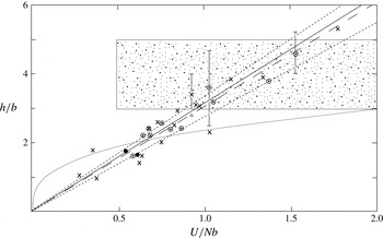
The variation of
 $h/b$
with
 $U/Nb\,(=Fr_{0})$
for type (b) experiments. Points (●) are from Ruddick et al. (Reference Ruddick, Mcdougall and Turner1989), crosses (
 $\times$
) are from Park et al. (Reference Park, Whitehead and Gnanadeskian1994) and open circles (○) are from Holford & Linden (Reference Holford and Linden1999a
). The fitted long dashed line is
 $h/b=3.03U/Nb$
, and the short dashed lines,
 $(3.03\pm 0.3)U/Nb$
, (4.4), indicate its possible uncertainty. The full line is the relation (4.6) derived in § 4.4 in which vortices shed by the grid bars are supposed to be bent by internal waves moving with the grid at speed
 $U$
. The dotted curve is the best fit, (5.1), determined by Maffioli et al. (Reference Maffioli, Davidson, Dalziel and Swaminathan2014) from their laboratory experiments of type (c), although these are in the range
 $16<U/Nb<74$
, beyond that of the type (b) experiments (see figure 6). The stippled region indicates the range of
 $h/b$
observed by Bosco & Meunier (Reference Bosco and Meunier2014).

4.3 The layer height
Layer heights in type (b) experiments are found to be related to
 $U/N$
. Park et al. (Reference Park, Whitehead and Gnanadeskian1994), stirring with single vertical cylindrical bars of diameter,
 $b=1.29$
, 2.26 and 3.37 cm, find
 $$\begin{eqnarray}h~(\text{cm})=2.6U/N+1~\text{cm},\end{eqnarray}$$
independent of
 $b$
, with
 $h$
,
 $U$
and
 $N$
in cgs units, over a range of
 $U/N$
from approximately 0.5 to 3 cm. Holford & Linden (Reference Holford and Linden1999a
) use a variety of grids composed of 1–8 square vertical bars,
 $b$
ranging from 0.65 to 3.15 cm. They conclude
 $$\begin{eqnarray}h=3.07U/N,\end{eqnarray}$$
again independent of
 $b$
, in the range of
 $U/N$
from approximately 0.7 to 4.2 cm. (As mentioned in § 1.2, Ruddick et al. (Reference Ruddick, Mcdougall and Turner1989) have a complex stirring device with cylindrical bars of diameter 1.2 cm. Given values of
 $h~(\text{cm})$
are
 $2.72U/N$
for
 $U/N=0.73~\text{cm}$
and
 $3.27U/N$
for
 $U/N=0.64~\text{cm}$
, fairly close to and bracketing values in (4.3). Here
 $U$
is taken as
 $a{\it\omega}/\surd 2$
where
 ${\it\omega}$
is the grid frequency and
 $a$
is the amplitude of the grid motion.) Figure 5 is a graph showing the variation of
 $h/b$
with
 $U/Nb$
for the type (b) experiments. There is general alignment of points between the lines
 $$\begin{eqnarray}h/b=(3.03\pm 0.3)U/Nb\end{eqnarray}$$
(or
 $h/b=(3.03\pm 0.3)Fr_{0}$
).
The vertical scale of the instability in the wake of a horizontally moving vertical cylinder found by Bosco & Meunier (Reference Bosco and Meunier2014) to be
 $(4\pm 1)b$
, independent of Froude number, is shown by the stippled region of figure 5. It is inconsistent with the type (b) experiments. As shown in figure 3, however, Bosco & Meunier’s study is at lower Reynolds number than that of the type (b) experiments. Further study is merited.
4.4 Internal waves and vortices
Although internal waves are not reported in the long-running experiments of type (b), it is probable that they are generated, particularly in the relatively low forcing conditions (larger
 $NT_{d}$
) when layers are observed and the turbulence in the fluid into which the grid moves is relatively weak. Suppose that the motion of the grid through the tank at speed
 $U$
generates horizontally travelling internal waves. The optimally generated waves are those with group speed,
 $c_{gx}=N/m$
(and, as shown in appendix C, an equal phase speed), that match (and remain in phase with) the grid:
 $c_{gx}=U$
, where
 $m=2{\rm\pi}/{\it\lambda}_{z}$
is the vertical wavenumber and
 ${\it\lambda}_{z}$
is the vertical wavelength of the waves. The latter is therefore given by
 $$\begin{eqnarray}{\it\lambda}_{z}=2{\rm\pi}U/N,\end{eqnarray}$$
provided that vertical wavelengths of appropriate scale are excited. Using the relation between
 $U/Nb$
and
 $h/b$
(4.4) of figure 5 it follows that
 ${\it\lambda}_{z}=(2.07\pm 0.21)h$
; internal shear waves that propagate with the speed of the grid have a vertical wavelength of approximately twice the observed layer height.
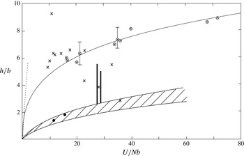
The variation of
 $h/b$
with
 $U/Nb\,(=Fr_{0})$
for (i): the type (a) experiments by Thorpe (Reference Thorpe1982) indicated by the hatched range, including the two referred to in table 3 shown by ●, and Browand et al. (Reference Browand, Guyomar and Yoon1987), marked by bold range bars (with an off-scale point at
 $h/b=8.7,U/Nb=180$
omitted); (ii) the type (b) experiments (indicated by the dashed line at relatively small
 $U/Nb$
and shown in greater detail in figure 5); and (iii) type (c) experiments, where the circles (○) are points from Maffioli et al.’s (Reference Maffioli, Davidson, Dalziel and Swaminathan2014) experiments fitted by the long-dashed line, (5.1), and where the vertical bars indicate uncertainty, and the crosses (
 $\times$
) are from the experiments by Liu et al. (Reference Liu, Maxworthy and Spedding1987) (see appendix E).

Holford & Linden (Reference Holford and Linden1999b
) describe the development of vertical vortices in the lee of eight vertical bars with
 $b=0.65~\text{cm}$
in type (b) experiments. They observe that in experiments with
 $Re_{0}<140$
and, approximately
 $1.0<Fr_{0}<1.9$
, the vortices are bent in the
 $x$
-direction of the grid motion, becoming sinusoidal in the vertical. The effect of bending the vertical vortices is to produce a horizontal component of vorticity in the
 $x$
-direction, the maximum (positive) and minimum (negative) horizontal components of
 $x$
-vorticity in each vertical wavelength both tending to overturn isopycnals. This leads to layers with a vertical height half that of the bent vortices.
The possible existence and effect of shear waves is not recognised by Holford & Linden. The agreement of scales of layers and waves supports the conclusion that the mechanism causing the layers is an interaction of the vertical vortices and the internal shear waves generated by the moving vertical grid bars. As noted in § 3.4.1, the internal waves generate two shear layers in each vertical wavelength, one of positive horizontal vorticity and one negative. Bending the vertical vortices, these shear layers result in mixed layers of height
 $h={\it\lambda}_{z}/2$
or, from (4.5),
 $$\begin{eqnarray}h/b={\rm\pi}Fr_{0},\end{eqnarray}$$
implying a value of
 $h/b$
well within the scatter of observed points in figure 5.
What happens when the grid bars reverse their horizontal motion at the two ends of the tank? The conditions at the upper and lower ends of the bars determine the phase of waves and the location of associated shear layers along the vertical bars. The phase can adjust by half a vertical wavelength when the direction of bar motion reverses; the particle motions within the shear layers composing the waves continue to be forced even though the direction of grid motion and wave propagation is reversed at the end of each grid stroke. Since layers are formed by mixing at the levels where the internal wave shear is a positive or negative maximum, the mean horizontal flow induced there by the internal waves is zero; the vertical phase of the horizontal flow induced by the waves is
 ${\rm\pi}/2$
out of phase with that of the shear. It is therefore not expected that the layers will be in relative motion. (No examination of the relative mean flow in the layers appears to have yet been made to confirm or refute this conclusion.)
The long times,
 $(Nt)_{1}$
, required for the formation of layers in the type (b) experiments (table 1) are presumably a consequence of the relatively weak forcing of internal waves by the grids. The effect of molecular viscosity,
 ${\it\nu}$
, and diffusivity,
 ${\it\kappa}$
, on the internal shear waves is very small, tending slightly reduce their horizontal phase speed and to damp them by a factor
 $\exp (-{\it\delta}Nt)$
, where
 ${\it\delta}=\,({\it\nu}+{\it\kappa})m^{2}/2N$
(Ostrovsky & Zaborskikh Reference Ostrovsky and Zaborskikh1996);
 ${\it\delta}$
is of order
 $10^{-4}$
for typical values of
 ${\it\nu}$
,
 ${\it\kappa}$
,
 $m$
and
 $N$
in the experiments. Residual turbulent motions are relatively weak ahead of the grid when layers are formed, but their dissipative, diffusive and dispersive effects on the internal waves are presently unknown.
4.5 Boundary-driven layering
Dr Holford and Professor Linden have provided a copy of a draft referred to in Holford & Linden (Reference Holford and Linden1999a
) as Holford & Linden (Reference Holford and Linden1999b
) that was submitted to ‘The Physics of Fluids’ but not published. In it they describe how, when
 $90<Re_{0}<300$
and
 $2.7<Fr_{0}<7.1$
, layers develop sequentially over a time period of typically an hour
 $(Nt\sim 6\times 10^{3})$
from the upper and lower boundaries of the laboratory tank in their type (b) experiment with
 $b=0.65~\text{cm}$
. This is a parameter regime in which figure 3 indicates that layers are unlikely to be formed in the other type (b) experiments. The layer height is
 $(1{-}2)U/N$
, less than that in (4.2) and (4.3), and therefore indicative of a different form of layer formation. (Williamson Reference Williamson1996, described the local distortion of vortex streets near the ends of a long moving cylinder in an unstratified fluid. Because of buoyancy effects, such distortion is unlikely to be a significant effect in the stratified fluids considered here.)
4.6 Summary of §§ 4.1–4.5
Layers in type (b) experiments are formed only in conditions in which overturning within the decaying turbulent flow left by one stroke of the moving grid has virtually ceased before the next arrives. The height,
 $h$
, of layers is consistent with their generation through the bending of vertical wake vortices by internal shear waves moving at the speed of the grid. Once formed, layers may be supported by the PPI mechanism (Holford & Linden Reference Holford and Linden1999a
).
The variation in the mean height,
 $h$
, of the intrusions with the length scale,
 $y$
. Open circles (○) are points determined by Thorpe (Reference Thorpe1982, taken from his figure 6b) in type (a) experiments, and closed circles (●) from Maffioli et al. (Reference Maffioli, Davidson, Dalziel and Swaminathan2014, their figure 15) in type (c) experiments using
 $y=(aM)^{1/4}(U/N)^{1/2}$
where
 $U$
is the steady grid speed and
 $a$
the amplitude of grid motion. Points (
 $\times$
) are from Liu et al.’s (Reference Liu, Maxworthy and Spedding1987) type (c) experiments (see appendix E). The line is
 $h=0.34y$
.

5 Experiments of type (c)
5.1 The layer height
In these experiments a grid is moved for a short time through a uniformly stratified layer, producing a turbulent cloud that then collapses. In the experiments by Liu et al. (Reference Liu, Maxworthy and Spedding1987) and Maffioli et al. (Reference Maffioli, Davidson, Dalziel and Swaminathan2014) the grid moves through only half of the tank length. As turbulence decays, layers appear as intrusions into the quiescent fluid from the boundary of the turbulent layer. Maffioli et al. use a grid of vertical square bars with
 $b=0.64~\text{cm}$
and find
 $$\begin{eqnarray}h/b=2.4Fr_{0}^{0.313}\end{eqnarray}$$
is a best fit to data, with
 $16<Fr_{0}<74$
(or approximately
 $5.7~\text{cm}<h<9~\text{cm}$
). As shown in figure 5, (5.1) differs from the linear relationships of the type (b) experiments both in shape and in their ranges; the range of
 $Fr_{0}=U/Nb$
is approximately 0.4–1.8 in the type (b) experiments, much less than the range of
 $Fr_{0}$
in Maffioli et al.’s experiments. Considerable scatter of points is found in figure 6 where
 $h/b$
is plotted versus
 $U/Nb\,(=Fr_{0})$
using data from the type (a) experiments of Thorpe (Reference Thorpe1982) and Browand et al. (Reference Browand, Guyomar and Yoon1987), the type (c) experiments of Liu et al. and Maffioli et al., and the type (b) experiments (shown as the dashed line
 $h/b=3.03U/Nb$
taken from figure 5). No universal relation between
 $h/b$
and
 $U/Nb$
(or
 $y/b$
) appears to exist; the scaling of the layer heights depends on the different processes through which layers are formed or sustained in each type of experiment.
Maffioli et al. argue that turbulent mixing causes the formation of mixed packets of fluid within the turbulent cloud that collapse producing the laterally spreading intrusions, much as described in § 3.3 in relation to the type (a) experiments. There is a further similarity: if the factor
 $a{\it\omega}$
in the expression (3.4) for
 $y$
is replaced by the steady grid speed
 $U$
in Maffioli et al.’s type (c) laboratory experiments, there is a fair agreement between Maffioli et al.’s observed intrusion heights with those of the type (a) experiments, as shown in figure 7. Appendix E is a note explaining how points in in figures 6 and 7 from Liu et al. (Reference Liu, Maxworthy and Spedding1987) are determined.
The similarity of the scale of
 $h$
in type (c) transient turbulence experiments with that found in the type (a) maintained mixing experiments lends support to the conclusions of § 3.2.1 that layers are formed, and their vertical scale is determined, at a very early stage of grid motion.
6 Discussion and conclusions
The best quantified measures of the layers formed in the turbulent flow generated by a grid moving through a uniformly stratified fluid in a laboratory tank is their height,
 $h$
, and its variation with the forcing parameters and with the initial buoyancy frequency of the fluid. In experiments of type (a) and (c) in which only part of the tank is stirred, the layers appear as intrusions with a vertical scale
 $h={\it\gamma}y$
, with
 ${\it\gamma}\approx 0.33$
and
 $y=\,(aM)^{1/4}(a{\it\omega}/N)^{1/2}$
(§ 3.1, and § 5.1 taking
 $a{\it\omega}=U$
). In type (b) experiments layers form within the turbulent fluid with scale
 $h/b\approx {\rm\pi}Fr$
with
 $Fr=U/Nb$
(§ 4.3). These layer scales are distinct (e.g. they have different variations with
 $N$
) and it therefore does not appear that the intrusions in type (a) experiments are a consequence of the horizontal spreading of layers formed (but perhaps unrecognised in the experiments) within the turbulent region by the same mechanism, the bending of vortices, as in the type (b) experiments. Rather the layers in type (a), and the type (c), experiments appear to be formed as a consequence of the collapse and spread of regions mixed by large overturns within the turbulent region soon after turbulence is first generated.
In none of the experiments are the layers demonstrably a result of zigzag instability.
In type (a) experiments the local Froude number,
 $Fr$
, characterises the variation of the state of turbulence with distance from its generation by the moving grid; the vertical scale of intrusions,
 $h$
, is equal to the local Ozmidov length scale in the turbulent region where
 $Fr\sim 1.85$
, at a distance from the grid of approximately 0.39 times that of the edge of the turbulent region (table 4). At the outer edge of the turbulent region
 $(x={\it\eta})$
,
 $Fr$
is found to be approximately 0.28. This value is uncertain, however, because it depends on the unreliable estimates of
 $w$
and
 $l$
given by (3.1) and (3.2) in a region affected by stratification and therefore beyond their strict range of validity. The leading internal waves propagating ahead of the intrusions have a vertical wavelength of approximately
 $2h$
, twice the thickness of the layers; waves of smaller vertical scale do not travel fast enough to advance more rapidly than the intrusions when they are first observed emerging from the turbulent region (§ 3.4.4).
Overturning has generally ceased within the time periods between successive mixing by a grid in those type (b) experiments of table 1 in which layers are observed (§ 4.2); the process generating layers operates in conditions in which the residual turbulence is relatively weak. Internal shear waves with a horizontal group velocity that matches the speed of the moving grids have a vertical wavelength of approximately
 $2h$
(§ 4.4). The layers consequently appear to be generated as a result of a mixing mechanism described by Holford & Linden (Reference Holford and Linden1999a
,Reference Holford and Linden
b
): vertical vortices shed by the mixing bars are bent by the shear layers within the internal waves, resulting in horizontal
 $x$
-components of vorticity that drive overturning and lead to mixing. Two shear layers, one positive, the other negative, are present in each vertical wavelength of the internal waves and hence the layer height is approximately half the vertical wavelength. The generation process is weak because of the relatively slow production of the internal waves of vertical scale
 $2h$
by the vertical grid bars and the damping effect of residual turbulence; layers therefore form only after relatively long periods of time. Although Holford & Linden (Reference Holford and Linden1999a
) conclude that layers cannot be formed as a result of the PPI mechanism in type (b) experiments, once they are formed layers can be supported by PPI.
There is a remarkable contrast in the relationship of layers and internal shear waves in the experiments. In type (a) and (c) experiments internal waves are generated by layers intruding from the turbulent region into the quiescent stratified region. In experiments of type (b) internal waves drive and dictate the height of the layers; layers are generated as a consequence of vortex bending by internal waves.
The finding that the layer height in the type (b) experiments is half that of the internal shear waves that are stationary relative to the moving grid prompts a re-examination of the similar relation between waves and intrusions in the type (a) experiments. Rather than being generated by the intrusions, might the internal shear waves provide a mechanism that contributes to mixing in the intruding layers? The only direct evidence appears to be that provided by Browand et al.’s (Reference Browand, Guyomar and Yoon1987) figure 15(b). It shows the horizontal displacements produced by the internal waves in vertical lines of dye in the uniformly stratified quiescent fluid before the arrival of the intrusive motions. As well as having a scale half that of the internal waves, the intrusions often appear at levels of maximum positive or negative wave shear as would be expected if the shear leads to the bending of vertical vortices and contributes to mixing in the intrusions. The evidence is however insufficient to be conclusive but the absence of vortices in the quiescent fluid argues against vortex bending as a contribution to layering. The regular vertical periodicity of the intrusions in the type (a) experiments remains unexplained although some interaction of internal waves and intrusions appears likely.
The DNS experiments listed in table 2 differ physically from the grid mixing experiments, particularly those of type (c). In the latter, turbulence is initiated by a grid over a finite period of time, typically non-dimensional times
 $Nt=2.5{-}10.5$
in laboratory experiments by Liu et al. (Reference Liu, Maxworthy and Spedding1987) or
 $Nt=7.7$
in those of Maffioli et al. (Reference Maffioli, Davidson, Dalziel and Swaminathan2014), rather than instantaneously as in the numerical studies. Moreover the parameter ranges differ as can be seen by comparing tables 1 and 2. If, as seems possible, the layers produced by moving grids in the laboratory experiments are generated early in the mixing process, and their properties (e.g.
 $h$
) depend on the grid scales (e.g.
 $M$
and
 $b$
) it is unlikely that the numerical experiments – although valuable in describing the collapse of turbulence, consequent layer formation and internal wave generation – faithfully reproduce all the processes leading to the formation of layers generated by grids in the laboratory experiments. In particular, the vortices generated by moving grids are not represented in the numerical experiments. Few quantitative comparisons of numerical and laboratory experiments have been made, an exception being the radiation of internal waves at their group velocity. Maffioli et al., however, report comparison of the thickness of intrusions in two numerical experiments with the same integral length scale,
 $l_{0}$
, but different initial Froude numbers,
 $Fr_{0}$
, the thickness being greater in the experiment with the higher
 $Fr_{0}$
. This is in accord with the results of the type (a) experiments: these lead to
 $h={\it\gamma}y={\it\gamma}(aM)^{1/4}(a{\it\omega}/N)^{1/2}\sim {\it\gamma}(aM)^{1/4}(U/N)^{1/2}$
or
 $h\sim {\it\gamma}(aMl_{0}^{2})^{1/4}Fr_{0}^{1/2}$
; i.e. an increase in
 $h$
with
 $Fr_{0}$
as found numerically, but further comparison is desirable. It follows, however, that the type (a) experiments have
 $h/b\sim Fr_{0}^{1/2}$
. Although the
 $Fr_{0}^{1/2}$
relation differs from (5.1), i.e. that determined from the type (c) experimental data
 $h/b\sim Fr_{0}^{0.313}$
, figure 7 suggests that the type (c) data is reasonably well fitted by the
 $Fr_{0}^{1/2}$
relation applicable to type (a) experiments. The linear dependence (4.4) of
 $h/b$
on
 $Fr_{0}$
in the type (b) experiments is further supportive evidence of the fundamental difference between the type (a) and (c) experiments and those of type (b).
Many of the ideas advanced on the basis of laboratory experiments to explain the scale and formation of layers disregard, as we have done here, features that may well become important, particularly the three-dimensional spreading of mixed regions within the turbulent flow, the generation of pancake-like vortical modes explored by Fincham, Maxworthy & Spedding (Reference Fincham, Maxworthy and Spedding1996) and Praud et al. (Reference Praud, Fincham and Sommeria2005) and the limiting effects of side walls. The laboratory experiments provide largely two-dimensional information about the field of motion outside the turbulent region and of the intrusions and internal waves, but relatively little about the processes within a sustained or collapsing turbulent region (although laboratory methods are now available to make relevant microscale measurements of density and velocity). The numerical studies have the potential to explore motion and mixing both outside the turbulent region and within it, to examine relations between the mean size of the intrusion height,
 $h$
, the overturning eddies and
 $L_{O}$
, and to investigate the formation and maintenance of the intruding layers in three dimensions. Further carefully designed laboratory and numerical experiments will usefully shed further light on the interactions between turbulence, stratification and internal waves.
Acknowledgements
I am most grateful to Dr A. Maffioli and Professor P. Linden for advice and comment. Professor Linden and Dr J. Holford generously provided a copy of Holford & Linden (Reference Holford and Linden1999b ) and a draft of their work on boundary-driven layering referred to in § 4.5. I thank anonymous referees for their many very helpful suggestions.
Appendix A. Values of
 $C$
and
${\it\beta}$
and
$u/w$


Hopfinger & Toly (Reference Hopfinger and Toly1976) investigate
 $w$
and
 $l$
with grids of mesh size,
 $M=5$
and 10 cm, and square bar widths,
 $b=0.2M$
. A value of
 $C=0.25\pm 0.05$
fits experimental data with a stroke,
 $s=2a$
, of 1–9 cm. Values of
 ${\it\beta}$
(determined from their figure 8) vary from 0.17
 $(M=10~\text{cm},s=4~\text{cm})$
to 0.33
 $(M=10~\text{cm},s=9~\text{cm})$
. When
 $M=5~\text{cm}$
and
 $b=1~\text{cm}$
, the non-dimensional coefficients,
 $C$
and
 ${\it\beta}$
, are found by Hopfinger & Linden (Reference Hopfinger and Linden1982) to depend on
 $s$
:
 $C=0.2$
(for
 $s=1$
, 2.4 cm) and
 $C=0.3$
(
 $s=4~\text{cm}$
), while
 ${\it\beta}=0.1\,(s=1~\text{cm})$
, 0.17 (
 $s=2.4~\text{cm}$
) and 0.25 (
 $s=4~\text{cm}$
). De Silva & Fernando (Reference De Silva and Fernando1998) find
 $C\sim 0.15$
and
 ${\it\beta}\sim 0.1$
in their experiments with an oscillating (horizontal) grid with square bars having
 $M=4.76~\text{cm}$
and
 $b=1~\text{cm}$
, and when
 $0.4~\text{cm}\leqslant s\leqslant 1.5~\text{cm}$
(but mostly
 $s=0.85~\text{cm}$
). (Browand et al. (Reference Browand, Guyomar and Yoon1987) adopt the extrapolated values
 $C=0.29$
and
 ${\it\beta}=0.26$
for the analysis of their experiments with a vertical square grid with
 $M=5~\text{cm}$
,
 $b=1~\text{cm}$
, as used by Hopfinger & Toly, and
 $s\sim 4.5~\text{cm}$
.)
Hopfinger & Toly find that the r.m.s. turbulent vertical fluctuations,
 $u$
, are approximately
 $1.05w$
when
 $M=5~\text{cm}$
,
 $s=4~\text{cm}$
and
 $x\gtrsim 1.5M$
, whereas in their experiments Hopfinger & Linden find
 $u\sim 1.25w$
for
 $x\gtrsim M$
, and De Silva & Fernando find
 $u\sim 1.3w$
.
Appendix B. The local buoyancy Reynolds number,
$I$
, as a similarity parameter

The parameter,
 $I_{0}$
, shown in table 1 and defined in § 1.2 is a measure of the buoyancy Reynolds number, associated with the grid motion in the various experiments. Using (3.1) and (3.2), the local buoyancy Reynolds number,
 $I={\it\varepsilon}/({\it\nu}N^{2})$
, is equal to
 $$\begin{eqnarray}I=2^{3/2}C^{3}y^{6}N/({\rm\pi}^{3}x^{4}{\it\beta}{\it\nu}),\end{eqnarray}$$
if
 ${\it\varepsilon}=w^{3}/l$
. Gargett, Osborn & Nasmyth (Reference Gargett, Osborn and Nasmyth1984) find that turbulent motion is isotropic if
 $I>200$
(or equivalently
 $L_{O}/L_{K}\sim 53$
, allowing there to be a substantial spectral range between the Ozmidov overturning scale,
 $L_{O}$
, and the Kolmogorov dissipation scale,
 $L_{K}$
). For smaller
 $I$
motion is anisotropic, vertical displacements being constrained by stratification. Gibson (Reference Gibson and Nihoul1980) proposes that the condition
 $I\geqslant 30$
is required for the existence of active turbulence with wavelength
 ${\it\lambda}$
in the range
 $1.2Lo\geqslant {\it\lambda}\geqslant 15L_{K}$
, with remnant ‘fossil’ turbulence at lower values of
 $I$
. We consider whether
 $I=I_{c}\sim 30$
or 200 provide values that may characterise boundaries for the collapse of active turbulence or for isotropic turbulence, largely unaffected by stratification, in the three experiments of type (a). If valid, these critical values should be found at similar values of
 $x/{\it\eta}$
and
 $h/L_{O}$
in all experiments of type (a).
Values obtained from Browand et al.’s (Reference Browand, Guyomar and Yoon1987) type (a) experiments using
 $C=0.29$
,
 ${\it\beta}=0.26$
,
 ${\it\alpha}=1.34$
,
 ${\it\gamma}=0.34$
and listed in order of increasing
 $x/{\it\eta}$
through the turbulent region. (
 $x/{\it\eta}=1$
is the location of its mean boundary.)

At
 $I=I_{c}$
, from (B 1):
 $$\begin{eqnarray}x=x_{cI}=[2^{3/2}C^{3}y^{6}N/(I_{c}{\rm\pi}^{3}{\it\beta}{\it\nu})]^{1/4}.\end{eqnarray}$$
At this distance from the grid, using (3.7):
 $$\begin{eqnarray}L_{O}=(I_{c}{\it\nu}/N)^{1/2}.\end{eqnarray}$$
These equations, with (3.5) and (3.6), are used to find expressions of
 $x/{\it\eta}$
and
 $h/L_{O}$
at
 $I=30$
and 200 in terms of
 $C$
and
 ${\it\beta}$
. Values in Browand et al.’s (Reference Browand, Guyomar and Yoon1987) experiment (where
 $C$
and
 ${\it\beta}$
are known) are shown in table 6. It proves impossible, whatever values of the unknown
 $C$
and
 ${\it\beta}$
are chosen for Thorpe’s (Reference Thorpe1982) and Ivey & Corcos’ (Reference Ivey and Corcos1982) experiments, to match the values of
 $x/{\it\eta}$
and
 $h/L_{O}$
in this table. We conclude that the local buoyancy Reynolds number,
 $I$
, is not a parameter that characterizes the local turbulent flow in all the three experiments of type (a).
Appendix C. Waves generated by density currents at the upper and lower boundaries
The frequency,
 ${\it\sigma}$
, of internal gravity waves with horizontal and vertical wavenumbers,
 $k$
and
 $m$
, respectively, in a fluid of uniform buoyancy frequency,
 $N$
, is given by
 $$\begin{eqnarray}{\it\sigma}^{2}=k^{2}N^{2}/(k^{2}+m^{2}),\end{eqnarray}$$
and the horizontal and vertical group speeds, found by differentiation with respect to
 $k$
and
 $m$
, respectively, are
 $$\begin{eqnarray}c_{gx}=\pm m^{2}N/(k^{2}+m^{2})^{3/2}\quad \text{and}\quad c_{gz}=\pm kmN/(k^{2}+m^{2})^{3/2},\end{eqnarray}$$
respectively (e.g. see Thorpe Reference Thorpe2010). The horizontal velocity,
 $c_{gx}$
, decreases as
 $k$
increases and equals
 $N/m$
at
 $k=0;\max (c_{gx})=N/m$
. (From (C 1) the horizontal phase speed,
 ${\it\sigma}/k$
, of these waves with
 $k=0$
is also equal to
 $N/m$
.) The wave modes satisfying conditions of zero vertical velocity at the top and bottom of the tank have
 $m=n{\rm\pi}/H$
, where
 $n$
is a positive integer, and so
 $\max (c_{gx})=NH/{\rm\pi}$
(the speed of the lowest mode, when
 $n=1$
).
We suppose that density currents at the top or bottom boundary of a tank generate internal waves that advance ahead of the currents. The time taken for internal waves generated by the gravity currents to reach the end of a tank of length
 $L$
is at least
 $T_{x}=L{\rm\pi}/NH$
. But how long is it before the waves extend over the depth of the tank?
The maximum vertical group velocity,
 $\max (c_{gz})=2N/(3k\surd 3)$
, is found when
 $m=k/\surd 2$
. If the horizontal wavelength of waves generated by the density currents is
 ${\it\lambda}_{x}=L/2$
, then
 $\max (c_{gz})=NL/(6{\rm\pi}\surd 3)$
. (A smaller
 ${\it\lambda}_{x}$
gives bigger
 $k$
and smaller
 $c_{gz}$
.) The time,
 $T_{z}$
, to reach the bottom of the tank and to establish the lowest,
 $n=1$
, mode is at least
 $6{\rm\pi}H\surd 3/NL$
.
Values of
 $H$
and
 $L$
in experiments by Browand et al. (Reference Browand, Guyomar and Yoon1987) are 50 and 100 cm (or, in a second tank, 150 cm and 120 cm), respectively, with some uncertainty concerning the location of the grid. Those in Thorpe’s (Reference Thorpe1982) experiment are 30.5 cm and 20.3 cm, respectively. These give
 $NT_{x}=6.3$
and
 $NT_{z}=16.3$
(or 2.5 and 40.8), respectively, in Browand et al.’s experiments, and (2.1) and (49.1), respectively, in Thorpe’s.
It consequently appears unlikely that the density currents travelling at or near the upper and lower boundaries of the tanks in these laboratory experiments have much effect on the mid-depth intrusions before non-dimensional times exceeding 16.
Appendix D. Internal shear waves generated by the intrusions
The horizontal velocities,
 $u^{\prime }$
, of the intrusions at the boundary,
 $x=0$
, of the turbulent region can be expressed as
 $$\begin{eqnarray}u^{\prime }(x=0)=\left[\mathop{\sum }_{m=1}^{m=\infty }u_{m}\cos (2m{\rm\pi}z/h)+\mathop{\sum }_{n=2}v_{n}\cos (2{\rm\pi}z/nh)\right]\cos {\it\sigma}t,\end{eqnarray}$$
in the limit as the non-dimensional frequency,
 ${\it\sigma}/N$
, tends to zero, where
 $m$
and
 $n$
are positive integers. The first term with
 $m=1$
in the first summation represents the principal near-sinusoidal intrusions of vertical separation,
 $h$
. The higher values of
 $m$
in the summation represent displacements of their shape from sinusoidal. The second summation is over
 $n=2,4,8,\ldots$
to
 $2^{L}=H/2h$
, where
 $L$
is an integer. It represents variations in the vertical of the relative amplitude of the intrusions. The form of this second summation is chosen, for simplicity, to make
 $2{\rm\pi}z/nh$
equal to
 $\pm {\rm\pi}$
at
 $n=2^{L}$
and
 $z=\pm H/2$
, and consequently to allow the vertical velocity,
 $w^{\prime }$
, in the solution below to satisfy the boundary condition,
 $w^{\prime }=$
0 at
 $z=\pm H/2$
. In the experiments,
 $H/h$
is in the range 13–61 so
 $L$
is typically 3–5. Since the intrusions are dominated by those with height,
 $h$
,
 $v_{n}(n\geqslant 2)$
is much less than
 $u_{1}$
.
Following the wave maker theory in Thorpe (Reference Thorpe1968), a linear solution for the resulting internal waves with velocity components (
 $u^{\ast }$
,
 $w^{\ast }$
) which satisfies (D 1) and the condition of zero vertical velocity at the horizontal boundaries at
 $z=\pm H/2$
is
 $$\begin{eqnarray}u^{\ast }=\mathop{\sum }_{m=1}^{m=\infty }u_{m}\cos (2m{\rm\pi}z/h)\cos (k_{m}x-{\it\sigma}t)+\mathop{\sum }_{n=2}v_{n}\cos (2{\rm\pi}z/nh)\cos (k_{n}x-{\it\sigma}t)\end{eqnarray}$$
and
 $$\begin{eqnarray}\displaystyle w^{\ast } & = & \displaystyle \mathop{\sum }_{m=1}^{m=\infty }(u_{m}k_{m}h/2m{\rm\pi})\sin (2m{\rm\pi}z/h)\sin (k_{m}x-{\it\sigma}t)\nonumber\\ \displaystyle & & \displaystyle +\,\mathop{\sum }_{n=2}(v_{n}k_{n}hn/2{\rm\pi})\sin (2{\rm\pi}z/nh)\sin (k_{n}x-{\it\sigma}t),\end{eqnarray}$$
where
 $k_{m}$
and
 $k_{n}$
are horizontal wavenumbers satisfying the dispersion relations
 $$\begin{eqnarray}k_{m}^{2}={\it\sigma}^{2}(2m{\rm\pi}/h)^{2}/(N^{2}-{\it\sigma}^{2})\quad \text{and}\quad k_{n}^{2}={\it\sigma}^{2}(2{\rm\pi}/nh)^{2}/(N^{2}-{\it\sigma}^{2}).\end{eqnarray}$$
Each of the
 $u^{\ast }$
and
 $w^{\ast }$
components of velocity in (D 2) and (D 3),
 $u_{m}\cos (2m{\rm\pi}_{z}/h)\cos (k_{m}x-{\it\sigma}t)$
and
 $(u_{m}k_{m}h/2m{\rm\pi})\sin (2m{\rm\pi}z/h)\sin (k_{m}x-{\it\sigma}t)$
(or
 $v_{n}\cos (2{\rm\pi}z/nh)\cos (k_{n}x-{\it\sigma}t)$
and
 $(v_{n}k_{n}nh/2{\rm\pi})\sin (2{\rm\pi}nz/H)\sin (k_{n}x-{\it\sigma}t)$
) represent waves with horizontal wavenumber
 $k_{m}$
(or
 $k_{n}$
, respectively) that, individually, are exact solutions of the equations of motion, nonlinear terms being identically zero and each vertical component satisfying
 $w^{\ast }=$
0 at
 $z=\pm H/2$
. Resonant interactions between waves of different wavenumbers are possible (Martin, Simmons & Wunsch Reference Martin, Simmons and Wunsch1972), but being relatively slow are unlikely to lead to any substantial changes in wave propagation in the length of the tank or during the time before waves reflect from the end walls. Both
 $k_{m}h$
and
 $k_{n}h$
tend to zero as
 ${\it\sigma}/N$
tends to zero.
The horizontal velocity of the shear waves found from (D 2) as
 ${\it\sigma}/N$
,
 $k_{m}h$
and
 $k_{n}h$
all tend to zero is
 $u^{\ast }=\sum _{m=1}^{m=\infty }$
 $u_{m}\cos (2m{\rm\pi}z/h)+\sum _{n=2}$
 $v_{n}\cos (2{\rm\pi}z/nh)$
. The horizontal group velocities of the wave components given in appendix C are
 $$\begin{eqnarray}c_{gxm}=Nh/2m{\rm\pi}\quad \text{and}\quad c_{gxn}=Nhn/2{\rm\pi},\end{eqnarray}$$
respectively. If, as observed (§ 3.4.4), the intrusion speed, approximately
 $u_{1}$
, is in the range
 $(0.19{-}0.32)Nh$
, the ratio
 $c_{gxm}/u_{1}$
equals
 $1/[2m{\rm\pi}(0.19{-}0.32)](n\geqslant 1)<(0.50{-}0.84)$
, for all
 $n\geqslant 1$
in the first summation; the group velocity of waves resulting from the non-sinusoidal components of the perturbation resulting from intrusions – and of the intrusions themselves – is smaller than the speed at which the intrusion advances. If the waves represented by the second summation propagate ahead of the intrusions (i.e.
 $c_{gxn}>u_{1}$
), then using (D 5), the integer,
 $n$
, must exceed
 $2{\rm\pi}(0.19{-}0.32)=(1.19{-}2)$
. Only waves with
 $n\geqslant 2$
and therefore with vertical scale equal to or exceeding
 $2h$
can propagate ahead of the intrusions.
Equating the decreasing speed of the front of intrusions given by (3.8) to the group speed,
 $Nh/2{\rm\pi}$
, of waves with vertical scale
 $h$
, we find that waves of scale
 $h$
may eventually be generated but only if
 $Nt>41$
in Browand et al.’s experiments or
 $Nt>12.4$
in Thorpe’s, times after the intrusions have emerged from the turbulent region.
Appendix E. Liu et al.’s (Reference Liu, Maxworthy and Spedding1987) experiments
Figures 6 and 7 contain points from Liu et al. (Reference Liu, Maxworthy and Spedding1987). In the description of their experiments with a grid of vertical square bars with
 $b=1.27~\text{cm}$
, individual estimates of
 $h$
are not provided, but have been inferred from their table 1 with the value of the integral length scale,
 $l$
, taken from their figure A1 as approximately 1 cm at
 $x/M=0$
. With
 $a{\it\omega}=U$
in the expression for
 $y$
, a mean value
 ${\it\gamma}=0.37\pm 0.17$
is obtained in a relation between
 $h$
and
 $y$
,
 $h$
lying between approximately 3.6 and 11.8 cm. Liu et al.’s points in figures 6 and 7 have considerable scatter but, given the uncertainty in
 $l$
and in measuring
 $h$
, the coefficient of proportionality,
 ${\it\gamma}$
, is in reasonable accord with the values in the type (a) experiments, i.e. approximately
 $0.33\pm 0.01$
. The mean values of
 $h/b$
,
 $y$
and
 $U/Nb$
are 5.8, 22 and 19.9, respectively, leading to points lying close to the fits, (5.1) and
 $h=0.34y$
, of figures 6 and 7, and indicating the general consistency of Liu et al.’s experiments with those of Maffioli et al. Liu et al. also find values of
 $h$
in excess of the Ozmidov length scale,
 $L_{O}$
, by a factor of approximately 10, see § 3.2.2, but there is uncertainty both in the way, and about where,
 $L_{O}$
is estimated.