Greek symbol

α, β

angle of attack and sideslip

$${\rm \delta }_{t} ,{\dot{\delta }}_{t} $$

compression and compression speed of tires

$$k_{{\delta _{t} }} ,c_{{\delta _{t} }} $$

equivalent stiffness and equivalent damping coefficient of tires

μf, ks, βs

frictional coefficient, cornering stiffness and slip angle of tires

ρ

air density

φ, θ, ψ

roll, pitch and yaw angulars

δp, Δδp

throttle and differential throttle

ψt

the direction angle of the straight line path

ψ∞

the maximum value of the angle between ψc and ψt

2.1 Landing gear model

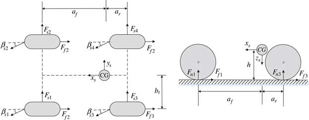
The ground force of the landing gear is shown in Fig. 2. F _n , F _f , F _s denote, respectively, the vertical force, the friction force and the side force. The following assumptions are made in order to simplify the model:

• ∙ The pitch and roll angles are very small.

• ∙ The side-slip angles of tires are very small.

• ∙ The weight and moment of inertia of the tires can be neglected.

• ∙ The tires are modelled as damped springs.

Figure 2

The ground force in top view and left view.

The vertical force of each tire is

(…1) $$F_{{ni}} {\equals}k_{{\delta t}} {\rm \delta }_{{ti}} {\plus}c_{{\delta t}} {\dot{\delta }}_{{ti}} ,\quad i{\equals}1,2,3,4$$

where k _δt is the equivalent stiffness of tires and c _δt is the equivalent damping coefficient of tires. δ _ti and $${\dot{\delta }}_{{ti}} $$ are the compression and the compression, respectively, speed of each tire. We can get the compression of each tire by using UAV states and the geometric parameters of landing gear:

(…2) $$\left\{ {\matrix{ {{\rm \delta }_{{ti}} {\equals}{\rm sat}({\rm \bar{\delta }}_{{ti}} ,0,{\rm inf}),\quad i{\equals}1,2,3,4} \cr {{\rm \bar{\delta }}_{{t1}} {\equals}{\minus}H{\plus}h{\minus}a_{f} \sin {\rm \theta }{\minus}b_{t} \sin \phi } \cr {{\rm \bar{\delta }}_{{t2}} {\equals}{\minus}H{\plus}h{\minus}a_{f} \sin {\rm \theta }{\plus}b_{t} \sin \phi } \cr {{\rm \bar{\delta }}_{{t3}} {\equals}{\minus}H{\plus}h{\plus}a_{r} \sin {\rm \theta }{\minus}b_{t} \sin \phi } \cr {{\rm \bar{\delta }}_{{t4}} {\equals}{\minus}H{\plus}h{\plus}a_{r} \sin {\rm \theta }{\plus}b_{t} \sin \phi } \cr {} \cr } } \right.$$

where H is the distance from the UAV centre of gravity to ground, while h equals to H when δ _ti =0. b _t is the distance between tires and the symmetric plane of the UAV. a _f and a _r are horizontal distance from front tires and rear tires to the center of gravity. Because the compression of tire cannot be less than 0, the amplitude of the compression must be limited by saturation function and defined as

(…3) $${\rm sat}(x,a,b){\equals}\left\{ {\matrix{ {b\quad x\,\gt\,b} \cr {x\quad a\,\lt\,x\,\lt\,b} \cr {a\quad x\,\lt\,a} \cr } } \right.$$

Due to the lack of brake system, the frictional force only contains rolling frictional force which can be expressed as

(…4) $$F_{{fi}} {\equals}{\mu }_{f} F_{{ni}} ,\quad i{\equals}1,2,3,4$$

where μ _f is the frictional coefficient of tires. The study of Zhang⁽ Reference Zhang and Duan ^{5 )} shows that when the side-slip angles of tires are very small, the side force can be approximated as

(…5) $$F_{{si}} {\equals}k_{s} {\rm \beta }_{{si}} F_{{ni}} ,\quad i{\equals}1,2,3,4$$

where k _s and β _s are the cornering stiffness and the slip angle of tires, respectively. As shown in Fig. 2, we can get the side-slip angles:

(…6) $$\left\{ {\matrix{ {{\rm \beta }_{{s1}} {\equals}\arctan \left( {{\minus}(v{\plus}a_{f} r)\,/\,(u{\plus}b_{t} r)} \right)} \cr {{\rm \beta }_{{s2}} {\equals}\arctan \left( {{\minus}(v{\plus}a_{f} r)\,/\,(u{\minus}b_{t} r)} \right)} \cr {{\rm \beta }_{{s3}} {\equals}\arctan \left( {{\minus}(v{\minus}a_{r} r)\,/\,(u{\plus}b_{t} r)} \right)} \cr {{\rm \beta }_{{s4}} {\equals}\arctan \left( {{\minus}(v{\minus}a_{r} r)\,/\,(u{\minus}b_{t} r)} \right)} \cr } } \right.$$

Owing to the fact that the pitch and roll angles are very small, the force and the moment generated by ground are

(…7) $${\mib{F}} _{{b_{t} }} {\equals}\left[ {\matrix{ {{\minus}\mathop{\sum}\limits_{i{\equals}l}^4 {F_{{fi}} } } & {\mathop{\sum}\limits_{i{\equals}1}^4 {F_{{si}} } } & {{\minus}\mathop{\sum}\limits_{i{\equals}1}^4 {F_{{ni}} } } \cr } } \right]^{T} $$

(…8) $${\mib{M}} _{{b_{t} }} {\equals}\left[ {\matrix{ {\left( {F_{{n1}} {\minus}F_{{n2}} {\plus}F_{{n3}} {\minus}F_{{n4}} } \right)b_{t} {\minus}\mathop{\sum}\limits_{i{\equals}1}^4 {F_{{si}} H} } \cr {\left( {F_{{n1}} {\plus}F_{{n2}} } \right)a_{f} {\minus}\left( {F_{{n3}} {\plus}F_{{n4}} } \right)a_{r} {\minus}\mathop{\sum}\limits_{i{\equals}1}^4 {F_{{fi}} H} } \cr {{\minus}\left( {F_{{f1}} {\minus}F_{{f2}} {\plus}F_{{f3}} {\minus}F_{{f4}} } \right)b_{t} } \cr } } \right]$$

2.2 Propeller thrust model

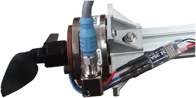
A balance is used to measure the thrusts of the propeller in different throttle at zero inflow speed Fig. 3).

Figure 3

Propeller thrust experiment.

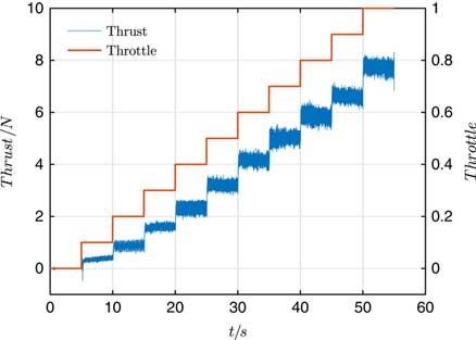
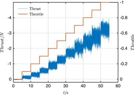
When throttle increases from 0 to 1 in every 5 s with a 0.1 step length, the measured thrust is plotted in Fig. 4. Beard⁽ Reference Beard and Mclain ^{17 )} proposed a simple model for the thrust generated by a propeller

(…9) $$F_{p} {\equals}{1 \over 2}{\rm \rho }S_{p} C_{p} \left( {k_{{p1}} {\rm \delta }_{p} ^{2} {\minus}V_{p}^{2} } \right)$$

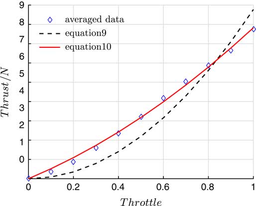
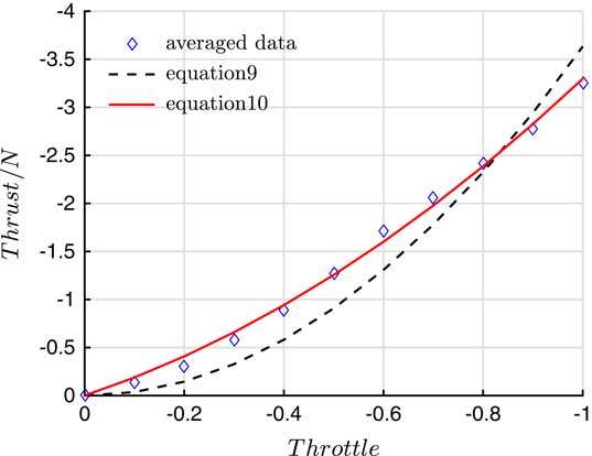
where S _p , C _p and V _p are the disk area, the thrust coefficient and the inflow speed of the propeller, respectively. When the average of thrust is obtained at every throttle, and the data are fitted with the least square method. It is found that the accuracy of fitting is not high enough and an improvement is proposed as

(…10) $$F_{p} {\equals}{1 \over 2}{\rm \rho }S_{p} C_{p} \left( {k_{{p1}} {\rm \delta }_{p} ^{2} {\plus}k_{{p2}} {\rm \delta }_{p} {\minus}V_{p}^{2} } \right)$$

Figure 4

Thrust of the propeller.

The data are fitted again with Equation (10). The R-square of Equation (9) is 0.917, while the R-square of Equation (10) reaches 0.997, showing Equation (10) has a higher fitting precision than Equation (9). The fitting results are shown in Fig. 5.

Figure 5

Data fitting of the thrust.

Without break system, the only way to reduce the aircraft speed is to reverse the propeller. The reverse thrust is shown in Fig. 6. Influenced by the airflow separation of the propeller, the reverse thrust is smaller and contains more noises compared with the forward thrust. The reverse thrust data are fitted with Equations (9) and (10), respectively in Fig. 7. Equation (10) also has a higher fitting precision than Equation (9).

Figure 6

Reverse thrust of the propeller.

Figure 7

Data fitting of the reverse thrust.

Define Δδ _p as the differential throttle, the throttles of left and right propellers are $${\rm \delta }_{{p_{l} }} {\equals}{\rm \delta }_{p} {\plus}\Delta {\rm \delta }_{p} $$ and $${\rm \delta }_{{p_{r} }} {\equals}{\rm \delta }_{p} {\minus}\Delta {\rm \delta }_{p} $$ . Meanwhile, the distance between the propellers and the symmetric plane of the UAV is d _p , thus the V _p of left and right propellers are $$V_{{p_{l} }} {\equals}V_{a} {\plus}d_{p} r$$ and $$V_{{p_{r} }} {\equals}V_{a} {\minus}d_{p} r$$ . The differential thrust of propeller is

$$\Delta F_{p} {\equals}F_{{p_{l} }} {\minus}F_{{p_{r} }} {\equals}{\rm \rho }S_{p} C_{p} (2k_{{p1}} {\rm \delta }_{p} \Delta {\rm \delta }_{p} {\plus}k_{{p2}} \Delta {\rm \delta }_{p} {\minus}2V_{a} d_{p} r)$$

The force and moment generated by propellers are

(…11) $${\mib{F}} _{{b_{p} }} {\equals}\left[ {\matrix{ {F_{{p_{l} }} {\plus}F_{{p_{r} }} } & 0 & 0 \cr } } \right]^{T} $$

(…12) $${\mib{M}} _{{b_{p} }} {\equals}\left[ {\matrix{ 0 & 0 & {\Delta F_{p} d_{p} } \cr } } \right]^{T} $$

2.3 Aerodynamic and gravity model

The aerodynamic forces and moments can be expressed as

(…13) $$\left\{ {\matrix{ {F_{L} {\equals}{1 \over 2}{\rm \rho }V_{a} ^{2} S\left( {C_{L} ({\rm \alpha }){\plus}C_{{L_{q} }} {c \over {2Va}}q} \right)} \vskip--8pt \cr {F_{Y} {\equals}{1 \over 2}{\rm \rho }V_{a} ^{2} S\left( {C_{Y} ({\rm \beta }){\plus}C_{{Y_{p} }} {b \over {2Va}}p{\plus}C_{{Y_{r} }} {b \over {2Va}}r} \right)} \vskip--8pt \cr {F_{D} {\equals}{1 \over 2}{\rm \rho }V_{a} ^{2} S\left( {C_{D} ({\rm \alpha }){\plus}C_{{D_{q} }} {c \over {2Va}}q} \right)} \cr } } \right.$$

(…14) $$\left\{ {\matrix{ {M_{l} {\equals}{1 \over 2}{\rm \rho }V_{a} ^{2} S\left( {C_{l} ({\rm \beta }){\plus}C_{{l_{p} }} {b \over {2Va}}p{\plus}C_{{l_{r} }} {b \over {2Va}}r} \right)} \vskip--8pt \cr {M_{m} {\equals}{1 \over 2}{\rm \rho }V_{a} ^{2} S\left( {C_{m} ({\rm \alpha }){\plus}C_{{m_{q} }} {c \over {2Va}}q} \right)} \vskip--8pt \cr {M_{n} {\equals}{1 \over 2}{\rm \rho }V_{a} ^{2} S\left( {C_{n} ({\rm \beta }){\plus}C_{{n_{p} }} {b \over {2Va}}p{\plus}C_{{n_{r} }} {b \over {2Va}}r} \right)} \cr } } \right.$$

where C _L , C _Y and C _D are aerodynamic lift, lateral and drag forces coefficients, respectively, of the UAV. C _l , C _m and C _n are aerodynamic roll, pitch and yaw moments coefficients, respectively. V _a , S, b and c are the air-speed, the reference area, the wing span and the mean aerodynamic chord of the aircraft, respectively.

Transform the aerodynamic force and moment from the wind frame to the body frame:

(…15) $${\mib{F}} _{{b_{a} }} {\equals}{\rm DCM}_{{bw}} \left[ {\matrix{ {{\minus}F_{D} } & {F_{Y} } & {{\minus}F_{L} } \cr } } \right]^{T} $$

(…16) $${\mib{M}} _{{b_{a} }} {\equals}\left[ {\matrix{ {M_{l} } & {M_{m} } & {M_{n} } \cr } } \right]^{T} $$

Transform the gravity acting on the center of mass to the body frame:

(…17) $${\mib{F}} _{{b_{g} }} {\equals}{\rm DCM}_{{be}} \left[ {\matrix{ 0 & 0 & {mg} \cr } } \right]^{T} $$

2.4 Kinematics and dynamic model

The forces and moments are generated by the ground, propeller propulsion, aerodynamics and gravity

(…18) $$\left\{ {\matrix{ {{\mib{F}} {\equals}{\mib{F}} _{{b_{t} }} {\plus}{\mib{F}} _{{b_{p} }} {\plus}{\mib{F}} _{{b_{a} }} {\plus}{\mib{F}} _{{b_{g} }} } \cr {{\mib{M}} {\equals}{\mib{M}} _{{b_{t} }} {\plus}{\mib{M}} _{{b_{p} }} {\plus}{\mib{M}} _{{b_{a} }} } \cr } } \right.$$

Select the north-east-down positions $${\mib{P}} {\equals}\left[ {\matrix{ {P_{n} } & {P_{e} } & {P_{d} } \cr } } \right]^{T} $$ , body frame velocities $${\mib{V}} _{b} {\equals}\left[ {\matrix{ u & v & w \cr } } \right]^{T} $$ , Euler angles $$\Theta {\equals}\left[ {\matrix{ \phi & \theta & \psi \cr } } \right]^{T} $$ and angular rates $$\Omega {\equals}\left[ {\matrix{ p & q & r \cr } } \right]^{T} $$ as state variables for the UAV, the kinematics and the dynamics of a rigid body can be expressed as

(…19) $$\left\{ {\matrix{ {{\hskip--2pt {\dot{\mib P}}} {\equals}} {DCM_{{be}} ^{T} {\mib{V}}}\hfill \cr {\hskip -3pt{{\dot{\mib V}}} _{b} {\equals}} {{\minus}\Omega {\times}{\mib{V}} _{b} {\plus}{\mib{F}} \,/\,m}\hskip 90 \vskip--8pt \hfill \cr \hskip--1pt {\dot{\Theta }} {\equals} {\left[ {\matrix{ 1 & {\sin \phi \tan {\rm \theta }} & {\cos \phi \tan {\rm \theta }} \cr 0 & {\cos \phi } & {{\minus}\sin \phi } \vskip--6pt \cr 0 & {\displaystyle{{\sin \phi } \over {\cos {\rm \theta }}}} & {\displaystyle{{\cos \phi } \over {\cos {\rm \theta \vskip--5pt }}}}\cr } } \right]{\rm \Omega \hskip 30}} \hfill \cr \hskip--1pt {\dot{\Omega }} {\equals}{J^{{{\minus}1}} \left( {{\minus}{\rm \Omega }{\times}(J{\rm \Omega }){\plus}{\mib{M}} } \right)\hskip 70} \hfill \cr } } \right.$$

3.1 Yaw controller design based on ADRC

In order to design the controller more conveniently, only the yaw angle and the yaw angle rate are taken into consideration, Equation (19) can be simplified as

(…20) $$\left\{ {\matrix{ {} & {\displaystyle{\dot{\psi }}{\equals}{{\sin \phi } \over {\cos {\rm \theta }}}q{\plus}{{\cos \phi } \over {\cos {\rm \theta }}}r} \vskip--12pt \cr {\dot{r}{\equals}} & {\displaystyle{{\left[ {J_{{xx}} (J_{{xx}} {\minus}J_{{yy}} ){\plus}J_{{xz}}^{2} } \right]pq{\minus}J_{{xz}} (J_{{xx}} {\minus}J_{{yy}} {\plus}J_{{zz}} )qr} \over {J_{{xx}} J_{{zz}} {\minus}J_{{xz}}^{2} }}{\plus}{{\left[ {\matrix{ {J_{{xz}} } & 0 & {J_{{xx}} } \cr } } \right]{\mib{M}} } \over {J_{{xx}} J_{{zz}} {\minus}J_{{xz}}^{2} }}} \cr } } \right.$$

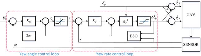
Equation (20) can be considered as two first-order systems in series. According to the time scale separation theory, the yaw angle control loop and yaw angle rate control loop can be designed separately. So the controller is designed on the base of cascade ADRC theory, and the controller structure is shown in Fig. 8

Figure 8

Yaw controller structure.

3.1.1 Yaw angle control loop

Owing to the fact that the pitch and roll angles are quite small, the first item of equation (20) can be further simplified as

(…21) $$\dot{\psi }{\equals}r$$

Since Equation (21) is homogeneous, it’s not necessary to design an ESO for yaw angle control loop. This can not only reduce the amount of computation but also avoid the influence of yaw angle singularity to ESO.

The feedback control law of yaw angular is designed as follows:

(…22) $$\left\{ {\matrix{ {\bar{r}_{c} {\equals}K_{{\rm \psi }} ({\rm \psi }_{c} {\minus}{\rm \psi }{\plus}2\pi n)} \cr {r_{c} {\equals}{\rm sat}(\bar{r}_{c} ,{\minus}r_{{c{\rm max}}} ,r_{{c{\rm max}}} )} \cr } } \right.$$

The maximum yaw angle rate of UAV is finite, therefore, use r _cmax to limit the maximum value of yaw angle command. Because there is a singularity in yaw angle, it is necessary to select the appropriate integer n in order to make the error of yaw angle command and yaw angle within the reasonable range:

(…23) $${\minus}{\rm \pi }\,\lt\,{\rm \psi }_{c} {\minus}{\rm \psi }{\plus}2{\rm \pi }n\,\lt\,{\rm \pi }$$

3.1.2 Yaw angle rate control loop

The second item of Equation (20) can be expressed as

(…24) $$\dot{r}{\equals}f_{r} {\plus}g_{r} \Delta {\rm \delta }_{p} $$

f _r is denoted as the total disturbance. Because of the disturbance on the ground run, f _r is a multi-variable function of both the states and external disturbances. In practice, f _r is complicated and unmeasurable.

g _r is the control efficiency of Δδ _p where

$$g_{r} {\equals}{{J_{{xx}} } \over {J_{{xx}} J_{{zz}} {\minus}J_{{xz}}^{2} }}\left( {{\rm \rho }S_{p} C_{p} (2k_{{p1}} {\rm \delta }_{p} {\plus}k_{{p2}} )} \right)d_{p} $$

as shown in Figs 5 and 7, k _p1 and k _p2 have different values when the throttle is greater or less than zero, and, thus, g _r will change rapidly when the UAV starts using reverse thrust of propeller to slow down. The sharp change of g _r demands a faster response and better robustness of the controller.

The ESO is the key to ADRC, which is able to observe the total disturbance in real time and will be feedback to the control law:

(…25) $$\left\{ {\matrix{ {e_{r} {\equals}\hat{r}{\minus}r} \cr {\dot{\hat{r}}{\equals}\hat{\Delta }_{r} {\minus}{\rm \beta }_{{01}} e_{r} {\plus}g_{r} \Delta {\rm \delta }_{p} } \cr {\dot{\hat{\Delta }}_{r} {\equals}{\minus}{\rm \beta }_{{02}} {\rm fal}(e,{\rm \sigma ,\delta })} \cr } } \right.$$

where $$\hat{\Delta }_{r} $$ is the estimated value of f _r . e _r is the observer error. β₀₁ and β₀₂ are observer gains. Function fal(e, σ, δ) is defined as⁽ Reference Han ^{10 )}

(…26) $${\rm fal}(e,{\rm \sigma ,\delta }){\equals}\left\{ {\matrix{ {\displaystyle{e \over {{\rm \delta }^{{1{\minus}{\rm \sigma }}} }},\quad \mid \! e\!\mid \!\! \hskip--1pt\leq \hskip--1pt {\rm \delta }} \vskip--10pt \cr {\mid\!e\!\mid\,^{{\rm \sigma }} {\rm sign}(e),\quad \,\mid\!e\!\mid\gt\,{\rm \delta }} \cr } } \right.$$

where sign(⋅) is the signum function.

The feedback control law of yaw angular rate is designed as

(…27) $$\left\{ {\matrix{ {\bar{\Delta }{\rm \delta }_{p} {\equals}\left( {K_{r} (r_{c} {\minus}r){\minus}\hat{\Delta }_{r} } \right)g_{r}^{{{\minus}1}} } \cr {\Delta {\rm \delta }_{p} {\equals}{\rm sat}(\bar{\Delta }{\rm \delta }_{p} ,{\minus}\Delta {\rm \delta }_{{p{\rm max}}} ,\Delta {\rm \delta }_{{p{\rm max}}} )} \cr } } \right.$$

To reduce the effect of differential propeller thrust on total thrust, it is necessary to limit the amplitude of differential propeller thrust. Δδ _pmax is the maximum allowable value of Δδ _p while −Δδ _pmax is the minimum value. It is worth noting that Equation (25) must use Δδ _p as an input rather than $$\bar{\Delta }{\rm \delta }_{p} $$ in order to avoid ESO saturation. This is more intuitive and effective than the integral saturation limitation of the PID controller.

3.2 Straight line trajectory tracking controller design based on vector field

Assuming that the error between the yaw angle and the speed yaw angle can be ignored, the distance between UAV and the straight line path is

$$\dot{d}{\equals}V\sin ({\rm \psi }{\minus}{\rm \psi }_{t} )$$

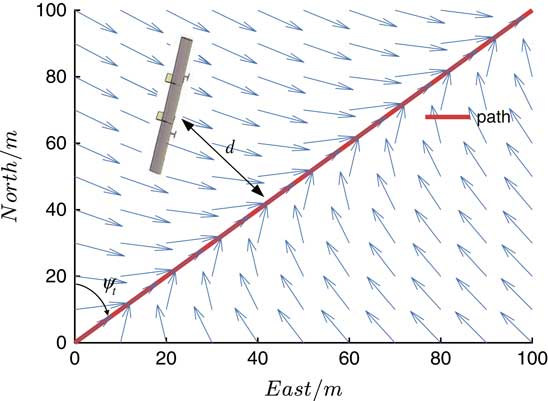
Nelson⁽ Reference Nelson, Barber and Mclain ^{18 )} proposed a path following method based on vector field and gave the proof of stability, and the designed yaw angle command of UAV is given in Equation (28). Sujit⁽ Reference Sujit, Saripalli and Sousa ^{19 )} compared the vector field (VF) path-following control law with non-linear guidance law, vector-field has lower cross-track error. The illustration of the vector-field path-following control is shown in Fig. 9:

(…28) $${\rm \psi }_{c} {\equals}{\rm \psi }_{t} {\minus}{\rm \psi }^{\infty} {2 \over {\rm \pi }}{\tan }^{{\minus}1} (K_{d} d){\plus}2{\rm \pi }l$$

where d is the lateral distance of the UAV from the straight line path, ψ _t is the direction angle of the straight line path, $${\rm \psi }^{\infty} \in\left( {0,{{\rm \pi } \over 2}} \right]$$ is the maximum value of the angle between ψ _c and ψ _t and l is an integer which makes yaw angle command within the reasonable range.

Figure 9

Vector field path following.

It is obvious that Equation (28) is designed for the condition of constant velocity; however, during ground control, the velocity has a wide range of variation. The parameter K _d is redefined to increase the applicability of Equation (28) in practice

(…29) $$K_{d} {\equals}\bar{K}_{d} \,/\,{\rm sat}(V,V_{{{\rm min}}} ,{\rm inf})$$

where V _min is the lowest speed range to avoid singularity.

4.1 Hardware testbed

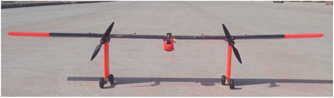
Figure10 shows the UAV used for the ground run tests reported in this paper. The aircraft is made by 3D-printer. The main specifications of this UAV are given in Table 1.

Figure 10

Experimental aircraft.

Table 1

The main specifications of the UAV in this paper

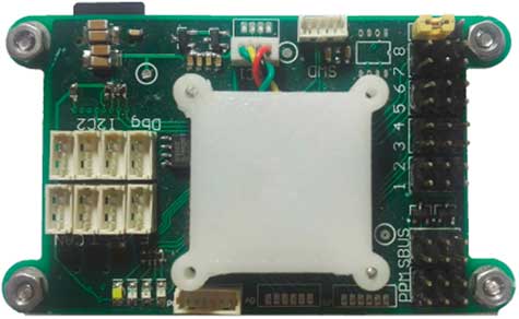
Figure 11 shows the autopilot used in the tests, which is equipped with an arm-cortex-m4 processor, rate gyro, accelerator, magnetic compass and air pressure sensor. Meanwhile, the autopilot is also connected with global positioning system (GPS), air speed sensor, 900MHz radio modem, SBUS/IBUS remote control receiver, electrical motor speed controllers (ESC) and digital servos on the aircraft. The hardware parameters are shown in Table 2.

Figure 11

Autopilot.

Table 2

Autopilot hardware

4.2 Experimental results

To verify the effectiveness, robustness and performance of the proposed ADRC yaw angle controller and the VF straight line trajectory tracking controller for on-ground lateral direction control, experiments have been carried out on the unswept flying-wing UAV, which is introduced in the previous section. At the same time, the PID yaw angle controller with the same gain parameters as the designed yaw angle controller is used for the contrast experiment. The parameter values of the control law used in the experiment are given in Table 3.

Table 3

Parametres of controllers

4.2.1 Experimental results of yaw controller

The performance and robustness of the controller is analysed in three experiments:

(A) Tracking step signal input command

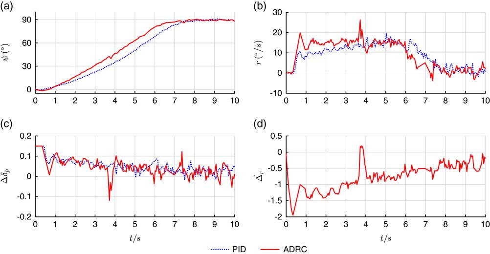
In this experiment, the input command ψ _c is set as step signal with 90° amplitude. The throttle is fixed on 0.3. Figure 12 shows the response comparison between ADRC yaw controller and PID yaw controller.

Figure 12

The response curves of the ADRC and PID yaw controllers when tracking step command.

Figure 12(a) shows that the ADRC yaw angle controller is able to track the input command smoothly and without overshoot. The rise time of ADRC controller is 4.6 s when tracking 90° command, which is smaller than PID controller’s 5.1 s. Meanwhile, the average tracking error from 8 to 10 s of ADRC is 2.34° while that of PID controller is 3.13°; therefore, ADRC yaw angle controller has a better control precision. As shown in Fig. 12(b), yaw rate can reach r _cmax=15°/s within 1 s by using ADRC controller, in stand of 4 s by using PID controller. Figure 12(c) shows that the control output jitter of ADRC controller is bigger than that of PID controller because of ESO observing the ground undulation.

(B) Response to disturbance

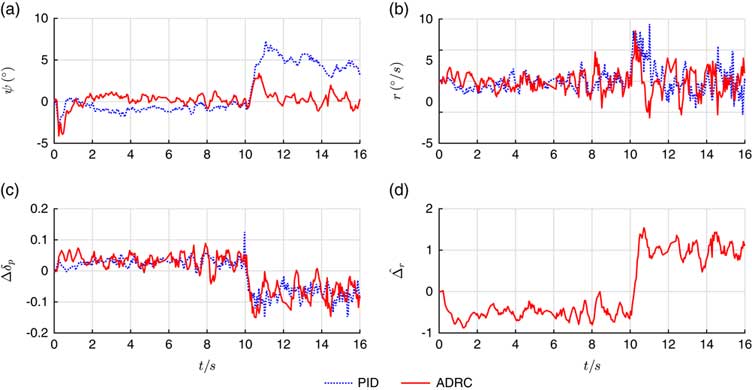
In the process of ground control, there will be many external disturbances. In order to make the experiment more representative, a 0.1 differential propeller thrust is artificially added in the experiment at 10 s. The input command and throttle are fixed on 0 and 0.3 respectively. Figure 13 shows the response results of ADRC and PID yaw controllers.

Figure 13

The response curves of the ADRC and PID yaw controllers after being disturbed.

Figure 13(a) shows that after being disturbed, the ADRC controller can converge quickly and the influence of disturbance is much smaller than that of PID controller, because Fig. 13(d) shows that the ESO observes the disturbance immediately. It can be seen that the ADRC yaw controller has a better robustness than the PID yaw controller.

(C) Response to controller switching

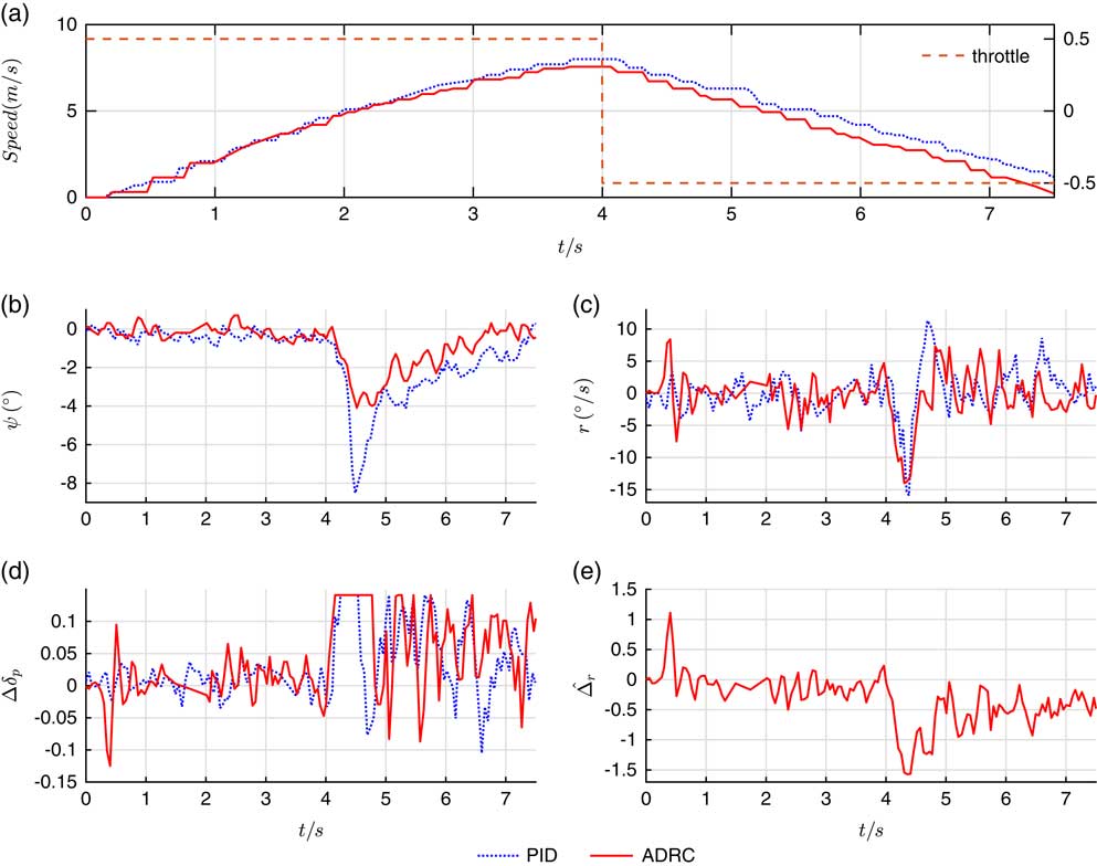
An experiment is designed to test the yaw controller efficiency when the UAV is reducing speed. During the first 4 s of the experiment, 0.5 throttle is used to accelerate the speed, then −0.5 throttle is used to decelerate. Because the rotating speed of the propeller varies greatly, there is a strong non-linearity in thrust and reverse thrust switching. In the process of switching, the controllability of the aircraft is very weak. Figure 14 shows the responses of ADRC and PID yaw controllers.

Figure 14

The response curves of the ADRC and PID yaw controllers during the process of reducing speed.

Figure 14(a) shows the speed of UAV measured by GPS. As shown in Fig. 14(b), because of the incomplete symmetry of UAV, the UAV turns left at the beginning of the switching. Meanwhile, in Fig. 14(c), the ADRC controller outputs the maximum differential propeller thrust immediately while the PID controller is obviously much slower. Figure 14(b) shows that due to better robustness and faster response speed, the maximum tracking error of ADRC yaw controller is half of that of the PID controller.

4.2.2 Vector field straight line trajectory tracking controller

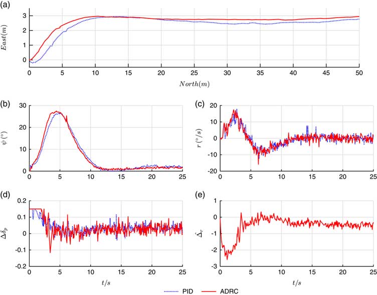
Figure 15 shows the experimental results of trajectory tracking controllers which uses ADRC and PID controllers as inner loop when tracking 3m step command.

Figure 15

The response curves of straight line trajectory tracking controllers.

Figure 15(a) shows that vector field trajectory tracking controller is able to track the straight line, and, at the same time, when ADRC is used as the inner loop controller, it has better rate of convergence and control accuracy than the PID controller. Because of the small error between the yaw angle measured by attitude and heading reference system (AHRS) and the actual yaw angle, a static-state error exists in the experiment. But considering the accuracy of GPS, this static-state error is in an acceptable range.