1. Introduction
Bubble flow generated by gas injection into liquids reflects typical gas–liquid two-phase flow characterised by a continuous liquid phase and dispersed gas phase. Owing to its high efficiency in mixing and heat transfer as well as its ease of generation, it has been widely applied in environmental engineering, chemical processing and marine engineering (Risso Reference Risso2018; Alméras et al. Reference Alméras, Mathai, Sun and Lohse2019). The formation and release of bubbles from submerged orifices in quiescent fluids constitutes a fundamental area of gas–liquid two-phase flow research that impacts industrial equipment such as bubble columns, slurry bed reactors and gas–liquid stirred tanks (Qu, Yu & Zhang Reference Qu, Yu and Zhang2017). For instance, Navisa et al. (Reference Navisa, Sravya, Swetha and Venkatesan2014) demonstrated that injecting air into liquids can significantly increase the dissolved oxygen content, thereby improving the aquatic environment. In aerospace thermal control systems, the gas–liquid phase transition and bubble-driven flow are utilised to significantly enhance heat exchange efficiency (Lee, Mudawar & Hasan Reference Lee, Mudawar and Hasan2016). Consequently, investigating bubble behaviour and its induced flow characteristics – especially bubble entrainment properties – holds both key theoretical and practical significance.
In quiescent fluids, the path instability of freely rising millimetre-sized bubbles has attracted considerable attention owing to the complex link between gas–liquid interface dynamics and surrounding flow structures. Subsequent to initial rectilinear rise, bubbles often exhibit nonlinear trajectories such as zigzag, spiral (Duineveld Reference Duineveld1995; De Vries Reference De Vries2001; Tripathi, Sahu & Govindarajan Reference Tripathi, Sahu and Govindarajan2015) or chaotic motions (Cano-Lozano et al. Reference Cano-Lozano, Martínez-Bazán, Magnaudet and Tchoufag2016; Bonnefis, Fabre & Magnaudet Reference Bonnefis, Fabre and Magnaudet2023). These types of motion are governed by the interaction between bubble deformation and its wake. Veldhuis, Biesheuvel & Wijngaarden (Reference Veldhuis, Biesheuvel and Wijngaarden2008) demonstrated that the three-dimensional (3-D) paths of rising bubbles result from superimposed oscillation modes with phase differences. Surface vorticity and pressure imbalances further contribute to instability by enhancing wake strength and bubble-flow coupling (Joshi et al. Reference Joshi, Nandakumar, Evans, Pareek, Gumulya, Sathe and Khanwale2017; Bonnefis et al. Reference Bonnefis, Fabre and Magnaudet2023).
Bubble morphology is a critical factor that influences rising behaviour. Spherical and spherical-cap bubbles typically follow along rectilinear paths, whereas ellipsoidal bubbles are prone to unstable trajectories such as zigzag or spiral motions (Clift, Grace & Weber Reference Clift, Grace and Weber1978; Takagi, Prosperetti & Matsumoto Reference Takagi, Prosperetti and Matsumoto1994; Magnaudet & Eames Reference Magnaudet and Eames2000). Lalanne et al. (Reference Lalanne, Abi Chebel, Vejražka, Tanguy, Masbernat and Risso2015) established a link between path oscillations and spherical harmonic surface vibrations. Numerical simulations have demonstrated that the Eötvös number (Eo), which characterises the balance between buoyancy and surface tension, governs bubble surface curvature and therefore affects trajectory stability (Zhang et al. Reference Zhang, Ni and Magnaudet2021, Reference Zhang, Ni and Magnaudet2022). Recent 3-D imaging conducted by Feng, Wang & Zhao (Reference Feng, Wang and Zhao2023) also showed that increasing the size of the bubble lowers its oscillation frequency through inertia and interfacial force changes across scales. Bubble morphology and initial development are strongly affected by orifice parameters. Among them, orifice diameter has been the main focus in previous studies. For example, di Bari & Robinson (Reference di Bari and Robinson2013) reported that smaller orifices generate bubbles with smaller volumes, shorter detachment times and more spherical shapes. However, few studies have focused on the geometric shape of the orifice. In practical systems, the geometry of the orifice governs the initial gas–liquid interface configuration and contact angle distribution, which, in turn, determines the surface tension field during bubble growth. This anisotropic interfacial tension can cause non-uniform deformation upon detachment and alter the subsequent bubble dynamics (Hanafizadeh et al. Reference Hanafizadeh, Sattari, Hosseini-Doost, Nouri and Ashjaee2018). Therefore, investigating the effect of orifice geometry on bubble morphology, path stability and induced flow remains an important yet underexplored topic.
To further understand the role of orifice geometry in trajectory instability, researchers have visualised bubble-induced wake structures. Brücker (Reference Brücker1999) identified periodic hairpin vortex shedding as the cause of lateral deviation. Furthermore, direct numerical simulations have confirmed that vortex asymmetry leads to periodic shape oscillations (Gaudlitz & Adams Reference Gaudlitz and Adams2009), whereas particle image velocimetry (PIV) revealed complex 3-D vortex tube structures in the wake of oscillating bubbles (Zenit & Magnaudet Reference Zenit and Magnaudet2009). She et al. (Reference She, Gao, Zuo, Liao, Zhao, Zhang, Nie and Shao2021) demonstrated the stage-dependent vortex evolution via tomographic PIV, and Cao & Macián-Juan (Reference Cao and Macián-Juan2021) established a relationship between vortex asymmetry and trajectory curvature. Numerical studies by Shi et al. (Reference Shi, Zhang and Magnaudet2024, Reference Shi, Zhang and Magnaudet2025) further demonstrated that the shedding and regeneration of wake vortices could lead to abrupt bubble jumping near the boundaries. These insights highlight the critical influence of initial bubble conditions – particularly those determined by orifice geometry – on the evolution of the bubble-wake interactions.
When bubble motion intensifies, the induced liquid flow exhibits marked turbulence characteristics, known as bubble-induced turbulence (BIT). Early measurements by Michiyoshi & Serizawa (Reference Michiyoshi and Serizawa1986) demonstrated that bubbles can significantly enhance velocity fluctuations, thereby promoting turbulence development. Although subsequent study by So et al. (Reference So, Morikita, Takagi and Matsumoto2002) showed that bubbles near solid walls partially suppress turbulence fluctuations, this suppression diminishes at higher void fractions, with the Reynolds stress distribution of BIT becoming similar to that of single-phase turbulent flow (Kim, Lee & Park Reference Kim, Lee and Park2016). Aliyu et al. (Reference Aliyu, Seo, Kim and Kim2018) reported significant increases in the turbulent kinetic energy of BIT with increasing bubble flow rates and axial positions, and Alméras et al. (Reference Alméras, Mathai, Sun and Lohse2019) demonstrated a nonlinear relationship between the turbulent diffusion coefficients and void fractions. Wu et al. (Reference Wu, Wang, DiMarco and Tan2021) experimentally investigated bubble plume turbulence in stationary fluids, noting significant differences in plume growth depending on the bubble size and quantity. As regards the energy spectrum of turbulence, Lance & Bataille (Reference Lance and Bataille1991) reported deviations from the traditional Kolmogorov −5/3 scaling law owing to the presence of bubbles. Similarly, Rensen, Luther & Lohse (Reference Rensen, Luther and Lohse2005) observed spectra with slopes smaller than −5/3, attributing these to additional energy input from bubble motions. Prakash et al. (Reference Prakash, Mercado, Wijngaarden, Mancilla, Tagawa, Lohse and Sun2016) found that the fluctuating energy spectra exhibited a slope of −3 at scales smaller than the bubble size. Using direct numerical simulation, Pandey, Ramadugu & Perlekar (Reference Pandey, Ramadugu and Perlekar2020) further confirmed that the turbulent bubbly flow energy spectra can deviate below the −5/3 slope. Wang & Socolofsky (Reference Wang and Socolofsky2019) performed experiments in low-void-fraction bubble chains. The scale of the bubble wakes had an upper limit (e.g. slopes of −3 or −8/3) to deviations below −5/3, whereas larger-scale spectra reverted to the traditional −5/3 law. Current studies on BIT have predominantly focused on the statistical characteristics of macroscopic turbulence quantities, whereas detailed insights into the internal flow structures remain limited. Therefore, this study applied the turbulent/non-turbulent interface (TNTI) framework to analyse the local structural features of BIT. A TNTI is a thin instantaneous fluid layer that separates turbulent and non-turbulent regions and is widely encountered in various natural and engineering flows (Da Silva et al. Reference Da Silva, Hunt, Eames and Westerweel2014; Mellado Reference Mellado2017). Hydrodynamics near the TNTI strongly influence the transport processes of mass, momentum, energy and scalars across the interface, controlling turbulence growth, diffusion, mixing and reaction rates.
In summary, although significant progress has been made in understanding bubble morphology, trajectories and induced flow characteristics in quiescent fluids, detailed experimental studies on effects of orifice shape on bubble motion and induced flow structures remain insufficient because of the sensitivity of gas–liquid two-phase flow parameters and complex flow structures. Thus, this study employs shadowgraphy and laser-induced fluorescence PIV (LIF-PIV) to experimentally investigate bubble continuous free-rise processes and induced flow fields in quiescent fluids, quantitatively analysing the bubble morphology in three dimensions and flow field characteristics in two dimensions. With an emphasis on the effects of orifice geometry, this study aims to elucidate the underlying fluid-mechanical mechanisms. This paper is organised as follows. Section 2 presents the experimental set-up. Section 3.1 investigates bubble morphology, including contact angles during the formation stage and shape oscillations during the ascent. The characteristics of bubble motion and force budget are explored in § 3.2, while § 3.3 presents the bubble-induced flow field structure. Section 3.4 discusses BIT characteristics in relation to the TNTI. Finally, the paper concludes in § 4 . Appendices A and B provide details on the 3-D reconstruction of bubbles and the TNTI interface identification technique, respectively.
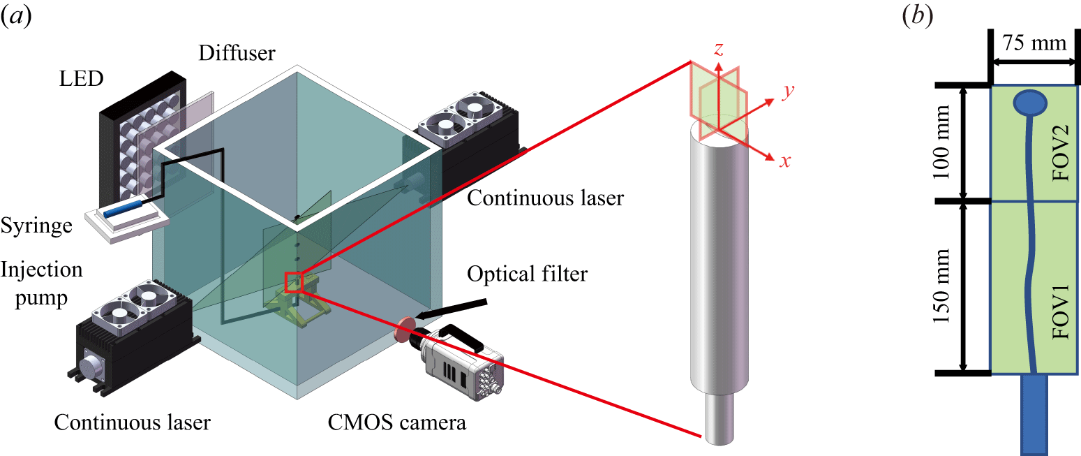
(a) Shadowgraphy set-up; (b) circular orifice (AR = 1); (c) elliptical orifice (AR = 2); (d) elliptical orifice (AR = 3); (e) elliptical orifice (AR = 4).

2. Experiment set-up
The experiment was conducted in a transparent Plexiglas tank with dimensions of 600 mm
 $\times$
600 mm
 $\times$
600 mm and a wall thickness of 20 mm, as shown in figure 1(a). The tank was sufficiently large (approximately 200 times the inner diameter of the orifice) to minimise the influence of the tank walls on both the bubble motion and bubble-induced flow field. The bubble-generation system included a syringe pump, syringe, ventilation tube and an orifice fixation device. To assess the effects of geometry while controlling size, the same equivalent diameter (
 $D_n$
= 4 mm) was applied to all orifices, including circular (AR = 1) and elliptical (AR = 2–4) configurations, as shown in figure 1(b–e). The orifice was positioned central to the four walls, 70 mm above the bottom surface and approximately 520 mm below the free liquid surface, allowing the bubbles to reach a steady state during the final stage of their ascent (Li, Xu & Wang Reference Li, Xu and Wang2021; Wang et al. Reference Wang, Xu, Li and Wang2024). The gas flow rate
 $Q_g$
was controlled by a high-precision medical syringe pump (LSP02-1B, Baoding Longer Precision Pump Co. Ltd.), which drove a syringe with an inner diameter of 30 mm. The linear speed of the syringe pump was adjustable with a resolution of 5
 $\unicode {x03BC}$
m min−1, corresponding to a flow accuracy of 3.5
 $\unicode {x03BC}$
l min−1. In this study,
 $Q_g$
= 50 ml min−1 was selected, which has been identified as a suitable operating condition for such experiments (Wang et al. Reference Wang, Xu, Li and Wang2024).
To obtain the morphological characteristics of the bubbles, shadowgraphy was employed in this experiment to capture bubble shadow images from an orthogonal view, similarly to the methods used by She et al. (Reference She, Gao, Zuo, Liao, Zhao, Zhang, Nie and Shao2021) and Lee & Park (Reference Lee and Park2022). This approach was chosen because of the strong 3-D nature of bubble motion during ascent (Tripathi et al. Reference Tripathi, Sahu and Govindarajan2015; Cano-Lozano et al. Reference Cano-Lozano, Martínez-Bazán, Magnaudet and Tchoufag2016). The chosen method can capture both the 3-D shape and trajectory of the bubbles. The specific 3-D reconstruction algorithm is provided in Appendix A. The shadow imaging system mainly consisted of two high-speed complementary metal oxide semiconductor (CMOS) cameras, two diffuser plates and two light-emitting diode (LED) lamps. The LED lamps provided continuous illumination. The two high-speed CMOS cameras (Photron Nova R2 high-speed cameras with Nikon 50 mm f/1.8D lenses, frame rate = 1000 f.p.s.) were arranged perpendicular to the tank. The CMOS cameras had a resolution of 1024
 $\times$
2048 pixels and magnification of 0.074 mm per pixel (denoted as
 $M_b$
). The measurement field of view (FOV) covered a radius of 75 mm in the radial direction (
 $x$
or
 $y$
, where
 $x$
and
 $y$
are the major and minor axis directions of the orifice, respectively) and 150 mm in the axial direction (
 $z$
), as shown in figure 2(b). Based on the literature (Elsinga et al. Reference Elsinga, Scarano, Wieneke and Van Oudheusden2006; Raffel et al. Reference Raffel, Willert, Scarano, Kähler, Wereley and Kompenhans2018), the maximum absolute uncertainty of displacement was accepted as 0.1 pixel. Based on the standard relation
 $\varepsilon _x=\varepsilon _{x,{pix}}\,M_b$
with
 $\varepsilon _{x,{pix}}=0.1$
pixel, and noting that the two cameras were operated with identical image resolution and physical FOV, the magnification
 $M_b$
is identical for both views; consequently, the absolute displacement uncertainties of the two cameras are identical, and reporting a single value is sufficient. Considering image magnification, the absolute displacement uncertainty
 $\varepsilon _{x1}$
was 7.4
 $\times 10^{-3}$
mm. The relative uncertainty was obtained by non-dimensionalising this value using the bubble diameter measured via shadowgraphy, yielding a range between 0.11 %–0.13 %. The cameras were synchronised and activated by a MicroPulse 725 synchroniser (MicroVec, Inc.), with a maximum control error of no more than 0.25 ns and control precision six orders of magnitude higher than the synchronisation sampling frequency.
The (a) LIF-PIV set-up; (b) FOV.

For the flow field measurements, LIF-PIV was employed to obtain quantitative information regarding the bubbles and their induced flow fields. To eliminate the shadows caused by bubble occlusion, two continuous lasers with a power of 8 W and wavelength of 532 nm were used to illuminate the flow field from both sides of the water tank. The laser sheet was positioned in the
 ${\textit{zx}}$
or
 ${\textit{zy}}$
coordinate plane, alternately capturing the plane of the major and minor axes of the orifice, with the origin defined as the centre of the orifice. To capture the morphology of the bubbles more clearly during flow field measurements, an LED array was positioned opposite the camera. Fluorescent particles (PMMA Rhodamine B) with a nominal diameter of 7
 $\unicode {x03BC}$
m were used as PIV tracking particles, emitting fluorescence at 590 nm when excited by a 532 nm laser. The influence of tracer particles – which may introduce surfactant-like effects – on the bubble dynamics was assessed by comparing the measured bubble terminal velocity (§ 3.2.1) with the theoretical prediction by Tomiyama et al. (Reference Tomiyama, Celata, Hosokawa and Yoshida2002). The deviation remained within 10 %, indicating that the tracer-induced effect on bubble motion was negligible. The high-speed CMOS camera (Photron Nova R2) was used to record images of the tracer particles. A high-pass filter with a cutoff wavelength of 560 nm was placed in front of the lens to eliminate strong reflections from the laser at the gas–liquid interface and interference from ambient light sources.
Flow field information was captured in two FOVs: FOV1 was near the orifice and overlapped with the bubble region captured using the shadowgraphy method. The magnification and lens parameters for these measurements were identical to those used in the bubble shadow experiment. Then FOV2 was located farther from the orifice, where the bubbles fully entered the oscillatory ascent stage. This region required a higher quality image; therefore, a Nikon 105 mm f/3.5–4.5D lens was used, with a resolution of 1536
 $\times$
2048 pixels and magnification of 0.049 mm per pixel. The measurement FOV covered a radius of 75 mm in the radial direction (
 $x$
or
 $y$
) and 100 mm in the axial direction (
 $z$
). The absolute displacement uncertainty in FOV2 was
 $\varepsilon _{x2}$
= 4.9
 $\times 10^{-3}$
mm. This value was non-dimensionalised using the bubble diameter obtained via shadowgraphy, resulting in a relative uncertainty of 0.07 %–0.09 %. The acquisition frequency for both FOV1 and FOV2 was 1000 Hz, with an acquisition time exceeding 21 s for FOV1 and 16 s for FOV2, allowing the capture of 16 000 frames in a single operation and ensuring the convergence of the time-averaged flow field (Wang et al. Reference Wang, Xu, Li and Wang2024).
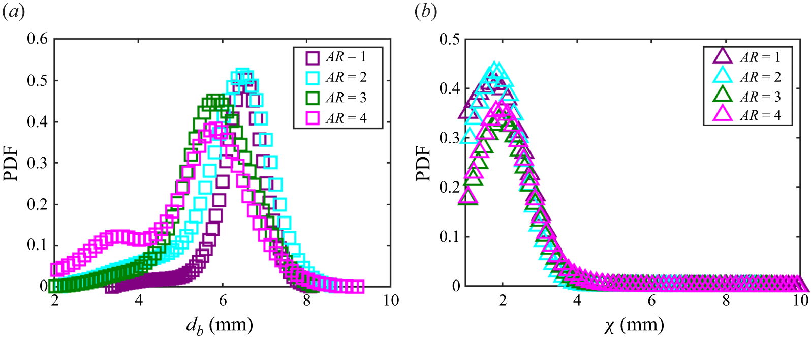
The PDF of the (a) equivalent bubble diameter (
 $d_b$
), and (b) bubble AR (
 $\chi$
).

3. Results and discussion
3.1. Bubble morphology
The bubble morphology was quantified from the measured bubble volume (
 $Vol_b$
) obtained using the image-processing procedure described in Appendix A. The equivalent bubble diameter (
 $d_b$
) and the bubble aspect ratio (AR) (
 $\chi$
) were calculated using (3.1) and (3.2), where
 $d_l$
and
 $d_s$
represent the major and minor bubble axes, respectively. Probability density functions (PDF) of
 $d_b$
and
 $\chi$
are presented in figure 3, and the corresponding statistics are listed in table 1. As the orifice AR increases, the mean
 $d_b$
decreases, whereas the standard deviation increases. The mean
 $\chi$
and standard deviation increase with AR. These trends indicate that a higher AR reduces the overall bubble size while increasing morphological variability. Moreover, the distributions at AR = 2 are comparable to those for the circular orifice (AR = 1); more pronounced differences appear for AR
 $\geqslant$
3, with the AR = 3 and AR = 4 cases exhibiting similar statistics:
Statistical parameters of bubble morphology.

 \begin{align} d_b &=\sqrt [3]{\left (\left (\frac {\left (Vol_b\right )6}{\pi}\right )\right )}, \end{align}
 \begin{align} \chi &=d_l/d_s. \end{align}
Figure 4 shows the shape of the bubble near the orifice. The bubbles generated from the circular orifice exhibit a relatively uniform shape, whereas those generated from the elliptical orifice vary considerably. These differences arise during both the formation and rising stages, the formation stage being primarily influenced by the contact angle at the orifice and the rising stage being primarily influenced by shape oscillations during ascent. The bubble shapes from the two planes at AR = 2 are relatively similar; however, at AR
 $\geqslant$
3, notable differences can be observed between the major- and minor-axis planes. At both AR = 3 and AR = 4, the bubbles in the
 ${\textit{zx}}$
-plane appear elongated, whereas those in the
 ${\textit{zy}}$
-plane are smaller. Therefore, a detailed analysis of the two mechanisms is presented in §§ 3.1.1 and 3.1.3, with a focus on the circular orifice (AR = 1) and elliptical orifice (AR = 3) cases.
Schematic of the bubble shapes. Bubbles generated from (a) a circular orifice (AR = 1), (b) an elliptical orifice (AR = 2), (c) an elliptical orifice (AR = 3) and (d) an elliptical orifice (AR = 4). Here (i) major-axis plane (
 ${\textit{zx}}$
); (ii) minor-axis plane (
 ${\textit{zy}}$
).

3.1.1. Bubble contact angle
The bubble formation process is typically divided into three stages: weeping, expansion and detachment (Hanafizadeh et al. Reference Hanafizadeh, Sattari, Hosseini-Doost, Nouri and Ashjaee2018). These stages are characterised by different equilibria between buoyancy and surface tension, with significant morphological changes such as neck formation, which occurs primarily during the final stage. Among the various morphological formation features, contact angle plays a particularly important role (Wang, Xu & Wang Reference Wang, Xu and Li2025a
). As shown in figure 4, the main difference in bubble shape between the major- (
 ${\textit{zx}}$
) and minor-axis (
 ${\textit{zy}}$
) planes of the elliptical orifice is the contact angle
 $\phi$
. To quantitatively assess this difference, the contact angles during the formation process were statistically analysed. Because the bubbles exhibited minimal growth during the weeping stage, the contact angle remained nearly constant; thus, the analysis focused on the expansion and detachment stages. The bubble contours were extracted and fitted with curves, and the contact angle was determined from a 50
 $\times$
50 pixel region (3.7
 $\times$
3.7 mm) near the bubble base by calculating the angle between the tangents to the contour and horizontal plane, as shown in figure 5 (di Bari & Robinson Reference di Bari and Robinson2013).
Schematic of the bubble contact angles during the formation process: (a) weeping, (b) expansion and (c) detachment stages.

Figure 6(a) shows the variations in contact angles for the bubbles generated from the circular orifice. The contact angle trends in both the
 ${\textit{zx}}$
plane (major-axis direction) and
 ${\textit{zy}}$
plane (minor-axis direction) are generally consistent. After the weeping stage, the bubbles enter the expansion stage. As the bubble volume increases, buoyancy becomes dominant and the initially flattened bubble becomes more spherical, leading to a rapid increase in the contact angle. Once the contact angle exceeds a certain threshold, the interfacial tension and pressure balance cause the contact area at the bubble base to shrink, resulting in a slight decrease in the contact angle. With continued contraction and an increasing bottom curvature, the contact angle gradually increases. Upon reaching the critical contraction, the bubble enters the detachment stage, during which a neck forms and progressively narrows. Thus, a sharp decrease in the contact angle occurs until the bubbles detached (di Bari & Robinson Reference di Bari and Robinson2013).
Contact angles of the bubbles during the formation process: (a) circular orifice with AR = 1; (b) elliptical orifice with AR = 3; (c) force diagram during the bubble formation phase.

Figure 6(b) shows the evolution of the contact angles of the bubbles from the elliptical orifice. Significant differences between the
 ${\textit{zx}}$
and
 ${\textit{zy}}$
planes can be observed, particularly in the weeping and expansion stages. Bubbles in the
 ${\textit{zy}}$
plane expand earlier, resulting in a gradual increase in the contact angle, whereas those in the
 ${\textit{zx}}$
plane remain almost unchanged. This behaviour stems from the narrower width along the minor axis, which imposes stronger lateral confinement and promotes vertical growth, thus accelerating the onset of expansion (Tsuge, Tezuka & Mitsudani Reference Tsuge, Tezuka and Mitsudani2006). In the early expansion phase, the contact angle in the
 ${\textit{zy}}$
plane is slightly higher owing to the greater local curvature and interfacial tension associated with a smaller aperture. As the bubble continues to grow, the contact line starts to contract more rapidly along the minor axis, leading to a more pronounced decrease in the contact angle (Chen & Groll Reference Chen and Groll2006). Despite starting at a higher value, the contact angle in the
 ${\textit{zy}}$
plane eventually decreases below that in the
 ${\textit{zx}}$
plane. During neck formation in the detachment stage, the contact angles in both planes decline sharply and converge.
The anisotropic evolution of the contact angle in elliptical orifices has two key effects. First, the average contact angle is smaller than that of circular orifices, leading to reduced bubble detachment sizes. As illustrated in figure 6(c), the formation process is governed by the balance among buoyancy
 $F_B$
, gas-injection momentum
 $F_M$
, hydrodynamic drag
 $F_D$
, inertia
 $F_I$
and surface tension
 $F_\sigma$
. Specifically, detachment is controlled by the competition between
 $F_B$
and the effective capillary attachment at the contact line (Kim, Kamotani & Ostrach Reference Kim, Kamotani and Ostrach1994; Lv et al. Reference Lv, The, Eijkel, Van Den Berg, Zhang and Lohse2017; Wang et al. Reference Wang, Xu and Li2025a
). Although the surface tension coefficient
 $\sigma$
is constant, the elliptical orifices exhibit a systematically smaller dynamic contact angle. This reduces the vertical capillary force opposing detachment, allowing buoyancy to overcome the attachment force at a smaller bubble volume. Consistent with this mechanism, figure 7 shows that the bubble-release frequency increases with the orifice AR, indicating a shorter formation period. This trend matches the decrease in detached bubble diameter reported in § 3.1. Second, the non-uniform distribution of capillary forces caused by the asymmetric contact angle promotes rapid bubble deformation immediately upon detachment. Further discussion on postdetachment deformation is presented in § 3.1.3 (Oguz & Prosperetti Reference Oguz and Prosperetti1993).
Bubble formation frequency: (a) AR = 1; (b) AR = 2; (c) AR = 3; (d) AR = 4.

3.1.2. Bubble curvature
To quantify whether the differences established during bubble formation persist during ascent and lead to interfacial anisotropy, we analyse the interfacial curvature and its symmetry. Curvature not only provides a quantitative measure of bubble-shape variation, but also helps interpret the accompanying changes in bubble motion, because capillary forces enter the vorticity budget through curvature-dependent terms. To clarify the physical mechanism, we therefore report the vorticity-generation relation of Magnaudet & Mercier (Reference Magnaudet and Mercier2020) together with the associated curvature statistics; the full variable definitions are as follows:
 \begin{equation} \frac {{\textrm D}\boldsymbol{\omega }}{{\textrm D}t} = \boldsymbol{\omega }\boldsymbol{\cdot }\boldsymbol{\nabla }\boldsymbol{u} -\boldsymbol{\nabla }\times \! \left (\frac {\mu }{\rho _l}\boldsymbol{\nabla }\times \boldsymbol{\omega }\! \right ) +\frac {\boldsymbol{\nabla }\rho _l}{\rho _l^{2}}\times \boldsymbol{\nabla }p +2\boldsymbol{\nabla }\times \left (\frac {\boldsymbol{\nabla }\mu }{\rho _l}\boldsymbol{\cdot }\boldsymbol{\varSigma }\right ) -\boldsymbol{\nabla }\left (\frac {\sigma }{\rho _l}\kappa \right )\times \boldsymbol{n}\,\delta _s, \end{equation}
where
 $\boldsymbol{\omega }$
is the vorticity in the surrounding liquid,
 $\boldsymbol{u}$
is the liquid velocity,
 $p$
is the pressure,
 $\sigma$
is the surface-tension coefficient,
 $\rho _l$
is the liquid density,
 $\kappa$
is the bubble-interface curvature,
 $\boldsymbol{n}$
is the unit normal to the interface and
 $\boldsymbol{\varSigma }=({1}/{2})(\boldsymbol{\nabla }\boldsymbol{u}+(\boldsymbol{\nabla }\boldsymbol{u})^{T})$
is the strain-rate tensor. The function
 $\delta _s$
is non-zero only at the gas–liquid interface and localises the action of surface tension. The last term in (3.3), driven by
 $\kappa$
, represents the surface-tension-dominated source of vorticity generation. In our experiments, temperature variations were negligible, and
 $\sigma$
can therefore be treated as constant. Consequently, the symmetry of the curvature field
 $\kappa$
directly controls the spatial distribution of capillary vorticity production and, in turn, the organisation of the wake. Accordingly, curvature statistics are evaluated using arclength-weighted definitions,
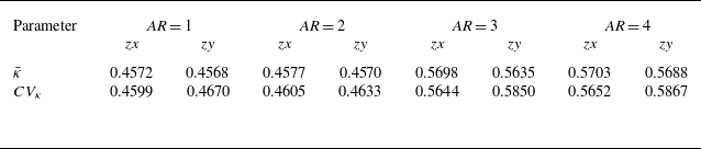
 \begin{align} &\hspace{1.00cm} \bar {\kappa } =\frac {1}{L}\sum _{i=1}^{N}\left |\kappa _i\right |\Delta l_i, \end{align}
 \begin{align} & {\textrm{Std}}_{\kappa } = \sqrt {\frac {1}{L}\sum _{i=1}^{N}\left (\left |\kappa _i\right |-\bar {\kappa }\right )^{2}\Delta l_i}, \end{align}
 \begin{align} &\hspace{1.00cm} \textit{CV}_{\kappa } =\frac {{\textrm{Std}}_{\kappa }}{\bar {\kappa }}, \end{align}
where
 $L=\sum _{i=1}^{N}\Delta l_i$
is the total arclength of the bubble contour in the corresponding projection plane. Since path instability results from symmetry breaking, comparing the
 ${\textit{zx}}$
and
 ${\textit{zy}}$
projections serves as a direct measure of interfacial anisotropy, effectively capturing the asymmetry of the 3-D interface. The statistical results are summarised in table 2. Figure 8 shows the height variation of curvature for AR = 1 and AR = 3. Bubbles generated by circular orifices show nearly isotropic curvature statistics in the two orthogonal planes. This implies a more uniform capillary action along the interface. In contrast, elliptical orifices lead to clear curvature anisotropy, which promotes wake asymmetry and zigzag trajectories (Wang et al. Reference Wang, Xu, Li and Wang2024). This agrees with Liu et al. (Reference Liu, Cong, Song, Wu and Chen2022), who reported higher morphological symmetry and higher motion stability for bubbles from circular orifices, and stronger asymmetry for elliptical-orifice bubbles during generation and ascent.
Statistical results of mean absolute curvature
 $\bar {\kappa }$
and
 $CV_{\kappa }$
.

Variation of mean absolute curvature and curvature coefficient of variation with rise height: (a,b)
 $\bar {\kappa }$
, (c,d)
 $CV_{\kappa }$
. Here (a,c) circular orifice (
 $\textit{AR}=1$
); (b,d) elliptical orifice (
 $\textit{AR}=3$
).

3.1.3. Bubble deformation mode
Bubbles exhibit significant morphological oscillations during their ascent, hindering the comprehensive characterisation of bubble shapes solely through the statistical analysis of bubble size. Modal decomposition can better reflect bubble shape characteristics (Lalanne et al. Reference Lalanne, Abi Chebel, Vejražka, Tanguy, Masbernat and Risso2015); therefore, Fourier decomposition was employed to evaluate the bubble shape variations. Fourier decomposition represents bubble surface oscillations as a combination of sinusoidal and cosinusoidal oscillations with various frequencies. The origin of the polar coordinate system was set at the mean position (
 $x_c$
,
 $y_c$
) of the bubble contour in the Cartesian coordinate system. The mathematical formulae are expressed in (3.7)–(3.9), where
 $\theta \in [0,\ 2\pi )$
denotes the polar angle, and
 $a_n$
and
 $b_n$
represent the Fourier coefficients of cosine and sine, respectively. This method comprises several steps. First, bubble contours are identified based on two-dimensional (2-D) contour recognition. Thereafter, the piecewise cubic Hermite interpolating polynomial method is employed to interpolate the contours, ensure smoothness, and eliminate fluctuations or saddle points (Fritsch & Carlson Reference Fritsch and Carlson1980). Finally, the bubble contour is reconstructed using the Fourier method expressed in (3.9). Figure 9 shows the reconstructed bubble contours obtained from the first ten Fourier modes. The results indicate that Fourier modal reconstruction effectively captures the bubble shape, maintaining a low reconstruction error even for complex bubble geometries,
 \begin{align} x_c &=\frac {1}{N}\sum _{i=1}^{N}x_i, \end{align}
 \begin{align} y_c &=\frac {1}{N}\sum _{i=1}^{N}y_i, \end{align}
 \begin{align} r\left (\theta \right )\approx a_0 & +\sum _{n=1}^{N}\left [a_n\cos {\left (n\theta \right )}+b_n\sin {\left (n\theta \right )}\right ]. \end{align}
Bubble shapes: (a) original captured image, (b) binarized bubble image and (c) reconstructed bubble contour.

Each order of the Fourier coefficients reflects distinct physical and geometric characteristics, as shown in figure 10. This can be briefly demonstrated and explained through the integral orthogonality property. The zero-order coefficient
 $a_0$
is defined as the average value of the contour radius, as expressed in (3.10). This coefficient represents the typical size scale of a bubble corresponding to its mean radius and indicates its overall dimensions,
 \begin{equation} a_0=\frac {1}{2\pi }\int _{0}^{2\pi }r\left (\theta \right ){\textrm d}\theta . \end{equation}
The first-order Fourier coefficients
 $a_1$
and
 $b_1$
characterise the eccentricity of the bubble centroid. A brief proof of this is provided below. First, the centroid offset (
 $x_c^\prime$
,
 $y_c^\prime$
) in Cartesian coordinates is defined by (3.11) and (3.12), respectively. Only the first-order coefficients contribute to the centroid offset, as demonstrated by substituting the Fourier expansion into (3.11) and (3.12) and utilising the orthogonal properties of the trigonometric functions ((3.13)–(3.16)), resulting in the relationships
 $x_c= {a_1}/{2}$
and
 $y_c= {b_1}/{2}$
, where
 \begin{align} & x_c^\prime =\frac {1}{2\pi }\int _{0}^{2\pi }r\left (\theta \right )\cos {\theta }{\textrm d}\theta , \end{align}
 \begin{align} & y_c^\prime =\frac {1}{2\pi }\int _{0}^{2\pi }r\left (\theta \right )\sin {\theta }{\textrm d}\theta , \end{align}
 \begin{align} \int _{0}^{2\pi } \cos n\theta &\cos \theta \, {\textrm d}\theta = \begin{cases} \pi , & n = 1 \\ 0, & n \neq 1 \end{cases}, \end{align}
 \begin{align} &\int _{0}^{2\pi } {\sin {n\theta }\cos {\theta }{\textrm d}\theta =0}, \end{align}
 \begin{align} \int _{0}^{2\pi } \sin n\theta &\sin \theta \, {\textrm d}\theta = \begin{cases} \pi , & n = 1 \\ 0, & n \neq 1 \end{cases}, \end{align}
 \begin{align} &\int _{0}^{2\pi } {\cos {n\theta }\sin {\theta }{\textrm d}\theta =0}. \end{align}
Individual Fourier modes.

The second-order Fourier model represents the bimodal fluctuation of the contour corresponding to the elliptical deformation of the bubble and its major- and minor-axis directions. The Fourier component of the second-order mode is given by (3.17), where
 $c_2=\sqrt {a_2^2+b_2^2}$
and
 $\delta =( {1}/{2})\arctan {( {b_2}/{a_2})}$
. Evidently, the second-order mode describes bubble deformation in two mutually perpendicular directions (elliptical deformation), where
 $c_2$
denotes the magnitude of deformation and
 $\delta$
denotes its direction. Specifically, the major axis corresponds to the angle
 $\theta =\delta$
where the radius reaches its maximum, whereas the minor axis corresponds to the angle
 $\theta =\delta +({\pi }/{2})$
where the radius is minimal. Higher-order coefficients (
 $n\gt 2$
) characterise detailed fluctuations and complex distortions (Zahn & Roskies Reference Zahn and Roskies1972):
 \begin{equation} r_2\left (\theta \right )=a_2\cos {2\theta }+b_2\sin {2\theta =c_2\cos {(2\left (\theta -\delta \right ))}\ }. \end{equation}
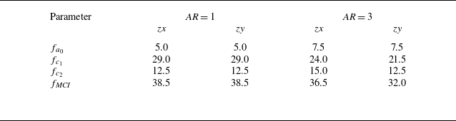
In the following analysis, the zero-, first- and second-order Fourier coefficients, which characterise the bubble size, eccentricity and primary deformation, respectively, are investigated. Additionally, the morphological complexity index (
 $\textit{MCI}$
) proposed by Brezina & Pallotti (Reference Brezina and Pallotti2019) is calculated using (3.18) and (3.19) to quantify overall shape complexity. For the individual coefficients, the amplitude
 $c_n$
is obtained via (3.20). To determine the optimal mode truncation order
 $n_0$
for the
 $\textit{MCI}$
, a sensitivity study was conducted. As shown in figure 11, the
 $\textit{MCI}$
value stabilises for
 $n_0 \geqslant 3$
, indicating that the additional contributions from higher-order modes (describing finer interfacial details) become negligible for both AR = 1 and AR = 3 bubbles. Consequently,
 $n_0 = 3$
is selected as a robust compromise: it is sufficient to capture the dominant shape components while minimising the influence of minor high-order fluctuations,
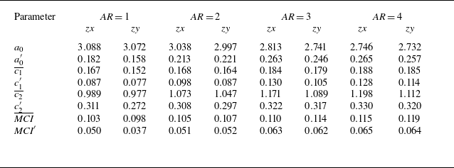
Statistical results of the Fourier coefficients.

Variation of
 $\textit{MCI}$
with the truncation order: (a–b) circular orifice (AR = 1); (c–d) elliptical orifice (AR = 3). Here (a,c)
 ${\textit{zx}}$
plane; (b,d)
 ${\textit{zy}}$
plane.

 \begin{align} E_n &=\frac {1}{2}\left (a_n^2+b_n^2\right ), \end{align}
 \begin{align} {\textit{MCI}} &=1-\frac {\sum _{k=1}^{n_0}E_k}{\sum _{k=1}^{N}E_k}, \end{align}
 \begin{align} c_n &=\sqrt {a_n^2+b_n^2}. \end{align}
Table 3 presents the statistical results of the Fourier coefficients, where overbars denote mean values and primes denote standard deviations. For each tested case, the reported statistics were computed in a framewise manner from a continuous shadowgraphy recording (21 791 frames acquired at 1000 Hz, corresponding to a sampling duration of approximately 21.8 s), with each frame treated as one sample. The recording contains an ensemble of multiple bubbles (
 $O(10^2)$
bubbles per case), based on the measured generation frequency shown in figure 7. The size parameter
 $a_0$
indicates that the bubbles generated by the circular orifice had a larger mean diameter than those generated by the elliptical orifice, which agrees with figure 3. Moreover, the statistics obtained via the 2-D Fourier method closely matched those obtained from the 3-D reconstruction described in Appendix A, confirming the validity of the experimental approach. The greater standard deviation
 $a_0^\prime$
for the elliptical orifice can be explained by the Laplace–Young equation; size variations during ascent occur primarily owing to pressure changes resulting from the height of the bubble (de Gennes, Brochard-Wyart & Quéré Reference de Gennes, Brochard-Wyart and Quéré2004). Because both orifice geometries shared the same experimental environment, the greater
 $a_0^\prime$
for the elliptical case likely reflects the limitations of 2-D analysis. As bubbles ascend, they become non-spherical and rotate about all three axes; therefore, a constant diameter cannot be expected from 2-D measurements (Bröder & Sommerfeld Reference Bröder and Sommerfeld2007; Masuk, Salibindla & Ni Reference Masuk, Salibindla and Ni2019). The increase in variance indicates a stronger dimensionality in 3-D in the bubble motion for the elliptical orifice. Similarly, both the mean values and standard deviations of the centroid offset parameter
 $c_1$
, primary deformation parameter
 $c_2$
and
 $\textit{MCI}$
were greater for the elliptical orifice than for the circular orifice, demonstrating that bubbles from the elliptical orifice underwent more pronounced deformation during ascent.
Bubbles generated from (a–c) a circular orifice (AR = 1) and (d–f) an elliptical orifice (AR = 3). Panels (a) and (d) present the variation in the
 $\textit{MCI}$
along the height, subpanels (i) show the instantaneous bubble shapes in the
 ${\textit{zx}}$
plane and (ii) show the instantaneous bubble shapes in the
 ${\textit{zy}}$
plane.

The instantaneous bubble morphology was examined for two cases: bubbles issued from a circular orifice and bubbles issued from an elliptical orifice with an AR = 3. The variation in the
 $\textit{MCI}$
along the vertical direction is shown in figure 12, where the dimensionless height is defined as
 $z/D_n$
. For bubbles generated from the circular orifice, the
 $\textit{MCI}$
values in the
 ${\textit{zx}}$
(major axis) and
 ${\textit{zy}}$
(minor axis) planes exhibit only slight differences and fluctuate within a narrow range of 0.05–0.15. A distinct increase in
 $\textit{MCI}$
appears when
 $z/D_n$
reaches approximately 5–10, indicating a rapid growth in bubble shape complexity. This transition corresponds to an intensified deformation and pronounced oscillations on both sides of the bubble, as demonstrated by the instantaneous contours in figure 12. In contrast, bubbles from the elliptical orifice display a clear discrepancy in the
 $\textit{MCI}$
between the
 ${\textit{zx}}$
and
 ${\textit{zy}}$
planes. High shape complexity was evident immediately after detachment, which is consistent with the asymmetric surface tension distribution inferred from the contact angle analysis. This suggests that non-uniform interfacial tension during the formation process induces substantial initial deformation. As
 $z/D_n$
increased to approximately 5–10, the
 $\textit{MCI}$
in the
 ${\textit{zx}}$
plane became significantly larger than that in the
 ${\textit{zy}}$
plane. The corresponding bubble shapes revealed a larger projected area in the
 ${\textit{zx}}$
plane, contributing to a more complex morphology compared with the
 ${\textit{zy}}$
plane.
Figure 13 shows the evolution of the Fourier coefficients with respect to
 $z/D_n$
. For the circular orifice, the coefficients in the
 ${\textit{zx}}$
and
 ${\textit{zy}}$
planes remain nearly identical near the orifice but start to diverge when
 $z/D_n$
exceeds 15. Despite this divergence, the overall morphological development is mostly synchronous between the two planes. The onset of the deviation is likely caused by alternating shedding of wake vortices, which modifies the surrounding flow field (Aoyama et al. Reference Aoyama, Hayashi, Hosokawa and Tomiyama2016; Wang et al. Reference Wang, Xu, Li and Wang2024). For the elliptical orifice, pronounced differences between the two planes emerged immediately after detachment, peaking within
 $z/D_n$
= 5–10. This is consistent with the contact angle variations discussed in § 3.1.1. The initial disparity in contact angles along the major and minor axes resulted in an uneven surface tension distribution, which in turn led to a rapid divergence in the bubble contours projected onto the
 ${\textit{zx}}$
and
 ${\textit{zy}}$
planes.
Variation in Fourier coefficients with height: (a–b) zero-order coefficient
 $a_0$
, (c–d) first-order coefficient
 $c_1$
and (e–f) second-order coefficient
 $c_2$
. Here (a,c,e) circular orifice (AR = 1); (b,d, f) elliptical orifice (AR = 3).

The Lomb–Scargle periodogram was employed for the spectral characterisation of several Fourier parameters (VanderPlas Reference VanderPlas2018). The choice of this method reflects our procedure of computing and averaging the spectrum for each individual bubble ascent rather than performing a single analysis on the entire time series, in which case the dominant peak is contaminated by the bubble generation frequency. The Lomb–Scargle method is a least squares-based spectral estimator that is especially well suited to non-uniform and irregularly sampled data and thus ideal for cases in which the ascent period of each bubble differs. The governing equations are expressed in (3.21)–(3.26), where
 $\omega =2\pi f$
.
First, the bubble-shaped signal (
 $s_b$
) is modelled as a linear combination of the cosine and sine functions:
 \begin{equation} s_b\left (t_i\right )=A\cos {\omega t_i}+B\sin {\omega t_i}+\varepsilon _i. \end{equation}
To remove the phase bias introduced by uneven sampling, frequency-dependent time
 $\tau (\omega )$
is defined so that the cosine and sine basis functions become orthogonal in a statistical sense. The shift is computed as
 \begin{equation} \tan \left (2\omega \tau \right ) = \frac {\sum _{i=1}^{n} \sin \left (2\omega t_i\right )}{\sum _{i=1}^{n} \cos \left (2\omega t_i\right )}. \end{equation}
The shifted basis functions are then
 \begin{equation} C_i = \cos \left [\omega \left (t_i - \tau \right )\right ], \quad S_i = \sin \left [\omega \left (t_i - \tau \right )\right ]. \end{equation}
By minimising the residual sum of squares, (3.24) yields the coefficients
 $A$
and
 $B$
as expressed in (3.25), and the corresponding power spectral density (
 $\textit{PSD}$
) is given by (3.26), where
 \begin{align} & \sum \big [s_b\left (t_i\right ) -AC_i-BS_i\big ]^2, \end{align}
 \begin{align} A &=\frac {\sum _{i}{s_b\left (t_i\right )C_i}}{\sum _{i} C_i^2}, \quad B=\frac {\sum _{i}{s_b\left (t_i\right )S_i}}{\sum _{i} S_i^2}, \end{align}
 \begin{align} & {\textit{PSD}} \left (\omega \right ) =\frac {1}{2}\Big (A^2+B^2\Big ). \end{align}
The dominant frequencies of each parameter are listed in table 4. An analysis of the full time series revealed that for the circular orifice, the Fourier coefficients exhibited similar periodic behaviour in both the
 ${\textit{zx}}$
and
 ${\textit{zy}}$
planes. In contrast, for the elliptical orifice, the periodic characteristics for the two directions differed significantly. This indicates that, in the case of the circular orifice, both the deformation and size variations during ascent are approximately isotropic across the two planes, likely owing to bubble-induced wake dynamics (Bonnefis et al. Reference Bonnefis, Fabre and Magnaudet2023). Conversely, the initial geometric asymmetry of the elliptical orifice resulted in pronounced directional discrepancies. A detailed discussion incorporating the flow field results is provided in § 3.3.1.
Dominant frequencies of Fourier coefficients.

Bubble trajectories during rising: (a–b) circular orifice (AR = 1), (c–d) elliptical orifice (AR = 2), (e–f) elliptical orifice (AR = 3) and (g–h) elliptical orifice (AR = 4). Here (a,c,e,g) 3-D trajectories; (b,d, f,h) projections onto the
 $xy$
plane.

3.2. Bubble kinematics
3.2.1. Bubble motion
Figure 14 shows the trajectories of the bubbles during the rising process. Regardless of the orifice geometry, the bubbles initially undergo a rectilinear rise, followed by a transition into an oscillating rise. For bubbles generated from the circular orifice, the trajectory resembles a spiral path due to the approximately equal displacements along the major and minor axes. In contrast, bubbles from an elliptical orifice exhibit a zigzag trajectory, with the displacement along the minor axis significantly exceeding that along the major axis (Wu & Gharib Reference Wu and Gharib2002; Veldhuis et al. Reference Veldhuis, Biesheuvel and Wijngaarden2008). This directional asymmetry is consistent with the morphological analysis presented in § 3.1.3.
Schematic illustration of the calculation of the geometric polar moment of inertia
 $J_c$
for a bubble cross-section: (a) zx plane; (b) zy plane.

Variation of moment of inertia with height: (a) circular orifice (AR = 1); (b) elliptical orifice (AR = 3).

The geometric second moments of area for each bubble cross-section were calculated using (3.27) and (3.28), as schematically shown in figure 15. The corresponding evolution of these moments for the circular (AR = 1) and elliptical (AR = 3) orifices is presented in figure 16. Results indicate that the moments of inertia for the circular orifice remain nearly identical in both directions. However, the elliptical orifice exhibits significant anisotropy near the region where the bubble deviates from a rectilinear rise. Specifically, the moment associated with the
 ${\textit{zx}}$
-plane is notably larger than that of the
 ${\textit{zy}}$
-plane, with approximately
 $J_{c,zx} \approx 2J_{c,zy}$
observed in the deviation-onset region:
 \begin{align} J_{c,zx} &= \iint _A \left [(x - x_c)^2 + (z - z_c)^2 \right ] {\textrm d}A, \end{align}
 \begin{align} J_{c,zy} &= \iint _A \left [(y - y_c)^2 + (z - z_c)^2 \right ] {\textrm d}A. \end{align}
At the instability height – marking the transition from rectilinear to oscillating rise – the projection of the entire bubble volume onto the
 ${\textit{zx}}$
-plane is larger than that onto the
 ${\textit{zy}}$
-plane. Additionally, the moment of inertia of the bubble about the axis normal to the
 ${\textit{zy}}$
-plane is smaller. These differences make the bubble more susceptible to rotational deviation towards the minor-axis direction when disturbed by the surrounding flow, resulting in a greater displacement in that direction. Moreover, bubbles generated from a circular orifice typically become unstable at a higher height than those from an elliptical orifice. This agrees with the morphological characteristics discussed in § 3.1.3: bubbles from a circular orifice are approximately isotropic, whereas bubbles from an elliptical orifice exhibit clear anisotropy. Higher shape symmetry tends to slow the growth of initial disturbances, so the transition from rectilinear rise to oscillatory rise is delayed under the circular-orifice condition and tends to occur at a greater height. In contrast, the more complex deformation of bubbles from an elliptical orifice is more likely to induce a complex wake, leading to path instability (Duineveld Reference Duineveld1995; Wang et al. Reference Wang, Xu, Li and Wang2024). A detailed flow field analysis is presented in § 3.3.1.
Variation in bubble diameter and rising velocity with height: (a) equivalent diameter
 $d_b$
; (b) rising velocity
 $V_b$
.

In addition to trajectory statistics, the bubble terminal rising velocity and the associated dimensionless groups are analysed. Figure 17 shows the variation of the terminal rising velocity with height, together with the corresponding equivalent diameter used to evaluate the dimensionless parameters. The equivalent diameter
 $d_b$
exhibits pronounced volume oscillations for
 $z/D_n \leqslant 10$
, consistent with the near-orifice acceleration stage. This behaviour is attributed to the acceleration region immediately after detachment, where inertial effects can cause transient bubble compression followed by relaxation (Lee & Park Reference Lee and Park2022; Wang et al. Reference Wang, Xu, Li and Wang2024). Under the present conditions, the bubbles enter a quasisteady rising regime for
 $z/D_n\geqslant 15$
, in which the rising velocity becomes approximately constant.
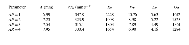
The statistics indicate that, as the orifice AR increases from 1 to 4, the equivalent diameter decreases from 6.39 to 5.25 mm, while the terminal rising velocity decreases from 347.8 mm s−1 to 300.4 mm s−1. Overall, bubbles released from the circular orifice exhibit higher terminal velocities than those released from elliptical orifices, consistent with their larger size and a buoyancy–drag balance in which the terminal velocity increases with bubble size (Wang et al. Reference Wang, Xu and Li2025a ).
The dimensionless numbers are defined in (3.29)–(3.32), and the statistical results are summarised in table 5. In these definitions,
 $\textit{VT}_b$
is the bubble terminal rising velocity,
 $\rho _l$
and
 $\rho _g$
are the liquid and gas densities, respectively,
 $\nu$
is the kinematic viscosity of the liquid,
 $\mu _l$
is the dynamic viscosity of the liquid,
 $\sigma$
is the surface tension, and
 $g$
is the gravitational acceleration. The decrease of
 ${\textit{Re}}$
,
 ${\textit{We}}$
,
 ${\textit{Eo}}$
and
 ${\textit{Ga}}$
with increasing AR indicates that, relative to the elliptical-orifice cases, inertial effects are more pronounced for the circular-orifice case, whereas surface tension plays a comparatively stronger role for the elliptical-orifice cases. Following Yang, Prosperetti & Takagi (Reference Yang, Prosperetti and Takagi2003) and Mei & Cheng (Reference Mei and Cheng2022), even the largest
 ${\textit{Eo}}$
in the present study remains within a moderate-
 ${\textit{Eo}}$
regime, in which surface tension continues to influence deformation through interfacial-energy relaxation that suppresses excessive shape distortion. These observations suggest that the bubbles undergo time-dependent deformation during ascent; the role of dimensionless groups in trajectory deviation is therefore examined with particular emphasis on the Eötvös number
 ${\textit{Eo}}$
and the Weber number
 ${\textit{We}}$
:
 \begin{align} {\textit{Re}} &= \frac {{\textit{VT}}_b{d}_{b}}{\mathrm{\nu }}, \end{align}
 \begin{align} {\textit{We}} &= \frac {\rho_l {\textit{VT}}_b^2{d}_{b}}{\mathrm{\sigma }}, \end{align}
 \begin{align} {\textit{Eo}} &= \frac {g (\rho _l-\rho _g)d_b^2}{\sigma }, \end{align}
 \begin{align} {\textit{Ga}} &= \frac {(\rho _l-\rho _g)^{\frac {1}{2}}\rho _l^{\frac {1}{2}}g^{\frac {1}{2}}d_{b}^{\frac {3}{2}}}{\mu _l}. \end{align}
The relative importance of surface tension, buoyancy and inertia is commonly characterised using
 ${\textit{Eo}}$
and
 ${\textit{We}}$
. Previous studies show that larger
 ${\textit{Eo}}$
tends to promote stronger deformation and wake asymmetry, which can lead to lateral trajectory oscillations (Bonnefis et al. Reference Bonnefis, Sierra-Ausin, Fabre and Magnaudet2024). Larger
 ${\textit{We}}$
tends to strengthen shape oscillations and interfacial instability (Duineveld Reference Duineveld1997). Therefore, if classical size effects were the main cause, then increasing AR (which reduces
 $d_b$
in the present experiments and thus reduces
 ${\textit{Eo}}$
and
 ${\textit{We}}$
) should make the path more stable: the instability onset should occur later (at a higher onset height), and the oscillation amplitude should decrease.
Statistical results of dimensionless parameters.

However, the measured trend is opposite. When
 $\textit{AR}$
increases from 1 to 4, the non-dimensional onset height
 $z/D_n$
decreases from 5.3 to 4.5, and the oscillation amplitude increases from 6.99 to 7.95. This trend is opposite to the
 ${\textit{Eo}}$
-
 ${\textit{We}}$
based expectation from classical size effects, indicating that classical size effects alone cannot explain the observed results.
This behaviour is consistent with the geometry-specific effect. With larger AR, the bubble shape at formation becomes more anisotropic and less symmetric. This makes wake asymmetry easier to develop and can trigger lateral motion earlier. In other words, as AR increases, the geometry-specific effect becomes stronger and can dominate the path behaviour, even though classical size effects at smaller
 ${\textit{Eo}}$
/
 ${\textit{We}}$
would suggest more stability.
To make this point more quantitative, we introduce a
 $\textit{MCI}$
in § 3.1.3 to describe how strong and how complex the geometry-related shape perturbations are. A larger
 $\textit{MCI}$
means stronger and more complex shape perturbations, which usually come with a more unsteady path. We then propose a composite stability index
 ${\textit{SI}}$
that includes
 ${\textit{Eo}}$
,
 ${\textit{We}}$
and
 ${\textit{MCI}}$
, and relate the oscillation amplitude
 $A$
to
 ${\textit{SI}}$
,
 \begin{align} {\textit{SI}} &= \frac {1}{{\textit{Eo}}^{c}\,{\textit{We}}^{d}\,{\textit{MCI}}^{e}}, \end{align}
 \begin{align} A &= k\,SI^{-1}, \end{align}
which is equivalent to the power-law form
 $A=k\,{\textit{Eo}}^{c}{\textit{We}}^{d}{\textit{MCI}}^{e}$
. The coefficients are obtained by performing a regression in log space, i.e. fitting
 $\ln A=\ln k+c\ln Eo+d\ln We+e\ln \textit{MCI}$
using a bound-constrained nonlinear least-squares solver, with the exponents constrained to be non-negative
 $(c,d,e\ge 0)$
to enforce physically expected monotonic trends (Coleman & Li Reference Coleman and Li1996). A weak Tikhonov regularisation term is included to keep the exponents within physically reasonable ranges. The coefficient of determination
 $R^2$
is evaluated in the original
 $A$
-space using the fitted values of
 $A$
. For the present dataset, the fitting yields
 $k=7.46$
,
 $c=0.28$
,
 $d=1.05$
and
 $e=1.34$
, with
 $R^2=0.92$
. For comparison, fitting results excluding
 ${\textit{MCI}}$
are also reported. As shown in figure 18, the fit including
 ${\textit{MCI}}$
captures the change of
 $A$
, while a fit using only
 ${\textit{Eo}}$
and
 ${\textit{We}}$
is almost flat and does not reproduce the trend. This ratio-type form has also been used in dimensionless correlations in the literature (Aoyama et al. Reference Aoyama, Hayashi, Hosokawa and Tomiyama2016). These results show that
 ${\textit{Eo}}$
and
 ${\textit{We}}$
alone cannot reproduce the observed trend; adding
 ${\textit{MCI}}$
is necessary, which indicates that the geometry-specific effect is the main cause of the earlier onset and larger oscillations in our experiment.
Trajectory oscillation amplitude
 $A$
for different orifice ARs.

3.2.2. Force analysis of the rising bubble
To further investigate the dynamics of bubble motion, the force-budget framework employed in this study is summarised. The force diagram is presented in figure 19, and the corresponding expressions for the forces are given in (3.35)–(3.39). Along the rise direction (
 $z$
-direction), the relevant forces include buoyancy
 $F_B$
, drag
 $F_{\textit{Dz}}$
, wake-induced suction
 $F_w$
from a preceding bubble, the rotation-related term
 $F_{\varOmega z}$
(Mougin & Magnaudet Reference Mougin and Magnaudet2002, Reference Mougin and Magnaudet2003) and the inertial force
 $F_{\textit{Iz}}$
. The inertial force represents the response of the surrounding liquid set into motion by the bubble and acts opposite to the bubble’s motion relative to the liquid. Following Kim et al. (Reference Kim, Kamotani and Ostrach1994), the inertial force is decomposed into
 $F_{\textit{Imz}}$
, associated with bubble-volume (mass) variations, and
 $F_{\textit{Ivz}}$
, associated with bubble-velocity variations. In the lateral directions (
 $x$
and
 $y$
), the deviation dynamics are mainly governed by the competition between the rotation-induced forces
 $F_{\varOmega x}$
(or
 $F_{\varOmega y}$
) and the combined contributions of drag and inertial forces in the same direction, namely
 $F_{\textit{Dx}}$
together with
 $F_{\textit{Ix}}$
(or
 $F_{\textit{Dy}}$
together with
 $F_{Iy}$
). The forces are expressed as follows:
 \begin{align} F_B &= {Vol}_b (\rho _l - \rho _g) g, \end{align}
 \begin{align} F_W &= C_{i,i-1} \frac {1}{2} \rho _l V_{\textit{eff}}^2 A_{\textit{eff}}, \end{align}
 \begin{align} F_{\varOmega } &= (\rho _g + C_M \rho _l) Vol_b \boldsymbol{\cdot }\varOmega \times V_{\textit{eff}}, \end{align}
 \begin{align} F_D &= C_D \frac {1}{2} \rho _l V_{\textit{eff}}^2 A_{\textit{eff}}, \end{align}
 \begin{align} F_I = F_{\textit{Im}} + F_{\textit{Iv}} = \frac {{\textrm d}M}{{\textrm d}t} V_{\textit{eff}} & + M \left (\frac {{\textrm d}V_{\textit{eff}}}{{\textrm d}t}\right ) = \left (\frac {d((\rho _g + C_M \rho _l) Vol_b)}{{\textrm d}t}\right ) V_{\textit{eff}} \nonumber\\ &\quad +\, (\rho _g + C_M \rho _l) Vol_b \left (\frac {{\textrm d}V_{\textit{eff}}}{{\textrm d}t}\right ), \end{align}
Force balance during the bubble rising stage. The directions of
 $F_{\varOmega }$
,
 $F_D$
and
 $F_I$
are valid only for the rotation and translational directions illustrated here; when the bubble undergoes lateral deflection, the directions of these forces may change accordingly.

where
 $\rho _g$
is the gas density inside the bubble,
 $g$
is the gravitational acceleration,
 ${Vol}_b$
is the bubble volume,
 $V_{\textit{eff}}$
is the relative velocity in the corresponding direction,
 $A_{\textit{eff}}$
is the projected area of the bubble in that direction,
 $M$
is the effective mass, including the bubble mass and the mass of the surrounding fluid set into motion by the bubble translation and
 $\varOmega$
is the angular velocity of the bubble. The coefficients associated with these forces are evaluated using (3.40) (Rastello, Marié & Lance Reference Rastello, Marié and Lance2011), (3.41) (Karamanev Reference Karamanev1994), and (3.42) (Harper Reference Harper1970):
 \begin{align} &C_m = \frac {\gamma _0}{2 - \gamma _0}, \quad \gamma _0 = \frac {2}{e^2} \left (1 - \sqrt {1 - e^2} \frac {\arcsin (e)}{e}\right ), \quad e = \sqrt {\frac {\chi ^2 - 1}{\chi }}, \end{align}
 \begin{align} &\qquad \qquad \quad C_d = \frac {24(1 + 0.173 Re^{0.657})}{Re} + \frac {0.413}{1 + 16300 Re^{-1.09}}, \end{align}
 \begin{align} & \qquad \qquad \qquad \qquad \qquad \qquad C_{i,i-1} \approx 12 s^{-4}, \end{align}
where
 $\chi$
denotes the bubble AR,
 ${\textit{Re}}$
is the Reynolds number and
 $s$
is the interbubble spacing.
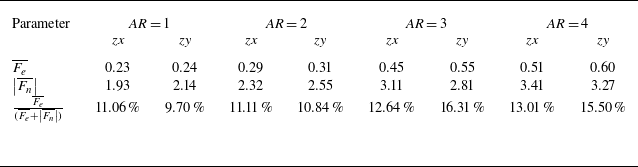
The force-budget analysis in figure 20 indicates that, along the rise direction, the dominant balance is between buoyancy
 $F_B$
and the vertical drag
 $F_{\textit{Dz}}$
. In the present spacing range, the wake-induced suction force
 $F_W$
is found to be small and is not a leading term in the mean vertical balance. Consequently, buoyancy is slightly larger than drag, providing the net force required by the observed rise motion and the inertial response induced by shape oscillations. In the
 $z$
-direction, the inertial contribution induced by bubble mass (shape) oscillations (
 $F_{\textit{Imz}}$
) is larger than that associated with variations of the bubble rise velocity (
 $F_{\textit{Ivz}}$
). In the lateral directions (
 $x$
and
 $y$
), the deviation dynamics are governed by the competition between
 $F_\varOmega$
and
 $F_{\textit{Iv}}$
. This framework aligns with Mougin & Magnaudet (Reference Mougin and Magnaudet2002, Reference Mougin and Magnaudet2003), who demonstrated that path instability results from the coupling between wake vorticity and hydrodynamic forces (specifically torque and rotation-induced force), and Shi, Zhang & Magnaudet (Reference Shi, Zhang and Magnaudet2024), who emphasised the feedback of shape-induced inertia on translational dynamics. However, the orifice AR critically alters this force balance through two distinct mechanisms. First, the anisotropy of the rotation-induced force (
 $F_{\varOmega y} \gt F_{\varOmega x}$
) becomes significant due to the larger oscillation amplitude along the minor axis. This disparity breaks the lateral symmetry required for a stable spiral, thereby favouring a planar-like motion. Second, the destabilising inertial force (
 $F_{\textit{Iv}}$
) significantly increases and eventually surpasses
 $F_\varOmega$
. This enhancement arises because, even though the mean wake suction (
 $F_W$
) is small, the wake imposes disturbances that amplify the velocity pulsations of the trailing bubble (Hessenkemper et al. Reference Hessenkemper, Bragg, Lucas and Ma2025). Consequently, the observed zigzag trajectory is driven by the combined effect of force anisotropy (
 $F_{\varOmega y} \gt F_{\varOmega x}$
) breaking the spiral symmetry and inertial dominance (
 $F_{\textit{Iv}} \gt F_\varOmega$
) enforcing the instability.
Mean force components during the bubble rising stage: (a)
 $F_x$
; (b)
 $F_y$
; (c)
 $F_z$
.

This force analysis offers a baseline for understanding multibubble systems, such as bubble columns and airlift reactors (Mahmood et al. Reference Mahmood, Abdulrahman, Sabri, Sultan, Majdi and Al-Dahhan2024). The connection depends on how orifice geometry shifts the relative importance of key forces. Specifically, increasing the orifice
 $AR$
modifies bubble morphology, rise velocity and rotation, which directly changes the drag (
 $F_D$
) and rotation-induced forces (
 $F_{\varOmega }$
). Furthermore, it alters the velocity pulsations and the local turbulence described in § 3.4.3, thereby affecting the inertial force associated with velocity variations (
 $F_{\textit{Iv}}$
). In multibubble configurations, these effects are amplified because wake disturbances and BIT are naturally stronger (Hessenkemper et al. Reference Hessenkemper, Bragg, Lucas and Ma2025), while wake interactions can modify the rise path (Legendre, Magnaudet & Mougin Reference Legendre, Magnaudet and Mougin2003). External flow and shear may also influence the initial formation and lateral drift (Mirsandi et al. Reference Mirsandi, Smit, Kong, Baltussen, Peters and Kuipers2020). Ultimately, the trend identified here is expected to persist in denser systems: as the
 $AR$
increases, the rotation force weakens while the inertial force becomes dominant. This effect is likely to be even more pronounced in dense bubble swarms, consistent with Xu et al. (Reference Xu, Tan, Qi and Ni2025), who showed that bubble deformation directly enhances BIT.
3.3. Bubble-induced flow field
Prior to the velocity field analysis, the uncertainty in the instantaneous velocity was assessed. According to the error propagation formula proposed by Kline & McClintock (Reference Kline and McClintock1953), the uncertainty in velocity (
 $\varepsilon _v$
) originates from the uncertainties in displacement (
 $\varepsilon _x$
) and time (
 $\varepsilon _t$
). Because
 $\varepsilon _t$
is negligible (Qu et al. Reference Qu, Wang, Feng and He2019), the uncertainty in velocity can be approximated as
 \begin{equation} \varepsilon _v=\sqrt {\left (\frac {\partial v}{\partial x}\right )^2\varepsilon _x^2+\left (\frac {\partial v}{\partial t}\right )^2\varepsilon _t^2}=\varepsilon _xf, \end{equation}
where f denotes the particle image acquisition frequency. By substituting the displacement uncertainties from FOV1 and FOV2, as defined in § 2, the calculated velocity uncertainties were
 $\varepsilon _{v1}$
= 7.4 mm s−1 and
 $\varepsilon _{v2}$
= 4.9 mm s−1. The relative uncertainty, normalised by the terminal velocity of the bubble, was approximately 2.1 %–2.3 % for FOV1 and 1.4 %–1.5 % for FOV2.
The uncertainty in the experimental vorticity was also evaluated. Vorticity calculations involve spatial differentiation, which potentially may introduce errors. Based on research by Sciacchitano & Wieneke (Reference Sciacchitano and Wieneke2016), the vorticity uncertainty was estimated using (3.44), where
 $d_w$
is the vector pitch, and
 $c_{xx}$
is the velocity cross-correlation coefficient between two spatial points separated by
 $2d_w$
. When the interrogation window size was set to 32
 $\times$
32 pixels with 75 % overlap,
 $c_{xx}$
was approximately 0.45 (Sciacchitano & Wieneke Reference Sciacchitano and Wieneke2016). The estimated vorticity uncertainty (
 $\varepsilon _\omega$
) was approximately 6.2
 $\textrm {s}^{-1}$
and remained consistent across both FOVs. The corresponding relative uncertainty, calculated by normalising
 $\varepsilon _\omega$
with a characteristic vorticity scale based on the bubble velocity and orifice diameter, ranged from 7.0 %–7.8 %. These results confirm that the vorticity measurements in this study have high reliability and acceptable accuracy,
 \begin{equation} \varepsilon _\omega =\frac {\varepsilon _v}{d_w}\sqrt {1-c_{xx}}. \end{equation}
To quantify the flow strength, the local time-averaged velocity magnitude is first derived from the instantaneous radial (
 $u$
) and vertical (
 $v$
) components. Based on these profiles, the wake half-width was identified as the radial location where the velocity decays to the midpoint between the centreline peak and the background level. For the results presented in figure 21, the velocity magnitude
 $|\overline {U}|$
is calculated by spatially averaging the time-mean profile within this half-width region at each height. The results demonstrate that while the velocity stabilises beyond
 $z/D_n \approx 20$
, the stable values do not merge into a single curve. The flow velocity remains systematically lower for higher AR cases; specifically, as AR increases from 1 to 4, the stabilised velocity decreases from 118.9 mm s−1 to 82.3 mm s−1. Within the extended observation window, there is no sign of the flow fields from different geometries converging. Thus, the influence of the orifice geometry persists because it sets the initial bubble size and deformation, which in turn determines the rising velocity and the flow field intensity.
Variation of the half-width average velocity with height.

3.3.1. Evolution of instantaneous flow field
As previously established, when the elliptical orifice AR
 $\geqslant$
3, the bubble morphology and kinematics undergo marked changes. Accordingly, this section focuses on two cases of induced flow field, namely, a circular orifice and an elliptical orifice with AR = 3. Because the
 ${\textit{zx}}$
and
 ${\textit{zy}}$
planes were not recorded simultaneously, representative time instants during bubble ascent were selected to compare the instantaneous flow structures across the two planes. Clear differences emerged between the flows induced by bubbles from the circular and elliptical orifices. Figure 22 shows the case involving the circular orifice. Rising bubbles typically generated a pair of large-scale counter-rotating wake vortices resulting from regular vortex shedding in their wake. This pattern was promoted by the relatively uniform shape of the bubble and near-axisymmetric surface tension distribution imparted by the circular orifice. Consequently, the bubbles maintained stable periodic path oscillations during ascent, enabling a coherent roll-up of the shear layers into organised vortex pairs. These observations are consistent with the classical descriptions of single bubble wake structures (Cao & Macián-Juan Reference Cao and Macián-Juan2021).
Instantaneous flow fields induced by bubbles from a circular orifice (AR = 1): (a)
 ${\textit{zx}}$
plane flow field; (b)
 ${\textit{zy}}$
plane flow field.

In contrast, the flow structures induced by the bubbles from the elliptical orifice, as shown in figure 23, reflect a pronounced initial shape asymmetry. As discussed in § 3.1.1, an asymmetric contact angle during bubble formation leads to an uneven surface tension distribution during detachment. This asymmetry initiates strong 3-D deformations of the bubble surface early in the rising process, enhancing path instability and significantly disrupting wake development. Rather than forming a stable, large-scale vortex pair, the shear layers continuously generate and release multiple small-scale vortices. These vortices interact, merge and evolve into a wake structure characterised by reduced coherence, enhanced velocity fluctuations and spatial asymmetry.
Instantaneous flow fields induced by bubbles from an elliptical orifice (AR = 3): (a)
 ${\textit{zx}}$
plane flow field; (b)
 ${\textit{zy}}$
plane flow field.

To further elucidate the coupling relationship between the flow field structures and bubble dynamics, Fourier mode decomposition (FMD) was employed to analyse the flow field in the frequency domain (Ma et al. Reference Ma, Feng, Pan, Gao and Wang2015; He et al. Reference He, Guo, Xu, Feng and Wang2023), as shown in figure 24. The discrete Fourier transform at each spatial grid point (
 $x_i$
,
 $y_i$
) was defined by (3.45), where
 $N_{\textit{image}}$
denotes the total number of sampled image pairs,
 $t_n$
is the sampling time of the
 $n_th$
image pair,
 $f_k$
is the target frequency and
 $F$
represents the complex-valued velocity data. The average of the complex modal components within the frequency band
 $[f_0-\Delta f,f_0+\Delta f]$
was calculated using (3.46), where
 $\Delta f$
was set to 1 Hz in this study to represent the dominant modal response. The time-dependent velocity field at the dominant frequency was reconstructed using (3.47), where the phase distribution
 $\varphi (x,y)$
is defined as
 $\varphi (x,y )=\arctan ({{v(x,y)}/{u(x,y)}})$
:
 \begin{align} \hat {U} (x_i,y_j,f_k) &=\sum _{n=0}^{N_{\textit{image}}-1}F (x_i,y_j,t_n)\boldsymbol{\cdot }e^{-i2\pi f_kt_n}, \end{align}
 \begin{align} \hat {U}_{\textit{mode}}(x,y) &= \frac {1}{N_f} \sum _{f \in [f_0-\Delta f, f_0+\Delta f]} \hat {U}(x,y,f), \end{align}
 \begin{align} F_{f_0}\left (x,y,t\right ) &=2\boldsymbol{\cdot }\big |{\hat {U}}_{\textit{mode}}\left (x,y\right )\big |\boldsymbol{\cdot }\cos {\left (2\pi f_0t+\varphi \left (x,y\right )\right )}. \end{align}
Vorticity fields reconstructed using FMD: (a)
 ${\textit{zx}}$
plane for the circular orifice (AR = 1); (b)
 ${\textit{zx}}$
plane for the elliptical orifice (AR = 3); (c)
 ${\textit{zy}}$
plane for the elliptical orifice (AR = 3).

A FMD analysis was conducted to identify the flow field structures corresponding to the dominant frequencies of each bubble parameter described in § 3.1.3, as shown in figure 24. The frequencies used to extract the wake structures in figure 24 are the same dominant-frequency values reported in table 4. Given the previously validated similarity between the induced flow fields of the bubbles generated by the circular orifices and the consistent dominant frequencies of the bubble parameters, decomposition was performed on a representative plane (
 ${\textit{zx}}$
) for the circular orifice only. The results indicated that the flow structure corresponding to the dominant frequency of the size parameter
 $a_0$
exhibited the strongest modal amplitude. The induced flow structures for the circular orifice at this frequency were larger than those associated with the elliptical orifice. The deformation parameter
 $c_2$
corresponded to a relatively large-scale structure. In contrast, the modes associated with
 $c_1$
and
 $\textit{MCI}$
were dominated by small-scale structures, suggesting that bubble-induced flow disturbances were primarily governed by the overall size and principal deformation of the bubbles, whereas high-frequency oscillations of the bubble geometry led to more localised, small-scale features. Furthermore, at higher frequencies, the flow structures induced by elliptical orifices exhibited distinct spatial distributions in different planes: in the
 ${\textit{zx}}$
plane, the dominant structures were concentrated near the orifice region (
 $z/D_n \approx 5-10$
), whereas in the
 ${\textit{zy}}$
plane, the structures were predominantly located in the upper regions where surface oscillations of the bubble become more pronounced during ascent. This indicates that, in the
 ${\textit{zx}}$
plane, flow is strongly influenced by near-orifice oscillations, whereas in the
 ${\textit{zy}}$
plane, surface-instability-induced deformations during rising play a greater role in shaping flow dynamics.
3.4. Bubble induced turbulence
3.4.1. Analysis of energy spectra in turbulent bubbly flows
Analyses of both the time-averaged and instantaneous flow fields revealed a strong connection between the bubble morphology and flow structures. As the bubbles rose, the induced flow field was observed to became increasingly widespread and structurally complex. To further understand the influence of bubbles on flow turbulence, the turbulent characteristics of the bubble-induced flow field were investigated. As a prerequisite, power spectral analysis was performed. In bubble-induced flows, the velocity power spectra at different vertical positions exhibit distinct trends in both magnitude and spectral slope, reflecting the interplay between bubble dynamics, energy transfer and multiscale flow structures (Prakash et al. Reference Prakash, Mercado, Wijngaarden, Mancilla, Tagawa, Lohse and Sun2016). The energy spectrum method proposed by Lance & Bataille (Reference Lance and Bataille1991) was employed to compute the one-dimensional velocity spectra along the centreline (i.e.
 $x/D_n$
= 0 or
 $y/D_n$
= 0). The spectral calculations were performed at three heights, namely,
 $z/D_n$
= 5, 15 and 25, and the corresponding results are presented in figure 25.
The
 $\textit{PSD}$
of the velocity field in FOV1: (a–b) circular orifice (AR = 1); (c–d) elliptical orifice (AR = 3). Here (a,c)
 ${\textit{zx}}$
plane; (b,d)
 ${\textit{zy}}$
plane.

At a lower height near the orifice (
 $z/D_n$
= 5), the spectrum exhibits pronounced peaks and oscillations at low wavenumbers. This is primarily attributed to the complex gas–liquid interactions occurring near the orifice (Wang et al. Reference Wang, Xu, Li and Wang2024). From the perspective of bubble generation mechanisms, gas is injected into a liquid in the form of a jet, and the competition between detachment forces (such as gas momentum and buoyancy) and attachment forces (such as inertia, drag and surface tension) governs bubble formation (Kulkarni & Joshi Reference Kulkarni and Joshi2005). During continuous gas injection, the inherently unsteady nature of the gas–liquid interaction induces strong disturbances in the flow field. These low-frequency, large-scale disturbances manifest as high-amplitude peaks at low wavenumbers in the energy spectrum (Kottapalli et al. Reference Kottapalli, Hirschberg, Anantharaman, Smeulders, Waterson and Nakiboglu2022). As the wavenumber increases, the energy spectrum gradually exhibits a scaling slope approaching −2. This transition indicates a change in the energy transfer and dissipation mechanisms of the flow. Generally, the spectral slope characterises the energy cascades across different spatial scales. At higher wavenumbers corresponding to smaller scales, viscous dissipation becomes increasingly dominant. In bubble-induced flows, small-scale vortices evolve under the influence of viscous forces, and the energy spectrum follows a power-law scaling with a slope approaching −2. This behaviour suggests that small-scale structures in the bubble wake and shear-induced vortices dissipate energy in line with this scaling, marking the onset of pseudoturbulence (Wang & Socolofsky Reference Wang and Socolofsky2019).
Based on the above analysis, we concluded that the flow field within FOV1 is strongly influenced by bubble generation at the orifice. Significant differences between the
 ${\textit{zx}}$
and
 ${\textit{zy}}$
planes further complicated the analysis of the turbulence interfaces and related phenomena within this region. Therefore, an additional flow field analysis was conducted in the higher region, referred to as FOV2. The corresponding results are shown in figure 26.
The
 $\textit{PSD}$
of the velocity field in FOV2: (a–b) circular orifice (AR = 1), and (c–d) elliptical orifice (AR = 3). Here (a,c)
 ${\textit{zx}}$
plane; (b,d)
 ${\textit{zy}}$
plane.

As bubbles rise to higher vertical positions with
 $z/D_n$
exceeding 40, the spectral slope undergoes a distinct transition. At lower wavenumbers, corresponding to larger spatial scales, the spectral slope follows a flatter scaling law and gradually shifts towards a steeper slope of approximately −2 as the wavenumbers increase, reflecting notable changes in turbulence characteristics. In the regime with larger spatial scales (lower wavenumbers), the energy spectrum no longer adheres to the traditional −5/3 power-law scaling described by Kolmogorov in his theory of homogeneous isotropic turbulence. Instead, the spectral slope displays a flatter scaling behaviour, with a magnitude (absolute value) smaller than −5/3. This deviation from the traditional inertial subrange scaling arises from the dominant influence of large-scale flow structures driven by the dynamics of the bubble chain and buoyancy. The sequential ascent of bubbles in the chain, coupled with the buoyancy-induced recirculation zones around individual bubbles and macroscale flow field modulated by their continuous rise, suppresses the formation of traditional inertial subrange turbulence. These large-scale flow features, characterised by slower, more coherent motion rather than the random energy cascade of isotropic turbulence, led to a more gradual distribution of energy across the larger scales, resulting in a flatter scaling law observed at the lower wavenumbers.
As the wavenumbers increase, moving towards smaller spatial scales, the influence of bubble-specific interactions becomes increasingly pronounced. Velocity deficits in the wake of each rising bubble, oscillatory motions of individual bubbles and local flow disturbances caused by adjacent bubbles in the chain disrupt large-scale coherent flows and alter energy transfer and dissipation mechanisms (Xu et al. Reference Xu, Qi, Zhong, Tan, Wu and Ni2024). These small-scale dynamics are strongly dependent on bubble properties such as size and rising velocity, as well as the local flow environment. Here, viscous dissipation begins to dominate, and the energy spectrum transitions away from the flatter large-scale scaling towards a steeper slope of approximately −2 (Lance & Bataille Reference Lance and Bataille1991; Risso Reference Risso2018), marking the shift from buoyancy-driven macroscale flow to bubble-modulated small-scale turbulence.
3.4.2. Fractal dimension analysis of the TNTI
Based on the preceding analysis, the TNTI analysis in this study focused primarily on the flow field within FOV2. The thresholds for TNTI extraction and subsequent geometric feature analysis were determined using the methodology described in Appendix B. First, the fractal dimensions of the bubble-induced flow fields were examined. The fractal dimension provided a quantitative measure of the spatial complexity of the interface and effectively represented the multiscale characteristics of the structure. The box-counting method is widely used to calculate the fractal dimensions of geometric patterns (De Silva et al. Reference De Silva, Philip, Chauhan, Meneveau and Marusic2013; Mistry, Philip & Dawson Reference Mistry, Philip and Dawson2019; Balamurugan et al. Reference Balamurugan, Rodda, Philip and Mandal2020). As shown in figure 27, this method overlays a 2-D image with square grids having a side length
 $\varDelta _{\textit{box}}$
and counts the number (
 $N$
) of boxes containing the interface. As
 $\varDelta _{\textit{box}}$
decreases,
 $N$
increases, and within a specific scale range, the relationship between these two parameters follows the power-law
 \begin{equation} N\left (\varDelta _{\textit{box}}\right )\propto \varDelta _{\textit{box}}^{-D_2}, \end{equation}
where
 $D_2$
denotes the fractal dimension of the 2-D interface. Taking the logarithms of both sides yields
 \begin{equation} D_2 = \frac {\log {N(\varDelta _{\textit{box}})}}{\log \left (\frac {1}{\varDelta _{\textit{box}}}\right )}. \end{equation}
Schematic of the box-counting method.

A TNTI is inherently a highly convoluted 2-D surface embedded in 3-D space, characterised by a fractal dimension
 $D_3$
. However, this study measured the fractal dimension
 $D_2$
of the intersection between the surface and a 2-D measurement plane. According to the codimensional rule proposed by Mandelbrot (Reference Mandelbrot1982), the relationship can be depicted as
 \begin{equation} D_3=D_2+1. \end{equation}
Variation in fractal dimension with height: (a–b) circular orifice (AR = 1), and (c–d) elliptical orifice (AR = 3). Here (a,c)
 ${\textit{zx}}$
plane; (b,d)
 ${\textit{zy}}$
plane.

Figure 28 shows the variation of the fractal dimension with height in the bubble-induced flow field. The fractal dimension
 $D_2(z_0)$
is calculated using TNTI points within a vertical window centred at
 $z_0$
, defined as
 $z \in [z_0 - 2D_n, z_0 + 2D_n]$
(window height
 $H = 4D_n$
). This window size is chosen for two reasons: (i) it is large enough to capture local TNTI features without influence from non-turbulent regions, and (ii) it provides sufficient vertical resolution to capture the vertical variation of
 $D_2$
, consistent with methods used in similar studies (Li, Long & Wang Reference Li, Long and Wang2022; Xu, Long & Wang Reference Xu, Long and Wang2023). To obtain a reliable estimate of the slope, selecting a proper fitting range for
 $\varDelta _{\textit{box}}$
is important. In practice, if
 $\varDelta _{\textit{box}}$
is too large, the number of boxes is too small, leading to poor convergence. Conversely, if
 $\varDelta _{\textit{box}}$
is very small, it approaches the PIV spatial resolution (and the dissipative scale), leading to behaviour dominated by discretisation, where the estimated dimension tends to unity. Therefore, the fitting range is set to
 $4\eta \lt \varDelta _{\textit{box}} \lt D_n$
, a range where the fitted
 $D_2$
remains stable.
In all cases, the fractal dimension is notably higher near the upper and lower edges of the images (
 $z/D_n \lt 40$
or
 $z/D_n \gt 55$
), primarily due to the `clipping effect’ at the image boundaries. When the TNTI approaches the edges of the FOV, the interface structures may not be fully captured, resulting in the inclusion of partial interface information in the box-counting method, which overestimates the fractal dimension (Holzner & Lüthi Reference Holzner and Lüthi2011). Additionally, the edges of the image typically exhibit poorer signal-to-noise ratios, uneven illumination and segmentation instability, further increasing errors in identifying turbulent regions. Consequently, this study focuses on fractal dimension analysis within the range
 $40 \lt z/D_n \lt 55$
.
Within this region, the fractal dimension
 $D_2$
in the case of the circular orifice was concentrated in the range of 1.15–1.20 for both the
 ${\textit{zx}}$
and
 ${\textit{zy}}$
planes. In contrast, the
 $D_2$
values for the elliptical orifice were generally higher overall, typically ranging from 1.20 to 1.25 in the major-axis (
 ${\textit{zx}}$
) plane and from 1.25 to 1.30 in the minor-axis (
 ${\textit{zy}}$
) plane, indicating more pronounced anisotropy in the two planes for the elliptical orifice. This suggests that, for a constant equivalent orifice diameter, increasing the orifice AR results in a more complex TNTI structure with a larger interfacial area in the bubble-induced flow. Furthermore, all tested cases yielded fractal dimensions of approximately 1.2, closely aligning with the typical values observed in non-equilibrium dissipative turbulence interfaces. This indicates that the TNTI in bubble-induced flows shares characteristics with those observed in non-equilibrium dissipative turbulence (Zhou & Vassilicos Reference Zhou and Vassilicos2017).
Instantaneous results at representative times: (a–c) circular orifice (AR = 1),
 $t$
= 110 ms; and (d–f) elliptical orifice (AR = 3),
 $t$
= 190 ms. Here (a,d) enstrophy distribution; (b,e) vorticity distribution; (c, f) variation in fractal dimension with height.

To further elucidate the physical mechanism underlying the variations in the fractal dimension, representative instantaneous cases for the circular and elliptical orifices were selected and underwent detailed analysis, as shown in figure 29. The instantaneous distributions clearly show that the TNTI fractal dimension decreased significantly in the regions near the bubble positions. This reduction occurred because the bubble-induced vortex rings locally enhanced the 2-D flow field (Wang et al. Reference Wang, Xu and Li2025b ), whereas the vortex shedding and fragmentation processes occurring in the bubble wake substantially increased 3-D flow. Consequently, the elliptical orifice flow field exhibited higher fractal dimensions, as in the analysis in § 3.1.3. This indicates that the bubbles generated by elliptical orifices undergo more severe deformation, which subsequently induces a greater number of smaller-scale vortex structures, resulting in stronger overall 3-D flow characteristics (Xu et al. Reference Xu, Long and Wang2023).
3.4.3. Evolution of turbulent entrainment characteristics
This section focuses on analysing the entrainment characteristics induced by bubble motion, which occurs through two primary mechanisms, namely, engulfment and nibbling, as shown in figure 30. The engulfment mechanism is driven by large-scale eddies that deform the TNTI, drawing non-turbulent fluid into the turbulent region and forming low-vorticity bubble-like structures. In contrast, the nibbling mechanism, which is dominated by viscous effects, involves the continuous displacement of the TNTI owing to small-scale vorticity diffusion (Holzner & Lüthi Reference Holzner and Lüthi2011).
Entrainment process in bubbly flow: (a) illustration of entrainment mechanisms, including nibbling and engulfment; and (b) conceptual diagram of TNTI displacement driven by nibbling and engulfment.

The presence of low-vorticity bubble-like structures formed by engulfment provided the basis for the analysis. Previous studies have shown that these structures undergo significant changes in size, internal velocity fluctuations and flow uniformity as they move away from the TNTI (Jahanbakhshi & Madnia Reference Jahanbakhshi and Madnia2016; Long, Wang & Pan Reference Long, Wang and Pan2022; Xu et al. Reference Xu, Long and Wang2023). These properties stabilised when the structures entered the turbulent core. To distinguish engulfment-induced features, the distance from the TNTI was utilised, with a threshold of 15 Kolmogorov length scales (
 $\eta$
), as defined by Xu et al. (Reference Xu, Long and Wang2023),
 \begin{equation} \eta =\left (\frac {\nu ^3}{\varepsilon }\right )^{\frac {1}{4}}, \end{equation}
where
 $\nu$
is the kinematic viscosity, and
 $\varepsilon$
denotes the local turbulent kinetic energy dissipation rate. The dissipation rate was calculated in the
 ${\textit{zx}}$
and
 ${\textit{zy}}$
planes as follows:
 \begin{align} \varepsilon _{zx} &= \nu \left [ -\overline {\left ( \frac {\partial u^{\prime}_x}{\partial x} \right )^2} + 2\overline {\left ( \frac {\partial u^{\prime}_x}{\partial z} \right )^2} + 2\overline {\left ( \frac {\partial v^{\prime}_x}{\partial x} \right )^2} + 8\overline {\left ( \frac {\partial v^{\prime}_x}{\partial z} \right )^2} \right ], \end{align}
 \begin{align} \varepsilon _{zy} &= \nu \left [ -\overline {\left ( \frac {\partial u^{\prime}_y}{\partial y} \right )^2} + 2\overline {\left ( \frac {\partial u^{\prime}_y}{\partial z} \right )^2} + 2\overline {\left ( \frac {\partial v^{\prime}_y}{\partial y} \right )^2} + 8\overline {\left ( \frac {\partial v^{\prime}_y}{\partial z} \right )^2} \right ]. \end{align}
The contribution of the engulfment mechanism to the overall entrainment process was quantified using the mean engulfment flux
 ${\bar {F}}_e$
, calculated as the time-averaged engulfed area at each height within the height window
 $Z_e$
. The flux can be expressed as follows:
 \begin{equation} \overline {F_e} = \frac {1}{T Z_e} \sum _{\varDelta _{b-I} \lt 15\eta } A_b, \end{equation}
where
 ${\Delta }_{b-I}$
is the distance from the bubble-like structure to the TNTI,
 $A_b$
is the projected area of the engulfed structure and
 $T$
is the total observation duration. This metric provides a quantitative measure of the contribution of the engulfment mechanism to the overall entrainment process.
Statistical results of engulfment flux
 $F_e$
and nibbling flux
 $F_n$
.

The contribution of the nibbling mechanism to the turbulent entrainment was evaluated using the nibbling flux, which is the integral of the local entrainment velocity
 $v_n$
along the TNTI. Although accurate formulation of
 $v_n$
typically requires full 3-D velocity fields (Holzner & Lüthi Reference Holzner and Lüthi2011), this study utilised planar PIV data, limiting the direct evaluation of the 3-D entrainment velocity. To address this issue, the method proposed by Li & Wang (Reference Li and Wang2024), which approximates
 $v_n$
from 2-D measurements, was adopted.
In this method, the TNTI at time
 $t_0+\Delta t$
is back-convected to time
 $t_0$
via virtual particle tracking. The normal displacement between the TNTI at
 $t_0$
and the back-convected TNTI is divided by the convection time
 $\Delta t$
to estimate
 $v_n$
. A negative
 $v_n$
indicates entrainment, and a positive
 $v_n$
indicates detrainment. The orientation of the TNTI normal vector is defined to point from the non-turbulent region to the turbulent region; thus, a negative
 $v_n$
corresponds to entrainment. The time interval
 $\Delta t$
was chosen as
 $0.5\tau _\eta$
, where
 $\tau _\eta = ({\nu }/{\varepsilon _I} )^{({{1}/{2}})}$
is the Kolmogorov time scale. Although this approximation only captured the projection of the true 3-D entrainment velocity onto the measurement plane, previous studies have demonstrated that this method adequately represents the nibbling mechanism (Mistry et al. Reference Mistry, Philip, Dawson and Marusic2016; Kankanwadi & Buxton Reference Kankanwadi and Buxton2020).
The magnitude of
 $v_n$
alone does not fully capture the entrainment contribution of nibbling because it is also influenced by the local geometry of the TNTI. Even a small
 $v_n$
can result in significant entrainment if the TNTI surface is highly contorted (Mistry et al. Reference Mistry, Philip, Dawson and Marusic2016; Long et al. Reference Long, Wang and Pan2022). To account for both the local velocity and interface geometry, the nibbling flux
 $F_n$
can be defined as
 \begin{equation} F_n = \frac {1}{Z_n} \int _{\textit{TNTI}} v_n \, {\textrm d}s, \end{equation}
where
 ${\textrm d}s$
denotes the arclength differential along the TNTI, and
 $Z_n$
is the height range of the analysis window. This integrated metric provides a more comprehensive quantification of the contribution of the nibbling mechanism to turbulent entrainment. Here,
 $v_n$
is defined in the same manner as in Li & Wang (Reference Li and Wang2025), i.e. it represents the time-averaged entrainment velocity obtained from the TNTI-tracking procedure; therefore (3.55) directly yields the corresponding time-averaged nibbling flux without introducing an explicit averaging operator.
The statistical analyses are summarised in table 6. Compared with the circular orifice, the elliptical orifice generated a higher overall entrainment flux and significantly increased the engulfment flux proportion. This effect is primarily attributed to the geometric asymmetry of the elliptical orifice, which induces greater lateral trajectory deviations of the bubbles, increasing the bubble shape instability and wake irregularity. Such geometrically induced instabilities produce numerous small-scale vortex structures characterised by strong 3-D complexity, thereby intensifying the nibbling processes at the TNTI. In addition, as discussed in § 3.1.3, the bubbles produced by the elliptical orifice exhibited more severe deformation, resulting in enhanced interactions between the vortex rings and vortex filaments in the bubble wakes. These interactions further promoted local entrainment activities, contributing to an elevated total entrainment flux and a higher engulfment proportion. Moreover, the engulfment flux fraction in bubble-induced flows was in the approximate range of 9 %–16 %, which is considerably greater than the typical values of 4 %–8 % reported for boundary-layer turbulence (Jahanbakhshi & Madnia Reference Jahanbakhshi and Madnia2016). This highlights the pronounced enhancement of the engulfment mechanism induced by the inherently strong 3-D nature of bubble motion.
Figure 31 shows the variation of nibbling and engulfment fluxes with height. Since the TNTI requires a finite region to be defined, the mean engulfment flux
 $\overline {F_e}(z_0)$
and the nibbling flux
 $F_n(z_0)$
are calculated within vertical windows centred at each target height
 $z_0$
. Specifically, a range of
 $z \in [z_0 - 2D_n, z_0 + 2D_n]$
is used (window height
 $Z_e = Z_n = 4D_n$
), and the values obtained within this range are reported as the fluxes at height
 $z_0$
. This window size is chosen to ensure statistical convergence while keeping sufficient vertical resolution (Li et al. Reference Li, Long and Wang2022; Long et al. Reference Long, Wang and Pan2022). The results clearly show that both the nibbling and engulfment fluxes exhibit distinct periodic fluctuations during bubble ascent. Furthermore, the peaks of these flux variations closely correspond to the positions where the bubble trajectory deviates laterally. This suggests that the path oscillation of the bubble significantly affects the entrainment characteristics of the induced flow. Specifically, when the bubble moves laterally from its path, the induced vortex rings and wake structures become more unstable. This instability intensifies the local movement of the TNTI and directly changes the nibbling and engulfment rates.
Combining these turbulence statistics with the analysis of bubble morphology (§ 3.1) and motion (§ 3.2), a physical feedback loop becomes evident, consistent with the theoretical analysis of Hessenkemper et al. (Reference Hessenkemper, Bragg, Lucas and Ma2025). The orifice geometry sets the initial bubble shape, which dictates a specific path instability. This motion subsequently generates a wake that alters the pressure distribution, further reinforcing the bubble deformation. Due to this strong coupling, the flow differences observed here are unlikely to disappear at higher positions. In practice, industrial bubble columns rely on the sparger region to establish flow conditions for the entire column (Mahmood et al. Reference Mahmood, Abdulrahman, Sabri, Sultan, Majdi and Al-Dahhan2024). Therefore, quantifying these regimes within the initial 0.5 m rise height measured in this study is critical for understanding reactor performance.
Time-averaged interface dynamics: (a,d,g,j) engulfment flux; (b,e,h,k) nibbling flux; (c,f,i,l) mean bubble position. (a–c)
 ${\textit{zx}}$
plane, circular orifice (AR = 1). Here (d–f)
 ${\textit{zy}}$
plane, circular orifice; (g–i)
 ${\textit{zx}}$
plane, elliptical orifice (AR = 3); (j–l)
 ${\textit{zy}}$
plane, elliptical orifice.

4. Conclusion
This study investigated the effects of orifice geometry (circular and elliptical) on bubble characteristics and bubble-induced flow fields through experimental measurements using shadowgraphy and LIF-PIV. The key findings are summarised as follows.
The results demonstrate a strong dependence of bubble morphology and motion on orifice geometry. As the orifice AR increased from a circular orifice (AR = 1) to an elliptical orifice (AR = 4), the equivalent bubble diameter decreased from 6.39 to 5.25 mm, whereas the bubble AR increased from 1.68 to 1.90. The curvature statistics further show that increasing orifice AR leads to larger interfacial curvature and a more anisotropic curvature distribution. The elliptical orifices yielded higher
 $\textit{MCI}$
values and larger standard deviations for diameter and AR, indicating greater morphological complexity. During bubble formation at elliptical orifices, anisotropic contact angles produced non-uniform surface-tension distributions that triggered pronounced deformation immediately after detachment. The bubble trajectories show that bubbles from circular orifices follow spiral paths with nearly symmetric lateral displacements in
 $x$
and
 $y$
, whereas bubbles from elliptical orifices exhibit zigzag motions with larger excursions along the minor axis (
 $y$
). Furthermore, the onset height of path instability is lower for bubbles released from elliptical orifices. The force-budget analysis supports this interpretation: under the present conditions, lateral deviations are primarily associated with the rotation-related term
 $F_{\varOmega }$
, and the curvature-amplified rotation in the elliptical-orifice cases promotes larger lateral drift. Moreover, the increasing disparity between
 $F_{\varOmega y}$
and
 $F_{\varOmega x}$
with orifice AR is consistent with the observed anisotropy of the trajectories.
In terms of the flow field, increasing the orifice AR decreases the mean velocity magnitude from 118.9 mm s−1 to 82.3 mm s−1. Significant differences are also observed in the instantaneous flow structures. Circular orifices generate stable, large-scale counter-rotating wake vortices due to uniform bubble shape oscillations. In contrast, elliptical orifices produce multiscale vortical structures driven by strong 3-D deformation and irregular vortex shedding. The FMD analysis confirms that while structures associated with bubble size and primary deformation are dominated by large-scale vortices, elliptical orifices amplify small-scale disturbances. Furthermore, the induced flow structures indicate that elliptical orifices lead to stronger asymmetry and path instability, particularly in the region z/D n ≈ 10–15, highlighting the direct effect of bubble shape on wake dynamics.
The energy spectra of BIT exhibit an approximate
 $-2$
scaling. Within the present measurement range, the TNTI of the elliptical-orifice flows exhibits a higher fractal dimension, ranging from 1.20–1.30, compared with 1.15–1.20 for circular orifices, indicating greater interface complexity. The elliptical orifices exhibit stronger turbulent entrainment, with a higher proportion of engulfment flux contributing 12.64 %–16.31 % compared with 9.70 %–11.06 % for circular orifices.
Overall, the results demonstrate that orifice geometry determines both bubble morphology and the resulting wake structure. Consequently, it defines the intensity of disturbances and entrainment near the orifice. These findings offer physical insights relevant to bubbly multiphase flow applications. Future work will aim to decouple classical size effects from geometry-specific effects more strictly (e.g. by adjusting the gas flow rate to keep bubble equivalent diameter nearly constant while changing the initial shape), and will extend this analysis to systems with liquid flow and multiple bubbles to determine how shear and wake interactions modify these effects.
Flowchart of the bubble 3-D reconstruction process.

Funding
This work was financially supported by the National Natural Science Foundation of China (nos. 12172030, 12322212) and Fundamental Research Funds for the Central Universities (YWF-1113).
Declaration of interests
The authors report no conflict of interest.
Appendix A. Bubble identification method
Because of the discrepancies in bubble shape, as observed from two orthogonal viewpoints, a 3-D approach was employed rather than a 2-D method alone to avoid errors (Wang et al. Reference Wang, Xu and Wang2025b ). The equivalent bubble diameter was computed using a 3-D method, as shown in figure 32. The calculation process involved key steps: bubble image acquisition (S1), wherein bubble images from orthogonal underwater views were captured using two synchronised cameras and background illumination, as shown in figure 1; 2-D bubble contour recognition (S2), wherein adaptive thresholding and morphological processing techniques were utilised to accurately identify the bubble contours; 2-D bubble contour differentiation (S3), wherein bubble contours from both orthogonal planes were divided into an identical number of planar segments; ellipse fitting on differentiated planar segments (S4), wherein ellipses were fitted to each planar segment based on the 2-D parameters obtained from the orthogonal views; and convex hull fitting (S5), performed using triangulation-based convex hull fitting to reconstruct the 3-D bubble morphology.
In step S2, the bubble contours were first recognised using image gradient operators. Subsequently, image morphological operations, including dilation and erosion, were applied to ensure that the contours were smooth and continuous. A detailed description of this method is presented in the literature (Wang et al. Reference Wang, Xu, Li and Wang2024). The 2-D bubble contours were recognised using this approach, as shown in figure 33.
(a–b) Original bubble images, and (c–d) corresponding 2-D bubble contours recognised in step S2.

(a–b) Schematic of the principle of bubble contour differentiation in step S3. (c) Schematic of the principle of ellipse fitting on differentiated planar segments in step S4.

(a–b) Pixel-level differentiation results for the 2-D bubble contours obtained in step S3. (c) Layer-by-layer reconstruction obtained by applying ellipse fitting to the differentiated planar segments using step S4.

In step S5, convex hull fitting was performed. A finite number of equally spaced pixel points were extracted from each reconstructed elliptical disc obtained in step S4 to form the initial 3-D bubble contour by stacking these points layer-by-layer. The number of extracted pixel points was determined by balancing the requirements for reconstruction accuracy and computational efficiency, which were typically set to approximately 100 points per layer. Convex hull fitting was applied to the initial contours to obtain the final bubble morphology. Convex hull fitting was performed using the incremental method proposed by Stein, Geva & El-Sana (Reference Stein, Geva and El-Sana2012) according to the following procedure: first, any four non-coplanar points from the contour were selected to form an initial convex tetrahedron, as shown in figure 36(a) (tetrahedron
 $ABCD$
). Second, a new point located outside the existing convex hull was randomly selected, as illustrated by point
 $P$
in figure 36(b). Third, each triangular face of the current convex hull was examined by calculating the dot product between the outwards normal vector of the face and the vector from any point on the face to a new point. If the dot product was negative, the face was retained, whereas if the dot product was positive, the face was removed. This process is illustrated in figure 36(c), where the dot product of the normal vector
 $\boldsymbol{n}_2$
with vector
 $\overrightarrow {AP}$
is negative, thus the face ABC is retained, whereas the dot product of
 $\boldsymbol{n}_2$
with vector
 $\overrightarrow {AP}$
is positive, leading to the removal of the face
 $ACD$
. Fourth, the edges of the removed faces were examined. If an edge was shared by two removed faces, it was also removed. If an edge was shared by a removed face and a retained face, it was preserved. In figure 36(c), all three edges,
 $AC$
,
 $AD$
and
 $CD$
of the removed face
 $ACD$
are preserved. Fifth, new triangular faces were formed by connecting the preserved edges with the newly added point, generating an updated convex hull, as shown in figure 36(d). Steps two-five were repeated until all points were processed. The resulting convex hull represents the reconstructed 3-D bubble morphology. The final 3-D bubble morphology obtained after convex hull fitting is shown in figure 37. Although the bubble shape undergoes significant deformation during bubble rise, this method ensures high reconstruction accuracy. In addition to capturing the bubble shape, the bubble rise position can be accurately determined. The reconstructed 3-D bubble morphology during the rising bubble process is shown in figure 38.
Schematic of convex hull fitting based on the incremental method.

(a) Convex hull fitting of the bubble contour obtained using step S5. (b) Smoothed visualisation with convex hull edges hidden.

Reconstructed 3-D bubble morphology during bubble rise: (a) 3-D view, (b) result in the
 ${\textit{zx}}$
plane and (c) result in the
 ${\textit{zy}}$
plane.

In step S3, pixel-level differentiation of the bubble contours from the two orthogonal views was performed along the vertical direction. The bubble was assumed to comprise a series of elliptical discs of identical thicknesses stacked along the vertical axis, with each pixel row in the bubble image corresponding to the projection of one elliptical disc, as shown in figures 34(a) and 34(b). To ensure consistency, the number of pixel rows in the bubble images captured by cameras 1 and 2 were identical. When a discrepancy appeared, the shortest pixel rows in the image with more rows were progressively removed until both images contained the same number of rows. Step S4 involved ellipse fitting of the differentiated planar segments. Specifically, the lengths of the corresponding pixel rows from cameras 1 and 2 were extracted and assigned as the major and minor axes of the elliptical discs, respectively, enabling the reconstruction of the elliptical disc at each layer, as shown in figure 34(c) (Hosokawa & Tomiyama Reference Hosokawa and Tomiyama2013). The contour differentiation and ellipse fitting results obtained in this study are shown in figure 35.
Appendix B. The TNTI identification method
The TNTI is commonly defined as the instantaneous boundary separating a rotational turbulent region from an outer weakly rotational (effectively non-turbulent–irrotational) region (Da Silva et al. Reference Da Silva, Hunt, Eames and Westerweel2014). In 3-D flows, the TNTI is a highly convoluted surface. In the present study, based on planar PIV, its 2-D intersection with the measurement plane is identified, following standard experimental practice. The TNTI detection is typically performed by extracting isocontours of suitable scalar indicators, such as vorticity/enstrophy (Bisset, Hunt & Rogers Reference Bisset, Hunt and Rogers2002), turbulent kinetic energy (Chauhan et al. Reference Chauhan, Philip, De Silva, Hutchins and Marusic2014), homogeneity criteria (Reuther & Kähler Reference Reuther and Kähler2018) or passive scalars (Westerweel et al. Reference Westerweel, Fukushima, Pedersen and Hunt2005, Reference Westerweel, Fukushima, Pedersen and Hunt2009).
Vorticity naturally distinguishes the two sides of the TNTI (Corrsin & Kistler Reference Corrsin and Kistler1955). Since planar experiments cannot reliably provide all vorticity components, the component normal to the PIV plane (
 $\omega$
) and its enstrophy (
 $\omega ^2$
) are used, consistent with other experimental TNTI studies (Balamurugan et al. Reference Balamurugan, Rodda, Philip and Mandal2020; Li et al. Reference Li, Long and Wang2022). To avoid subjective threshold selection, the enstrophy threshold is determined using the fuzzy clustering (FCM) approach of Younes et al. (Reference Younes, Gibeau, Ghaemi and Hickey2021). The FCM is an unsupervised machine learning algorithm designed to handle datasets with ambiguous boundaries. It is widely used in image segmentation and has been successfully applied in fluid mechanics to identify the TNTI in boundary layers (Younes et al. Reference Younes, Gibeau, Ghaemi and Hickey2021) and to classify flow zones in channel flows (Fan et al. Reference Fan, Xu, Yao and Hickey2019). In this study, the FCM approach is adopted to objectively determine the threshold for the TNTI indicator derived from the 2-D PIV data. The methodology is briefly described below.
Consider a given data point in an instantaneous flow field characterised by a set of physical quantities
 $\mathrm{\varOmega }_i = \{ \mathrm{\varOmega }_1, \mathrm{\varOmega }_2, \ldots \}$
. To quantify the probability that each data point belongs to a particular class, a membership matrix
 $\mathrm{\varPi }$
is introduced, whose element
 $\mathrm{\varPi }_{\textit{ij}}$
represents the probability that the
 $i$
th data point belongs to the
 $j$
th class. By definition, the membership values satisfy
 $0 \leqslant \mathrm{\varPi }_{\textit{ij}} \leqslant 1$
and
 $\sum _{j=1}^{K} \mathrm{\varPi }_{\textit{ij}} = 1$
, where
 $K$
denotes the number of clusters.
Initially, the membership matrix
 $\mathrm{\varPi }_{\textit{ij}}$
is assigned preliminary values.
Subsequently, the cluster centres
 $D_j$
are computed using a weighted averaging approach, defined as follows:
 \begin{equation} D_j = \frac {\sum _{i=1}^{N} \varPi _{\textit{ij}}^m \varOmega _i}{\sum _{i=1}^{N} \varPi _{\textit{ij}}^m}. \end{equation}
After calculating the cluster centres, the membership values
 $\mathrm{\varPi }_{\textit{ij}}$
are updated based on the distances from each data point to the cluster centres, according to the following expression:
 \begin{equation} \mathrm{\varPi }_{\textit{ij}} = \frac {1}{\sum _{k=1}^{\kappa } \left ( \frac {\|\varOmega _i - D_j\|}{\|\varOmega _i - D_k\|} \right )^{\frac {2}{m-1}}}. \end{equation}
Subsequently, the objective function
 $J_m$
, which measures clustering effectiveness, is evaluated by
 \begin{equation} J_m = \sum _{i=1}^{N} \sum _{j=1}^{K} \mathrm{\varPi }_{\textit{ij}}^m \|\varOmega _i - D_j\|^2. \end{equation}
The iterative procedure – including updating cluster centres, recalculating membership values and computing the objective function – is repeated until convergence is achieved, defined as an absolute difference of less than
 $10^{-5}$
between the objective function values of successive iterations or iteration count exceeding 100.
In the aforementioned algorithm, parameter m controls the fuzzy overlap degree between clusters and must satisfy
 $m\gt 1$
. A larger m value corresponds to a higher degree of overlap between clusters. In this study,
 $m=2$
was adopted, and variations in m between 1.5–2.5 were confirmed to exert a negligible influence on the presented results (Xu et al. Reference Xu, Long and Wang2023).
After applying the FCM, turbulent regions within the flow field were identified by comparing the enstrophy value at each grid point with the threshold determined by FCM clustering. Specifically, the grid points with enstrophy values greater than the threshold were classified as turbulent regions, whereas those smaller than the threshold were classified as non-turbulent regions. This procedure produced an initial binary mask (referred to as the turbulent-mask), effectively highlighting the principal turbulent structures within the flow field and providing a preliminary basis for subsequent denoising and regional analyses. Although the primary turbulent structures were clearly extracted, noticeable noise was observed at some locations far from the central turbulent region. This noise could be attributed to background illumination introduced during the bubble detection process.
To further enhance the accuracy of turbulent-region identification, the joint probability density function (JPDF) of enstrophy (
 $\textit{lg} (\omega ^2 )$
) and the radial position (
 $x$
) at a specified axial height (
 $z_0$
) was introduced, as illustrated by the results for the circular-nozzle flow field shown in figure 39 (Silva, Zecchetto & Da Silva Reference Silva, Zecchetto and Da Silva2018; Li & Wang Reference Li and Wang2024).
The JPDF distribution of vorticity energy and the radial position for the circular orifice (AR = 1) flow field: (a)
 $z/D_n$
= 40; (b)
 $z/D_n$
= 50; (c)
 $z/D_n$
= 60.

The JPDF-based noise reduction process specifically involved the following steps: First, the data at the chosen axial height
 $z_0$
were extracted from the flow field dataset by selecting the nearest corresponding grid points. The enstrophy values at this height were reshaped into a one-dimensional dataset for all time steps to facilitate further statistical analysis.
Thereafter, the JPDF between enstrophy
 $\textit{lg} (\omega ^2)$
and the radial position (
 $x$
) was computed by constructing a 2-D histogram. In this step, the radial positions and corresponding enstrophy values were partitioned into multiple discrete intervals. Subsequently, the frequency of the data points within each interval combination was counted to form a joint-frequency matrix. This matrix was then normalised by dividing each interval frequency by the total number of samples and corresponding interval area, ensuring the obtained joint probability density met the normalisation condition (integrating to unity).
After determining the JPDF, regions with high probability density were identified by selecting an appropriate probability density threshold (e.g. 80 % of the maximum probability density). These high-probability-density regions corresponded to areas exhibiting strong enstrophy, effectively representing the turbulent regions within the flow field.
The characteristic widths of these high-probability-density regions were quantified by computing the full-width at half-maximum, which served as the half-width of the identified turbulent region. This parameter represents the typical spatial scale of turbulent regions in the radial direction to precisely define the turbulent boundary.
Finally, the uncertainty in the TNTI location caused by errors in
 $\omega$
and
 $\omega ^2$
is estimated, following Li & Wang (Reference Li and Wang2025). The analysis is presented for the
 $zx$
plane as an example. Since the camera resolution and sampling frequency in the
 $zy$
plane are identical to those in the
 $zx$
plane, the same uncertainty analysis also applies to the
 $zy$
plane. By error propagation,
 \begin{equation} \varepsilon (\omega ^2) = 2|\omega | \varepsilon _\omega , \end{equation}
where
 $\varepsilon _\omega = 6.2 \;\text{s}^{-1}$
is the uncertainty in
 $\omega$
calculated in § 3.3. Since the TNTI is defined as an isocontour of
 $\omega ^2$
, a first-order Taylor expansion yields
 \begin{equation} \omega ^2 (x_i+\delta x, z_i+\delta z) \approx \omega ^2(x_i, z_i) + \boldsymbol{\nabla }\omega ^2 \boldsymbol{\cdot }\delta \boldsymbol{r}, \end{equation}
where
 $\delta x$
and
 $\delta z$
are small displacements, and
 $\delta \boldsymbol{r} = (\delta x, \delta z)$
. Consequently, the corresponding uncertainty in
 $\omega ^2$
can be written as
 $\varepsilon (\omega ^2) \approx \boldsymbol{\nabla }\omega ^2 \boldsymbol{\cdot }\delta \boldsymbol{r}$
.
The TNTI identification: (a) turbulent regions identified based on the threshold calculated via the FCM; (b) turbulent regions after denoising using the method presented herein; (c) TNTI identified based on the boundary; (d) comparison of the TNTI interface with the original enstrophy.

It is assumed that the contour shift occurs primarily along the local gradient direction, i.e.
 \begin{equation} \delta \boldsymbol{r} \approx \delta n \frac {\boldsymbol{\nabla }\omega ^2}{|\boldsymbol{\nabla }\omega ^2|}, \end{equation}
where
 $\delta n$
is the signed normal displacement. Substituting (B6) into the uncertainty approximation yields
 \begin{equation} \varepsilon (\omega ^2) \approx \delta n \left ( \frac {\boldsymbol{\nabla }\omega ^2 \boldsymbol{\cdot }\boldsymbol{\nabla }\omega ^2}{|\boldsymbol{\nabla }\omega ^2|} \right ) = \delta n |\boldsymbol{\nabla }\omega ^2|. \end{equation}
Combining (B4) and (B7), the shift in the TNTI location induced by the error in
 $\omega ^2$
is estimated as
 \begin{equation} \delta n = \frac {2|\omega | \varepsilon _\omega }{|\boldsymbol{\nabla }\omega ^2|}. \end{equation}
In the present study, the shift normalised by the Kolmogorov length scale satisfies
 $\delta n/\eta \in [-2.6, 1.5]$
. This uncertainty is much smaller than the measured TNTI thickness (approximately
 $15\eta$
); therefore, its influence on the TNTI thickness statistics and the fractal dimension analysis is expected to be minor.
Using the above procedure, the present study successfully implemented a JPDF-based method for identifying and denoising turbulent regions. Compared with traditional threshold-based methods, the JPDF-based method can more accurately capture the correlation between enstrophy and spatial positions, thereby providing more precise turbulent-region identification. The identified turbulent regions enabled the accurate determination of the TNTI, as shown in figure 40. This approach exhibits robust performance in processing complex flow field datasets such as multiphase flows, significantly reducing the influence of noise and enhancing analytical reliability.