Nomenclature

${\bf{A}}$

area

AAO

all at once

${{\bf{C}}_{\bf{d}}}$

discharge coefficient

${\bf{D}}$

diameter

DoE

design of experiments

${{\bf{I}}_{{\bf{sp}}}}$

specific impulse

L

length

${{\bf{L}}_{\bf{f}}}$

bed loading factor

LHS

Latin hypercube sampling

${\dot{\bf {m}}}$

mass flow rate

${\bf{m}}$

mass

${\bf{M}}$

Mach number

${\bf{P}}$

pressure

r

radius

${\bf{R}}$

gas constant

${\bf{Re}}$

Reynolds number

${\bf{R}}\left( {{{\bf{x}}_{\bf{i}}},{{\bf{x}}_{\bf{j}}}} \right)$

correlation function

r(x)

correlation vector

${\bf{SF}}$

safety factor

${\bf{T}}$

temperature

${\bf{V}}$

volume

$\Delta {\bf{V}}$

average velocity

y

vector of observed responses

Y

unknown function

${\hat{\bf {Y}}}$

observed responses

${\bf{Z}}\left( {\bf{x}} \right)$

Gaussian process

${\bf{Z}}$

expansion ratio

Subscripts

${\bf{\sigma }}$

yield strength

${{\bf{\sigma }}^2}$

process variance

1

vector of ones

${\bf{\delta }}$

thickness

${\bf{\rho }}$

density

${\bf{\alpha }}$

spray cone angle

${\bf{\gamma }}$

specific heat ratio

${\bf{\mu }}$

unknown constant mean

${{\bf{\theta }}_{\bf{k}}}$

positive scaling parameter

${\bf{\theta }}$

angle

$\lambda $

Kriging weight

${\bf{\varphi }}$

ammonia decomposition progress percentage

prop

propellant

T

total

sc

spacecraft

max

maximum

inj

injector

cb

catalyst bed

dc

decomposition chamber

th

throat

e

exit

con

convergence

div

divergence

0

initial

2.0 Problem definition

As previously mentioned, the first step in this article is to define the optimisation problem, in which the design variables, design responses and objective functions are determined. Additionally, in this section, the operation of the liquid monopropellant propulsion system and the design equations related to each of its subsystems are explained. The subsystems of liquid monopropellant propulsion systems are divided into five parts: high-pressure gas tank, liquid fuel tank, injector, catalyst bed and nozzle. Figure 2, illustrates a schematic of the subsystems of the liquid monopropellant propulsion system.

Figure 2.

Subsystems related to liquid monopropellant propulsion system.

2.1 High-pressure gas tank

In high-pressure gas tanks, neutral gases such as helium or nitrogen are commonly used to facilitate the flow towards the decomposition chamber or catalytic bed by applying pressure force on the fuel surface. To calculate the volume of a high-pressure gas reservoir, the required fuel mass must first be determined. On the other hand, the fuel mass depends on the specific impulse, velocity and mass of the spacecraft. Equations (1) and (2) are used to calculate the mass and volume of gas required to pressurise the liquid fuel [Reference Hermsen and Zandbergen18, Reference Sutton and Biblarz19].

(1) \begin{align}{{\rm{m}}_{{\rm{gas}}}} = \left( {\frac{{{{\rm{P}}_{{\rm{prop}}}}{{\rm{V}}_{{\rm{prop}}}}}}{{{\rm{RT}}}}} \right)\left( {\frac{{\rm{\gamma }}}{{1 - \frac{{{{\rm{P}}_{{\rm{prop}}}}}}{{{{\rm{P}}_0}}}}}} \right) \\[-25pt] \nonumber \end{align}

(2) \begin{align}{{\rm{V}}_{{\rm{gas}}}} = \frac{{{{\rm{m}}_{{\rm{gas}}}}}}{{{{\rm{\rho }}_{{\rm{gas}}}}}} \\[5pt]\notag\end{align}

In this relation, ${{\rm{P}}_{{\rm{prop}}}}$ represents the required pressure of the liquid fuel tank, ${{\rm{P}}_0}$ represents the initial pressure of the pressurant, and $T$ represents the temperature of the liquid fuel. By using the gas volume obtained in Equation (2), the required geometric dimensions and mass of the high-pressure gas reservoir can be calculated using Equations (3)–(6) [Reference Adami, Mortazavi, Nosratollahi, Taheri and Sajadi7, Reference Hermsen and Zandbergen18, Reference Adami, Mortazavi and Nosratollahi20].

(3) \begin{align}{{\rm{r}}_{{\rm{gas}} - {\rm{tank}}}} = \sqrt[3]{{\frac{{3{{\rm{V}}_{{\rm{gas}}}}}}{{4{\rm{\pi }}}}}} \\[-25pt] \nonumber \end{align}

(4) \begin{align}{{\rm{\delta }}_{{\rm{gas}} - {\rm{tank}}}} = \frac{{\left( {{\rm{SF\;}}{{\rm{P}}_0}{\rm{\;}}{{\rm{r}}_{{\rm{gas}} - {\rm{tank}}}}} \right)}}{{2{\rm{\;}}{{\rm{\sigma }}_{{\rm{gas}} - {\rm{tank}}}}}}\end{align}

(5) \begin{align}{{\rm{V}}_{{\rm{gas}} - {\rm{tank}}}} = \frac{4}{3}{\rm{\pi }}\left[ {{{\left( {{{\rm{r}}_{{\rm{gas}} - {\rm{tank}}}} + {{\rm{\delta }}_{{\rm{gas}} - {\rm{tank}}}}} \right)}^3} - {\rm{r}}_{{\rm{gas}} - {\rm{tank}}}^3} \right] \\[-30pt]\notag\end{align}

(6) \begin{align}{{\rm{m}}_{{\rm{gas}} - {\rm{tank}} = }}{{\rm{V}}_{{\rm{gas}} - {\rm{tank\;}}}}{{\rm{\rho }}_{{\rm{gas}} - {\rm{tank}}}} \\[5pt]\notag\end{align}

In these relations, the ${\rm{\delta }}$ represents the thickness, and ${\rm{SF}}$ represents the required safety factor for the reservoir. According to Equation (7), the final mass of the high-pressure gas reservoir is equal to the sum of the gas mass and the tank mass.

(7) \begin{align}{{\rm{m}}_{{\rm{T}}\_{\rm{gas}}\_{\rm{tank}}}} = {{\rm{m}}_{{\rm{gas}}}} + {{\rm{m}}_{{\rm{gas}}\_{\rm{tank}}}}\end{align}

Table 1, presents the physical properties relevant to the design of high-pressure gas and fuel tanks. As Table 1 shows, the type of used propellant in the thrusters determines the material of the tanks (liquid fuel storage tank and high-pressure gas). Hence, the material of the fuel tank and the pressurised gas tank is different for each propellant.

Table 1.

Physical properties of high-pressure gas and liquid fuel storage tanks [Reference Chiasson21]

2.2 Liquid fuel tank

The function of a liquid fuel tank is to store fuel and provide the necessary propulsion for the vehicle. Spherical cylindrical tanks require a smaller diameter and simpler production methods. Aluminum or titanium structures are usually used for space applications. Titanium structures are lighter than aluminum but are more expensive [Reference Adami, Mortazavi, Nosratollahi, Taheri and Sajadi7].

The calculation of the required fuel mass and volume for the execution of a spacecraft mission can be determined from Equations (8) and (9) [Reference Chiasson21].

(8) \begin{align}{{\rm{m}}_{{\rm{prop}}}} = {{\rm{m}}_{{\rm{sc}}}}\left( {1 - \exp \left( {\frac{{ - \Delta {\rm{V}}}}{{{{\rm{I}}_{{\rm{sp}}}}{\rm{g}}}}} \right)} \right) \\[-25pt] \nonumber \end{align}

(9) \begin{align}{{\rm{V}}_{{\rm{prop}}}} = \frac{{{{\rm{m}}_{{\rm{prop}}}}}}{{{{\rm{\rho }}_{{\rm{prop}}}}}} \\[5pt]\nonumber \end{align}

In these relations, $\Delta {\rm{V}}$ represents the average velocity required by a spacecraft to perform orbital maneuvers, while ${{\rm{m}}_{{\rm{sc}}}}$ represents the dry mass of the spacecraft. By obtaining the required amount of fuel mass and volume, using Equations (10)–(13), the geometric dimensions and mass of the liquid fuel tank can also be calculated [Reference Chiasson21].

(10) \begin{align}\;{{\rm{r}}_{{\rm{prop}} - {\rm{tank}}}} = \sqrt[3]{{\frac{{3{{\rm{V}}_{{\rm{prop}}}}}}{{4{\rm{\pi }}}}}} \\[-25pt] \nonumber \end{align}

(11) \begin{align}{{\rm{\delta }}_{{\rm{prop}} - {\rm{tank}}}} = \frac{{\left( {{\rm{SF\;}}{{\rm{P}}_{{\rm{prop}}}}{\rm{\;}}{{\rm{r}}_{{\rm{prop}} - {\rm{tank}}}}} \right)}}{{2{\rm{\;}}{{\rm{\sigma }}_{{\rm{prop}} - {\rm{tank}}}}}}\end{align}

(12) \begin{align}{{\rm{V}}_{{\rm{prop}} - {\rm{tank}}}} = \frac{4}{3}{\rm{\pi }}\left[ {{{\left( {{{\rm{r}}_{{\rm{prop}} - {\rm{tank}}}} + {{\rm{\delta }}_{{\rm{prop}} - {\rm{tank}}}}} \right)}^3} - {\rm{r}}_{{\rm{prop}} - {\rm{tank}}}^3} \right] \\[-25pt]\nonumber \end{align}

(13) \begin{align}{{\rm{m}}_{{\rm{prop}} - {\rm{tank}} = }}{{\rm{V}}_{{\rm{prop}} - {\rm{tank\;}}}}{{\rm{\rho }}_{{\rm{prop}} - {\rm{tank}}}} \\[5pt]\nonumber \end{align}

Ultimately, the total mass of the liquid fuel reservoir is equal to the sum of the fuel mass and the reservoir mass, as expressed by Equation (14).

(14) \begin{align}{{\rm{m}}_{{\rm{T}} - {\rm{prop}}\_{\rm{tank}}}} = {{\rm{m}}_{{\rm{prop}}}} + {{\rm{m}}_{{\rm{prop}}\_{\rm{tank}}}} \\[-20pt] \nonumber \end{align}

2.3 Injector

The injector in the liquid monopropellant thruster is responsible for atomising the liquid hydrazine and distributing it uniformly onto the catalyst bed. Therefore, to accomplish this task, the fuel spray must be designed in such a way as to cover the maximum cross-sectional area of the catalyst bed and increase the decomposition efficiency. The quality of the injector spray is typically controlled by the cone angle and diameter of the catalyst bed. The parameters of such injectors are evaluated using empirical formulas. In this study, due to the low thrust force and simplicity in design and construction, plain orifice injectors were used. Figure 3 shows a sample of a plain orifice injector. Equations (15–19) pertain to the design of this type of injector [Reference Nada and Hashem22, Reference Bayvel23]:

(15) \begin{align}{\rm{n}} = 0.0284{\left( {\frac{{{{\rm{\rho }}_{{\rm{prop}}}}}}{{{{\rm{\rho }}_{{\rm{air}}}}}}} \right)^{0.39}} \\[-28pt] \nonumber \end{align}

(16) \begin{align}{\rm \alpha} = 0.1352 {\rm Re}_{\rm prop}^{0.64} \left( \frac{{\rm L}_0}{{\rm d}_0} \right)^{-{\rm n}} \left( 1 - {\rm e}^{-0.023 {\rm \rho}_{\rm prop} / {\rm \rho}_{\rm air}} \right)^{-1} \\[-30pt] \nonumber \end{align}

(17) \begin{align}{{\rm{C}}_{{\rm{d\;max}}}} = 0.827 - 0.0085\frac{{\rm{L}}}{{{{\rm{d}}_0}}} \\[-25pt] \nonumber \end{align}

(18) \begin{align}\frac{1}{{{{\rm{C}}_{\rm{d}}}}} = \frac{1}{{{{\rm{C}}_{{\rm{d\;max}}}}}} + \frac{{20}}{{{\rm{R}}{{\rm{e}}_{{\rm{prop}}}}}}\left( {1 + 2.25\frac{{\rm{L}}}{{{{\rm{d}}_0}}}} \right) \\[-25pt] \nonumber\end{align}

(19) \begin{align}\dot{\rm{m}} = {{\rm{C}}_{\rm{d}}}{{\rm{A}}_0}\sqrt {2{{\rm{\rho }}_{{\rm{prop}}}}\Delta {{\rm{P}}_{{\rm{inj}}}}} \\[5pt] \nonumber \end{align}

Figure 3.

Plain orifice injectors [Reference Nada and Hashem22].

In these relations, ${\rm{n}}$ represents the number of holes, ${\rm{\alpha }}$ spray cone angle and ${{\rm{C}}_{\rm{d}}}$ discharge coefficient.

2.4 Catalyst bed

The decomposition chamber serves as an appropriate space for the reaction between liquid fuel and the catalytic bed while directing the resulting gases toward the nozzle. It is worth mentioning that the material of the decomposition chamber should be able to withstand the pressure and temperature resulting from the decomposition with minimal mass.

The catalytic bed, decomposes the injected fuel from the injector through a chemical reaction. In this article, considering the selection of liquid hydrazine as the pre-combustion, iridium metals and their derivatives are commonly chosen as catalysts. The most successful catalyst for hydrazine decomposition is iridium metal on an alumina bed (Ir/Al2O3).

The decomposition of hydrazine in the vicinity of a catalyst is governed by Equation (20) with respect to nitrogen and ammonia. The decomposition of hydrazine is an exothermic reaction accompanied by an increase in volume. Hydrazine decomposes immediately upon contact with the catalyst. Consequently, the pressure and temperature of the reaction chamber rapidly increase [Reference Makled and Belal24, Reference Meibody, Naseh and Ommi25].

(20) \begin{align}3{{\rm{N}}_2}{{\rm{H}}_4}\stackrel{{\rm{\;\;\;\;\;\;\;Cat}}/{\rm{Heat\;\;\;\;\;\;}}}{\longrightarrow} 4{\rm{N}}{{\rm{H}}_3} + {{\rm{N}}_2}\end{align}

In addition, ammonia is commonly decomposed in the vicinity of iridium metal into nitrogen and hydrogen, according to Equation (21). The decomposition of ammonia is an endothermic reaction.

(21) \begin{align}4{\rm{N}}{{\rm{H}}_3}\stackrel {{\rm{\;\;\;\;\;\;Cat\;\;\;\;\;\;\;\;\;}}}{\longrightarrow} 4{{\rm{N}}_2} + 6{{\rm{H}}_2}\end{align}

Therefore, the decomposition of hydrazine in a reaction chamber can be summarised by Equation (22). In this equation, Ψ represents the measure of ammonia decomposition progress. The progress of ammonia decomposition is generally a function of the catalyst geometry type and reaction chamber pressure, and residence time.

(22) \begin{align}3{{\rm{N}}_2}{{\rm{H}}_4}\stackrel{{\rm{\;\;\;\;\;Cat}}/{\rm{Heat\;\;\;\;\;\;}}}{\longrightarrow} 4\left( {1 - {\rm{\Psi }}} \right){\rm{N}}{{\rm{H}}_3} + \left( {1 + 2{\rm{\Psi }}} \right){{\rm{N}}_2} + 6{\rm{\Psi }}{{\rm{H}}_2}\end{align}

As a result, the thermodynamic properties of the products of hydrazine decomposition, such as molecular weight, specific heat ratio and temperature, depend on the extent of hydrazine and ammonia decomposition. Hydrazine decomposition increases the temperature of the reaction products by releasing thermal energy. On the other hand, ammonia decomposition leads to a decrease in the temperature and molecular weight of the products. Equations (23–26) represent the relationships for the design and calculation of the decomposition chamber mass [Reference Adami, Mortazavi, Nosratollahi, Taheri and Sajadi7].

(23) \begin{align}{L_f} = {A_{dc}} {\dot{m}} \\[-30pt]\nonumber \end{align}

(24) \begin{align}{L_{cb}} = {\left[ {\left( {\frac{{0.311L_f^{0.28}}}{{1 - \varphi }}} \right)\left( {\left( {0.663r_p^{0.17} - 0.17} \right){{\left( {\frac{{0.683}}{{{P_{inj}}}}} \right)}^{0.22}} + 0.17} \right)} \right]^{3.571}} \\[-30pt] \nonumber \end{align}

(25) \begin{align}{\delta _{dc}} = \left( {\frac{{SF}}{{{\sigma _{dc}}}}} \right)\left( {\frac{{{\rm{\pi }}{P_{th}}r_{cb}^2 + {T_{dc}}}}{{{\rm{\pi }}{r_{cb}}}}} \right) \\[-30pt] \nonumber \end{align}

(26) \begin{align}{m_{dc}} = {A_{dc}}{\delta _{dc}}{\rho _{dc}} \\[5pt] \nonumber\end{align}

In these relationships, ${{\rm{L}}_{\rm{f}}}$ represents the bed loading rate, ${{\rm{L}}_{{\rm{cb}}}}$ denotes the length of the catalyst bed, ${\rm{\varphi }}$ signifies the ammonia decomposition progress percentage, ${{\rm{\delta }}_{{\rm{dc}}}}$ represents the thickness of the chamber, and finally, ${{\rm{m}}_{{\rm{dc}}}}$ corresponds to the mass of the decomposition chamber.

2.5 Nozzle

In thrusters, nozzles are considered as a part of the system with the duty of converting the high static enthalpy of the output products from the reaction chamber into kinetic energy through expansion [Reference Meibody, Naseh and Ommi25, Reference Timnat26]. In chemical thrusters, the gaseous reaction products are typically accelerated by passing through a converging path towards a throat where they reach sonic velocity, and then this acceleration continues to supersonic velocities in a diverging channel before finally being discharged into the environment [Reference Meibody, Naseh and Ommi25, Reference Sutton and Biblarz27]. In general, considerations such as achieving a uniform, parallel, axial gas flow at the nozzle exit for maximum momentum thrust, reducing separation and turbulence losses in the nozzle, minimising the nozzle length for maximum weight reduction, expansion losses, cooling requirements and ease of manufacturing all have an impact on the optimal design of the nozzle with an appropriate expansion ratio [Reference Huzel and Huang28].

The velocity of gas flow in the convergent section of a nozzle is relatively low, resulting in a negligible energy loss of the working fluid in this section. Conversely, due to the high velocity of flow in the divergent section of the nozzle, the geometry of this section significantly affects the performance of the nozzle. Additionally, the divergent section of the nozzle constitutes a considerable portion of the nozzle’s mass. Therefore, the desirable design of the nozzle profile, particularly the divergent section, has a significant impact on reducing the mass of the nozzle and ultimately the thruster. Another objective of nozzle design is to facilitate the manufacturing process. The simplest type of nozzle used in thrusters is the conical nozzle, which, when used, leads to an increase in length, mass, and frictional losses of the nozzle. Therefore, designers pay attention to parabolic nozzles despite their manufacturing complexities. Equations (27–32) are related to nozzle design [Reference Adami, Mortazavi, Nosratollahi, Taheri and Sajadi7].

(27) \begin{align}{{\rm{A}}^{\rm{*}}} = \frac{{{\dot{\rm m}}\sqrt {{{\rm{C}}_{\rm{d}}}{\rm{R}}/{\rm{\gamma }}} }}{{{{\rm{P}}_{{\rm{th}}}}}}{\left( {1 + \frac{{{\rm{\gamma }} - 1}}{2}} \right)^{\left( {{\rm{\gamma }} + 1} \right)/2\left( {{\rm{\gamma }} - 1} \right)}} \\[-30pt] \nonumber \end{align}

(28) \begin{align}{{\rm{A}}_{\rm{e}}} = \frac{{{{\rm{A}}^{\rm{*}}}}}{{{{\rm{M}}_{\rm{e}}}}}{\left[ {\frac{2}{{{\rm{\gamma }} + 1}}\left( {1 + \frac{{{\rm{\gamma }} - 1}}{2}{\rm{M}}_{\rm{e}}^2} \right)} \right]^{\left( {{\rm{\gamma }} + 1} \right)/2\left( {{\rm{\gamma }} - 1} \right)}} \\[-30pt] \nonumber \end{align}

(29) \begin{align}{{\rm{A}}_{\rm{e}}} = {{\rm{A}}^{\rm{*}}}{{\rm{Z}}_{{\rm{expansion}}}} \\[-28pt] \nonumber \end{align}

(30) \begin{align}{{\rm{L}}_{{\rm{con}}}} = \frac{{{{\rm{r}}_{{\rm{cb}}}} - {{\rm{r}}_{\rm{t}}}}}{{\tan {{\rm{\theta }}_{{\rm{con}}}}}} \\[-28pt] \nonumber \end{align}

(31) \begin{align}{{\rm{L}}_{{\rm{div}}}} = \frac{{{{\rm{r}}_{\rm{e}}} - {{\rm{r}}_{\rm{t}}}}}{{\tan {{\rm{\theta }}_{{\rm{div}}}}}} \\[-28pt] \nonumber \end{align}

(32) \begin{align}{{\rm{m}}_{{\rm{nozzle}}}} = \left[ {\frac{{\rm{\pi }}}{{\tan {{\rm{\theta }}_1}}}\left( {{\rm{r}}_{{\rm{ctl}}}^2 - {\rm{r}}_{\rm{t}}^2} \right) + \frac{{\rm{\pi }}}{{\tan {{\rm{\theta }}_2}}}\left( {{\rm{r}}_{\rm{e}}^2 - {\rm{r}}_{\rm{t}}^2} \right)} \right]{{\rm{\delta }}_{{\rm{nozzle}}}}{{\rm{\rho }}_{{\rm{nozzle}}}} \\[5pt]\nonumber \end{align}

In these relationships, ${{\rm{A}}^{\rm{*}}}$ represents the throat cross-sectional area, ${{\rm{A}}_{\rm{e}}}$ represents the exit cross-sectional area of the nozzle, ${{\rm{L}}_{{\rm{con}}}}$ represents the length of the convergent section and ${{\rm{L}}_{{\rm{div}}}}$ represents the length of the divergent section of the nozzle.

In Fig. 4, the variables and design responses for each subsystem are specified. The objective functions in this optimisation problem are minimising the total mass of the system and increasing the specific impulse.

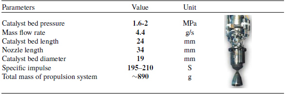
In this problem, a sample of a 10N monopropellant propulsion system is considered. Table 2, displays the main parameters related to this system [29].

Table 2.

Showing the shape and parameters of a 10N monopropellant propulsion system

Figure 4.

Display the objective functions, variables, and design responses for each of the subsystems.

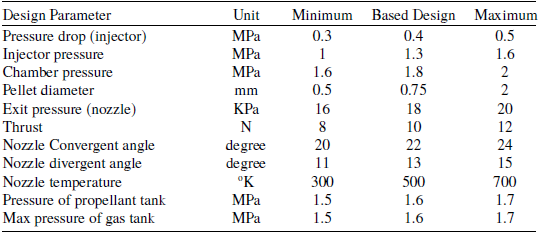
The design variables range for this system has been calculated using the mentioned relationships and is presented in Table 3.

3.0 DoE Based on LHS

The theory on where these design points should be placed in the design space to get the best possible information from a limited sample size is called DoE. The classical experimental designs are primarily used for screening purposes and as a base for building polynomial metamodels. When the dataset is used to fit a more complex metamodel, other experimental designs are preferred [Reference Ryberg, Domeij Bäckryd and Nilsson30].

The theories of DoE originate from planning physical experiments. The idea is to gain as much information as possible from a limited number of experiments. The methods focus on planning the experiments so that the random error from the physical experiments has minimum influence on the approval or disapproval of a hypothesis. Popular designs include factorial or fractional factorial designs, central composite designs, Box-Behnken designs, Koshal designs [Reference Ryberg, Domeij Bäckryd and Nilsson30] (Fig. 5).

Table 3.

The range of variations in the influential parameters of design for optimisation

Figure 5.

Display the experimental designs: a) full factorial design, b) central composite design, c) Box-Behnken design, and d) Koshal design [Reference Ryberg, Domeij Bäckryd and Nilsson30].

As mentioned earlier, the classical experimental designs focus on reducing the effect of noise in physical experiments. They also tend to spread the sample points around the border and only put a few points in the interior of the design space. Often many design variables are studied over a large design space and a proper experimental design for these cases should be space-filling, which aims to spread the design points within the complete design space [Reference Ryberg, Domeij Bäckryd and Nilsson30].

The first space-filling design, the LHS was proposed as a constrained random design [Reference Lin and Tang31]. For each of the k variables, the range of each variable is divided into n non-overlapping intervals of equal probability. One value from each interval is selected at random but for the probability density in the interval. The n values of the first variable are then paired randomly with the n values of the second variable. These n pairs are combined randomly with the n values of the third variable to form n triplets, and so on, until n k-tuplets are formed. This results in an n × k sampling plan matrix S, where the k columns describe the levels of each variable and the n rows describe the variable settings for each design, see Fig. 6 [Reference Ryberg, Domeij Bäckryd and Nilsson30].

Figure 6.

Normal and uniform distribution of two variables by LHS method [Reference Ryberg, Domeij Bäckryd and Nilsson30].

As mentioned above, the number of design points (NDP) for the LHS method is calculated using the formula ( $n \times k$ ), where (k) is the number of variables and (n) represents the number of levels. In this method, (n) does not follow a specific mathematical formula, but is determined by the user’s needs and computational budget. But there are a few key principles:

• • Minimum NDP should be at least as large as the number of variables, so that at least one unique level variable can be assigned to each variable.

• • For high accuracy in modeling, especially in meta-analytic methods (such as SVR or Kriging), the empirical ratio of 5k and 10k is often used. (5k is often used for smaller problems or when computational resources are limited, and 10k for more complex problems or higher accuracy requirements; this is a better choice [Reference McKay, Beckman and Conover32]).

In this paper, the NDP is calculated using the three-level full factorial method ( ${n^k}$ ), which is the maximum NDP in a deterministic method. The number obtained is considered as the NDP of the LHS method and the number of LHS levels is calculated based on it. Figure 7 shows the process of calculating the NDP for each subsystem with an example and also Fig. 8, shows the DoE process using the LHS method.

Figure 7.

The process of calculating the NDP.

Figure 8.

Present the DoE process [Reference Helton and Davis33].

4.0 Metamodel generation based on kriging

A surrogate model or metamodel is a simplified version of a real model. The metamodel can be a mathematical equation or algorithm that represents input-output relationships. Research for design exploration and simulation using metamodeling has been growing and remains an important research topic. With the increasing complexity of designs and associated costs for design and manufacturing technologies, the use of efficient and accurate metamodels is essential for reducing the design computational cost [Reference Okobiah, Mohanty and Kougianos34].

Kriging is a type of mathematical interpolation named after South African mining engineer Krige. This method was then formalised by French mathematician Matheron, who developed a new mathematical statistic called geostatistics or spatial statistics. The basis of this formalisation is the stationary Gaussian process (GP). This stationarity means that GP has a constant mean (expected value), a constant variance and covariances that depend only on the distances between ‘points’ in a k-dimensional space (e.g., length, width, height). It is obvious that in spatial statistics k ≤ 3. This GP represents a multivariate normal (or Gaussian) distribution [Reference Kleijnen35].

Recently in Refs (Reference Okobiah, Mohanty, Kougianos and Garitselov36, Reference Okobiah, Mohanty and Kougianos37), a study of different Kriging methods, simple, ordinary and universal is presented. Figure 9 shows a taxonomy of varying metamodeling techniques.

Figure 9.

Classification of metamodeling methods [Reference Okobiah, Mohanty and Kougianos34].

The proposed method for the simple Kriging (SK) metamodel generation in this study is summarised in Fig. 10. Figure 10 presents the detailed structure and procedure related to generation of the SK metamodel. In this step, the SK metamodel is generated using the design sample points produced by the LHS method. The generated metamodels must be validated before use for design exploration or optimisation. Validation tests ensure the accuracy of the metamodel and are usually done with additional random points through statistical analysis. In this study, the root mean square error (RMSE) and correlation coefficient (R2) measures are used to analyse the accuracy of the generated metamodels.

Figure 10.

Present of the Kriging meta-model generation process [Reference Santner, Williams and Notz38].

In Fig. 11, the proportionality of Kriging with linear regression is displayed in red. This operation solely represents the average of a normal distribution and the distribution can be utilised to present an estimation of uncertainty in Kriging predictions [Reference Brus, Heuvelink and de Gruijter39].

Figure 11.

Presenting the fit of Kriging with the linear regression model [Reference Brus, Heuvelink and de Gruijter39].

Since metamodels are unnecessary for low-fidelity analytical models, this paper demonstrates the optimisation framework by presenting and explaining the Kriging-based fitting of one subsystem. The other subsystems exhibit linear behaviour due to their analytical solutions.

4.1. Metamodeling of high-pressure gas tank mass

For the high-pressure gas storage tank, 81 points in the design space have been examined using the LHS method. Figure 12 illustrates the fitting of the model for the total mass of the high-pressure gas tank to the actual state using the Kriging method. Additionally, in this figure, the statistical data related to the total mass model of the high-pressure gas tank is provided to determine the accuracy and validity of the metamodel. According to the explanation, the R2, RMSE, predicted residual sum of squares (PRESS), etc. can serve as a basis for validating the generated metamodel. In this metamodel, based on Fig. 12, R2 is equal to one, RMSE is equal to zero, and PRESS has a value close to zero. Furthermore, in this fitting, the statistical data for the Kriging method is calculated using four functions, where the corresponding PRESS value for the Gaussian function is lower compared with the other functions, making it more suitable (Table 4).

Figure 12.

High-pressure gas tank mass metamodel.

5.0 Multi-objective optimisation using the SHERPA algorithm

Multi-objective optimisation is considered a field of multi-criteria decision-making. Multi-objective optimisation deals with mathematical optimisation problems in which more than one objective function needs to be simultaneously optimised. Mathematically, a multi-objective optimisation problem can be formulated as Equation (33) [Reference Jung, Choi and Kwon10].

(33) \begin{align}{\rm{mi}}{{\rm{n}}_{{\rm{x}} \in {\rm{X}}}}({{\rm{f}}_1}\left( {\rm{x}}\right)\!,{{\rm{f}}_2}\left( {\rm{x}} \right), \ldots ,{{\rm{f}}_{\rm{k}}}\left( {\rm{x}} \right)\end{align}

In which the integer $ k \gg 2$ , represents the number of goals and set X represents the set of feasible decision vectors, typically with X $ \in {\cal R}$ , but dependent on the n-dimensional domain of application. The set of feasibility is commonly defined by some constraint functions. Multi-objective optimisation poses a challenge as it is generally unfeasible to obtain a solution that minimises all objective functions simultaneously [Reference Hartikainen, Miettinen and Wiecek40]. Even for a basic multi-objective optimisation problem, the probability of discovering an optimal solution that optimises all defined objective functions concurrently is considerably low. This research undertakes a bi-objective optimisation, wherein the objective functions comprise maximising the specific impulse and minimising the mass of the propulsion system.

In numerous instances, the objective functions delineated in multi-objective optimisation problems exhibit inherent contradictions. Consequently, it is posited that the existence of Pareto optimal solutions is inevitable for a multi-objective optimisation problem (theoretically, a multi-objective optimisation problem may yield an infinite number of Pareto optimal solutions).

Table 4.

Performance evaluation criteria of the high-pressure gas tank mass metamodel

The SHERPA algorithm is a specialised search algorithm. The SHERPA algorithm is composed of an uncertain sorting process and guarantees that the optimal optimisation result is the best design that provides the predicted and expected answers [Reference Ngo, Bello-Ochende and Meyer41]. The SHERPA algorithm combines global and local search methods and automatically adjusts the tuning parameters. The features of the SHERPA algorithm are shown in Fig. 13 [42, Reference Hertel, Collado, Sadowski, Ott and Baldi43].

Figure 13.

The features of the SHERPA algorithm.

The SHERPA algorithm exists in two forms: weighted function and multi-objective. In this article, SHERPA tool, the multi-objective optimisation method, available in the commercial software HEEDS, has been used. The following are some features of this method.

It performs a multi-objective search using a modified version of the SHERPA algorithm. It independently manages multiple objectives to provide a set of optimal solutions and demonstrate the trade-offs between objectives. It employs multiple search strategies simultaneously to explore the Pareto front more effectively [42–Reference Chase, Rademacher, Goodman, Averill and Sidhu44].

Figure 14 presents a comparative graph illustrating the performance of different optimisation methods alongside the SHERPA algorithm [42].

Figure 14.

Comparison of various optimisation algorithms with the SHERPA algorithm [42, Reference Chase, Rademacher, Goodman, Averill and Sidhu44].

In this step, after verifying the accuracy of the constructed metamodels, the optimisation process is performed using the SHERPA algorithm with two objective functions: reducing the total system mass and increasing the specific impulse. Figure 15 illustrates a general framework for the optimisation process of this problem.

Figure 15.

Presenting the SHERPA optimisation framework [Reference Hertel, Collado, Sadowski, Ott and Baldi43].

As shown in Fig. 15, the optimisation outcomes derived from the Pareto diagram are presented in Fig. 16. The Pareto front represents the set of solutions where enhancing one objective would lead to a decline in another. This collection of solutions is non-dominant to one another and is more favourable than the remaining solutions within the search space. The diagram in Fig. 16 depicts the optimisation results according to the two axes of the objective functions (the highest value of specific impulse and the lowest mass of the entire system). The optimisation outcomes are illustrated as coloured circles of varying sizes on the graph. The colour of each circle indicates the optimal response to the conditions of the optimisation objective functions. In this way, the closer the circles are to the intersection of the two axes of the graph, the darker their blue colour becomes. This is because the responses of the objective functions can be satisfied by approaching the intersection of the two graphs. Also, the size of the circles indicates the degree of satisfaction of the objective functions. This means that the closer we get to the centre of the intersection of the two graphs, the smaller their sizes will be.

Typically, the nearest point to the intersection of two axes is the best answer with equal weight balance, unless the objective functions are different in terms of weight balance. In this study, assuming that the weight balance of the objective functions is equal, the closest point to the intersection of two axes is considered the best answer for this problem, which is also known as the knee point and is shown with a red circle on the graph. At the knee point, the objective function values are 224.443 s for specific impulse and 0.749 kg for the system’s total mass.

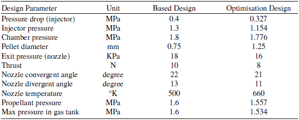
In the final step, the optimised model of the single-propellant liquid hydrazine thruster system was compared and evaluated with the baseline design model. Table 5 compares the design parameters at the knee point relative to the baseline design.

Table 5.

Comparison between design parameters at optimal point (knee point) and basic design

Figure 16.

Diagram of Pareto front and the knee point.

In Table 5, the optimal nozzle divergence angle is on the constraint boundary, and to reach the main optimum point, the relevant constraint range should be considered further. However, based on the results obtained in Table 6, the specific impulse has increased by 6% while the total system mass has decreased by 15.8%.

Table 6.

Comparison between optimisation objective functions with basic design

6.0 Conclusion

This article aims to introduce a novel synthesis optimisation framework based on a performance prediction model for a space propulsion system. Metamodels can potentially replace complex models while significantly reducing computational time and costs. Among these, Kriging – a nonlinear metamodeling technique – provides effective performance prediction and evaluation capabilities. The SHERPA algorithm, a robust, adaptive, and progressive multi-objective optimisation method, enables simultaneous hybrid search operations. The objective functions considered for optimisation in this study are the specific impulse and total mass of the propulsion system. In the output of multi-objective optimisation problems, multiple optimal points are introduced using the Pareto front, and the designer should select the desired design point considering all conditions. Typically, the knee point of the Pareto front is a balanced point between the objective functions. Finally, the obtained results are reported as follows:

• • The design variables of the maximum initial pressure of a high-pressure gas tank, the pressure of a liquid fuel tank, and thrust force have the greatest impact on the total mass of the propulsion system.

• • The design variables of pressure in the decomposition chamber and pressure of the liquid fuel reservoir are parameters that significantly affect the determination of the specific impulse. They have a direct relationship with the specific impulse.

• • At the knee point of the Pareto front, the values of the objective functions (specific impulse and total mass of the propulsion system) are 224.443 s and 749 g, respectively.

• • By using the SHERPA algorithm, the values of the objective functions have increased by 6% and the total mass of the system has decreased by 15.8% compared with the baseline design.