1 Introduction
Turbulence is a complex fluid flow phenomenon which emerges from the continuous reorganisation of the kinetic energy spatial distribution via local shear. The ubiquity of turbulence in nature entails that many manmade or biological entities are compelled to deal with it, influencing the dispersion in the oceans of contaminants (Toschi & Bodenschatz Reference Toschi and Bodenschatz2009; Cozar Reference Cozar2014) and controlling the formation of water droplets in clouds (Grabowski & Wang Reference Grabowski and Wang2013; Sardina et al. Reference Sardina, Picano, Brandt and Caballero2015), prey/predator encounter rates (Kiorboe Reference Kiorboe2008; Pecseli, Trulsen & Fiksen Reference Pecseli, Trulsen and Fiksen2012) or interactions of microplastics with local biota (Galloway, Cole & Lewis Reference Galloway, Cole and Lewis2017).
All these examples are characterised by the interaction between a turbulent flow and other entities which we will generically refer to as particles. Central to a proper understanding of particle–turbulence interactions is an accurate definition of the various time scales at play. Particle behaviour is necessarily associated with specific, case-dependent time scales. Turbulence, on the other hand, follows universal laws, at least when far from the boundary conditions and in homogeneous and isotropic conditions (Pope Reference Pope2000). A schematic view of turbulence is that it results from the multiple interactions between large- to intermediate-scale eddies which continuously transfer kinetic energy down to small scales, a process dubbed the inertial cascade of energy. At small scales, this energy is dissipated into heat down to the viscous scale (the so-called Kolmogorov length scale (Kolmogorov Reference Kolmogorov1958)
 $\unicode[STIX]{x1D702}_{K}=(\unicode[STIX]{x1D708}^{3}/\langle \unicode[STIX]{x1D700}\rangle )^{1/4}$
along with the corresponding time scale
 $\unicode[STIX]{x1D70F}_{K}=\sqrt{\unicode[STIX]{x1D708}/\langle \unicode[STIX]{x1D700}\rangle }$
, with
 $\unicode[STIX]{x1D708}$
the fluid kinematic viscosity and
 $\langle \unicode[STIX]{x1D700}\rangle$
the averaged dissipation) where no turbulent kinetic energy remains and the flow is therefore laminar. When travelling in the flow, a particle encounters various flow structures related to these eddies and viscous scales and undergoes rapidly changing dynamics. The resulting interaction of particles with turbulence can be direct (the particle size is larger than
 $\unicode[STIX]{x1D702}_{K}$
) or indirect (smaller than
 $\unicode[STIX]{x1D702}_{K}$
), and depends on whether the body is inertial and/or active, namely whether it acts or reacts against the flow (Toschi & Bodenschatz Reference Toschi and Bodenschatz2009). Here, we focus on non-inertial passive particles smaller than
 $\unicode[STIX]{x1D702}_{K}$
, and therefore neglect any potential feedback of the particle on the fluid.
Since particles are considered small, a first characteristic scale that could be considered for particle–turbulence interactions is the Kolmogorov scale; however, such a theoretical scale is derived from averaged quantities, hence losing the information on local spatial and temporal fluctuations of dissipation (Meneveau Reference Meneveau1996; Yu & Meneveau Reference Yu and Meneveau2010), with the result that
 $\unicode[STIX]{x1D702}_{K}$
does not accurately characterise the small scales of turbulence (Lazier & Mann Reference Lazier and Mann1989). These small-scale fluctuations are witness to the undergoing complex physics in turbulence. Namely, they cannot be simply modelled by Gaussian statistics, which, in light of the central limit theorem, implies that small-scale fluctuations are not independent from one another. Such a characteristic of turbulence is called intermittency (Chevillard et al.
Reference Chevillard, Castaing, Arneodo, Lévêque, Pinton and Roux2012).
The spatial and temporal characteristics of turbulence are usually studied respectively by considering the flow at fixed points (i.e. Eulerian frame of reference) and by following a given particle in the flow (Lagrangian frame of reference) (Pope Reference Pope2000). While Eulerian turbulence has been extensively studied for the past two centuries, deciphering the Lagrangian turbulence is on the contrary a younger topic only developed thanks to the combination of recent improvements in experimental techniques, used to track particles and measure the local properties of turbulence, continuous increases in computational power and development of new theoretical approaches (Toschi & Bodenschatz Reference Toschi and Bodenschatz2009). Statistical and scaling analyses using heavy numerical simulations along with theoretical modelling allowed for great improvements of our understanding of Lagrangian turbulence (Toschi & Bodenschatz Reference Toschi and Bodenschatz2009). We summarise below two significant characteristics of Lagrangian intermittency and related open questions to which we believe our study brings new information.
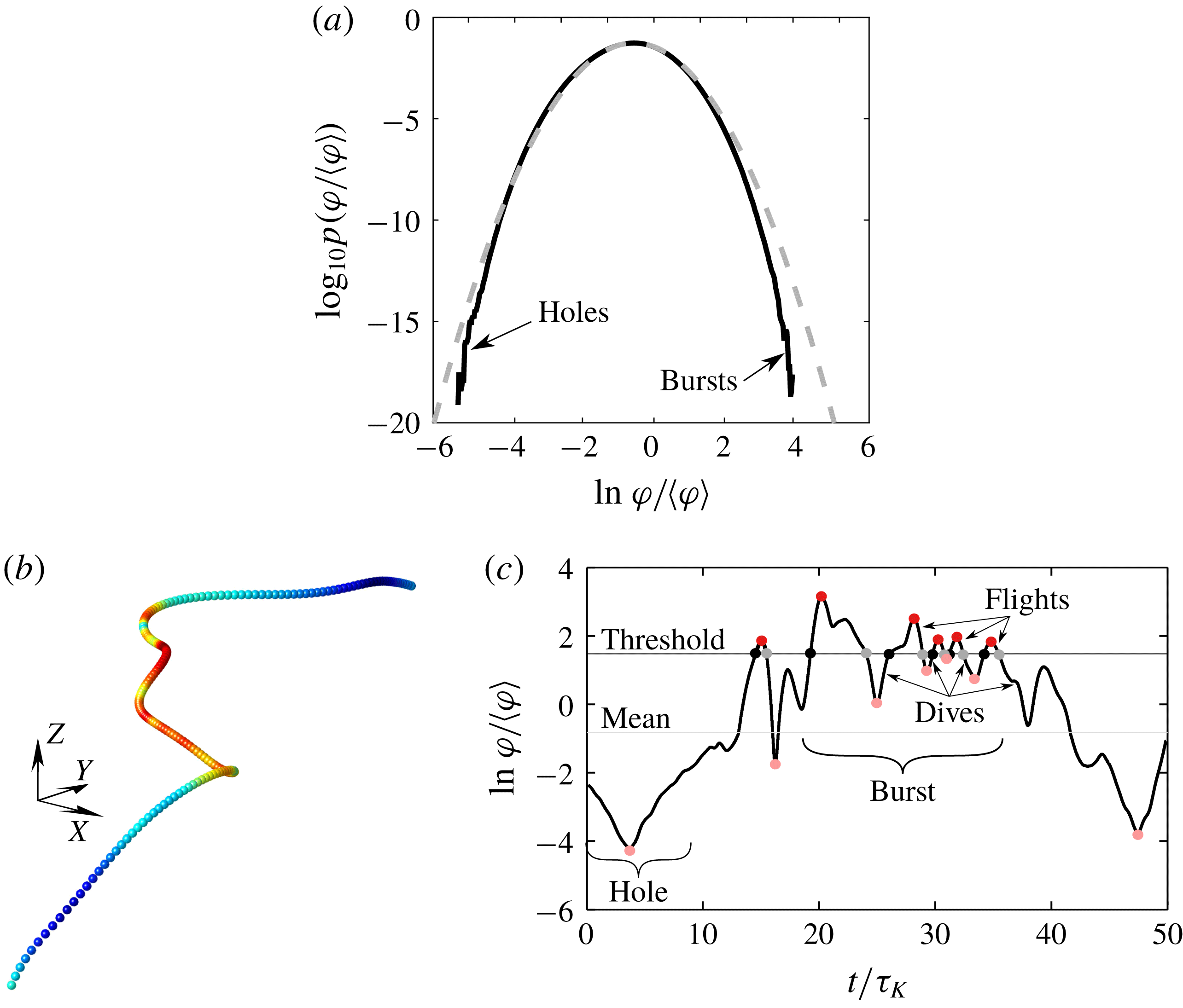
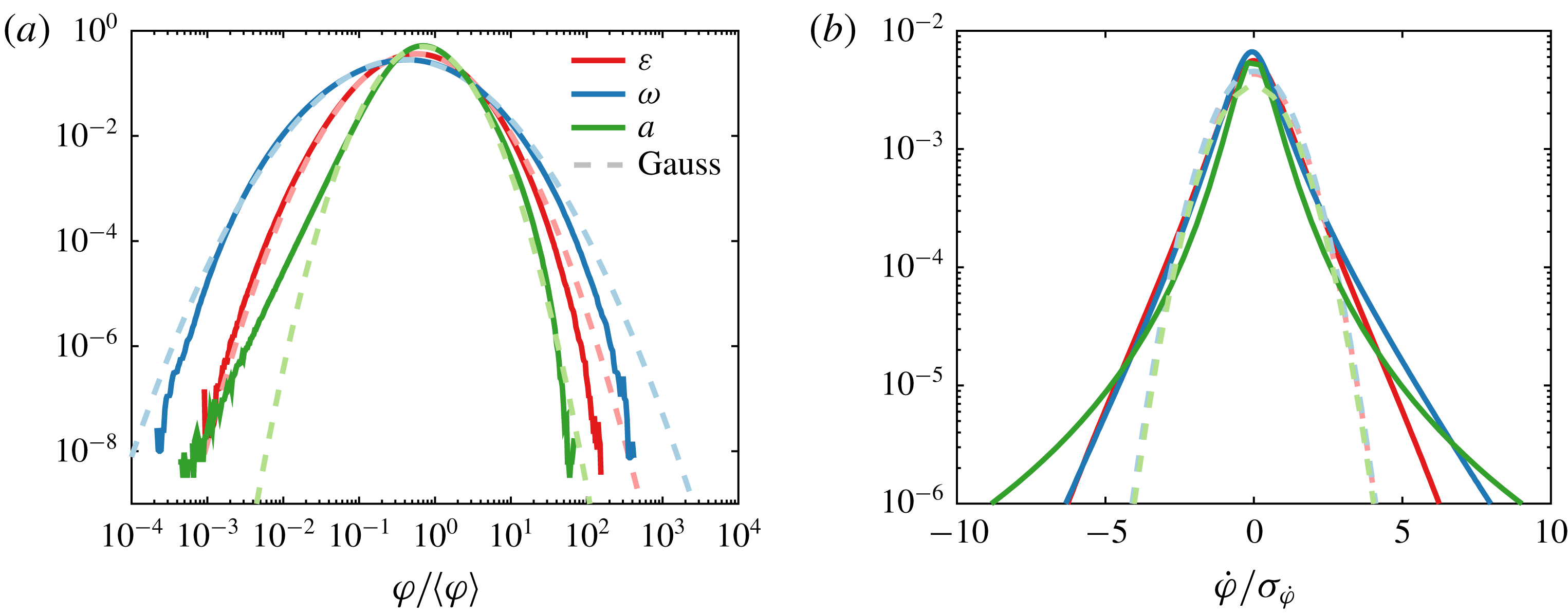
(a) Density profile of a Lagrangian turbulent quantity
 $\unicode[STIX]{x1D711}$
with log-normal approximation (dashed line). Bursts and holes create a departure from log-normal statistics. (b) Trajectory of a particle evolving in homogeneous isotropic turbulence (HIT). The colour map is
 $\ln \unicode[STIX]{x1D711}/\langle \unicode[STIX]{x1D711}\rangle$
. (c) Time series corresponding to the trajectory in (b). Given a threshold
 $\unicode[STIX]{x1D711}_{t}$
, flights and dives correspond to periods above (with maximum value in pure red) and below (with minimum value in light red)
 $\unicode[STIX]{x1D711}_{t}$
, respectively. Bursts and holes represent periods of large and small magnitude in
 $\unicode[STIX]{x1D711}$
. Finally, for both periods of bursts and holes, the computation of the various conditioned joint distributions of flights, transitions to dive, dives and transition to flight, shown in figure 8, is done by considering values associated with pure red, grey, light red and black dots, respectively.

First, the phenomenology of turbulence intermittency is usually linked to the random appearance (both in space and time) of bursts, namely, local and ephemeral events where properties of the flow such as the quantities of dissipation or acceleration attain very large magnitudes compared with their mean values (Pope Reference Pope2000). Eulerian studies on dissipation have suggested that, mirroring bursts, there also exist rare localised regions where quantities become very small, i.e. holes (Dubrulle Reference Dubrulle1994; She & Leveque Reference She and Leveque1994; She & Waymire Reference She and Waymire1995; Gledzer et al. Reference Gledzer, Villermaux, Kahalerras and Gagne1996). The simple consideration that turbulent quantities exhibit close to log-normal Lagrangian and Eulerian statistics (Yeung et al. Reference Yeung, Pope, Lamorgese and Donzis2006a ; Mouri Reference Mouri2015) (i.e. the order of magnitude of turbulent quantities have normal/Gaussian statistics) shows that there indeed exist a range of very low magnitudes which necessarily imply the presence of holes (figure 1 a). It is believed that holes are linked with intense vortical structures (She & Leveque Reference She and Leveque1994; Gledzer et al. Reference Gledzer, Villermaux, Kahalerras and Gagne1996), but such an assertion has never been investigated. Yet, the flow structures in turbulence are known to influence more the dynamical behaviour of Lagrangian particles than the detailed time history of the velocity field (Elhmaidi, Provenzale & Babiano Reference Elhmaidi, Provenzale and Babiano1993; Manikandan et al. Reference Manikandan, Haller, Peacok, Rupper-Felsot and Swinney2007). The characteristics of flow structures can be derived from the velocity invariants (Cantwell Reference Cantwell1993; Soria et al. Reference Soria, Sondergaard, Cantwell, Chong and Perry1994; Martin et al. Reference Martin, Ooi, Chong and Soria1998; Ooi et al. Reference Ooi, Martin, Soria and Chong1999).
Second, intermittency results from the non-trivial combination of the dynamics of inertial (large to intermediate) and dissipative (small) scales. In the inertial range, the dynamics behind eddy interactions is self-similar (Kolmogorov Reference Kolmogorov1958), namely, it can be captured by considering that eddies behave equivalently regardless the eddy scale and that therefore only the magnitude of turbulent fluctuations varies. This feature can be modelled by considering eddy interactions as a multiplicative process across scale, hence explaining why the statistics of the turbulent quantities are close to log-normal (Yeung et al. Reference Yeung, Pope, Lamorgese and Donzis2006a ; Mouri Reference Mouri2015). However, the departure from log-normal (figure 1 a) at small and large magnitudes shows that holes and bursts have a more complex dynamics and that the multiplicative vision of turbulence only holds somewhat true for moderate magnitudes of turbulent quantities. Besides, even at moderate magnitude, the multiplicative approach fails to give good predictions for high moments of the fluctuations (Benzi et al. Reference Benzi, Ciliberto, Tripiccione, Baudet, Massaioli and Succi1993, Reference Benzi, Biferale, Fisher, Lamb and Toschi2010). By being responsible for the departure from log-normal statistics, holes and bursts are therefore at the core of turbulence intermittency and the non-self-similar patchy and inconstant nature of the flow. The multifractal formalism (associated with generalised multiplicative processes) accurately captures this non-self-similar characteristic of turbulence in the inertial cascade (Frisch Reference Frisch, Ghil, Benzi and Parisi1983; Benzi et al. Reference Benzi, Paladin, Parisi and Vulpiani1984; Meneveau & Sreenivasan Reference Meneveau and Sreenivasan1987), but other methods can also be good predictors (Huang et al. Reference Huang, Biferale, Calzavarini, Sun and Toschi2013).
Along with the impact of the inertial range on bursts and holes is that of the dissipative range, where large fluctuations of quantities due to eddy interactions are smoothed out by viscosity. Classical multifractal formalism considering only one scale (
 $\unicode[STIX]{x1D702}_{K}$
) fails to capture the local dynamics of dissipation in the dissipative range, and only by considering a local and variable scale can one capture the Lagrangian statistics at small scale (Sirovich, Smith & Yakhot Reference Sirovich, Smith and Yakhot1994; Meneveau Reference Meneveau1996; Arneodo et al.
Reference Arneodo2008; Benzi et al.
Reference Benzi, Biferale, Fisher, Lamb and Toschi2010; Yu & Meneveau Reference Yu and Meneveau2010). Such statistics, the so-called anomalous statistics, emerge in Lagrangian turbulence on time scales of
 $[1{-}10]\unicode[STIX]{x1D70F}_{K}$
(Biferale et al.
Reference Biferale, Boffetta, Celani, Lanotte and Toschi2005; Arneodo et al.
Reference Arneodo2008). Yet, how exactly inertial and dissipative scales generate such dynamics and how it relates to the presence of both bursts and holes is still not clearly understood. Such an unknown is however believed to be one of the greatest barriers to overcome in both stochastic modelling and theory of Lagrangian turbulence (Sawford Reference Sawford2001; Yakhot & Sreenivasan Reference Yakhot and Sreenivasan2005; Zybin et al.
Reference Zybin, Sirota, Ilyin and Gurevich2008; Benzi et al.
Reference Benzi, Biferale, Fisher, Lamb and Toschi2010).
Central to these open problems is the small-scale temporal structure of the Lagrangian turbulence properties i.e. Lagrangian intermittency. Deciphering its characteristics has been a point of attention for a few decades (Yeung Reference Yeung2002; Toschi & Bodenschatz Reference Toschi and Bodenschatz2009) and we shall now briefly explain the various findings (however in a non-exhaustive manner) and the questions that remain on hold to which we believe this study brings some elements of an answer. Lagrangian intermittency was mainly studied by focusing on the moments of the fluctuations of the velocity
 $\langle (v(t+\unicode[STIX]{x1D70F})-v(t))^{p}\rangle$
(i.e. the Lagrangian structure functions of order
 $p$
) (e.g. Benzi et al.
Reference Benzi, Paladin, Parisi and Vulpiani1984; Meneveau & Sreenivasan Reference Meneveau and Sreenivasan1987; Yeung Reference Yeung2001; Boffetta, De Lillo & Musacchio Reference Boffetta, De Lillo and Musacchio2002; Ouellette et al.
Reference Ouellette, Xu, Bourgoin and Bodenschatz2006; Arneodo et al.
Reference Arneodo2008; Biferale et al.
Reference Biferale, Bodenschatz, Cencini, Lanotte, Ouellette, Toschi and Xu2008; Chevillard et al.
Reference Chevillard, Castaing, Arneodo, Lévêque, Pinton and Roux2012) which helped to detect the aforementioned so-called anomalous statistics. Because of the averaging process, the structure functions are a powerful tool to investigate the global change of turbulence but cannot detect recurrences. Moreover, study of (i) the Lagrangian Taylor time scale, i.e. the time scale associated with the variation rate of the velocity for short periods of time (e.g. Tennekes Reference Tennekes1975; Yeung & Pope Reference Yeung and Pope1989; Ishihara & Kaneda Reference Ishihara and Kaneda1993; Kaneda Reference Kaneda1993; Yeung Reference Yeung2001)
 $$\begin{eqnarray}\unicode[STIX]{x1D70F}_{L,v}=\frac{\unicode[STIX]{x1D70E}_{v}}{\unicode[STIX]{x1D70E}_{\text{d}v/\text{d}t}},\end{eqnarray}$$
and (ii) the decorrelation time scale of different tubulence quantities (velocity, dissipation, etc.), i.e. the time window after which information of the previous fluctuations of
 $\unicode[STIX]{x1D711}$
is lost (e.g. Pope Reference Pope1990; Squires & Eaton Reference Squires and Eaton1991; Mordant et al.
Reference Mordant, Delour, Leveque, Arneodo and Pinton2002)
 ${\mathcal{T}}_{\unicode[STIX]{x1D711}}=\int _{0}^{\infty }\unicode[STIX]{x1D70C}_{\unicode[STIX]{x1D711}}(\unicode[STIX]{x1D70F})\,\text{d}\unicode[STIX]{x1D70F}$
with
 $\unicode[STIX]{x1D70C}_{\unicode[STIX]{x1D711}}$
the autocorrelation coefficient of
 $\unicode[STIX]{x1D711}$
, also highlighted a complex physics lying behind Lagrangian intermittency with a strong dependency on the level of turbulence. However, both the dimensional scaling and statistical averaging used to infer
 $\unicode[STIX]{x1D70F}_{L,\unicode[STIX]{x1D711}}$
and
 ${\mathcal{T}}_{\unicode[STIX]{x1D711}}$
destroy part of the physical information potentially relevant for understanding Lagrangian intermittency and, as a consequence, these two time scales may mix scaling relations of different regimes (Wang Reference Wang2014). This, in turn, makes it difficult to understand what these time scales exactly represent to the travelling particle subjected to Lagrangian fluctuations and how they relate to the local and ephemeral bursts and holes.
With the aim of disentangling the various multiscale contributions to turbulence and potentially characterising better the dynamics behind Lagrangian fluctuations and its relation to flow structures, other methods have been used, consisting essentially in decomposing the signals following a given procedure. A first approach was to study the power spectra of Lagrangian signals using the widespread discrete Fourier transform (Tennekes & Lumley Reference Tennekes and Lumley1972; Sreenivasan & Stolovitzky Reference Sreenivasan and Stolovitzky1995; Yeung Reference Yeung2001), revealing a range of frequencies in which exists a constant scaling (and where therefore the dynamics is self-similar). This former range is however much narrower than the inertial range, reflecting spurious contributions from regimes of other scales (either large or small) that the Fourier transform could not disentangle. Such an issue is also present in the statistics of structure functions (Sawford & Yeung Reference Sawford and Yeung2011), thus showing the impact of the methods of analysis for the study of multiscale physical phenomena. A new method based on empirical mode decomposition, called the Hilbert–Huang Transform (HHT) (Huang et al. Reference Huang, Shen, Long, Wu, Shih, Zheng, Yen, Chao Tung and Liu1998), was applied to Lagrangian fluctuations (Huang et al. Reference Huang, Biferale, Calzavarini, Sun and Toschi2013) and revealed a clear inertial-range unique scaling, but explaining the phenomenology of the flow from HHT is still in the early stages.
In order to avoid potential transformation-based discrepancies and to use more quantitative methods, various more direct methods were developed to cut the Lagrangian signals into segments and study the distribution of the corresponding time scales. Since Lagrangian intermittency is tightly linked to the flow structures, some methods cut the Lagrangian signals following physical considerations based on the Eulerian flow structures (Martin et al.
Reference Martin, Ooi, Chong and Soria1998; Ooi et al.
Reference Ooi, Martin, Soria and Chong1999; Liberzon et al.
Reference Liberzon, Lüthi, Holzner, Ott, Berg and Mann2012; Wang Reference Wang2014; Bhatnagar et al.
Reference Bhatnagar, Gupta, Mitra, Pandit and Perlekar2016). For instance, Wang (Reference Wang2014) cuts the signals into segments using extrema of the acceleration, considered as a proxy for passage from the vortex- to the stretching-dominated regions. By deriving the time distribution corresponding to the segments and conditioning the velocity and dissipation statistics to this time of transition, this method revealed a constant scaling across the inertial range, therefore showing that conditioning the statistics on the flow structures could help in removing the multiscale contamination. The mean time of transition between vortical and straining structures scales was the viscous scale
 $\unicode[STIX]{x1D70F}_{K}$
, showing that studying the extrema of acceleration sheds light primarily on small-scale dynamics. On the contrary, other studies focused on large-scale dynamics of Lagrangian fluctuations by using velocity invariants to study the time distribution of the residence (or persistence) times in the various vortical and straining flow structures (Martin et al.
Reference Martin, Ooi, Chong and Soria1998; Ooi et al.
Reference Ooi, Martin, Soria and Chong1999; Bhatnagar et al.
Reference Bhatnagar, Gupta, Mitra, Pandit and Perlekar2016) with the outcome that particles mainly remain in specific flow structures on the time scale of large eddies with power-law or exponential time distributions.
Another method of interest used to study intermittency is to derive the distribution of the zero-crossing time scales, namely, the distribution of residence times above and below zero velocity. Such a method has been used to characterise Eulerian bursts and fine-scale intermittency in turbulent boundary layers (Narahari Rao, Narasimha & Badrinarayanan Reference Narahari Rao, Narasimha and Badrinarayanan1971; Badrinarayanan, Rajagopalan & Narasimha Reference Badrinarayanan, Rajagopalan and Narasimha1977; Sreenivasan, Prabhu & Narasimha Reference Sreenivasan, Prabhu and Narasimha1983; Sreenivasan Reference Sreenivasan1985; Kailasnath & Sreenivasan Reference Kailasnath and Sreenivasan1993). These studies also relied on the accompanying theory of zero crossings (Rice Reference Rice1945; Liepmann Reference Liepmann1949; Ylvisaker Reference Ylvisaker1965) which states, among other things, that if
 $g$
is a Gaussian process with mean
 $g_{m}$
(taken originally to be 0), then the associated mean frequency of
 $g_{m}$
-crossings,
 $N_{g_{m}}$
(with
 $1/N_{g_{m}}$
the mean time spent between two successive crossings), is proportional to the Taylor-type time scale, following
 $$\begin{eqnarray}\unicode[STIX]{x1D70F}_{E,g}=\frac{\unicode[STIX]{x1D70E}_{g}}{\unicode[STIX]{x1D70E}_{\text{d}g/\text{d}t}}=\frac{1}{\unicode[STIX]{x03C0}N_{g_{m}}}.\end{eqnarray}$$
Hence, considering
 $\unicode[STIX]{x1D70F}_{L,g}$
as the Lagrangian version of
 $\unicode[STIX]{x1D70F}_{E,g}$
, one has that, for a Gaussian process,
 $\unicode[STIX]{x1D70F}_{E/L,g}$
scales with the mean residence time spent above or below its mean value. The rescaled Eulerian Taylor time scale
 $\unicode[STIX]{x03C0}\unicode[STIX]{x1D70F}_{E,g}$
has been shown to be a good approximation of the mean residence time also for various non-Gaussian distributions (Sreenivasan et al.
Reference Sreenivasan, Prabhu and Narasimha1983). In these studies, most of the attention has been given to finding the appropriate parameters to characterise mathematically turbulent intermittency. Here, we mainly study the phenomenology of Lagrangian intermittency and we shall only mention the outcomes that bear interest for our purposes. First, it has been found that the relationship between the Taylor scale and
 $0$
-crossing frequency holds true enough even for a non-Gaussian process, such as the turbulent velocity along a boundary layer, possibly due to the fact that the highly probable events of
 $u$
behind the zero crossings follow a Gaussian distribution (by considerations of the central limit theorem) even if the overall probability density function (p.d.f.) is non-Gaussian (Kailasnath & Sreenivasan Reference Kailasnath and Sreenivasan1993). Second, the distribution of zero-crossing intervals can be separated into two different exponentially decreasing parts at large and small time intervals (Sreenivasan et al.
Reference Sreenivasan, Prabhu and Narasimha1983), supposedly reflecting the long intervals of passage inside large-scale structures, each passing being independent of the others, while the short intervals are due to the small-scale dissipative structures riding on the large structures (Sreenivasan et al.
Reference Sreenivasan, Prabhu and Narasimha1983; Kailasnath & Sreenivasan Reference Kailasnath and Sreenivasan1993). Such an interpretation suggests that a selective conditional sampling technique based on zero crossings can be useful in separating the properties of large and small structures in turbulent shear flows (Sreenivasan et al.
Reference Sreenivasan, Prabhu and Narasimha1983; Kailasnath & Sreenivasan Reference Kailasnath and Sreenivasan1993; Cava & Katul Reference Cava and Katul2009; Cava et al.
Reference Cava, Katul, Molini and Elefante2012; Chamecki Reference Chamecki2013). Finally, Eulerian bursts in signals were analysed (Narahari Rao et al.
Reference Narahari Rao, Narasimha and Badrinarayanan1971; Badrinarayanan et al.
Reference Badrinarayanan, Rajagopalan and Narasimha1977; Sreenivasan et al.
Reference Sreenivasan, Prabhu and Narasimha1983; Sreenivasan Reference Sreenivasan1985). Bursts were considered as high-frequency pulses and their detection was made by determining the threshold above zero velocity at which the crossing frequency of the envelope of the signal (i.e. the signal obtained by considering only the maxima of fluctuations) was the highest. Such a technique was employed by considering the envelope of various bandpass filters of the Eulerian turbulent signals. Although this technique was useful in dissecting regions of high activity in the signal, it is computationally heavy to apply when considering millions of trajectories, and its complexity renders difficult the physical interpretation of results (Sreenivasan Reference Sreenivasan1985). Hence, the results were mainly interesting in regard to setting and studying some of the intermittency parameters as functions of the crossing level (and indirectly the bandpass filtering); however, conclusions about the characterisation of the dynamics underlying the signal fluctuations remained preliminary and bound to the crucial question raised by Sreenivasan (Reference Sreenivasan1985), that is, ‘What is the correct threshold setting that one should choose to define the parameters of intermittency?’, the answer to which depends on the dynamical characteristics of the signal. Finally, the technique suffers from its dependency on Fourier transforms which, as previously mentioned, do not separate properly the small to large scales.
Despite the clear interest of the theory of zero crossings and its results, to our knowledge, only a few studies, focusing on aggregate break-ups in turbulence, have used the method of crossing frequencies in a Lagrangian framework to study ‘diving’ residence times below various magnitudes of dissipation (Babler, Biferale & Lanotte Reference Babler, Biferale and Lanotte2012; Babler et al.
Reference Babler, Biferale, Brandt, Feudel, Guseva, Lanotte, Marchioli, Picano, Sardina and Soldati2014). Yet, temporal statistics emerging from the zero-crossing approach represent another interesting manner to detect and study Lagrangian intermittency in turbulence and to assess the accuracy of Lagrangian stochastic models. Here, we study the Lagrangian fluctuations of homogeneous isotropic turbulence (HIT) by analysing the flying and diving Lagrangian probability density functions (flying LPDF and diving LPDF) and corresponding flying and diving joint distributions of velocity invariants of various turbulent quantities. Given the time evolution of any quantity
 $\unicode[STIX]{x1D711}$
along a Lagrangian trajectory, the flying and diving LPDFs
 ${\mathcal{P}}_{\unicode[STIX]{x1D711}_{t}}^{F}(\unicode[STIX]{x1D70F})$
and
 ${\mathcal{P}}_{\unicode[STIX]{x1D711}_{t}}^{D}(\unicode[STIX]{x1D70F})$
represent the density of probability that
 $\unicode[STIX]{x1D711}$
spends some time
 $\unicode[STIX]{x1D70F}$
above (a flying event) and below (a diving event) a chosen threshold
 $\unicode[STIX]{x1D711}_{t}$
(figure 1
b,c). In order not to make notations heavier, i.e.
 ${\mathcal{P}}_{\unicode[STIX]{x1D711}_{t},\unicode[STIX]{x1D711}}^{F}(\unicode[STIX]{x1D70F})$
,
 $\unicode[STIX]{x1D711}_{t}$
indicates both the threshold and the quantity
 $\unicode[STIX]{x1D711}$
considered. For each quantity, flying and diving LPDFs are inferred for various crossing thresholds scanning the entire range of available magnitudes, hence avoiding the problem of defining one specific threshold to detect bursts and holes. Our analysis then focuses on properties of the temporal statistics of Lagrangian bursts and holes which consistently appear across the range of large and small thresholds, respectively. Study of the corresponding flying and diving joint distributions of velocity invariants allows us to describe the local Eulerian flow characteristics surrounding the particle during flights and dives across the chosen thresholds used to detect the Lagrangian bursts or holes. We end our study by developing a theoretical approximation of the mean flying and diving times in HIT and using the newly computed Lagrangian statistics to assess the accuracy of existing Lagrangian stochastic models.
Finally, turbulence is a multiscale process both in space and time and, as such, it is fair to suppose that the sensitivity of such a process is also scale dependent. For instance, diving times of
 $30\unicode[STIX]{x1D70F}_{K}$
and
 $40\unicode[STIX]{x1D70F}_{K}$
hold the same large-scale physical information while diving times of
 $\unicode[STIX]{x1D70F}_{K}$
and
 $10\unicode[STIX]{x1D70F}_{K}$
(viscous and inertial scales) do not. This suggests that
 ${\mathcal{P}}_{\unicode[STIX]{x1D711}_{t}}^{D}(\unicode[STIX]{x1D70F})$
can be a relevant distribution when focusing on a specific physics, either on a small or large scale (as pointed out by Sreenivasan et al. (Reference Sreenivasan, Prabhu and Narasimha1983)), but not for the inertial range where the multiscale aspect of turbulence is strongest. In statistical terms, this means that it is more relevant to compare probabilities with relative uncertainties, for instance, to compare the probability of a diving time of
 $35\unicode[STIX]{x1D70F}_{K}\pm 5\,\%$
and that of
 $5\unicode[STIX]{x1D70F}_{K}\pm 5\,\%$
rather than those of
 $35\unicode[STIX]{x1D70F}_{K}\pm 5\unicode[STIX]{x1D70F}_{K}$
and
 $5\unicode[STIX]{x1D70F}_{K}\pm 5\unicode[STIX]{x1D70F}_{K}$
. Such requirements are easily fulfilled with continuous density functions by studying
 ${\mathcal{P}}_{\unicode[STIX]{x1D711}_{t}}^{D}(\ln \unicode[STIX]{x1D70F})$
instead of
 ${\mathcal{P}}_{\unicode[STIX]{x1D711}_{t}}^{D}(\unicode[STIX]{x1D70F})$
. Such an assumption has already been made for distance in the Eulerian framework by Sreenivasan & Bershadskii (Reference Sreenivasan and Bershadskii2006) for whom this approach seemed reasonable because the scale-to-scale energy transfer in turbulence is presumed to occur in logarithmically equal intervals. We believe the same occurs with time.
2 Setting of the study
We study the temporal statistics of three turbulence quantities commonly used to study intermittency (Yeung & Pope Reference Yeung and Pope1989; Yeung, Pope & Sawford Reference Yeung, Pope and Sawford2006b
; Liberzon et al.
Reference Liberzon, Lüthi, Holzner, Ott, Berg and Mann2012), namely, acceleration,
 $a_{i}=\text{d}u_{i}/\text{d}t$
, rate-of-strain
 $\unicode[STIX]{x1D61A}_{ij}=(\unicode[STIX]{x1D608}_{ij}+\unicode[STIX]{x1D608}_{ji})/2$
and rate-of-rotation,
 $\unicode[STIX]{x1D61E}_{ij}=(\unicode[STIX]{x1D608}_{ij}-\unicode[STIX]{x1D608}_{ji})/2$
, where
 $t$
is time and
 $\unicode[STIX]{x1D608}_{ij}=\unicode[STIX]{x2202}_{i}u_{j}$
is the velocity gradient tensor. Their respective magnitudes can be quantified using the norm of the acceleration
 $|\boldsymbol{a}|$
, the dissipation rate of turbulent kinetic energy
 $\unicode[STIX]{x1D700}=2\unicode[STIX]{x1D708}\unicode[STIX]{x1D61A}_{ij}\unicode[STIX]{x1D61A}_{ij}$
and the enstrophy
 $\unicode[STIX]{x1D714}=2\unicode[STIX]{x1D708}\unicode[STIX]{x1D61E}_{ij}\unicode[STIX]{x1D61E}_{ij}$
, where
 $\unicode[STIX]{x1D708}$
is the kinematic viscosity. We therefore study the flying LPDF and diving LPDF,
 ${\mathcal{P}}_{\unicode[STIX]{x1D711}_{t}}^{F}(\ln \unicode[STIX]{x1D70F})$
and
 ${\mathcal{P}}_{\unicode[STIX]{x1D711}_{t}}^{D}(\ln \unicode[STIX]{x1D70F})$
, for
 $\unicode[STIX]{x1D711}=\unicode[STIX]{x1D700}$
,
 $|\boldsymbol{a}|$
(henceforth called
 $a$
) and
 $\unicode[STIX]{x1D714}$
at various thresholds
 $\unicode[STIX]{x1D711}_{t}$
. It is important to note that the flying and diving LPDFs are transformation invariants e.g.
 ${\mathcal{P}}_{\unicode[STIX]{x1D711}_{t}}^{F}(\ln \unicode[STIX]{x1D70F})={\mathcal{P}}_{\ln \unicode[STIX]{x1D711}_{t}}^{F}(\ln \unicode[STIX]{x1D70F})$
. This interesting property will be used below for theoretical derivation of the mean times. Finally, the flying and diving joint probability density functions of the velocity invariants are derived for all three quantities using various thresholds to isolate bursts and holes.
2.1 Numerical simulation set-up
We use a combined Eulerian–Lagrangian framework to compute a homogeneous isotropic turbulent (HIT) flow. The computational domain is a cube with periodic boundary conditions in all three spatial directions. The same numerical code as in Sardina et al. (Reference Sardina, Picano, Brandt and Caballero2015) is used, with the difference that a component-specific volume forcing term
 $f_{i}$
is used, following in Fourier space
 $$\begin{eqnarray}\hat{f}_{i}(k_{i},t)=\left\{\begin{array}{@{}ll@{}}\langle \unicode[STIX]{x1D700}\rangle \displaystyle \frac{\hat{u} _{i}(k_{i},t)}{\displaystyle \mathop{\sum }_{|k_{i}|}3|\hat{u} _{i}(k_{i},t)|^{2}} & \text{for }k_{min}\leqslant |k_{i}|\leqslant k_{max},\\ 0 & \text{otherwise},\end{array}\right.\end{eqnarray}$$
where the symbol
 $\hat{\ast }$
indicates the Fourier transformation of the generic real function *,
 $\langle \unicode[STIX]{x1D700}\rangle$
is the prescribed turbulent dissipation rate,
 $k_{min}$
and
 $k_{max}$
are the wavelengths limits influenced by the forcing. Such a forcing method, already successfully used for the computation of HIT (Carati, Ghosal & Moin Reference Carati, Ghosal and Moin1995; Watteaux, Stocker & Taylor Reference Watteaux, Stocker and Taylor2015), has the advantage of adjusting independently the three velocity components in order to achieve an accurate isotropic flow. Here, we force all Fourier components between
 $k_{min}=2.44$
and
 $k_{max}=3.09$
. Our spatial resolution consists of
 $1024^{3}$
grid points, chosen to give a Taylor Reynolds number of
 $Re_{\unicode[STIX]{x1D706}}$
of
 $240$
according to the constraints previously prescribed for direct numerical simulation (DNS) of HIT (Donzis, Yeung & Sreenivasan Reference Donzis, Yeung and Sreenivasan2008). While not the finest resolution used for the study of Lagrangian statistics in HIT (Yeung et al.
Reference Yeung, Pope and Sawford2006b
), it still creates a flow that can largely be considered turbulent. The time step is
 $\unicode[STIX]{x1D70F}_{K}/40$
and therefore ensures a well-resolved temporal sampling of the Lagrangian statistics. The total simulation time corresponds to
 $T=245\unicode[STIX]{x1D70F}_{K}$
and to
 $2.6{\mathcal{T}}_{u}$
. Approximately
 $10^{6}$
particles were tracked, saving all the relevant observables along their trajectories at every time step. This large number of particles ensures that our one-particle one-time Lagrangian statistics are equivalent to single-point Eulerian statistics. The same simulation at
 $Re_{\unicode[STIX]{x1D706}}=90$
was conducted in order to assess the dependency of our results on the Reynolds number.
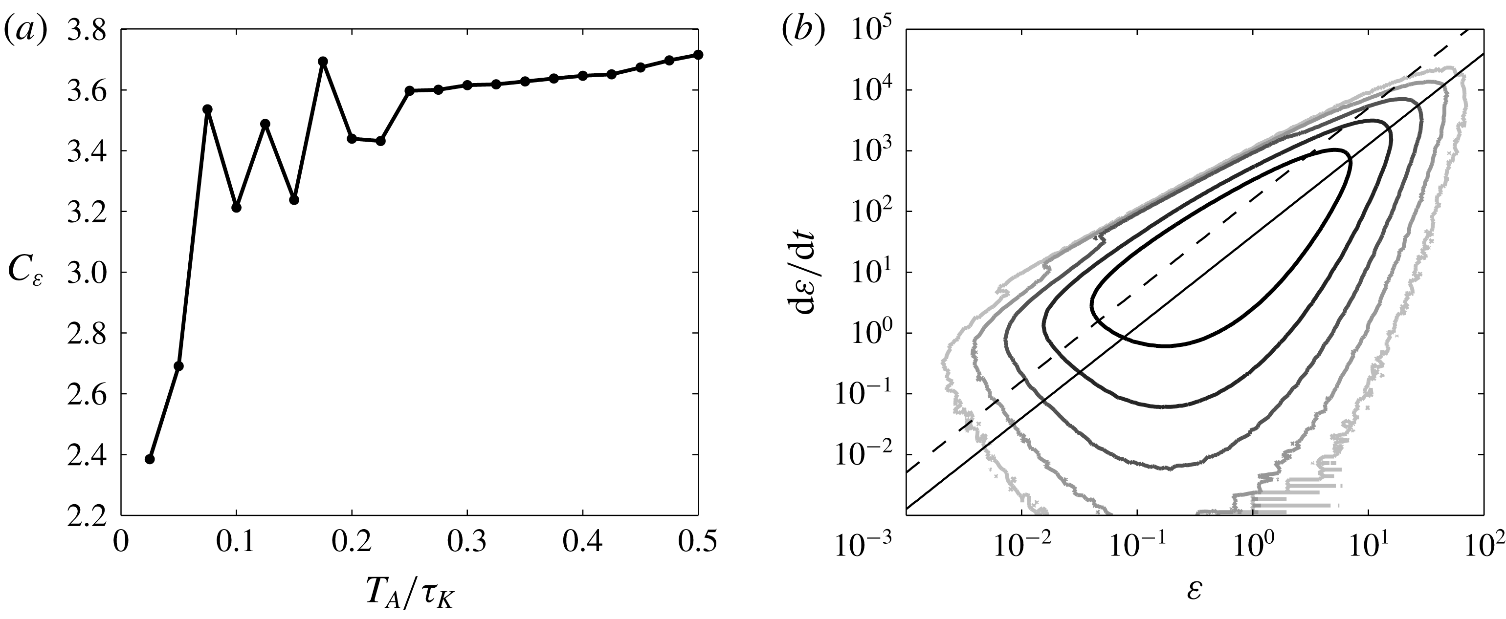
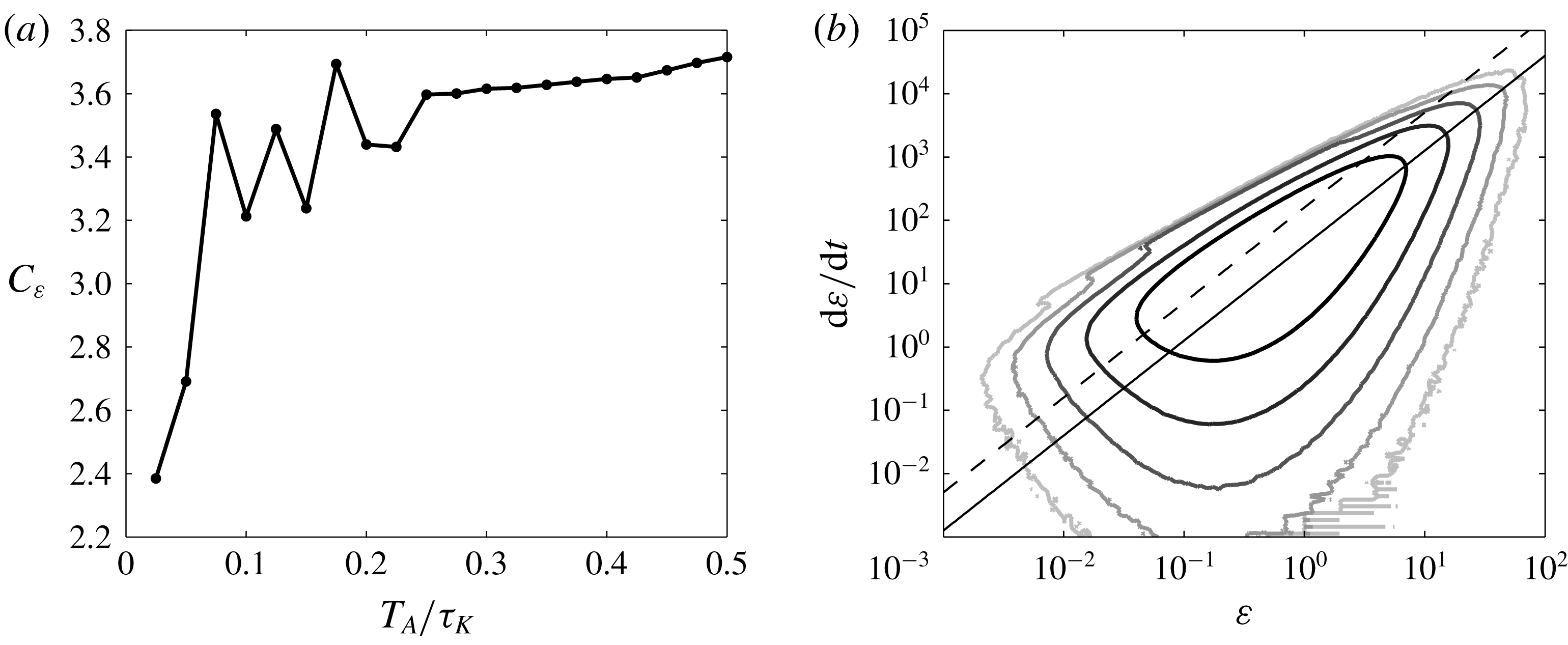
The principal direction of
 $p_{2}(\unicode[STIX]{x1D700},\dot{\unicode[STIX]{x1D700}})$
can be approximated by the relation
 $\dot{\unicode[STIX]{x1D700}}=\unicode[STIX]{x1D700}/C_{\unicode[STIX]{x1D700}}\unicode[STIX]{x1D70F}_{K}(\unicode[STIX]{x1D700})$
where
 $\unicode[STIX]{x1D70F}_{K}(\unicode[STIX]{x1D700})=(\unicode[STIX]{x1D708}/\unicode[STIX]{x1D700}^{3})^{1/4}$
is the local viscous scale and
 $C_{\unicode[STIX]{x1D700}}$
the coefficient to be determined. The Lagrangian time series are noisy due to discrepancies in the interpolation method and a weighted moving filter with characteristic time
 $T_{A}$
is applied to the signals. The coefficient
 $C_{\unicode[STIX]{x1D700}}$
is derived by taking the principal orientation of the filtered
 $p_{2}$
. (a)
 $C_{\unicode[STIX]{x1D700}}$
as a function of
 $T_{A}$
which stabilises at
 $3.6$
for
 $T_{A}=\unicode[STIX]{x1D70F}_{K}/3$
, and (b)
 $p_{2}(\unicode[STIX]{x1D700},\dot{\unicode[STIX]{x1D700}})$
using
 $T_{A}=\unicode[STIX]{x1D70F}_{K}/3$
with, in solid line, the corresponding scaling
 $\unicode[STIX]{x1D700}/C_{\unicode[STIX]{x1D700}}\unicode[STIX]{x1D70F}_{K}(\unicode[STIX]{x1D700})$
using
 $C_{\unicode[STIX]{x1D700}}=3.6$
and in the dashed line that of
 $p_{2}$
when using raw data. When not filtering dissipation, fluctuations in time are larger and therefore
 $C_{\unicode[STIX]{x1D700}}$
decreases.
2.2 Filtering of spurious Lagrangian statistics
Physical turbulence quantities at particles position are inferred from the Eulerian grid using a tri-linear interpolation. While such a scheme represents a quick and accurate method for interpolation of the velocity, it is known to create unphysical noise in the Lagrangian time series of higher-order quantities (van Hinsberg et al. Reference van Hinsberg, ten Thije Boonkkamp, Toschi and Clercx2013) which in turn parasites the flying and diving LPDFs. To circumvent this issue, we convolute all Lagrangian time series with a weighted moving average filter of the form
 $$\begin{eqnarray}A(t)=\left\{\begin{array}{@{}ll@{}}(t+T_{A})/T_{A}^{2} & \text{if }-T_{A}<t<0,\\ -(t-T_{A})/T_{A}^{2} & \text{if }0<t<T_{A},\\ 0 & \text{elsewhere}.\end{array}\right.\end{eqnarray}$$
Filtering time
 $T_{A}$
was determined by studying the convergence of the local scaling of the joint distribution of dissipation and its time derivative
 $p_{2}(\unicode[STIX]{x1D700},\dot{\unicode[STIX]{x1D700}})$
, namely,
 $\dot{\unicode[STIX]{x1D700}}\approx \unicode[STIX]{x1D700}/C_{\unicode[STIX]{x1D700}}\unicode[STIX]{x1D70F}_{K}(\unicode[STIX]{x1D700})$
(Babler et al.
Reference Babler, Biferale and Lanotte2012), where
 $\unicode[STIX]{x1D70F}_{K}(\unicode[STIX]{x1D700})$
is the local Kolmogorov time scale and
 $C_{\unicode[STIX]{x1D700}}$
is a coefficient of proportionality to define that depends on
 $T_{A}$
. Figure 2(a) shows values of
 $C_{\unicode[STIX]{x1D700}}$
with respect to
 $T_{A}$
. Without any filtering applied to the time series (
 $T_{A}=0$
),
 $C_{\unicode[STIX]{x1D700}}$
is approximately
 $2$
(figure 2
b). The coefficient
 $C_{\unicode[STIX]{x1D700}}$
stabilises at approximately
 $3.6$
(figure 2
a,b) for a filtering time of
 $T_{A}=\unicode[STIX]{x1D70F}_{K}/3$
, a time actually previously used to smooth Lagrangian signals of acceleration (Wang Reference Wang2014). We thus consider the same filtering time for all turbulence quantities computed here.
(a) Maximum of diving (squares) and flying (circles) residence times detected for various dissipation thresholds, with our simulation length of
 $T=245\unicode[STIX]{x1D70F}_{K}$
. (b) Percentage of diving (squares) and flying (circles) residence times equal to
 $T$
with respect to the total number of detected diving and flying times. The numerical limitations in time affects the results in a wide range of threshold values considered here. (c) Flying LPDFs at two dissipation thresholds. The last point has a large density and corresponds the simulation length
 $T$
. The extrapolation method removes this point and extrapolates the remaining LPDF with reasonable success. (d) Profiles of mean flying and diving times for various dissipation thresholds inferred from the raw LPDFs (dashed black lines), the extrapolated LPDFs (in pure red circles and light red squares, respectively) and the Rice theorem (equation (3.1); pure and lighter colours, respectively). Without the extrapolation, mean statistics saturate at the numerical limits due to the time step
 $2\unicode[STIX]{x0394}t=\unicode[STIX]{x1D70F}_{K}/20$
and
 $T$
.

2.3 Extension of temporal statistics beyond numerical limits
The flying and diving LPDFs, inferred from the Lagrangian time series, are affected both by the temporal resolution of the simulation, giving a minimal residence time of
 $2\unicode[STIX]{x0394}t=\unicode[STIX]{x1D70F}_{K}/20$
, and by the simulation time length,
 $T=245\unicode[STIX]{x1D70F}_{K}$
. For instance, figure 3(a) shows the maximum value of both diving and flying residence times, found in flying and diving distributions for various dissipation thresholds. Only the range
 $\unicode[STIX]{x1D700}_{t}/\langle \unicode[STIX]{x1D700}\rangle =[0.2{-}1.0]$
is exempt from the influence of numerical limitations. Even the percentage of residence times equal to the numerical limits (
 $2\unicode[STIX]{x0394}t$
or
 $T$
) with respect to the total number of residence times gives the region of influence
 $\unicode[STIX]{x1D700}_{t}/\langle \unicode[STIX]{x1D700}\rangle <0.1$
for flying times and
 $\unicode[STIX]{x1D700}_{t}/\langle \unicode[STIX]{x1D700}\rangle >7$
for diving times (figure 3
b). The flying and diving LPDFs are consequently affected by an artificially large density at
 $2\unicode[STIX]{x0394}t$
or
 $T$
, and the corresponding mean flying and diving times saturate accordingly (figure 3
c,d).
Residence times on the scale of
 $2\unicode[STIX]{x0394}t$
are spurious statistics with no physical interest and are therefore not considered when constructing the LPDFs. To remove the non-physical saturation in LPDFs at
 $T$
, and therefore have access to mean times larger than
 $T$
, we first apply a weighted moving average filter on
 ${\mathcal{P}}_{\unicode[STIX]{x1D700}_{t}}^{D}(\ln \unicode[STIX]{x1D70F})$
and
 ${\mathcal{P}}_{\unicode[STIX]{x1D700}_{t}}^{F}(\ln \unicode[STIX]{x1D70F})$
(equation (2.2) with
 $T_{A}$
being half a decade) for times lower than
 $T$
. Second, a linear extrapolation of the LPDF is done for residence times larger than
 $T$
by considering the evolution of the LPDF over the last decade. The latter range is a trade-off between the need to have enough points to extrapolate the appropriate trend of the LPDF without depending on the noise and the need not to consider too many points so that potential variations in the trend would not be taken into account. Extrapolation is done until the integration of the LPDF reaches unity. Figure 3(c) shows the LPDFs
 ${\mathcal{P}}_{\unicode[STIX]{x1D700}_{t}}^{F}$
for thresholds
 $\unicode[STIX]{x1D700}_{t}/\langle \unicode[STIX]{x1D700}\rangle =1/100$
and
 $\unicode[STIX]{x1D700}_{t}/\langle \unicode[STIX]{x1D700}\rangle =1/20$
. At the smallest dissipation threshold, the trend of the LPDF is clear and the resulting extrapolation accurately reproduces the ongoing increase of the flying density for larger time residence. On the contrary, at threshold
 $1/20$
, one can see a slight artificial change of slope due to the fall over the last few points. However, at this stage, the extrapolated part of the LPDF does not contribute much to the mean time.
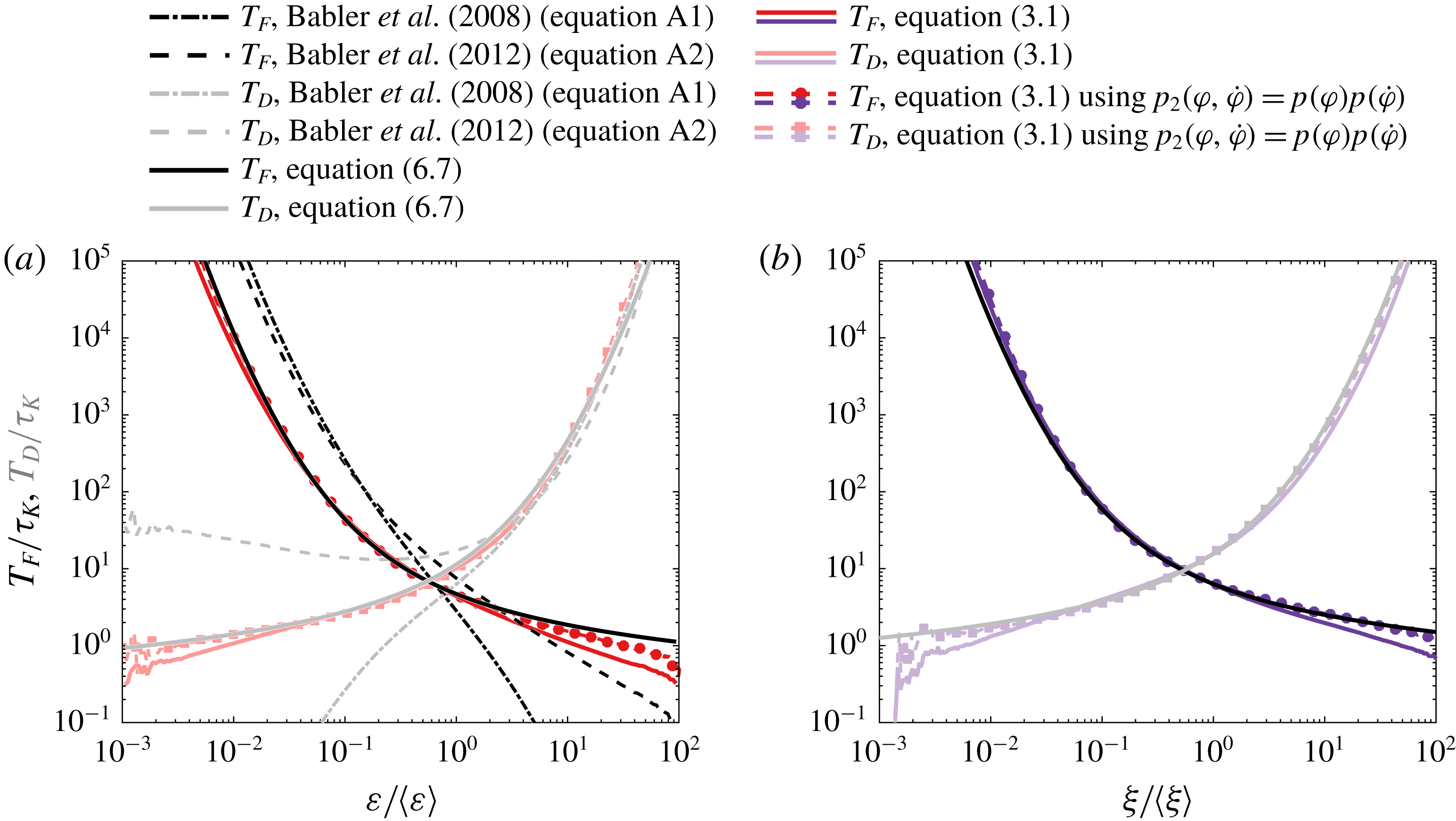
The mean times can also be inferred from the Rice theorem (Rice Reference Rice1945; Babler et al. Reference Babler, Biferale and Lanotte2012) described in the next section (equation (3.1)). This theorem uses distributions of the considered quantity and is therefore free of the influence of numerical temporal resolutions. Figure 3(d) compares mean flying and diving times obtained from the raw and extrapolated LPDFs and from the Rice theorem. While the aforementioned operation to clean and extrapolate the LPDFs may seem somewhat simplistic, it shows remarkable efficiency with good agreement between Lagrangian results and the Rice theorem.
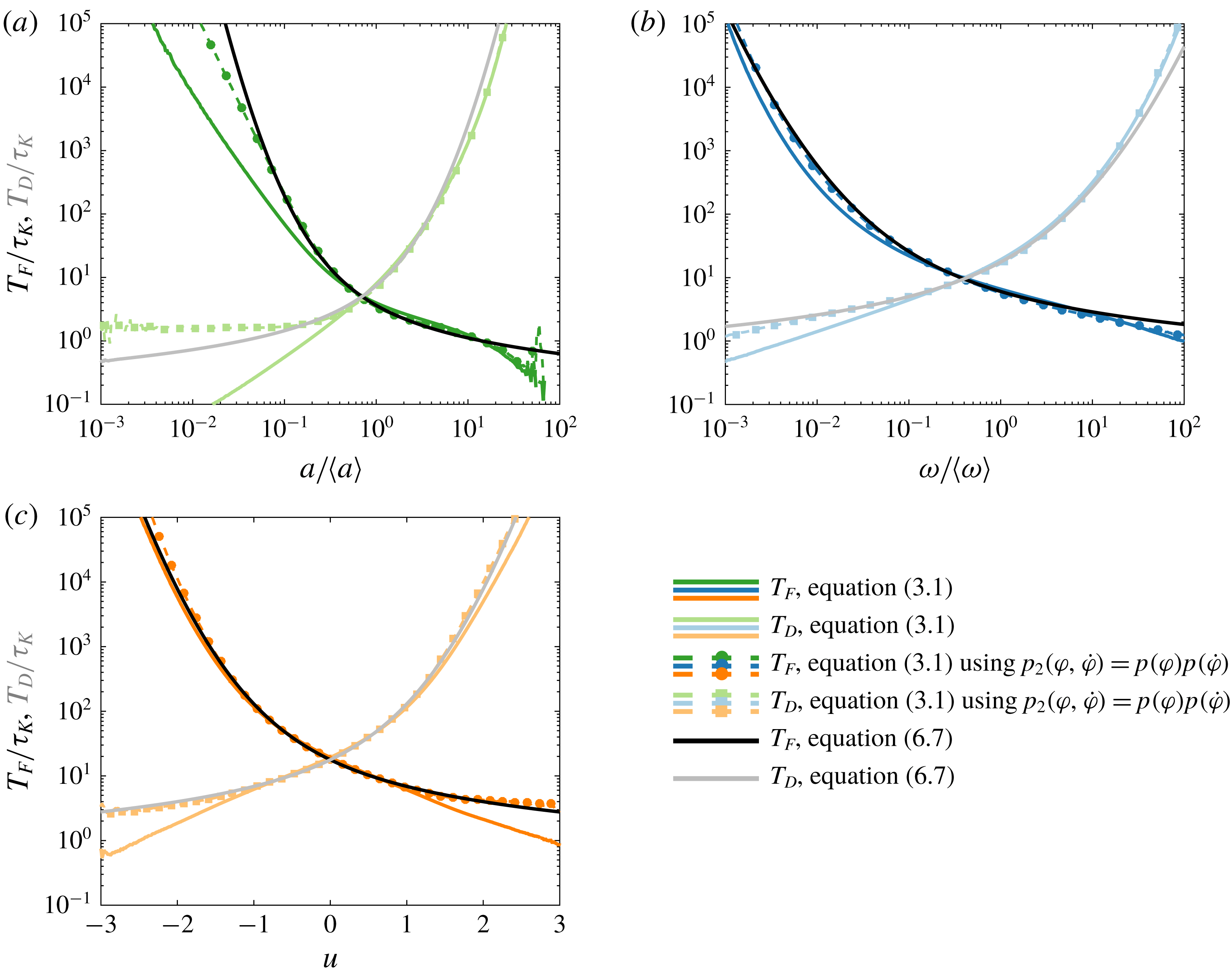
(a–c) Normalised mean flying and diving residence times,
 $T_{F}/\unicode[STIX]{x1D70F}_{K}$
and
 $T_{D}/\unicode[STIX]{x1D70F}_{K}$
, with respect to thresholds (a)
 $\unicode[STIX]{x1D700}_{t}/\langle \unicode[STIX]{x1D700}\rangle$
, (b)
 $a_{t}/\langle a\rangle$
and (c)
 $\unicode[STIX]{x1D714}_{t}/\langle \unicode[STIX]{x1D714}\rangle$
. Pure and lighter colours are flying and diving statistics, respectively. See encapsulated legend for details. The approximate global symmetry between
 $T_{F}$
and
 $T_{D}$
reflects the presence of holes, in contrast to bursts, during which magnitudes of at least one turbulent property can fall by several orders of magnitudes. Instead, local departure from this symmetry reflects a difference in the physics occurring during holes and bursts which characterises Lagrangian intermittency. Dashed black lines are the theoretical approximations (3.2) and (3.3).

3 Mean flying and diving times
 $T_{F}$
and
$T_{D}$


We first investigate the mean time scales of Lagrangian intermittency at various magnitudes of dissipation, acceleration and enstrophy. The mean flying and diving times
 $T_{F}(\unicode[STIX]{x1D711}_{t})$
and
 $T_{D}(\unicode[STIX]{x1D711}_{t})$
for the quantities
 $\unicode[STIX]{x1D711}=\unicode[STIX]{x1D700}$
,
 $a$
and
 $\unicode[STIX]{x1D714}$
are inferred using two different approaches: (i) from the integration of
 ${\mathcal{P}}_{\unicode[STIX]{x1D711}_{t}}^{F}(\ln \unicode[STIX]{x1D70F})$
and
 ${\mathcal{P}}_{\unicode[STIX]{x1D711}_{t}}^{D}(\ln \unicode[STIX]{x1D70F})$
, and (ii) from the Rice theorem defining the mean flying (diving) time as the ratio between the fraction of time spent above (below) the threshold
 $\unicode[STIX]{x1D711}_{t}$
and the mean time derivative
 $\dot{\unicode[STIX]{x1D711}}$
at
 $\unicode[STIX]{x1D711}_{t}$
, which in terms of distributions reads
 $$\begin{eqnarray}T_{F}(\unicode[STIX]{x1D711}_{t})={\displaystyle \frac{\displaystyle \int _{\unicode[STIX]{x1D711}_{t}}^{\infty }p(\unicode[STIX]{x1D711})\,\text{d}\unicode[STIX]{x1D711}}{\displaystyle \int _{0}^{\infty }\dot{\unicode[STIX]{x1D711}}p_{2}(\unicode[STIX]{x1D711}_{t},\dot{\unicode[STIX]{x1D711}})\,\text{d}\dot{\unicode[STIX]{x1D711}}}},\quad T_{D}(\unicode[STIX]{x1D711}_{t})={\displaystyle \frac{\displaystyle \int _{0}^{\unicode[STIX]{x1D711}_{t}}p(\unicode[STIX]{x1D711})\,\text{d}\unicode[STIX]{x1D711}}{\displaystyle \int _{0}^{\infty }\dot{\unicode[STIX]{x1D711}}p_{2}(\unicode[STIX]{x1D711}_{t},\dot{\unicode[STIX]{x1D711}})\,\text{d}\dot{\unicode[STIX]{x1D711}}}}.\end{eqnarray}$$
As already mentioned in the previous section, the Rice theorem quantifies more accurately the mean times for extreme thresholds since Lagrangian statistics suffer both from lack of data and discrepancies in the extrapolation method. Profiles of mean times obtained from Lagrangian statistics are in good agreement with those calculated with the Rice theorem (figure 4
a–c). For all three quantities, the profiles
 $T_{F}$
and
 $T_{D}$
exhibit a globally symmetrical behaviour on a log scale (figure 4
a–c). This entails two noteworthy characteristics of Lagrangian temporal statistics.
First, for all three quantities, the axis of symmetry, where
 $T_{F}=T_{D}$
, is located at a threshold
 $\unicode[STIX]{x1D711}_{t}^{s}$
which is different than the mean value
 $\langle \unicode[STIX]{x1D711}\rangle$
. Recalling that flying and diving LPDFs are transformation invariant, one can solve
 $T_{F}(\unicode[STIX]{x1D711}_{t}^{s})=T_{D}(\unicode[STIX]{x1D711}_{t}^{s})$
by considering the equality
 $T_{F}(\ln \unicode[STIX]{x1D711}_{t}^{s}/\langle \unicode[STIX]{x1D711}\rangle )=T_{D}(\ln \unicode[STIX]{x1D711}_{t}^{s}/\langle \unicode[STIX]{x1D711}\rangle )$
and approximating
 $\ln \unicode[STIX]{x1D711}/\langle \unicode[STIX]{x1D711}\rangle$
with a Gaussian distribution in (3.1), leading to
 $$\begin{eqnarray}\unicode[STIX]{x1D711}_{t}^{s}\approx \langle \unicode[STIX]{x1D711}\rangle \text{e}^{\langle \ln \unicode[STIX]{x1D711}/\langle \unicode[STIX]{x1D711}\rangle \rangle },\end{eqnarray}$$
and
 $\langle \ln \unicode[STIX]{x1D711}/\langle \unicode[STIX]{x1D711}\rangle \rangle \approx -\unicode[STIX]{x1D70E}_{\ln \unicode[STIX]{x1D711}}^{2}/2$
(Pope & Chen Reference Pope and Chen1990). The log-normal approximation is fairly accurate for
 $\unicode[STIX]{x1D711}=\unicode[STIX]{x1D700}$
and
 $\unicode[STIX]{x1D714}$
and acceptable for
 $a$
(figure 14) and (3.2) is verified for all three quantities with
 $\unicode[STIX]{x1D700}_{t}^{s}/\langle \unicode[STIX]{x1D700}\rangle \text{e}^{-\unicode[STIX]{x1D70E}_{\ln \unicode[STIX]{x1D700}}^{2}/2}=1.02$
,
 $\unicode[STIX]{x1D714}_{t}^{s}/\langle \unicode[STIX]{x1D714}\rangle \text{e}^{-\unicode[STIX]{x1D70E}_{\ln \unicode[STIX]{x1D714}}^{2}/2}=1.07$
and
 $a_{t}^{s}/\langle a\rangle \text{e}^{-\unicode[STIX]{x1D70E}_{\ln a}^{2}/2}=0.96$
. Hence, since
 $\unicode[STIX]{x1D711}_{t}^{s}$
can be well captured by the Gaussian approximation, it emerges from the multiplicative aspect of intermittency. Corresponding mean flying and diving times are approximately
 $T_{F|D}(\unicode[STIX]{x1D700}_{t}^{s})=7\unicode[STIX]{x1D70F}_{K}$
,
 $T_{F|D}(a_{t}^{s})=5\unicode[STIX]{x1D70F}_{K}$
and
 $T_{F|D}(\unicode[STIX]{x1D714}_{t}^{s})=10\unicode[STIX]{x1D70F}_{K}$
. These mean times are by construction equal to the inverse of the
 $\unicode[STIX]{x1D711}_{t}^{s}$
-crossing frequency,
 $1/N_{\unicode[STIX]{x1D711}_{t}^{s}}$
, hence, since
 $T_{F|D}(\unicode[STIX]{x1D711}_{t}^{s}/\langle \unicode[STIX]{x1D711}\rangle )=T_{F|D}(\ln \unicode[STIX]{x1D711}_{t}^{s}/\langle \unicode[STIX]{x1D711}\rangle )$
, one has
 $N_{\unicode[STIX]{x1D711}_{t}^{s}/\langle \unicode[STIX]{x1D711}\rangle }=N_{\ln \unicode[STIX]{x1D711}_{t}^{s}/\langle \unicode[STIX]{x1D711}\rangle }$
and, in the log-normal approximation, equation (1.2) considered in the Lagrangian framework tells that
 $$\begin{eqnarray}T_{F|D}(\unicode[STIX]{x1D711}_{t}^{s}/\langle \unicode[STIX]{x1D711}\rangle )\approx \unicode[STIX]{x03C0}\unicode[STIX]{x1D70F}_{L,\ln \unicode[STIX]{x1D711}},\end{eqnarray}$$
where
 $\unicode[STIX]{x1D70F}_{L,\ln \unicode[STIX]{x1D711}}$
is the Lagrangian Taylor time scale of
 $\ln \unicode[STIX]{x1D711}$
following (1.1). Results from of our simulation show that (3.3) is quite accurate for
 $\ln \unicode[STIX]{x1D700}$
and
 $\ln \unicode[STIX]{x1D714}$
, with
 $T_{F|D}(\unicode[STIX]{x1D700}_{t}^{s})/\unicode[STIX]{x03C0}\unicode[STIX]{x1D70F}_{L,\ln \unicode[STIX]{x1D700}}=1.1$
and
 $T_{F|D}(\unicode[STIX]{x1D714}_{t}^{s})/\unicode[STIX]{x03C0}\unicode[STIX]{x1D70F}_{L,\ln \unicode[STIX]{x1D714}}=1.2$
, respectively. On the contrary, the Taylor Lagrangian time scale of
 $\ln a$
is smaller than the mean residence time with
 $T_{F|D}(a_{t}^{s})/\unicode[STIX]{x03C0}\unicode[STIX]{x1D70F}_{L,\ln a}=1.4$
. Considering
 $\ln a$
as a Gaussian process is therefore accurate enough in order to infer
 $a_{t}^{s}$
but not to infer
 $\unicode[STIX]{x1D70F}_{L,\ln a}$
. However, this result may not be physical and may instead be explained by the known existing high-frequency spurious oscillations in
 $a$
at large magnitude (explaining the ‘bump’ in
 $T_{F}(a_{t})$
in figure 4
b) due to the integration scheme van Hinsberg et al. (Reference van Hinsberg, ten Thije Boonkkamp, Toschi and Clercx2013) which affect more
 $\unicode[STIX]{x1D70F}_{L,\ln a}$
due to the computed time derivative than
 $a_{t}^{s}$
. Note that by definition, for any threshold, the number of flying events,
 $N_{eF}$
, necessarily equals that of diving events,
 $N_{eF}=N_{eD}=N_{e}/2$
, hence, given that
 $N_{e}/2T_{F}+N_{e}/2T_{D}=T$
and that
 $T_{F}=T_{D}$
at
 $\unicode[STIX]{x1D711}_{t}^{s}$
, one has that the total flying and diving times are equal to half the total time,
 $N_{e}/2T_{F}=N_{e}/2T_{D}=T/2$
.
Second, the symmetry of the mean flying and diving times shows the existence in all three quantities of holes mirroring bursts, as previously suggested (Dubrulle Reference Dubrulle1994; She & Leveque Reference She and Leveque1994; She & Waymire Reference She and Waymire1995; Gledzer et al.
Reference Gledzer, Villermaux, Kahalerras and Gagne1996). Indeed, for periods where particles undergo bursts of large magnitudes, the existing symmetry dictates that there are periods of similar duration where particles undergo holes of small magnitudes. Profiles of
 $T_{F}$
and
 $T_{D}$
show that the time scales of holes are however slightly different than those of bursts. These differences are witness to Lagrangian intermittency, and can be better seen when superposing the profiles of mean diving times with those of flying times mirrored using
 $\unicode[STIX]{x1D711}_{t}^{s}$
as an axis of symmetry. For dissipation (figure 4
a), the mean time spent in holes is always larger than that spent in bursts (the dashed line is always above the solid line), and surprisingly, the mean diving time at large threshold, i.e. the time spent between bursts, is also always larger than the mean flying time at small threshold, i.e. the time spent between holes. Given that times spent in and between holes or bursts are complementary, such findings are only possible with an occurrence of holes higher than that of bursts, hence highlighting the different physics in play at small and large dissipation rates. For acceleration and enstrophy, comparison between profiles of
 $T_{F}$
and
 $T_{D}$
show that holes are shorter than bursts, hence highlighting here too Lagrangian intermittency, but their occurrence seem similar since times spent between holes are larger than times spent between bursts (figure 4
b,c).
4 The flying and diving LPDFs of turbulent quantities
4.1 The flying and diving LPDFs of dissipation at
$\unicode[STIX]{x1D700}_{t}^{s}$

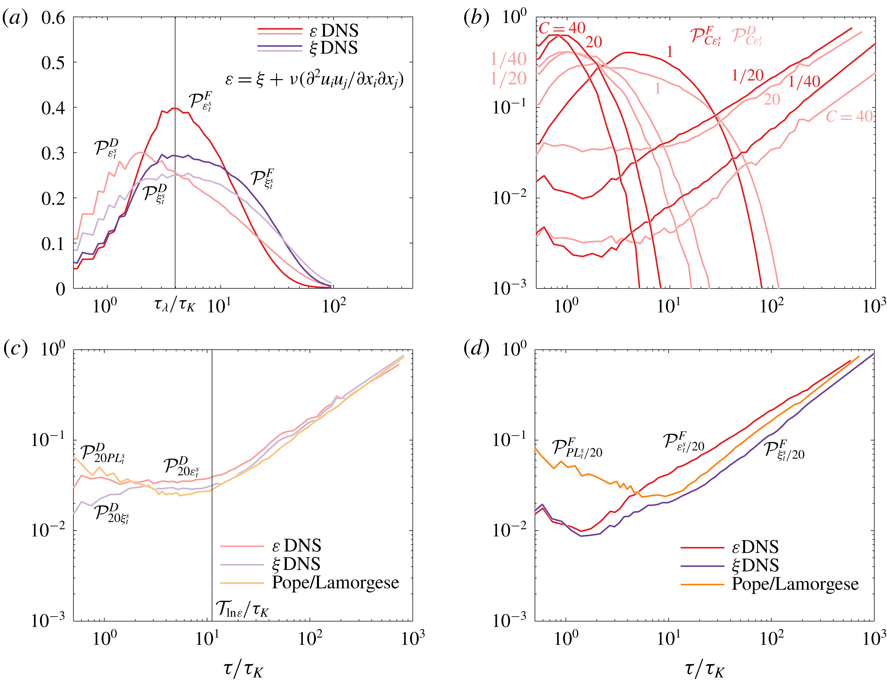
We first focus on the distributions of flights and dives of dissipation. Figure 5(a) shows the flying and diving LPDFs of
 $\unicode[STIX]{x1D700}$
at
 $\unicode[STIX]{x1D700}_{t}^{s}$
,
 ${\mathcal{P}}_{\unicode[STIX]{x1D700}_{t}^{s}}^{F}(\ln \unicode[STIX]{x1D70F})$
and
 ${\mathcal{P}}_{\unicode[STIX]{x1D700}_{t}^{s}}^{D}(\ln \unicode[STIX]{x1D70F})$
. A first result is that, although one has
 $T_{F}=T_{D}$
, the flying and diving LPDFs are not similar, showing once again the different dynamics governing flights and dives of a fluid parcel, even in HIT. Such asymmetry has already been detected in Eulerian statistics of turbulent boundary layers (Chamecki Reference Chamecki2013).
LPDFs
 ${\mathcal{P}}_{C\unicode[STIX]{x1D711}_{t}^{s}}^{F}$
(pure colours) and
 ${\mathcal{P}}_{C\unicode[STIX]{x1D711}_{t}^{s}}^{D}$
(lighter colours) of
 $\unicode[STIX]{x1D700}$
and
 $\unicode[STIX]{x1D709}$
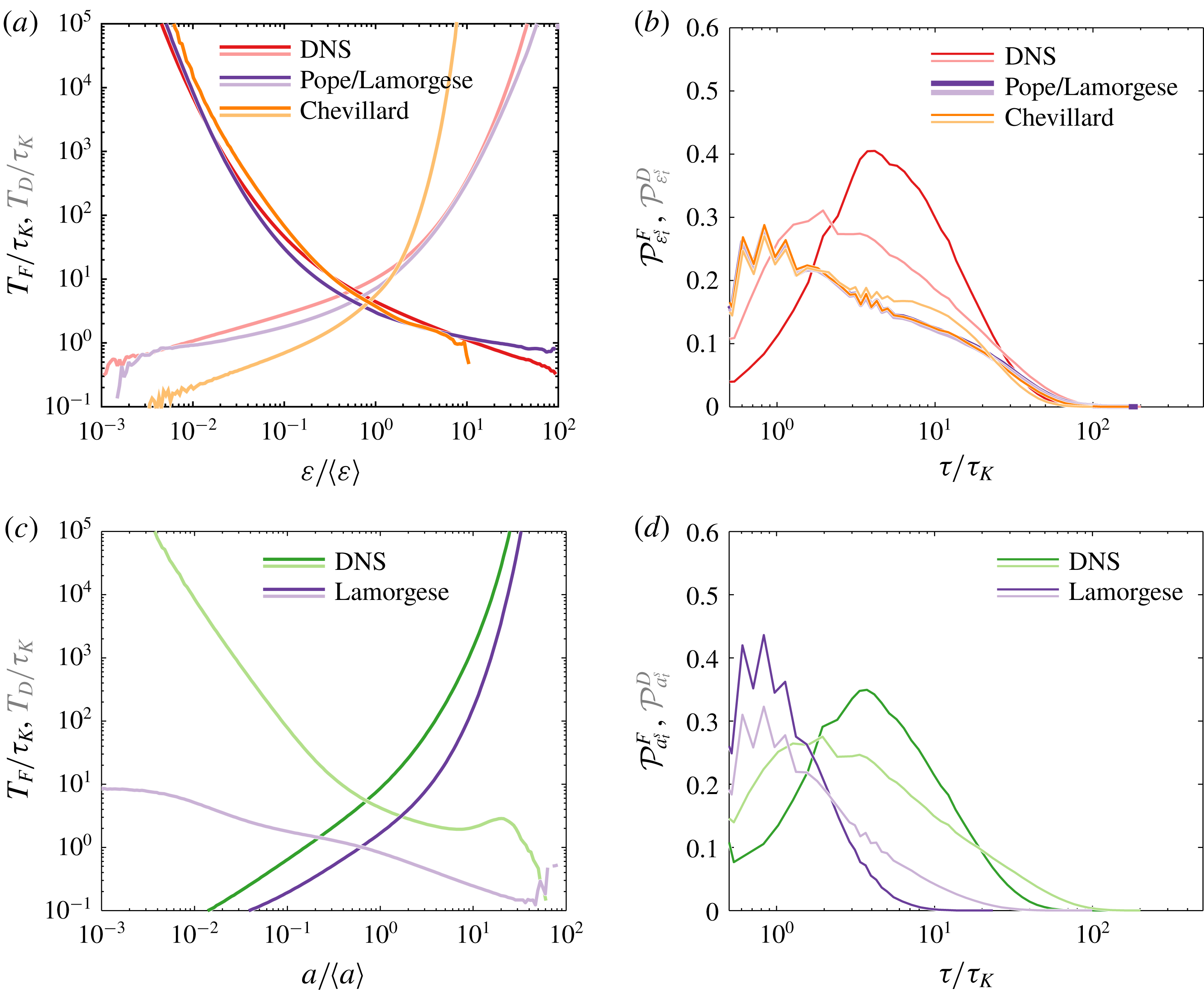
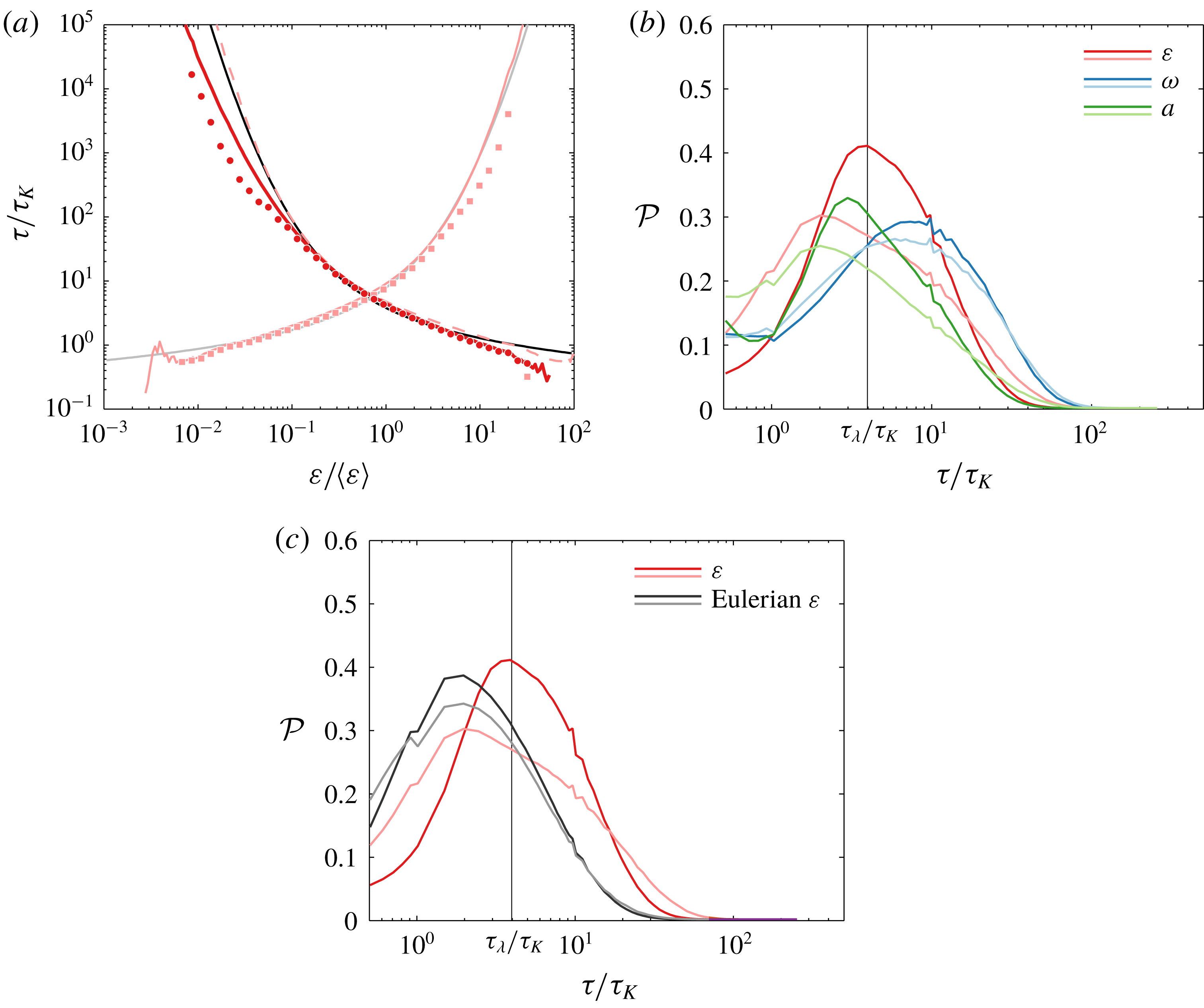
inferred from DNS and inferred from time series computed using the stochastic model of Pope & Chen (Reference Pope and Chen1990), Lamorgese et al. (Reference Lamorgese, Pope, Yeung and Sawford2007). (a) Results for
 $\unicode[STIX]{x1D700}$
and
 $\unicode[STIX]{x1D709}$
from DNS at threshold
 $\unicode[STIX]{x1D711}_{t}^{s}$
(
 $C=1$
). The different position of the peak in
 ${\mathcal{P}}_{\unicode[STIX]{x1D700}_{t}^{s}}^{F}$
and
 ${\mathcal{P}}_{\unicode[STIX]{x1D700}_{t}^{s}}^{D}$
is explained by the Reynolds stress. (b) LPDFs of
 $\unicode[STIX]{x1D700}$
for various values of
 $C$
. Flying and diving LPDFs can be paired following the approximate global symmetry with axis
 $\unicode[STIX]{x1D711}_{t}^{s}$
giving
 $T_{F}(C\unicode[STIX]{x1D711}_{t}^{s})\approx T_{D}(\unicode[STIX]{x1D711}_{t}^{s}/C)$
and
 $T_{D}(C\unicode[STIX]{x1D711}_{t}^{s})\approx T_{F}(\unicode[STIX]{x1D711}_{t}^{s}/C)$
. (c)
 ${\mathcal{P}}^{D}$
of
 $\unicode[STIX]{x1D700}$
,
 $\unicode[STIX]{x1D709}$
and the stochastic model for
 $C=20$
. (d)
 ${\mathcal{P}}^{F}$
of
 $\unicode[STIX]{x1D700}$
,
 $\unicode[STIX]{x1D709}$
and the stochastic model for
 $C=1/20$
. The emergence of a peak in the flying LPDFs of dissipation and acceleration at
 $\unicode[STIX]{x1D711}_{t}^{s}$
shows the existence of a characteristic flying time at about the Taylor time scale. The flying and diving LPDFs have two regimes. The first regime (flat for
 $\unicode[STIX]{x1D700}$
, increasing/flat for
 $\unicode[STIX]{x1D709}$
and decreasing for the model) at small time scales represents the correlated events of bursts and holes and the second corresponds to temporal statistics between uncorrelated events. Hence bursts in
 $\unicode[STIX]{x1D700}$
and
 $\unicode[STIX]{x1D709}$
are events mostly correlated over their respective global decorrelation time scale
 ${\mathcal{T}}_{\ln \unicode[STIX]{x1D700}}$
and
 ${\mathcal{T}}_{\ln \unicode[STIX]{x1D709}}$
while holes are shorter events over a few
 $\unicode[STIX]{x1D70F}_{K}$
.

Both flying and diving LPDFs of dissipation exhibit a peak with a most probable flying time of approximately
 $4\unicode[STIX]{x1D70F}_{K}$
and a most probable diving time of approximately
 $2\unicode[STIX]{x1D70F}_{K}$
. A probability of having either short or long dives higher than that of having short or long flights explains why mean flying and diving times are equal despite a different most probable residence time. Importantly, the most probable flying time of
 $\unicode[STIX]{x1D700}$
at
 $\unicode[STIX]{x1D700}_{t}^{s}$
coincides with the Eulerian Taylor time scale, equal to
 $\unicode[STIX]{x1D70F}_{\unicode[STIX]{x1D706}}=\langle (\unicode[STIX]{x2202}u/\unicode[STIX]{x2202}x)^{2}\rangle ^{-1/2}=\sqrt{15}\unicode[STIX]{x1D70F}_{K}$
in HIT (Pope Reference Pope2000). Such a result is confirmed with the low Reynolds number simulation at
 $Re_{\unicode[STIX]{x1D706}}=90$
(see appendix D). On the contrary, neither time scale
 $\unicode[STIX]{x1D70F}_{L,\unicode[STIX]{x1D700}}=1.4\unicode[STIX]{x1D70F}_{K}$
nor
 $T_{F}(\unicode[STIX]{x1D700}_{t}^{s})\approx \unicode[STIX]{x03C0}\unicode[STIX]{x1D70F}_{L,\ln \unicode[STIX]{x1D700}}\approx 7\unicode[STIX]{x1D70F}_{K}$
represent any particular characteristic time of
 ${\mathcal{P}}_{\unicode[STIX]{x1D700}_{t}^{s}}^{F}$
(figure 5
a). Thus, the time scale
 $\unicode[STIX]{x1D70F}_{\unicode[STIX]{x1D706}}$
associated with the Eulerian vortices in the inertial cascade seems to be a good estimator for a wide range of
 $Re_{\unicode[STIX]{x1D706}}$
of the Lagrangian most probable flying residence time of dissipation above
 $\unicode[STIX]{x1D700}_{t}^{s}$
. Instead, numerical results (confirmed theoretically below in § 6) show that the mean flying and diving times at
 $\unicode[STIX]{x1D700}_{t}^{s}$
do not scale with
 $\unicode[STIX]{x1D70F}_{\unicode[STIX]{x1D706}}$
(i.e.
 $\unicode[STIX]{x1D70F}_{\unicode[STIX]{x1D706}}/T_{F|D}(\unicode[STIX]{x1D700}_{t}^{s})$
is Reynolds dependent). This suggests that while the peak of the flying LPDFs only emerges from the physics behind the inertial cascade (characterised by
 $\unicode[STIX]{x1D70F}_{\unicode[STIX]{x1D706}}$
), the mean flying and diving times instead also encompass the complex physics behind Lagrangian intermittency.
Interestingly, the flying LPDF of the pseudo-dissipation, a field usually considered in Lagrangian stochastic models instead of the dissipation rate as it has more favourable statistical properties such as Gaussianity, e.g. (Pope & Chen Reference Pope and Chen1990; Sawford Reference Sawford1991; Lamorgese et al.
Reference Lamorgese, Pope, Yeung and Sawford2007) and derived as
 $\unicode[STIX]{x1D709}=\unicode[STIX]{x1D700}-\unicode[STIX]{x1D708}\unicode[STIX]{x2202}_{i}\unicode[STIX]{x2202}_{j}u_{i}u_{j}$
(where
 $u_{i}u_{j}$
is the Reynolds stress which accounts for turbulent fluctuations in the flow), exhibits at
 $\unicode[STIX]{x1D709}_{t}^{s}$
a less prominent most probable residence time at
 $\unicode[STIX]{x1D70F}_{\unicode[STIX]{x1D706}}$
(figure 5
a). Moreover, the difference in most probable time scale between flying and diving LPDFs has vanished in the statistics of
 $\unicode[STIX]{x1D709}$
, with diving times of
 $\unicode[STIX]{x1D709}$
also equal to
 $\unicode[STIX]{x1D70F}_{\unicode[STIX]{x1D706}}$
. This result shows that Lagrangian fluctuations of the Reynolds stress (represented by the term
 $\unicode[STIX]{x2202}_{i}\unicode[STIX]{x2202}_{j}u_{i}u_{j}$
) play a key role in breaking the symmetry between flights and dives. Surprisingly, comparison between the statistics of
 $\unicode[STIX]{x1D700}$
and
 $\unicode[STIX]{x1D709}$
shows that the Reynolds stress only influences the time associated with the most probable diving time.
4.2 Insights into dissipation bursts
As the threshold is increased beyond
 $\unicode[STIX]{x1D700}_{t}^{s}$
, one gradually sees appearing the signature of dissipation bursts in the LPDFs. Figure 5(b) shows
 ${\mathcal{P}}_{\unicode[STIX]{x1D700}_{t}}^{F}$
and
 ${\mathcal{P}}_{\unicode[STIX]{x1D700}_{t}}^{D}$
for various thresholds
 $\unicode[STIX]{x1D700}_{t}^{s}/C$
and
 $C\unicode[STIX]{x1D700}_{t}^{s}$
with
 $C=1/40$
,
 $1/20$
,
 $1$
,
 $20$
and
 $40$
. Note that due to the symmetry at
 $\unicode[STIX]{x1D700}_{t}^{s}$
, one has
 $T_{F}(C\unicode[STIX]{x1D700}_{t}^{s})\approx T_{D}(\unicode[STIX]{x1D700}_{t}^{s}/C)$
and
 $T_{D}(C\unicode[STIX]{x1D700}_{t}^{s})\approx T_{F}(\unicode[STIX]{x1D700}_{t}^{s}/C)$
(although the latter is less accurate as can be seen in figure 4
a). The impact of bursts is prominent on the flying LPDF at large threshold,
 ${\mathcal{P}}_{20\unicode[STIX]{x1D700}_{t}^{s}}^{F}$
. The most probable flying time is smaller, showing the overall brevity of bursts. The density of the most probable time has increased and, consequently, the range of possible flying times has decreased. Yet, even for a threshold ten times larger than the mean dissipation (equivalent to
 $20\unicode[STIX]{x1D711}_{t}^{s}$
), particles can sometimes undergo a strong shear for up to
 $15\unicode[STIX]{x1D70F}_{K}$
(at a density of approximately
 $10^{-5}$
, not shown here). For a larger threshold (
 $C=40$
), the most probable flying time is slightly smaller but, interestingly, neither the corresponding density nor the variance changes much. Only the maximum flying time available decreases. It is worth noting that the peak of the LPDFs occurs at about the Kolmogorov time scale, however, this time scale cannot be considered here as a relevant physical time scale to describe these LPDFs since the local dissipation is much greater than the mean dissipation used to determine
 $\unicode[STIX]{x1D70F}_{K}$
.
The diving LPDFs at large thresholds,
 ${\mathcal{P}}_{20\unicode[STIX]{x1D700}_{t}^{s}}^{D}$
and
 ${\mathcal{P}}_{40\unicode[STIX]{x1D700}_{t}^{s}}^{D}$
(figure 5
b in light red) also bear information on the physics of bursts. Indeed, at small residence times, dives are brief and can therefore belong to one specific event of burst (figure 1). One can see that the diving LPDFs have two different regimes with the first being a constant density for dives of up to
 $10\unicode[STIX]{x1D70F}_{K}$
and the second being a linearly increasing density with slope unity. Interestingly, pseudo-dissipation
 $\unicode[STIX]{x1D709}$
has the same temporal statistics except in the first regime, where density is smaller for diving times below
 $2\unicode[STIX]{x1D70F}_{K}$
, thus showing that the Reynolds stress adds more small-scale variations during dives in bursts of Lagrangian dissipation (figure 5
c), and potentially explaining the shift of the diving LPDFs at
 $\unicode[STIX]{x1D711}_{t}^{s}$
(figure 5
a). Using the Lagrangian stochastic model of dissipation (Pope & Chen Reference Pope and Chen1990; Lamorgese et al.
Reference Lamorgese, Pope, Yeung and Sawford2007) based on a first-order autoregressive model, we produced a set of time series and derived from it the flying and diving LPDFs (see appendix C). Diving LPDFs at large threshold also exhibit two regimes separated at approximately
 $10\unicode[STIX]{x1D70F}_{K}$
(figure 5
c). The corresponding change in regime can only be dictated by the time scale prescribed to the model, namely, the decorrelation time scale of the order of magnitude of the dissipation,
 ${\mathcal{T}}_{\ln \unicode[STIX]{x1D700}}\approx 12\unicode[STIX]{x1D70F}_{K}$
. Our results show that the first regime in temporal statistics of dissipation at large threshold is governed by the correlated fluctuations of dissipation, in part due to Reynolds stress. These correlated fluctuations reflect an ongoing burst. Hence, the diving LPDF at large threshold represents an interesting manner to detect the decorrelation time scale of a burst. The combination of results on the statistics of flights and dives at large threshold shows that, in Lagrangian turbulent dissipation, bursts are events likely to happen over approximately
 ${\mathcal{T}}_{\ln \unicode[STIX]{x1D700}}$
with small-scale fluctuations composed of flying periods mainly taking place over
 $\unicode[STIX]{x1D70F}_{K}$
and diving periods equally occurring over times from one to
 ${\mathcal{T}}_{\ln \unicode[STIX]{x1D700}}$
.
The second regime present in
 ${\mathcal{P}}_{\unicode[STIX]{x1D700}_{t}}^{D}$
at large threshold shows the probability of the time delay between two uncorrelated events and therefore tells us about the frequency of the bursts. The most probable time period between two bursts is of several hundreds of
 $\unicode[STIX]{x1D70F}_{K}$
(figure 5
b), showing that in a turbulent flow, extreme events have such a low occurrence that, should the event of turbulence in a flow be finite in time, bursts would not be undergone by most particles.
4.3 Insights into dissipation holes
At small threshold, statistics of residence times are mostly dictated by the realm of holes (figure 1). Equivalently to results on bursts, the most probable diving time in
 ${\mathcal{P}}_{\unicode[STIX]{x1D700}_{t}^{s}/20}^{D}$
and
 ${\mathcal{P}}_{\unicode[STIX]{x1D700}_{t}^{s}/40}^{D}$
has also decreased down to small time scales as well as the variance of the distribution (figure 5
b). Here too, despite the extreme context, the particle can sometime undergo long quiet events for periods up to
 $35\unicode[STIX]{x1D70F}_{K}$
(at a density of approximately
 $10^{-5}$
, not shown here). However, differences exist with respect to the flying LPDFs at large threshold,
 ${\mathcal{P}}_{20\unicode[STIX]{x1D700}_{t}^{s}}^{F}$
and
 ${\mathcal{P}}_{40\unicode[STIX]{x1D700}_{t}^{s}}^{F}$
, which explain the slight break of symmetry between bursts and holes (figure 4
a).
First, the most probable time of the LPDFs is less clearly defined and the variance of the distribution is larger than that of flying times at large threshold, reflecting a larger range of possible diving times. Second, as for bursts at large threshold, events of holes below threshold
 $\unicode[STIX]{x1D700}_{t}^{s}/20$
are predominantly occurring on a small time scale, however,
 ${\mathcal{P}}_{\unicode[STIX]{x1D700}_{t}^{s}/20}^{F}$
does not exhibit the same two regimes as in
 ${\mathcal{P}}_{20\unicode[STIX]{x1D700}_{t}^{s}}^{D}$
. The first regime of
 ${\mathcal{P}}_{\unicode[STIX]{x1D700}_{t}^{s}/20}^{F}$
consists of a decrease of probability as the residence time increases, and a second regime of linearly increasing probability starting at approximately
 $2\unicode[STIX]{x1D70F}_{K}$
(figure 5
b, red curve). This holds true also for larger thresholds (
 $C=40$
). As for
 ${\mathcal{P}}_{20\unicode[STIX]{x1D700}_{t}^{s}}^{D}$
, the second linear regime in
 ${\mathcal{P}}_{\unicode[STIX]{x1D700}_{t}^{s}/20}^{F}$
is witness to dives between two uncorrelated events of holes and therefore shows that two holes are most likely to be separated by periods more than two orders of magnitude above
 $\unicode[STIX]{x1D70F}_{K}$
(figure 5
b).
The brevity of the first regime corresponding to the statistics of correlated events tells us that events of holes are likely to happen in one shot over small time scales of a few
 $\unicode[STIX]{x1D70F}_{K}$
instead of the global decorrelation time scale. Here,
 ${\mathcal{P}}_{\unicode[STIX]{x1D709}_{t}^{s}/20}^{F}$
behaves like
 ${\mathcal{P}}_{\unicode[STIX]{x1D700}_{t}^{s}/20}^{F}$
(figure 5
d), which is logically explained by the fact that, at small threshold, the corresponding Reynolds stress is small and therefore weakly influential.
Finally, the stochastic model (6.1) used here (Pope & Chen Reference Pope and Chen1990; Lamorgese et al.
Reference Lamorgese, Pope, Yeung and Sawford2007) could not reproduce the flying LPDFs at large threshold (figure 5
d). This is explained by the fact that the model necessarily generates a signal continuously correlated over
 ${\mathcal{T}}_{\ln \unicode[STIX]{x1D700}}$
. Such a result shows that, in turbulence, the length of memory in time of Lagrangian physics is event dependent and therefore varies across the flow. While holes belong to a physics occurring with a memory over
 ${\sim}2\unicode[STIX]{x1D70F}_{K}$
, bursts happen over the large scale
 ${\mathcal{T}}_{\ln \unicode[STIX]{x1D700}}$
.
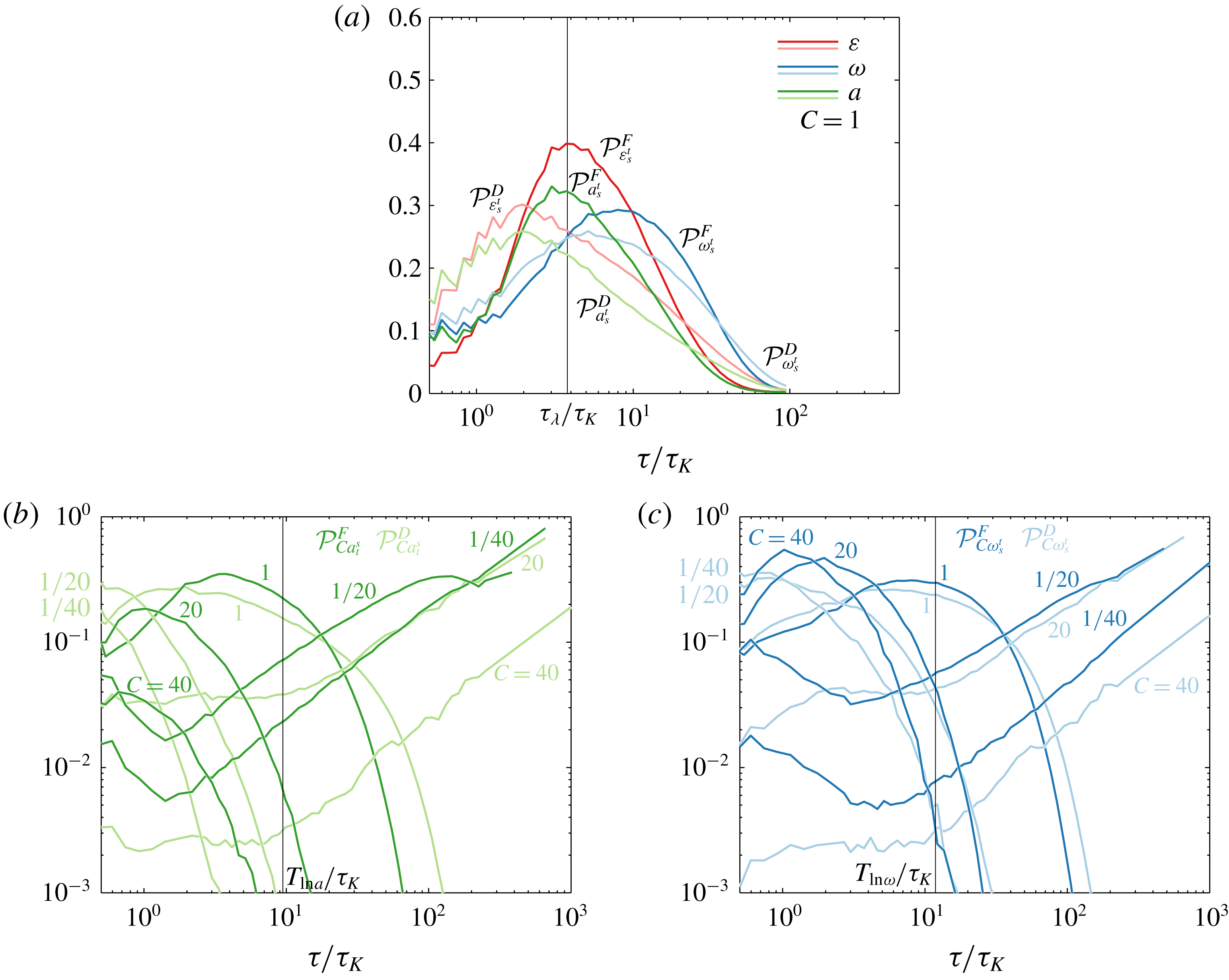
(a) Flying (pure colours) and diving (lighter colours) LPDFs of dissipation, acceleration and enstrophy at their respective
 $\unicode[STIX]{x1D700}_{t}^{s}$
,
 $a_{t}^{s}$
and
 $\unicode[STIX]{x1D714}_{t}^{s}$
. As for dissipation, the most probable flying time of acceleration at
 $a_{t}^{s}$
is
 $\unicode[STIX]{x1D70F}_{\unicode[STIX]{x1D706}}$
. It is instead twice as large for
 $\unicode[STIX]{x1D714}$
. (b,c) Flying and diving LPDFs for various values of
 $C$
as in figure 5. Diving LPDFs of both acceleration and enstrophy at large magnitude exhibit two regimes that can be delimited by their respective decorrelation time scale.

4.4 The flying and diving LPDFs of acceleration and enstrophy
Results of temporal statistics of acceleration and enstrophy are globally equivalent to those of dissipation, showing the presence of bursts and holes in these properties as well. For both flying and diving times, statistics of acceleration at
 $a_{t}^{s}$
have equivalent flying and diving LPDFs as those of dissipation (figure 6
a) and also exhibit two regimes of dives and flights at large and small threshold respectively revealing the presence of bursts and holes of acceleration (figure 6
b). Such similarity with the statistics of dissipation corroborates the presumed link between intermittency of dissipation and acceleration (Lamorgese et al.
Reference Lamorgese, Pope, Yeung and Sawford2007). However, one can see that the amplitude of the fluctuations in acceleration seems more constrained and flights above
 $40a_{t}^{s}$
are rare, inducing small densities of the corresponding LPDFs in the observed range of time travel (figure 5
b). Moreover, while the peak of
 ${\mathcal{P}}_{a_{t}^{s}}^{F}$
is located at
 $\unicode[STIX]{x1D70F}_{\unicode[STIX]{x1D706}}$
in the case
 $Re_{\unicode[STIX]{x1D706}}=240$
, it is located at a smaller time in the low Reynolds number simulation (
 $Re_{\unicode[STIX]{x1D706}}=90$
), hence showing a different dependency on
 $Re_{\unicode[STIX]{x1D706}}$
than for dissipation (figure 16
b). It is therefore not possible to conclude at this stage whether
 $\unicode[STIX]{x1D70F}_{\unicode[STIX]{x1D706}}$
is a time scale of convergence for acceleration.
Instead, the statistics of enstrophy have a few differences with respect to dissipation and acceleration. The most probable flying time for enstrophy at
 $\unicode[STIX]{x1D714}_{t}^{s}$
is approximately
 $10\unicode[STIX]{x1D70F}_{K}$
(figure 6
a), showing that fluctuations of the rate-of-rotation are slower than that of the rate-of-strain. Moreover, the asymmetry between flights and dives is weaker (figure 6
a). The diving LPDFs at small thresholds (
 ${\mathcal{P}}_{\unicode[STIX]{x1D714}_{t}^{s}/20}^{F}$
and
 ${\mathcal{P}}_{\unicode[STIX]{x1D714}_{t}^{s}/40}^{F}$
) show that holes of enstrophy last longer up to
 $5\unicode[STIX]{x1D70F}_{K}$
while the flying LPDFs at large thresholds show that a particle can travel for a long period of time (i.e. few tens of
 $\unicode[STIX]{x1D70F}_{K}$
) across highly enstrophic regions (figure 6
c). Finally, for both acceleration and enstrophy, the first regime is defined up to a time scale consistent with
 ${\mathcal{T}}_{\ln a}\approx 9.5\unicode[STIX]{x1D70F}_{K}$
and
 ${\mathcal{T}}_{\ln \unicode[STIX]{x1D714}}\approx 12\unicode[STIX]{x1D70F}_{K}$
, respectively.
5 Flow structure characteristics during Lagrangian bursts and holes
In a turbulent flow, fluid particles travel across various flow structures which are believed to be a cornerstone of turbulence formation (Chong, Perry & Cantwell Reference Chong, Perry and Cantwell1990; Meneveau Reference Meneveau2011). The understanding of these geometries has significantly increased in the past decades (Chong et al. Reference Chong, Perry and Cantwell1990; Cantwell Reference Cantwell1993; Perry & Chong Reference Perry and Chong1994; Soria et al. Reference Soria, Sondergaard, Cantwell, Chong and Perry1994; Martin et al. Reference Martin, Ooi, Chong and Soria1998; Ooi et al. Reference Ooi, Martin, Soria and Chong1999; Wang et al. Reference Wang, Bergstrom, Yin and Yee2006; da Silva & Pereira Reference da Silva and Pereira2008; Meneveau Reference Meneveau2011). In this section, we study whether events of Lagrangian bursts and holes are linked to specific characteristics of the local Eulerian structure of the flow.
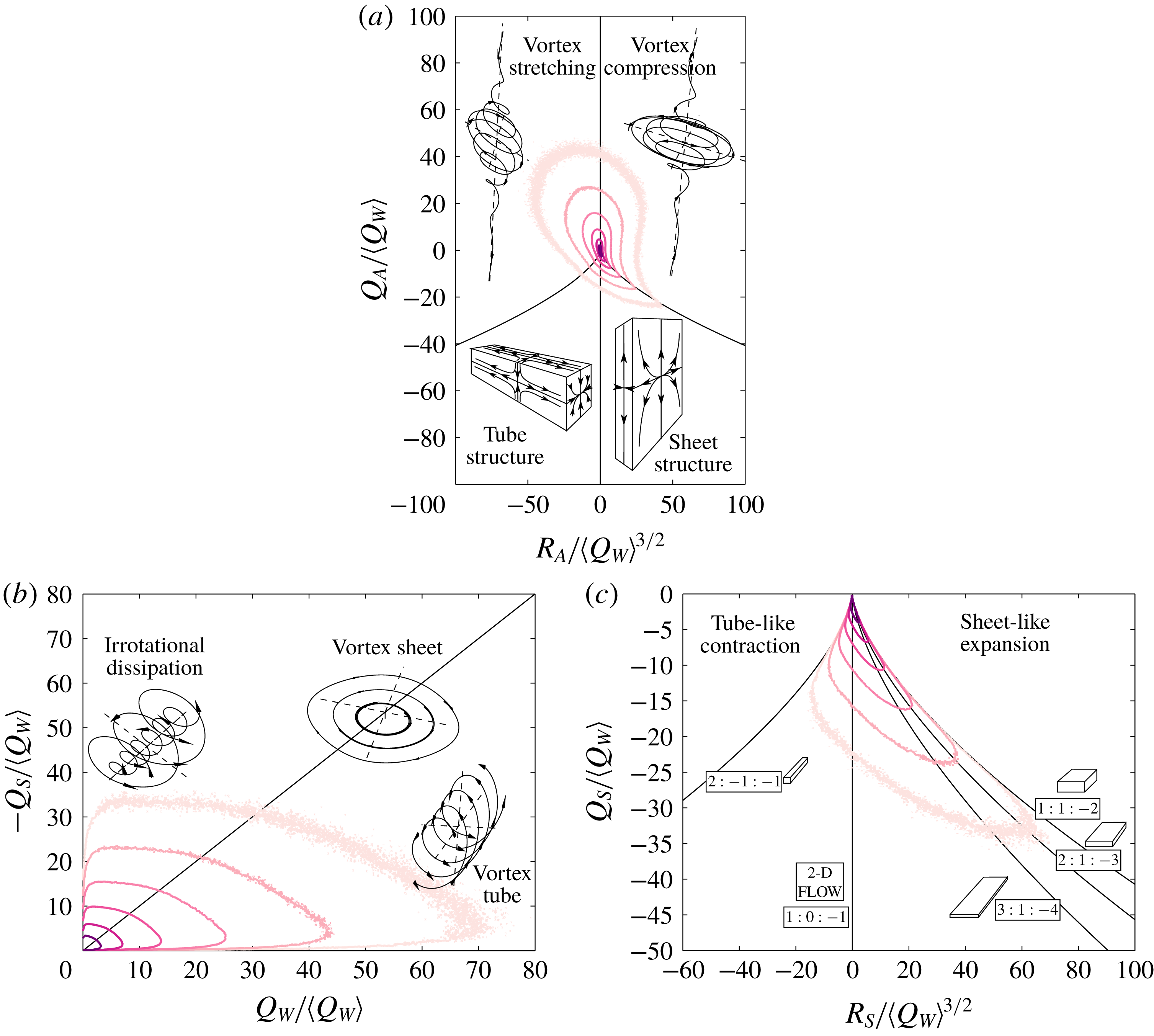
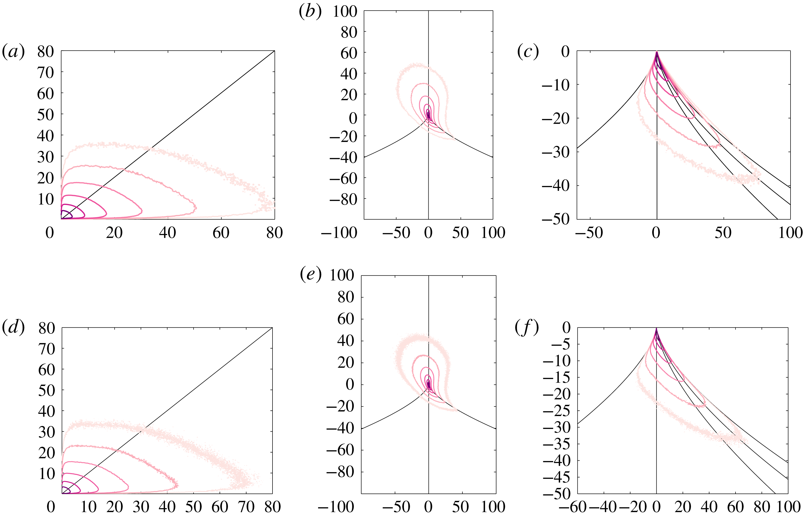
Flow geometries associated with the joint distributions of the velocity gradient invariants (a) (
 $Q_{A}$
,
 $R_{A}$
), (b) (
 $-Q_{S},Q_{W}$
) and (c)
 $(Q_{S},R_{S})$
. The invariants are normalised by
 $\langle Q_{W}\rangle$
. Results are consistent with previous studies (Martin et al.
Reference Martin, Ooi, Chong and Soria1998; Ooi et al.
Reference Ooi, Martin, Soria and Chong1999) and show that in HIT, there is a preference for stretching vortices and sheet-like straining expansions.

5.1 The various structures of HIT
The velocity field surrounding a fluid parcel is quantified by the velocity gradient tensor
 $\unicode[STIX]{x1D608}_{ij}$
, which encodes information about the first-order near-future directions taken by the parcel. In turbulence, this information holds for a time of the order of the local viscous time scale
 $\unicode[STIX]{x1D70F}_{K}(\unicode[STIX]{x1D700})=(\unicode[STIX]{x1D708}/\unicode[STIX]{x1D700}^{3})^{1/4}$
(Meneveau Reference Meneveau2011). The eigenvectors and eigenvalues of
 $\unicode[STIX]{x1D608}_{ij}$
define the principal directions and magnitudes of influence of velocity gradients, respectively. Each eigenvalue of
 $\unicode[STIX]{x1D608}_{ij}$
satisfies a characteristic equation whose coefficients
 $Q_{A}$
and
 $R_{A}$
are the velocity invariants and indicate whether the fluid parcel is in a vortex or straining structure predominantly stretching or compressing the flow (figure 7
b). Similarly, the study of the non-zero invariants of the tensors of rate-of-strain,
 $\unicode[STIX]{x1D61A}_{ij}$
, and the rate-of-rotation,
 $\unicode[STIX]{x1D61E}_{ij}$
, namely
 $Q_{S}$
,
 $R_{S}$
and
 $Q_{W}$
, indicate the strain and rotation configuration of the flow structure (figure 7
a,c). Invariants
 $Q_{S}$
and
 $Q_{W}$
are directly related to dissipation and enstrophy such that
 $Q_{S}/\langle Q_{W}\rangle =-\unicode[STIX]{x1D700}/\langle \unicode[STIX]{x1D700}\rangle$
and
 $Q_{W}/\langle Q_{W}\rangle =\unicode[STIX]{x1D714}/\langle \unicode[STIX]{x1D714}\rangle$
. Details on the theoretical background linking the invariants and the flow geometries in the context of HIT are given in appendix B. Thus, the set of five invariants (
 $Q_{S}$
,
 $Q_{W}$
,
 $R_{S}$
,
 $Q_{A}$
and
 $R_{A}$
) represents a first-order description of the local flow structures. Specifically, the study of the joint distributions (
 $Q_{W}$
,
 $Q_{S}$
), (
 $R_{S}$
,
 $Q_{S}$
) and (
 $R_{A}$
,
 $Q_{A}$
) tells whether the particle is within a straining or vortical, and stretching or compressive flow structure (figure 7).
Total joint distributions of invariants obtained with our DNS (figure 7; see appendix B for details) resemble those of previous studies (Soria et al.
Reference Soria, Sondergaard, Cantwell, Chong and Perry1994; Martin et al.
Reference Martin, Ooi, Chong and Soria1998; Ooi et al.
Reference Ooi, Martin, Soria and Chong1999). The joint distribution of (
 $Q_{A}$
,
 $R_{A}$
) has a teardrop shape highlighting the predominance of vortices and sheet-like structures in the flow. It has been shown (Martin et al.
Reference Martin, Ooi, Chong and Soria1998) that, in homogeneous isotropic turbulence, a fluid parcel spends approximately 20 % of the time as part of a vortex stretching flow structure, 20 % of the time as a vortex compressing topology, more than half the time as a sheet-like straining structure and, finally, the remaining time as a tube-like straining structure (figure 7
b). Instead, irrotational dissipations, vortex sheets and vortex tubes have a somewhat equal chance of existing in the flow (figure 7
a). Statistics of residence time in each region tend to follow exponentially decaying tails (Bhatnagar et al.
Reference Bhatnagar, Gupta, Mitra, Pandit and Perlekar2016). The slight inclination toward the axis of
 $Q_{W}$
suggests that highly enstrophic geometries occur with small straining and are possibly long lived (Ooi et al.
Reference Ooi, Martin, Soria and Chong1999). Finally, configurations of rate-of-strain can be differentiated with the parameter
 $s^{\star }=-3\sqrt{6}\unicode[STIX]{x1D6FC}_{S}\unicode[STIX]{x1D6FD}_{S}\unicode[STIX]{x1D6FE}_{S}/(\unicode[STIX]{x1D6FC}_{S}^{2}+\unicode[STIX]{x1D6FD}_{S}^{2}+\unicode[STIX]{x1D6FE}_{S}^{2})^{3/2}$
(Lund & Rogers Reference Lund and Rogers1994), where
 $\unicode[STIX]{x1D6FC}_{S},\unicode[STIX]{x1D6FD}_{S}$
and
 $\unicode[STIX]{x1D6FE}_{S}$
are the principal strain rates of
 $\unicode[STIX]{x1D61A}_{ij}$
(see appendix B). Isolines of
 $s^{\star }$
are drawn in the distribution (
 $Q_{S}$
,
 $R_{S}$
) (figure 7
c). Our results show that the preferred straining geometry at large rate of strain is a sheet-like structure with a configuration
 $\unicode[STIX]{x1D6FC}_{S}:\unicode[STIX]{x1D6FD}_{S}:\unicode[STIX]{x1D6FE}_{S}=2:1:-3$
(figure 7
a). Note that although this preferred configuration is different than that found in the first studies on this topic (Ashurst et al.
Reference Ashurst, Kerstein, Kerr and Gibson1987; Lund & Rogers Reference Lund and Rogers1994) i.e.
 $3:1:-4$
, it is consistent with more recent work (Ooi et al.
Reference Ooi, Martin, Soria and Chong1999). As the Reynolds number of the simulations conducted in these aforementioned studies was similar, the difference in small-scale configuration could be imputed to different initial and forcing configurations as already suggested (Soria et al.
Reference Soria, Sondergaard, Cantwell, Chong and Perry1994).
Normalised joint distributions of the velocity gradient invariants during bursts (main figure) and holes (inset) using (a–c)
 $X=Q_{W}/\langle Q_{W}\rangle ,Y=-Q_{S}/\langle Q_{W}\rangle$
, (d–f)
 $R_{A}/\langle Q_{W}\rangle ^{3/2},Q_{A}/\langle Q_{W}\rangle$
and (g–i)
 $R_{S}/\langle Q_{W}\rangle ^{3/2},Q_{S}/\langle Q_{W}\rangle$
for (a,d,g) dissipation (
 $C=20$
and
 $C=1/10$
), (b,e,h) acceleration (
 $C=10$
and
 $C=1/5$
) and (c,f,i) enstrophy (
 $C=20$
and
 $C=1/10$
). Black, pure colour, grey and lighter colour distributions are obtained by considering invariants at initial time of flights, times of maximum magnitude during flights, initial time of dives and times of minimum magnitude during dives, respectively (represented in figure 1). Distributions are inferred by only considering flights and dives of less than
 $3\unicode[STIX]{x1D70F}_{K}$
, hence capturing bursts events (large
 $C$
) and holes (small
 $C$
). Each joint distribution is normalised by the maximum density and isolines
 $0.90$
and
 $0.05$
are shown here. (a–c) In contrast to the global distributions shown in figure 7(b), bursts of dissipation and acceleration occur mainly in irrotational structures. Flights and dives of enstrophy are often correlated with an increase and decrease of
 $Q_{S}$
. The joint distributions are globally self-similar. (d–f) For dissipation and acceleration, there are no preferred structures relative to those in HIT (figure 7
a). Dives tend however to equally happen in stretching and compressing vortices. Finally, bursts of enstrophy occur mainly in vortices where flights and dives correspond to travel from stretching to compressing vortical structures. (g–i) For all three quantities, whether during bursts or holes, dives are associated with two-dimensional (2-D) flow structures and flights to bi-axial straining structures, showing the existence of a self-similar behaviour of Lagrangian intermittency.

5.2 Flow structures characteristics associated with Lagrangian bursts and holes
We now analyse the evolution of the joint distributions of invariants during events of Lagrangian bursts or holes for dissipation, acceleration and enstrophy (figure 8). For a given threshold, we derive the distributions at four different key times: (i) the initial time of flight at
 $\unicode[STIX]{x1D711}=\unicode[STIX]{x1D711}_{t}$
, (ii) the time of maximum value during the flight, (iii) the initial time of dive and (iv) the time of minimum value during the dive (figure 1). The time delay between each key time is sufficiently small so that the reconstructed evolution of the flow characteristics can be considered accurate enough for our analysis (see § B.3). Events of bursts and holes are isolated by taking
 $C=20$
and
 $1/10$
respectively for
 $\unicode[STIX]{x1D700}$
and
 $\unicode[STIX]{x1D714}$
, and
 $C=10$
and
 $1/5$
, for
 $a$
. These coefficients were chosen in order to have enough data for the distributions (see appendix B for details). Since we are only interested in the characteristics of the local flow structure during bursts or holes, we need to remove the statistics of invariants corresponding to transition between two uncorrelated events. As previously shown (§ 4.2), flying and diving LPDFs describe the temporal statistics of holes as mostly characterised by flights and dives of up to a few Kolmogorov time scales (i.e.
 $2\unicode[STIX]{x1D70F}_{K}$
for
 $\unicode[STIX]{x1D700}$
and
 $a$
and
 $4\unicode[STIX]{x1D70F}_{K}$
for
 $\unicode[STIX]{x1D714}$
; figures 5
d and 6
b,c). Instead, temporal statistics of bursts are also mostly composed of flights shorter than a few
 $\unicode[STIX]{x1D70F}_{K}$
but dives can be longer with events up to the decorrelation time scale (i.e. approximately
 $10\unicode[STIX]{x1D70F}_{K}$
; figures 5
d and 6
b,c). Thus, we computed the joint distributions of invariants considering, for holes, an upper bound residence time of
 $3\unicode[STIX]{x1D70F}_{K}$
both for flights and dives and, for bursts, a limit of
 $3\unicode[STIX]{x1D70F}_{K}$
for flights and
 $10\unicode[STIX]{x1D70F}_{K}$
for dives. Each of the resulting joint distributions was normalised by the maximum density to allow comparison, and isolines
 $0.90$
and
 $0.05$
are drawn in all subsequent figures. Finally, given our large number of long Lagrangian trajectories (one million trajectories over
 $245\unicode[STIX]{x1D70F}_{K}$
), we believe we have statistically captured all possible flow characteristics occurring during Lagrangian bursts and holes.
Figure 8(a–c) shows the joint distributions of
 $Q_{W}$
and
 $-Q_{S}$
during bursts (main plots) and holes (insets) of dissipation, acceleration and enstrophy, respectively. Recall that
 $Q_{W}\sim \unicode[STIX]{x1D714}$
and
 $-Q_{S}\sim \unicode[STIX]{x1D700}$
. Both bursts of dissipation and acceleration are mainly linked to relatively small
 $Q_{S}$
(isoline 0.9), reflecting irrotational geometries, although some happen in highly enstrophic local regions (figure 8
a,b). Interestingly, flights and dives of acceleration during both bursts and holes are systematically correlated with an increase and decrease of
 $Q_{S}$
(figure 8
b). This confirms again the link between intermittency of dissipation and acceleration (Lamorgese et al.
Reference Lamorgese, Pope, Yeung and Sawford2007). Finally, bursts of enstrophy mainly occur in the invariant space characterising vortex tubes, also called the worm-like vortical structures (Jimenez et al.
Reference Jimenez, Wray, Saffman and Rogallo1993), and, the increase and decrease of enstrophy are significantly correlated with
 $Q_{S}$
i.e. dissipation (figure 8
c).
For all quantities
 $\unicode[STIX]{x1D700}$
,
 $a$
and
 $\unicode[STIX]{x1D714}$
, the joint distributions (
 $Q_{W},-Q_{S}$
) during holes resemble those during bursts but occur at small magnitude, suggesting self-similarity (figure 8; insets). Importantly, results show that the region of invariants scanned by the particles during a hole of any of the three quantity is close to zero. Complementary joint distributions between acceleration and
 $Q_{W}$
or
 $-Q_{S}$
during holes of dissipation or enstrophy, respectively, show that acceleration is also bound to be low in magnitude when dissipation and enstrophy are (figure 9). Since
 $Q_{S}$
and
 $Q_{W}$
scale with
 $\unicode[STIX]{x1D700}$
and
 $\unicode[STIX]{x1D714}$
, respectively, this yields the conclusion that a hole of dissipation, enstrophy or acceleration entails low magnitudes of dissipation and enstrophy. Thus, Lagrangian holes mostly occur in quiescent regions far from turbulence. Moreover, since the particles followed here are point-like and passive, a Lagrangian hole is necessarily linked with an Eulerian hole and vice versa. Similar results have therefore been found using the Eulerian dataset of our control simulation at
 $Re_{\unicode[STIX]{x1D706}}=90$
. Hence, our results seem to contradict previous suggestions that Eulerian holes of dissipation were linked to highly enstrophic filamentary vortex-like structures (She & Leveque Reference She and Leveque1994; Gledzer et al.
Reference Gledzer, Villermaux, Kahalerras and Gagne1996).
Joint distributions of (a)
 $X=Q_{W}/\langle Q_{W}\rangle$
,
 $Y=a/\langle a\rangle$
during holes of dissipation (
 $C=1/10$
) and (b)
 $-Q_{S}/\langle Q_{W}\rangle$
,
 $a/\langle a\rangle$
during holes of enstrophy (
 $C=1/10$
). In both events of holes of dissipation or enstrophy, the three quantities
 $\unicode[STIX]{x1D700}$
,
 $\unicode[STIX]{x1D714}$
and
 $a$
are bound to be small.

Visualisation of the joint distributions of
 $R_{A}$
and
 $Q_{A}$
during bursts of dissipation and acceleration (figure 8
d,e) shows no preferential flow characteristics relative to those generally preferred in HIT (figure 7
b). Differences in joint distributions show that bursts, when located in vortex local structures, have flights associated with stretching local structures and dives associated with compressive ones. Such behaviour corroborates previous findings on Lagrangian evolution of the invariants (Chong et al.
Reference Chong, Soria, Perry, Chacin, Cantwell and Na1998) where it was shown that fluid particles initially located in a stretching vortex local structure generally evolve towards the origin of
 $(R_{A},Q_{A})$
while the local topology changes from stretching to a compressive vortex structure. This clockwise spiralling motion of particles, also captured here by the joint distributions, was found to appear with cycles on the scale of the eddy turnover time (Martin et al.
Reference Martin, Ooi, Chong and Soria1998) and was suggested to be induced by a change between small-scale- and large-scale-dominated regions of the flow during travel (Ooi et al.
Reference Ooi, Martin, Soria and Chong1999). This results is also confirmed with the joint distribution associated with bursts of
 $\unicode[STIX]{x1D714}$
(figure 8
f), where bursts are necessarily associated with enstrophic local structures, and flights and dives mainly correspond to stretching and compressive structures, respectively, with a passage across the more quiescent region near the origin during dives.
The behaviour captured for bursts of enstrophy calls for a closer look. Indeed, flying LPDFs during bursts (figure 6
c) exhibit two different regimes for residence times up to
 ${\mathcal{T}}_{\ln \unicode[STIX]{x1D714}}$
, one up to
 $3\unicode[STIX]{x1D70F}_{K}$
corresponding to increasing density and one up to
 ${\mathcal{T}}_{\ln \unicode[STIX]{x1D714}}$
corresponding to a flat density. Complementary joint distributions of (
 $R_{A}$
,
 $Q_{A}$
) during bursts of enstrophy by considering either
 $\unicode[STIX]{x1D70F}<3\unicode[STIX]{x1D70F}_{K}$
or
 $3\unicode[STIX]{x1D70F}_{K}<\unicode[STIX]{x1D70F}<10\unicode[STIX]{x1D70F}_{K}$
shows two different behaviours during dives, namely, dives with residence time
 $3\unicode[STIX]{x1D70F}_{K}<\unicode[STIX]{x1D70F}<10\unicode[STIX]{x1D70F}_{K}$
mostly correspond to the passage across zero structure (figure 10
b) while dives shorter than
 $3\unicode[STIX]{x1D70F}_{K}$
mostly correspond to a direct passage from a stretching to a compressive vortex local structure (figure 10
a), suggesting two different phenomena occurring during bursts. Following previous studies (Chong et al.
Reference Chong, Soria, Perry, Chacin, Cantwell and Na1998; Martin et al.
Reference Martin, Ooi, Chong and Soria1998; Ooi et al.
Reference Ooi, Martin, Soria and Chong1999), we speculate that the first regime is associated with transition between small-scale stretching and compressing vortices while the second regime highlights the effect of the large-scale flow structure.
Distributions of
 $R_{A}$
and
 $Q_{A}$
during holes show that dissipation logically prefers vortices while enstrophy prefers straining structures (figure 8
d,f; insets). Distributions of acceleration holes have instead a similar shape to that of bursts (figure 8
e; inset). Here too, holes are always associated with regions of small magnitudes of invariants i.e. where no specific local flow geometries exist and all turbulent quantities are small (figure 8
d–f; insets).
Joint distributions
 $X=R_{A}/\langle Q_{W}\rangle ^{3/2}$
,
 $Y=Q_{A}/\langle Q_{W}\rangle$
) during bursts of enstrophy (
 $C=20$
) by considering flights shorter than
 $3\unicode[STIX]{x1D70F}_{K}$
and dives (a) shorter than
 $3\unicode[STIX]{x1D70F}_{K}$
and (b) larger than
 $3\unicode[STIX]{x1D70F}_{K}$
and shorter than
 $10\unicode[STIX]{x1D70F}_{K}$
. Dives shorter than
 $3\unicode[STIX]{x1D70F}_{K}$
correspond to direct passage from stretching to vortex structure while dives larger than
 $3\unicode[STIX]{x1D70F}_{K}$
imply passage across a quiescent region.

Finally, distributions of bursts and holes of
 $\unicode[STIX]{x1D700}$
in the space (
 $R_{S}$
,
 $Q_{S}$
) show a self-similar behaviour (figure 8
g–i). For both events, there exists a common preferential Lagrangian path in structures of turbulence where particles dive toward regions of 2-D local straining structures
 $1:0:-1$
and fly toward regions of bi-axial stretching configurations
 $2:1:-3$
. Since bursts and holes of acceleration and enstrophy are globally correlated with those of dissipation, their distributions also present a self-similar behaviour with the preferential Lagrangian path. The fact that the configuration
 $2:1:-3$
is also associated with the largest value of dissipation in the corresponding global (and therefore also Eulerian) distribution (figure 7
b) shows that the detected path is not an artefact emerging from the Lagrangian referential. Although there exists a common preferential path toward sheet-like expanding structures at large dissipation, particles can nonetheless cross tube-like contractions during bursts and holes, specially for acceleration or enstrophy (figure 8
h,i).
6 Theoretical predictions
6.1 Model of
$T_{F}(\unicode[STIX]{x1D711})$
and
$T_{D}(\unicode[STIX]{x1D711})$
using a stochastic approach


Two models of
 $T_{D}$
(equations (C 1) and (C 2), see § C.1 for details) have already been developed and based on the scaling
 $\dot{\unicode[STIX]{x1D700}}\sim \unicode[STIX]{x1D700}/\unicode[STIX]{x1D70F}_{K}(\unicode[STIX]{x1D700})$
to approximate the Rice theorem (Babler, Morbidelli & Baldiga Reference Babler, Morbidelli and Baldiga2008; Babler et al.
Reference Babler, Biferale and Lanotte2012). However, as shown below, both models cannot capture accurately the mean residence times at low to moderate thresholds. Besides, these models are not symmetrical and therefore fail for all thresholds to capture
 $T_{F}$
. These issues led us to consider another approach.
6.1.1 Derivation of the model
We present here another model of
 $T_{F}$
and
 $T_{D}$
, which, rather than considering a physical scaling of the turbulent dissipation, uses the log-normal characteristic of turbulence quantities. Recalling that the flying and diving LPDFs, and therefore the mean times, are transformation invariant (e.g.
 $T_{F}(\unicode[STIX]{x1D711}_{t}/\langle \unicode[STIX]{x1D711}\rangle )$
for
 $\unicode[STIX]{x1D711}/\langle \unicode[STIX]{x1D711}\rangle$
equals
 $T_{D}(\ln \unicode[STIX]{x1D711}_{t}/\langle \unicode[STIX]{x1D711}\rangle )$
for
 $\ln \unicode[STIX]{x1D711}/\langle \unicode[STIX]{x1D711}\rangle$
), we assume that for a given turbulence quantity
 $\unicode[STIX]{x1D711}$
the related quantity
 $\ln \unicode[STIX]{x1D711}/\langle \unicode[STIX]{x1D711}\rangle$
can be approximated with a Gaussian distribution,
 $\unicode[STIX]{x1D712}$
, and can therefore be modelled by an Ornstein–Ulhenbeck stochastic process and used to compute mean residence times from the Rice theorem. Relying on the Lagrangian stochastic model of Pope & Chen (Reference Pope and Chen1990), originally developed to model pseudo-dissipation
 $\unicode[STIX]{x1D709}$
, and the theory on Gaussian distributions, one can then define the distributions
 $p(\unicode[STIX]{x1D712})$
and
 $p_{2}(\unicode[STIX]{x1D712},\dot{\unicode[STIX]{x1D712}})$
needed by the Rice theorem (3.1), and therefore derive an analytical approximation of
 $T_{F}$
and
 $T_{D}$
.
The Lagrangian stochastic model of Pope & Chen (Reference Pope and Chen1990) (details in § C.2) generates a Gaussian stochastic process
 $\tilde{\unicode[STIX]{x1D712}}$
following
 $$\begin{eqnarray}\text{d}\tilde{\unicode[STIX]{x1D712}}=-(\tilde{\unicode[STIX]{x1D712}}-\unicode[STIX]{x03BC}_{\tilde{\unicode[STIX]{x1D712}}})\frac{\text{d}t}{{\mathcal{T}}_{\tilde{\unicode[STIX]{x1D712}}}}+\left(\frac{2\unicode[STIX]{x1D70E}_{\tilde{\unicode[STIX]{x1D712}}}^{2}}{{\mathcal{T}}_{\tilde{\unicode[STIX]{x1D712}}}}\right)^{1/2}\,\text{d}{\mathcal{W}},\end{eqnarray}$$
where
 ${\mathcal{T}}_{\tilde{\unicode[STIX]{x1D712}}}=\int \langle \tilde{\unicode[STIX]{x1D712}}^{\prime }(t)\tilde{\unicode[STIX]{x1D712}}^{\prime }(t+\unicode[STIX]{x1D70F})\rangle /\unicode[STIX]{x1D70E}_{\tilde{\unicode[STIX]{x1D712}}}^{2}\,\text{d}\unicode[STIX]{x1D70F}$
is the decorrelation time scale of
 $\tilde{\unicode[STIX]{x1D712}}$
, with
 $\tilde{\unicode[STIX]{x1D712}}^{\prime }=\tilde{\unicode[STIX]{x1D712}}-\langle \tilde{\unicode[STIX]{x1D712}}\rangle$
,
 $\unicode[STIX]{x1D70E}_{\tilde{\unicode[STIX]{x1D712}}}$
is the variance of
 $\tilde{\unicode[STIX]{x1D712}}$
,
 $\unicode[STIX]{x03BC}_{\tilde{\unicode[STIX]{x1D712}}}$
is the average of
 $\tilde{\unicode[STIX]{x1D712}}$
and
 ${\mathcal{W}}$
is a Wiener process. Since
 $\unicode[STIX]{x1D711}$
is log-normal, the corresponding
 $\tilde{\unicode[STIX]{x1D712}}$
is calibrated so that
 $\langle \text{e}^{\tilde{\unicode[STIX]{x1D712}}}\rangle =1$
, hence giving
 $\unicode[STIX]{x03BC}_{\tilde{\unicode[STIX]{x1D712}}}=-\unicode[STIX]{x1D70E}_{\tilde{\unicode[STIX]{x1D712}}}^{2}/2$
(e.g. Pope & Chen Reference Pope and Chen1990). The process
 $\text{d}\tilde{\unicode[STIX]{x1D712}}$
, needed for our derivations, is also a Gaussian process with mean and variance inferred from (6.1) as (considering that
 $\mathbb{E}[(\text{d}{\mathcal{W}})^{2}]=\text{d}t$
)
 $$\begin{eqnarray}\displaystyle & \displaystyle \unicode[STIX]{x03BC}_{\text{d}\tilde{\unicode[STIX]{x1D712}}}=0, & \displaystyle\end{eqnarray}$$
 $$\begin{eqnarray}\displaystyle & \displaystyle \unicode[STIX]{x1D70E}_{\text{d}\tilde{\unicode[STIX]{x1D712}}}^{2}=\unicode[STIX]{x1D70E}_{\tilde{\unicode[STIX]{x1D712}}}^{2}\frac{\text{d}t^{2}}{{\mathcal{T}}_{\unicode[STIX]{x1D712}}^{2}}+2\unicode[STIX]{x1D70E}_{\tilde{\unicode[STIX]{x1D712}}}^{2}\frac{\text{d}t}{{\mathcal{T}}_{\unicode[STIX]{x1D712}}}=\unicode[STIX]{x1D70E}_{\tilde{\unicode[STIX]{x1D712}}}^{2}\frac{\text{d}t^{2}}{{\mathcal{T}}_{\unicode[STIX]{x1D712}}^{2}}\left(1+2\frac{{\mathcal{T}}_{\unicode[STIX]{x1D712}}}{\text{d}t}\right). & \displaystyle\end{eqnarray}$$
Due to the Wiener process, the model (6.1) introduces unphysical fluctuations which influence the variance of
 $\text{d}\tilde{\unicode[STIX]{x1D712}}$
on the scale of
 $\text{d}t$
(equation (6.3)) instead of
 $\text{d}t^{2}$
for any continuous process, therefore making the Lagrangian Taylor time scale of
 $\tilde{\unicode[STIX]{x1D712}}$
,
 $\unicode[STIX]{x1D70F}_{L,\tilde{\unicode[STIX]{x1D712}}}=\unicode[STIX]{x1D70E}_{\tilde{\unicode[STIX]{x1D712}}}\,\text{d}t/\unicode[STIX]{x1D70E}_{\text{d}\tilde{\unicode[STIX]{x1D712}}}$
, dependent on
 $\text{d}t$
(or numerically on the chosen time step). To remove this dependency we convolute the stochastic process
 $\tilde{\unicode[STIX]{x1D712}}$
with a weighted average filtering function
 $A$
(equation (2.2)), following
 $\unicode[STIX]{x1D712}=A\star \tilde{\unicode[STIX]{x1D712}}$
and
 $\text{d}\unicode[STIX]{x1D712}=A\star \text{d}\tilde{\unicode[STIX]{x1D712}}$
, and where the time scale of the filtering,
 $T_{A}$
, is defined below in order to remove spurious fluctuations shorter than
 $\unicode[STIX]{x1D70F}_{K}$
. Since
 $A$
is a deterministic and filter function,
 $\unicode[STIX]{x1D712}$
and
 $\text{d}\unicode[STIX]{x1D712}$
also have a Gaussian distribution. Since the filter only acts on very small scales, we consider
 ${\mathcal{T}}_{\unicode[STIX]{x1D712}}\approx {\mathcal{T}}_{\tilde{\unicode[STIX]{x1D712}}}$
and
 $\unicode[STIX]{x1D70E}_{\unicode[STIX]{x1D712}}\approx \unicode[STIX]{x1D70E}_{\tilde{\unicode[STIX]{x1D712}}}$
, giving
 $\unicode[STIX]{x03BC}_{\unicode[STIX]{x1D712}}=-\unicode[STIX]{x1D70E}_{\unicode[STIX]{x1D712}}^{2}/2$
. Finally, as for
 $\text{d}\tilde{\unicode[STIX]{x1D712}}$
, the mean of
 $\text{d}\unicode[STIX]{x1D712}$
is zero and its variance is inferred from (6.1) using Itô isometry and considering again that
 $\mathbb{E}[(\text{d}{\mathcal{W}})^{2}]=\text{d}t$
, giving (in its differentiated form since
 $\unicode[STIX]{x1D712}$
is continuous)
 $$\begin{eqnarray}\displaystyle & \displaystyle \unicode[STIX]{x03BC}_{\dot{\unicode[STIX]{x1D712}}}=0, & \displaystyle\end{eqnarray}$$
 $$\begin{eqnarray}\displaystyle & \displaystyle \unicode[STIX]{x1D70E}_{\dot{\unicode[STIX]{x1D712}}}^{2}=\frac{\unicode[STIX]{x1D70E}_{\unicode[STIX]{x1D712}}^{2}}{{\mathcal{T}}_{\unicode[STIX]{x1D712}}^{2}}\left(1+2{\mathcal{T}}_{\unicode[STIX]{x1D712}}\int _{-\infty }^{\infty }A^{2}\,\text{d}t\right)=\frac{\unicode[STIX]{x1D70E}_{\unicode[STIX]{x1D712}}^{2}}{{\mathcal{T}}_{\unicode[STIX]{x1D712}}^{2}}\left(1+\frac{4}{3}\frac{{\mathcal{T}}_{\unicode[STIX]{x1D712}}}{T_{A}}\right). & \displaystyle\end{eqnarray}$$
We choose
 $T_{A}$
so that the smallest time scale of fluctuations characterising the variance of
 $\text{d}\unicode[STIX]{x1D712}$
is no longer
 $2\text{d}t$
but instead the Kolmogorov time scale
 $\unicode[STIX]{x1D70F}_{K}$
. From (6.3) and (6.5), this implies considering
 $T_{A}=\unicode[STIX]{x1D70F}_{K}/3$
, therefore leading to
 $$\begin{eqnarray}\displaystyle \unicode[STIX]{x1D70E}_{\dot{\unicode[STIX]{x1D712}}}^{2}=\frac{\unicode[STIX]{x1D70E}_{\unicode[STIX]{x1D712}}^{2}}{{\mathcal{T}}_{\unicode[STIX]{x1D712}}^{2}}\left(1+4\frac{{\mathcal{T}}_{\unicode[STIX]{x1D712}}}{\unicode[STIX]{x1D70F}_{K}}\right). & & \displaystyle\end{eqnarray}$$
Finally, because of the Wiener process in (6.1), the cross-correlation between
 $\unicode[STIX]{x1D712}$
and
 $\dot{\unicode[STIX]{x1D712}}$
can be neglected and therefore
 $p_{2}(\unicode[STIX]{x1D712},\dot{\unicode[STIX]{x1D712}})=p(\unicode[STIX]{x1D712})p(\dot{\unicode[STIX]{x1D712}})$
. Thus, using the Gaussian distributions
 $p(\unicode[STIX]{x1D712})$
and
 $p_{2}(\unicode[STIX]{x1D712},\dot{\unicode[STIX]{x1D712}})$
in (3.1) leads to (recalling that
 $T_{F|D}(\unicode[STIX]{x1D711}_{t}/\langle \unicode[STIX]{x1D711}\rangle )=T_{F|D}(\ln \unicode[STIX]{x1D711}_{t}/\langle \unicode[STIX]{x1D711}\rangle )$
and
 $\ln \unicode[STIX]{x1D711}/\langle \unicode[STIX]{x1D711}\rangle \approx \unicode[STIX]{x1D712}$
)
 $$\begin{eqnarray}T_{F|D}\left(\frac{\unicode[STIX]{x1D711}_{t}}{\langle \unicode[STIX]{x1D711}\rangle }\right)\approx C_{T\unicode[STIX]{x1D711}}\unicode[STIX]{x03C0}\frac{\unicode[STIX]{x1D70E}_{\unicode[STIX]{x1D712}}}{\unicode[STIX]{x1D70E}_{\dot{\unicode[STIX]{x1D712}}}}\frac{\displaystyle 1\mp \text{erf}\left(\frac{\unicode[STIX]{x1D712}_{t}+\unicode[STIX]{x1D70E}_{\unicode[STIX]{x1D712}}^{2}/2}{\sqrt{2\unicode[STIX]{x1D70E}_{\unicode[STIX]{x1D712}}^{2}}}\right)}{\text{e}^{-(\unicode[STIX]{x1D712}_{t}+\unicode[STIX]{x1D70E}_{\unicode[STIX]{x1D712}}^{2}/2)^{2}/2\unicode[STIX]{x1D70E}_{\unicode[STIX]{x1D712}}^{2}}}\end{eqnarray}$$
 $$\begin{eqnarray}\frac{\unicode[STIX]{x1D70E}_{\unicode[STIX]{x1D712}}}{\unicode[STIX]{x1D70E}_{\dot{\unicode[STIX]{x1D712}}}}=\unicode[STIX]{x1D70F}_{L,\unicode[STIX]{x1D712}}={\mathcal{T}}_{\unicode[STIX]{x1D712}}\left(1+4\frac{{\mathcal{T}}_{\unicode[STIX]{x1D712}}}{\unicode[STIX]{x1D70F}_{K}}\right)^{-1/2}.\end{eqnarray}$$
Interestingly, since
 $\unicode[STIX]{x1D712}$
and
 $\dot{\unicode[STIX]{x1D712}}$
are uncorrelated, one has
 $p_{2}(\unicode[STIX]{x1D712},\dot{\unicode[STIX]{x1D712}})=p(\unicode[STIX]{x1D712})p(\dot{\unicode[STIX]{x1D712}})$
, hence giving that the integration of
 $p(\dot{\unicode[STIX]{x1D712}})$
in (3.1) becomes a constant independent of
 $\unicode[STIX]{x1D712}_{t}$
. This entails that the accuracy of the function
 $T_{F|D}/\unicode[STIX]{x03C0}\unicode[STIX]{x1D70F}_{L,\unicode[STIX]{x1D712}}$
in predicting variations of
 $T_{F|D}(\unicode[STIX]{x1D711}_{t})$
mainly depends on the degree of Gaussianity of
 $\ln \unicode[STIX]{x1D700}$
. On the contrary, the ratio
 $\unicode[STIX]{x1D70F}_{L,\ln \unicode[STIX]{x1D711}}/\unicode[STIX]{x1D70F}_{L,\unicode[STIX]{x1D712}}$
is dependent on the degree of Gaussianity of both
 $\ln \unicode[STIX]{x1D700}$
and its variation rate, hence making (6.8) an interesting equation for testing the Gaussianity of a quantity and its first-order derivative. Departure from Gaussianity of
 $\ln \unicode[STIX]{x1D711}$
and
 $\dot{\ln \unicode[STIX]{x1D711}}$
can be partially compensated by an adjustment coefficient
 $C_{T\unicode[STIX]{x1D711}}$
(which is equal to 1 for purely Gaussian distributions). Values of
 $C_{T\unicode[STIX]{x1D711}}$
are obtained using the DNS dataset and discussed below. Equation (6.7) shows that
 $C_{T\unicode[STIX]{x1D711}}\unicode[STIX]{x03C0}\unicode[STIX]{x1D70F}_{L,\unicode[STIX]{x1D712}}$
is the mean flying and diving time at
 $\unicode[STIX]{x1D712}_{t}^{s}=-\unicode[STIX]{x1D70E}_{\unicode[STIX]{x1D712}}^{2}/2=\langle \unicode[STIX]{x1D712}\rangle$
. This result is consistent both with (3.2) and (3.3). In the case of dissipation, both
 $\unicode[STIX]{x1D70E}_{\ln \unicode[STIX]{x1D700}}$
and
 ${\mathcal{T}}_{\ln \unicode[STIX]{x1D700}}$
have been approximated empirically as a function of
 $Re_{\unicode[STIX]{x1D706}}$
in HIT (Yeung et al.
Reference Yeung, Pope, Lamorgese and Donzis2006a
; Lamorgese et al.
Reference Lamorgese, Pope, Yeung and Sawford2007 see (C 4) and (C 5) in § C.2), hence making (6.7) entirely analytical. Last, note that this model also works for Eulerian flying and diving time scales by using
 $\unicode[STIX]{x1D70F}_{E,\unicode[STIX]{x1D712}}$
instead of
 $\unicode[STIX]{x1D70F}_{L,\unicode[STIX]{x1D712}}$
.
6.1.2 Results for
$\unicode[STIX]{x1D711}=\unicode[STIX]{x1D700}$
and
$\unicode[STIX]{x1D709}$


We first compare in the case of dissipation the mean times inferred from our DNS with those derived from the models of Babler et al. (Reference Babler, Morbidelli and Baldiga2008, Reference Babler, Biferale and Lanotte2012). Both previous models consider for their scaling (C 1) and (C 2) a coefficient of proportionality
 $C_{\unicode[STIX]{x1D700}}$
equal to
 $1$
, however, as previously mentioned in § 2, the unity approximation for the scaling
 $\unicode[STIX]{x1D700}/\unicode[STIX]{x1D70F}_{K}(\unicode[STIX]{x1D700})$
is somewhat accurate only when considering unfiltered Lagrangian data, and
 $C_{\unicode[STIX]{x1D700}}\approx 3.6$
is found to be more accurate when removing numerical discrepancies (figure 2). Figure 11(a) shows the mean flying and diving times obtained from the DNS using the Rice theorem, and using the corrected models. Results from DNS are only recovered accurately for
 $T_{D}$
at large thresholds, hence missing the small-scale characteristics of dissipation and the existing approximate global symmetry between
 $T_{F}$
and
 $T_{D}$
. This can be explained by the fact that the scaling
 $\dot{\unicode[STIX]{x1D700}}\sim \unicode[STIX]{x1D700}/\unicode[STIX]{x1D70F}_{K}(\unicode[STIX]{x1D700})$
does not capture the multi-scale properties of the fluctuations of dissipation where a single value of dissipation can correspond to various values of time variation and vice versa.
(a,b) Normalised mean flying and diving residence times,
 $T_{F}/\unicode[STIX]{x1D70F}_{K}$
(pure colours) and
 $T_{D}/\unicode[STIX]{x1D70F}_{K}$
(lighter colours), with respect to (a)
 $\unicode[STIX]{x1D700}_{t}/\langle \unicode[STIX]{x1D700}\rangle$
and (b)
 $\unicode[STIX]{x1D709}_{t}/\langle \unicode[STIX]{x1D709}\rangle$
derived from the Rice theorem with DNS data and from two previous models (Babler et al.
Reference Babler, Morbidelli and Baldiga2008, Reference Babler, Biferale and Lanotte2012) and our model (6.7) (see inset legends). The previous models only capture accurately the mean diving times for large thresholds of dissipation. The new model derived from Gaussian theory here globally captures both mean flying and diving statistics with discrepancies at extreme thresholds where Lagrangian statistics are known to depart from Gaussianity. This departure from Gaussianity can be removed (completely for diving statistics during holes and partially for flying statistics during bursts) when not considering the correlation between dissipation and its time derivative. Although pseudo-dissipation is usually considered more suitable for Gaussian models, our model also cannot capture Lagrangian statistics of
 $\unicode[STIX]{x1D709}$
for extreme thresholds. However, departure from Gaussianity is completely removed for both flying and diving times when not considering the correlation between
 $\unicode[STIX]{x1D709}$
and
 $\dot{\unicode[STIX]{x1D709}}$
.
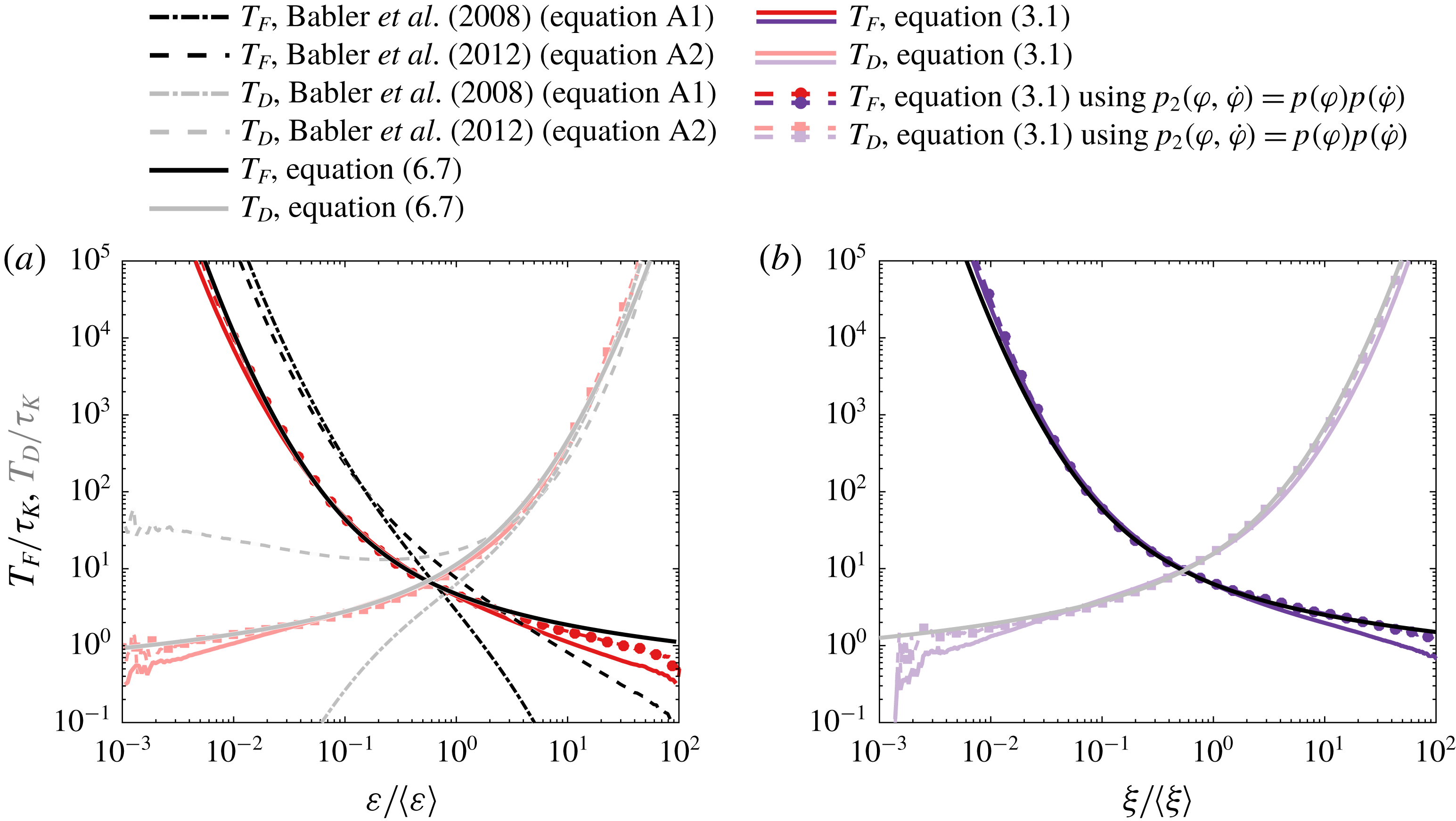
The mean flying and diving times obtained using our model (6.7) more accurately match those obtained from DNS (figure 11
a). Note however that our model logically does not capture the existing asymmetry between
 $T_{F}$
and
 $T_{D}$
since it uses a symmetrical stochastic model, and results at extreme thresholds are impacted by the fact that bursts and holes cannot be accurately modelled by log-normal statistics (figures 1 and 14). Interestingly, results of the DNS when considering uncorrelated
 $\unicode[STIX]{x1D711}$
and
 $\dot{\unicode[STIX]{x1D711}}$
in the Rice theorem were well recovered by our theoretical results of mean diving times during holes and partially captured for flying times during bursts. Hence, a better characterisation of the link between
 $\unicode[STIX]{x1D700}$
and its temporal variation during bursts and holes would lead to better predictions.
Results of mean residence times from the DNS were recovered by our model with a non-unity coefficient
 $C_{T\unicode[STIX]{x1D700}}$
of
 $1.3$
, and ratios
 $T_{F|D}/\unicode[STIX]{x03C0}(\unicode[STIX]{x1D70E}_{\ln \unicode[STIX]{x1D700}}/\unicode[STIX]{x1D70E}_{\dot{\ln \unicode[STIX]{x1D700}}})$
and
 $\unicode[STIX]{x1D70F}_{L,\unicode[STIX]{x1D712}}/\unicode[STIX]{x1D70F}_{L,\ln \unicode[STIX]{x1D700}}$
of
 $1.1$
and
 $1.2$
, respectively, hence highlighting the known departure from Gaussianity of
 $\ln \unicode[STIX]{x1D700}$
(figure 14
a) and its time derivative (figure 14
b). Results of mean times obtained from the control simulation at
 $Re_{\unicode[STIX]{x1D706}}=90$
were also recovered with our model, using
 $C_{T\unicode[STIX]{x1D700}}=1.4$
with
 $T_{F|D}/\unicode[STIX]{x03C0}(\unicode[STIX]{x1D70E}_{\ln \unicode[STIX]{x1D700}}/\unicode[STIX]{x1D70E}_{\dot{\ln \unicode[STIX]{x1D700}}})\approx 1.1$
and
 $\unicode[STIX]{x1D70F}_{L,\unicode[STIX]{x1D712}}/\unicode[STIX]{x1D70F}_{L,\ln \unicode[STIX]{x1D700}}\approx 1.3$
(see appendix D). The fact of non-unity and Reynolds number dependency of
 $C_{T\unicode[STIX]{x1D700}}$
confirms that a Gaussian-distribution-based model is not sufficient to capture Lagrangian intermittency (Chevillard et al.
Reference Chevillard, Castaing, Arneodo, Lévêque, Pinton and Roux2012).
Interestingly, although pseudo-dissipation is known to have better Gaussianity than dissipation (Yeung & Pope Reference Yeung and Pope1989; Yeung et al.
Reference Yeung, Pope, Lamorgese and Donzis2006a
), results of our model fitted the Lagrangian statistics from DNS using
 $C_{T\unicode[STIX]{x1D709}}=1.7$
, hence highlighting the impact of the non-Gaussianity of
 $\unicode[STIX]{x1D709}$
. Ratios
 $T_{F|D}/\unicode[STIX]{x03C0}(\unicode[STIX]{x1D70E}_{\ln \unicode[STIX]{x1D709}}/\unicode[STIX]{x1D70E}_{\dot{\ln \unicode[STIX]{x1D709}}})\approx 1.1$
and
 $\unicode[STIX]{x1D70F}_{L,\unicode[STIX]{x1D712}}/\unicode[STIX]{x1D70F}_{L,\ln \unicode[STIX]{x1D709}}\approx 1.5$
show that the discrepancy of our model essentially comes from the non-Gaussianity of
 $\dot{\ln \unicode[STIX]{x1D709}}$
. Moreover, our model does not capture accurately the flying and diving temporal statistics at extreme thresholds of
 $\unicode[STIX]{x1D709}$
. Considering uncorrelated
 $\unicode[STIX]{x1D709}$
and
 $\dot{\unicode[STIX]{x1D709}}$
in the Rice theorem entirely removes this departure of the DNS results from our model. Thus, the Lagrangian intermittency of
 $\unicode[STIX]{x1D709}$
can be described by the link between pseudo-dissipation and its temporal variation during bursts and holes. Since
 $\unicode[STIX]{x1D700}$
and
 $\unicode[STIX]{x1D709}$
only differ by the Reynolds stress tensor, one can conclude that the Lagrangian intermittency of
 $\unicode[STIX]{x1D700}$
during bursts and holes is characterised both by the correlation between
 $\unicode[STIX]{x1D700}$
and
 $\dot{\unicode[STIX]{x1D700}}$
and the Reynolds stress, the latter being negligible during holes.
6.1.3 Results for
$\unicode[STIX]{x1D711}=a$
,
$\unicode[STIX]{x1D714}$
and
$u$


Results of our model (6.7) for acceleration are less accurate with substantial discrepancies in the temporal statistics during holes and also deviation at very large thresholds during bursts (figure 12
a). This was expected as acceleration is normally modelled by a more complex stochastic process (Lamorgese et al.
Reference Lamorgese, Pope, Yeung and Sawford2007). Note that the deviation during bursts might again be simply due to numerical discrepancies (van Hinsberg et al.
Reference van Hinsberg, ten Thije Boonkkamp, Toschi and Clercx2013). Here too, a main portion of the deviation can be explained by the correlation between the magnitude of the acceleration and its variation rate, however, contrarily to dissipation, it is the events of holes which cannot be explained only by such correlation and during which other underlying physics appear to control the Lagrangian intermittency of acceleration. Results from DNS were fitted using
 $C_{Ta}=0.9$
, a value close to unity, however, ratios
 $T_{F|D}/\unicode[STIX]{x03C0}(\unicode[STIX]{x1D70E}_{\ln \unicode[STIX]{x1D700}}/\unicode[STIX]{x1D70E}_{\dot{\ln \unicode[STIX]{x1D700}}})\approx 1.4$
and
 $\unicode[STIX]{x1D70F}_{L,\unicode[STIX]{x1D712}}/\unicode[STIX]{x1D70F}_{L,\ln \unicode[STIX]{x1D700}}\approx 0.7$
show large deviations from Gaussianity of both
 $\ln a$
and
 $\dot{\ln a}$
but that compensate each other.
Instead, results on mean statistics of enstrophy are similar to those of dissipation with deviation of our model from our numerical results being explained by the correlation between
 $\unicode[STIX]{x1D714}$
and
 $\dot{\unicode[STIX]{x1D714}}$
entirely during holes and partially during bursts, highlighting here too the effects of other driving forces on enstrophy. Theoretical results were fitted using
 $C_{T\unicode[STIX]{x1D714}}=1.8$
with ratios
 $T_{F|D}/\unicode[STIX]{x03C0}\unicode[STIX]{x1D70E}_{\ln \unicode[STIX]{x1D700}}/\unicode[STIX]{x1D70E}_{\dot{\ln \unicode[STIX]{x1D700}}}\approx 1.2$
and
 $\unicode[STIX]{x1D70F}_{L,\unicode[STIX]{x1D712}}/\unicode[STIX]{x1D70F}_{L,\ln \unicode[STIX]{x1D700}}\approx 1.5$
, therefore showing a large deviation from Gaussianity of
 $\dot{\ln \unicode[STIX]{x1D714}}$
.
Normalised mean flying and diving residence times,
 $T_{F}/\unicode[STIX]{x1D70F}_{K}$
and
 $T_{D}/\unicode[STIX]{x1D70F}_{K}$
, with respect to (a)
 $a_{t}/\langle a\rangle$
, (b)
 $\unicode[STIX]{x1D714}_{t}/\langle \unicode[STIX]{x1D714}\rangle$
and (c)
 $u_{t}/\langle u\rangle$
derived from the Rice theorem with DNS data and from our model (6.7) (see inset legends). While the mean time statistics of enstrophy is well recovered by (6.7), especially when not considering the correlation between
 $\unicode[STIX]{x1D714}$
and
 $\dot{\unicode[STIX]{x1D714}}$
in the Rice theorem, it is less accurate in the case of acceleration. Finally, results of our model show that Lagrangian intermittency of velocity i.e. the mean time statistics during bursts and holes could be theoretically recovered should one model the correlation between
 $u$
and
 $\dot{u}$
.

Finally, it is noteworthy that, when applied to the Lagrangian velocity, our model fits numerical results using
 $C_{Tu}=2.5$
with ratios
 $T_{F|D}/\unicode[STIX]{x03C0}(\unicode[STIX]{x1D70E}_{\ln \unicode[STIX]{x1D700}}/\unicode[STIX]{x1D70E}_{\dot{\ln \unicode[STIX]{x1D700}}})\approx 1.3$
and
 $\unicode[STIX]{x1D70F}_{L,\unicode[STIX]{x1D712}}/\unicode[STIX]{x1D70F}_{L,\ln \unicode[STIX]{x1D700}}\approx 1.9$
. Thus, even though the Lagrangian velocity is known to be almost Gaussian, such large values of
 $C_{Tu}$
and corresponding ratios highlight the strong impact of the known deviation from Gaussianity of the Lagrangian variation rate of velocity (Chevillard et al.
Reference Chevillard, Castaing, Arneodo, Lévêque, Pinton and Roux2012). Surprisingly, even though our results are inferred from HIT, previous results of
 $C_{Tu}$
obtained for the Eulerian velocity in turbulent boundary layers were closer to unity (
 $1.1\pm 10\,\%$
, see Sreenivasan et al.
Reference Sreenivasan, Prabhu and Narasimha1983). Further study will be necessary to compare the Lagrangian and Eulerian statistics as well as assess the effect of the anisotropy introduced by the boundary. Our model could entirely recover the mean time statistics of the Lagrangian velocity during holes and bursts when considering uncorrelated
 $u$
and
 $\dot{u}$
, showing that the Lagrangian intermittency of velocity could be recovered with a theoretical modelling of the correlation between the velocity and its variation rate.
Thus, our model represents an overall accurate first approximation of the Lagrangian time scales of turbulence quantities in HIT. Interestingly, equations (6.7) and (6.8) state that the mean temporal statistics of turbulence quantities can be approximated knowing only their variance and those of their variation rates. In terms of time scales, this means that the mean temporal statistics of turbulent quantities can be approximated from their decorrelation time scales along with the Kolmogorov time scale. This defines
 $[\unicode[STIX]{x1D70F}_{K}-{\mathcal{T}}_{\ln \unicode[STIX]{x1D712}}]$
(with
 ${\mathcal{T}}_{\ln \unicode[STIX]{x1D712}}\approx 12\unicode[STIX]{x1D70F}_{K}$
at
 $Re_{\unicode[STIX]{x1D706}}=240$
) as the core range of time scales in turbulence.
(a,b) Profiles of mean flying (pure colours) and diving (lighter colours) times and LPDFs at
 $\unicode[STIX]{x1D700}_{t}^{s}$
derived from our DNS at
 $Re_{\unicode[STIX]{x1D706}}=240$
and Lagrangian stochastic models of Pope & Chen (Reference Pope and Chen1990), Chevillard & Meneveau (Reference Chevillard and Meneveau2006) and Lamorgese et al. (Reference Lamorgese, Pope, Yeung and Sawford2007) presented in appendix C. (b,c) Same as in (a,b) but for acceleration using data from our DNS and from the model of Lamorgese et al. (Reference Lamorgese, Pope, Yeung and Sawford2007).

6.2 Flying and diving time statistics from current Lagrangian stochastic models
Here, we assess the accuracy of current Lagrangian stochastic models in predicting the mean residence flying and diving times as well as the corresponding LPDFs in HIT. Lagrangian stochastic models have received particular interest these past decades as they represent an efficient way to compute the temporal variation of turbulence quantities. Models either focus on a specific turbulence quantity, whether velocity (Sawford Reference Sawford1991), dissipation (Pope & Chen Reference Pope and Chen1990; Lamorgese et al. Reference Lamorgese, Pope, Yeung and Sawford2007) or acceleration (Sawford Reference Sawford1991; Lamorgese et al. Reference Lamorgese, Pope, Yeung and Sawford2007), or on velocity gradients (Girimaji & Pope Reference Girimaji and Pope1990; Chevillard & Meneveau Reference Chevillard and Meneveau2006; Meneveau Reference Meneveau2011) from which can be inferred various quantities. We consider two Lagrangian stochastic models for dissipation (the models of Pope & Chen (Reference Pope and Chen1990), Chevillard & Meneveau (Reference Chevillard and Meneveau2006) and Lamorgese et al. (Reference Lamorgese, Pope, Yeung and Sawford2007)) and one for acceleration (the model of Lamorgese et al. (Reference Lamorgese, Pope, Yeung and Sawford2007)). Details on the models as well as the values of the various parameters taken for comparison with results of our DNS are given in appendix C.
Figure 13(a) shows the profiles of mean flying and diving times obtained from time series of dissipation computed with the model of Pope & Chen (Reference Pope and Chen1990), Lamorgese et al. (Reference Lamorgese, Pope, Yeung and Sawford2007), (C 3), and of Chevillard & Meneveau (Reference Chevillard and Meneveau2006), (C 6). Since all models are based on a stochastic process (i.e. the Wiener process) which, as previously explained, introduces unphysical fluctuations on scales smaller than
 $\unicode[STIX]{x1D70F}_{K}$
, the same filtering function (2.2) with
 $T_{A}=\unicode[STIX]{x1D70F}_{K}/3$
was applied to all computed time series. The model of Pope & Chen (Reference Pope and Chen1990), Lamorgese et al. (Reference Lamorgese, Pope, Yeung and Sawford2007) globally reproduces profiles of mean flying and diving times found using our DNS and captures the correct
 $\unicode[STIX]{x1D700}_{t}^{s}$
, although the corresponding mean time
 $T_{F|D}$
is slightly slower by a factor
 $1.5$
which can be explained both by the Gaussian approximation (as in our theoretical derivation) and the empirical approximations of
 $\unicode[STIX]{x1D70E}_{\ln \unicode[STIX]{x1D700}}$
and
 $T_{\ln \unicode[STIX]{x1D700}}$
(C 4) and (C 5). On the contrary, results from the model of Chevillard & Meneveau (Reference Chevillard and Meneveau2006) are not as accurate. While the statistics of mean flying times are recovered, although the model does not reach the large values obtained with DNS, with a maximum of
 $10\langle \unicode[STIX]{x1D700}\rangle$
, mean flying times are critically different than those obtained from DNS. The existing asymmetry between mean flying and diving statistics is much more accentuated than for DNS. Finally,
 $\unicode[STIX]{x1D711}_{t}^{s}$
is not recovered, however, the corresponding mean time
 $T_{F|D}$
is about the same value as that obtained with the model of Pope & Chen (Reference Pope and Chen1990), Lamorgese et al. (Reference Lamorgese, Pope, Yeung and Sawford2007).
Figure 13(b) shows the flying and diving LPDFs obtained from both models at
 $\unicode[STIX]{x1D700}_{t}^{s}$
. Both models fail to capture the distributions obtained from DNS, especially the peak at
 $\unicode[STIX]{x1D70F}_{\unicode[STIX]{x1D706}}$
. Interestingly, both models produce the same diving LPDFs. The flying LPDFs produced by the symmetrical model of Pope & Chen (Reference Pope and Chen1990), Lamorgese et al. (Reference Lamorgese, Pope, Yeung and Sawford2007) are by definition equal to the diving LPDFs. Instead, the model of Chevillard & Meneveau (Reference Chevillard and Meneveau2006) creates a slight asymmetry between flying and diving statistics but it is not consistent with that of DNS. Finally, the predominance of short flights and dives shows that the LPDFs are mainly governed by the Wiener process at numerical time step
 $\unicode[STIX]{x0394}t$
which has been filtered at
 $\unicode[STIX]{x1D70F}_{K}$
. This explains why the mean residence time
 $T_{F|D}$
at
 $\unicode[STIX]{x1D711}_{t}^{s}$
could not be recovered and is equivalent for both models since the same
 $\unicode[STIX]{x0394}t$
and filtering were used.
Figure 13(a) shows the profiles of mean flying and diving times obtained from time series of acceleration computed with the model of Lamorgese et al. (Reference Lamorgese, Pope, Yeung and Sawford2007), equation (C 9). Results are not conclusive. While flying times somewhat follow the same trend as that from DNS, mean diving times are not accurate. The magnitude
 $a_{t}^{s}$
is captured but not its corresponding residence time. This is explained here too by the predominance of small-scale fluctuations in the signals which induce peaks of the LPDFs at
 $a_{t}^{s}$
corresponding to the filtering time scale instead of that obtained from DNS (figure 13
b).
7 Discussion
We have investigated the time scales of fluctuations of three turbulence quantities, namely, the dissipation
 $\unicode[STIX]{x1D700}$
, acceleration
 $a$
and enstrophy
 $\unicode[STIX]{x1D714}$
, and their links to the flow characteristics in homogeneous isotropic turbulence by means of flying and diving Lagrangian probability density functions and flying and diving joint distributions of velocity invariants. Results are summarised and discussed below.
7.1 Statistics of bursts and holes and associated flow characteristics
We have found that for all quantities
 $\unicode[STIX]{x1D711}=\unicode[STIX]{x1D700}$
,
 $a$
or
 $\unicode[STIX]{x1D714}$
, profiles of mean flying and diving times,
 $T_{F}$
and
 $T_{D}$
, with respect to a threshold
 $\unicode[STIX]{x1D711}_{t}$
are globally symmetric about the axis
 $\unicode[STIX]{x1D711}_{t}^{s}=\langle \unicode[STIX]{x1D711}\rangle \text{e}^{-\unicode[STIX]{x1D70E}_{\ln \unicode[STIX]{x1D711}}^{2}/2}$
(figure 4). This symmetry is witness to the presence of holes, in contrast to bursts, during which the values of turbulence quantities can fall by several orders of magnitudes (figure 1). On the contrary, the existing slight asymmetry between the mean statistics of holes and bursts highlights the influence of Lagrangian intermittency.
We show that Lagrangian holes are relatively smooth and short events correlated only over a few
 $\unicode[STIX]{x1D70F}_{K}$
(figures 1, 5 and 6) and mostly correspond to periods of travel in regions in a quiescent state between turbulent flow structures (figure 8). Similar results have been found using the Eulerian dataset of our control simulation at
 $Re_{\unicode[STIX]{x1D706}}=90$
, hence suggesting a contradiction with previous studies which suggested that holes were linked to highly enstrophic filamentary vortex-like structures (She & Leveque Reference She and Leveque1994; Gledzer et al.
Reference Gledzer, Villermaux, Kahalerras and Gagne1996).
On the contrary, bursts occur over periods of time scaling with the global decorrelation time scale
 ${\mathcal{T}}_{\ln \unicode[STIX]{x1D711}}$
(figures 5 and 6) and correspond to travel inside turbulent flow structures (figures 7 and 8). Thus,
 ${\mathcal{T}}_{\ln \unicode[STIX]{x1D700}}$
does not emerge from a continuous loss of information of the flow history but, rather, from the specific correlated events of bursts. In passing, we add that, as mentioned in the introduction, previous studies have shown the existence of an anomalous Lagrangian statistics at dissipative scales which emerges from local fluctuations of the viscous scale along Lagrangian trajectories (Arneodo et al.
Reference Arneodo2008; Benzi et al.
Reference Benzi, Biferale, Fisher, Lamb and Toschi2010; Yu & Meneveau Reference Yu and Meneveau2010), and speculate that this anomalous statistics is one of the greatest obstacles to overcome for the understanding of Lagrangian intermittency (Sawford Reference Sawford2001; Yakhot & Sreenivasan Reference Yakhot and Sreenivasan2005; Zybin et al.
Reference Zybin, Sirota, Ilyin and Gurevich2008; Benzi et al.
Reference Benzi, Biferale, Fisher, Lamb and Toschi2010). This anomalous statistics has been found to occur for times up to approximately
 $10{-}20\unicode[STIX]{x1D70F}_{K}$
(Arneodo et al.
Reference Arneodo2008) which is consistent with
 ${\mathcal{T}}_{\ln \unicode[STIX]{x1D711}}$
(here approximately
 $11.5\unicode[STIX]{x1D70F}_{K}$
for
 $Re_{\unicode[STIX]{x1D706}}=240$
). Hence, the statistics obtained for larger time scales would then be the result of considering several periods of bursts and inter-bursts (included holes). Rather than being anomalous, the detected range of statistics in previous studies therefore represents the core range of Lagrangian intermittency.
Finally, for all three turbulent quantities, the flying and diving joint distributions of the invariants
 $Q_{S}$
and
 $R_{S}$
, describing the local Eulerian flow shear configuration, are self-similar. During travel, regardless of whether they are in a burst or hole, particles mostly undergo (in a statistical sense) continuous fluctuations in the level of strain which mainly characterise the passage from 2-D flow features to bi-axial stretching configurations (figure 8). It is of note that we could detect the same self-similar path using Eulerian statistics (
 $Re_{\unicode[STIX]{x1D706}}=90$
), hence showing that this existing path during holes and bursts does not depend on the referential. Such self-similar behaviour raises the question as to what property of turbulence sets the level of shear that will reach the fluid particle when leaving the 2-D configuration. It was suggested that Lagrangian intermittency of velocity, although not self-similar, emerged from a self-similar mechanism controlled by acceleration and not dissipation (Wilczek et al.
Reference Wilczek, Xu, Ouellette, Friedrich and Bodenschatz2013). Besides, it was also previously suggested that local acceleration and dissipation were statistically dependent (Lamorgese et al.
Reference Lamorgese, Pope, Yeung and Sawford2007; Liberzon et al.
Reference Liberzon, Lüthi, Holzner, Ott, Berg and Mann2012). The fact that the self-similar path always goes across a 2-D configuration at small dissipation tends to suggest that dissipation may not be the controlling mechanism. Thus, we speculate that bi-axial configurations represent the straining structures that maximise dissipation of the available local energy and that this local level of dissipation depends on the magnitude of the acceleration. Further investigation on how these turbulent quantities evolve in 2-D configurations could bring more elements of an answer.
7.2 Characteristic time scales of turbulent fluctuations
Although mean flying and diving times are equal at
 $\unicode[STIX]{x1D711}_{t}^{s}$
, the corresponding flying and diving LPDFs are not similar, showing that the dynamics ruling flights differs from that ruling dives (figures 5 and 6). For dissipation, this asymmetry is induced by Lagrangian fluctuations of the Reynolds stress which are greater during flights (figure 5). For
 $\unicode[STIX]{x1D700}$
and
 $a$
, our results show that their most probable time of flight above
 $\unicode[STIX]{x1D711}_{t}^{s}$
is approximately the Eulerian Taylor time scale
 $\unicode[STIX]{x1D70F}_{\unicode[STIX]{x1D706}}=\langle (\unicode[STIX]{x2202}u/\unicode[STIX]{x2202}x)^{2}\rangle ^{-1/2}$
while it is twice larger for
 $\unicode[STIX]{x1D714}$
. The time scale associated with the peak of the flying LPDF for
 $a$
and
 $\unicode[STIX]{x1D714}$
is however slightly Reynolds number dependent (figures 6 and 16).
Since the LPDFs are not scale specific, a physical interpretation of the dependency between
 $\unicode[STIX]{x1D70F}_{\unicode[STIX]{x1D706}}$
and flying times at
 $\unicode[STIX]{x1D700}_{t}^{s}$
is difficult. Namely, at a given threshold
 $\unicode[STIX]{x1D711}_{t}$
and residence time
 $\unicode[STIX]{x1D70F}$
, the density of the flying or diving LPDFs can represent either one specific phenomenon whose characteristic time scale is
 $\unicode[STIX]{x1D70F}$
or another phenomenon of larger characteristic time scale which mainly occurs with a smaller or larger magnitude (i.e.
 $\unicode[STIX]{x1D700}_{t}$
captures the bottom or top of the fluctuations), hence mixing different scales of the inertial cascade. Hence, our results show too that
 $\unicode[STIX]{x1D70F}_{\unicode[STIX]{x1D706}}$
is not a physical time scale per se, but, instead, a time scale characterising the entire inertial cascade rather than just the smallest eddies present in the flow (Tennekes & Lumley Reference Tennekes and Lumley1972; Pope Reference Pope2000).
Thus, when considering shear or acceleration,
 $\unicode[STIX]{x1D70F}_{\unicode[STIX]{x1D706}}$
(or
 $2\unicode[STIX]{x1D70F}_{\unicode[STIX]{x1D706}}$
for enstrophy) represents a more accurate characteristic time scale of interaction between particles and turbulence than the Kolmogorov time scale. While theoretically convenient, the Kolmogorov scale is just a mean approximation of the smallest scale in turbulence, and therefore does not hold any information on the local ongoing physics that particles undergo in turbulence. In the context of HIT, there exists a clear theoretical relationship between
 $\unicode[STIX]{x1D70F}_{K}$
and
 $\unicode[STIX]{x1D70F}_{\unicode[STIX]{x1D706}}=\sqrt{15}\unicode[STIX]{x1D70F}_{K}$
, however, this is not as straightforward for anisotropic flows, and differences between
 $\unicode[STIX]{x1D70F}_{\unicode[STIX]{x1D706}}$
and
 $\unicode[STIX]{x1D70F}_{K}$
can be larger (Arad et al.
Reference Arad, Dhruva, Kurien, Lvov, Procaccia and Sreenivasan1998). Further studies could be conducted to assess whether
 $\unicode[STIX]{x1D70F}_{\unicode[STIX]{x1D706}}$
remains a characteristic time scale for anisotropic flows.
Although our results suggests that
 $\unicode[STIX]{x1D70F}_{\unicode[STIX]{x1D706}}$
is indeed not physical, questions still remain. Why does the Eulerian Taylor time scale emerge as a characteristic time scale for Lagrangian statistics? Even if not attached to a specific physical scale, does it reflect a specific relationship between the Lagrangian and Eulerian frameworks other than the
 $\unicode[STIX]{x1D6FF}_{\unicode[STIX]{x1D70F}}v\sim \unicode[STIX]{x1D6FF}_{x}u$
hypothesis commonly considered in models of Lagrangian statistics (Biferale et al.
Reference Biferale, Boffetta, Celani, Devenish, Lanotte and Toschi2004)? Looking at flying and diving Eulerian PDFs of dissipation computed from the small Reynolds number DNS, one could see that the EPDFs had the same peak as the diving LPDFs at approximately
 $2\unicode[STIX]{x1D70F}_{K}$
instead of
 $\unicode[STIX]{x1D70F}_{\unicode[STIX]{x1D706}}$
for the flying LPDFs (figure 16
d), hence raising the interesting point that Lagrangian intermittency tends to be slower than Eulerian intermittency with a stronger asymmetry between flights and dives. However, such a result needs to be confirmed at a higher level of turbulence. Understanding why such a difference exists could bring more information about
 $\unicode[STIX]{x1D70F}_{\unicode[STIX]{x1D706}}$
.
7.3 Interpretation of the theoretical predictions
We derived an analytical approximation of
 $T_{F}$
and
 $T_{D}$
(equation (6.7)) which accurately captures variations of the mean times (figure 4) and significantly improves previous predictions (Babler et al.
Reference Babler, Morbidelli and Baldiga2008, Reference Babler, Biferale and Lanotte2012) (figure 11). Our derivation recovers (3.3) (Rice Reference Rice1945; Liepmann Reference Liepmann1949; Ylvisaker Reference Ylvisaker1965) linking the mean residence time at
 $\unicode[STIX]{x1D711}_{t}^{s}$
and the Taylor time scale for a Gaussian process and shows that the mean times of turbulent fluctuations can be predicted from the Kolmogorov mean viscous time scale
 $\unicode[STIX]{x1D70F}_{K}$
and the decorrelation time scale of the quantities’ orders of magnitude
 ${\mathcal{T}}_{\ln \unicode[STIX]{x1D711}}$
(equations (6.7) and (6.8)).
Although our predictions globally capture the trends of flying and diving mean times, discrepancies appear at extreme thresholds. The departure of the model from DNS is witness to Lagrangian intermittency during bursts and holes. For pseudo-dissipation and enstrophy, this departure could be entirely explained by the non-zero correlation between these quantities’ magnitudes and variation rates. Instead, departure of mean times of dissipation at extreme thresholds was explained both by the correlation between
 $\unicode[STIX]{x1D700}$
and
 $\dot{\unicode[STIX]{x1D700}}$
and the Reynolds stress. The correlation between
 $a$
and
 ${\dot{a}}$
could not either entirely explain Lagrangian intermittency of acceleration, showing the existence of another control mechanism on acceleration, which could be, as previously suggested, dissipation (Lamorgese et al.
Reference Lamorgese, Pope, Yeung and Sawford2007; Liberzon et al.
Reference Liberzon, Lüthi, Holzner, Ott, Berg and Mann2012).
Finally, results of flying and diving LPDFs obtained from our DNS dataset were compared to datasets of time series computed using two different Lagrangian stochastic models of dissipation (Pope & Chen Reference Pope and Chen1990; Chevillard & Meneveau Reference Chevillard and Meneveau2006) and one model for acceleration (Lamorgese et al.
Reference Lamorgese, Pope, Yeung and Sawford2007). The models could not reproduce accurately the flying and diving LPDFs obtained by DNS (figure 6). We show that these discrepancies can be partially explained by the modelling of small-scale turbulence as a random Wiener process with no specific physical scale. Using a Wiener process was supported by the fact that the viscous scale tends to 0 at infinite Reynolds number (Sawford Reference Sawford1991), however, such a hypothesis consequently removed all self-similar properties of Lagrangian statistics such as the peak of the flying LPDFs of dissipation at
 $\unicode[STIX]{x1D700}_{t}^{s}$
. Another discrepancy is that considering only one decorrelation time scale neglects the existing detected asymmetry in Lagrangian intermittency during bursts and holes which generates holes longer that in DNS by almost an order of magnitude. In the context of turbulent mixing and dispersal, where numerical predictions still need improvement (Sawford Reference Sawford2001; Toschi & Bodenschatz Reference Toschi and Bodenschatz2009), the temporal statistics we deliver in this study along with the enunciated properties of Lagrangian intermittency could help in improving Lagrangian models, although non-tested more recent existing models (Johnson & Meneveau Reference Johnson and Meneveau2017, Reference Johnson and Meneveau2018; Pereira, Moriconi & Chevillard Reference Pereira, Moriconi and Chevillard2018) may already be more accurate.
Acknowledgements
R.W. warmly thanks R. Caballero and M. Bourgoin for insightful discussions and as well as M. Babler for his help on his models. R.W. also warmly thanks an anonymous referee for pointing out to us the studies on zero-crossing theory and, more generally, the anonymous referees for their very insightful comments.
Appendix A. Statistics of
$\unicode[STIX]{x1D700}$
,
$\unicode[STIX]{x1D714}$
and
$a$


Figure 14 shows the statistics of dissipation, enstrophy and acceleration and their variations rates.
Distributions (a) in linear scale and (b) in log scale of
 $\unicode[STIX]{x1D700}$
,
 $a$
and
 $\unicode[STIX]{x1D714}$
and log-normal approximations (dashed) with
 $\unicode[STIX]{x03BC}_{\ln \unicode[STIX]{x1D700}}=-0.56$
and
 $\unicode[STIX]{x1D70E}_{\ln \unicode[STIX]{x1D700}}=1.1$
,
 $\unicode[STIX]{x03BC}_{\ln a}=2.94$
and
 $\unicode[STIX]{x1D70E}_{\ln a}=0.77$
and
 $\unicode[STIX]{x03BC}_{\ln \unicode[STIX]{x1D714}}=-0.85$
and
 $\unicode[STIX]{x1D70E}_{\ln \unicode[STIX]{x1D714}}=1.41$
. While the linear scale shows that turbulence properties can be approximated by a log-normal density profile in order to compute mean statistics, the log-scale exhibits the clear departure at extreme values which accounts for a more complex dynamics arising from bursts and holes.

Appendix B. Flow geometries: theoretical background
In fluid flows, a fluid parcel, located at an arbitrary point
 $\boldsymbol{x}_{0}$
, and moving at a velocity
 $\boldsymbol{u}(\boldsymbol{x},t)$
, follows the first-order relation
 $$\begin{eqnarray}\boldsymbol{u}(\boldsymbol{x},t)=\boldsymbol{u}(\boldsymbol{x}_{0},t)+\unicode[STIX]{x1D63C}(\boldsymbol{x}_{0},t)(\boldsymbol{x}-\boldsymbol{x}_{0}),\end{eqnarray}$$
where
 $\unicode[STIX]{x1D608}_{ij}=\unicode[STIX]{x2202}u_{i}/\unicode[STIX]{x2202}x_{j}$
is the velocity gradient tensor and describes the local velocity field surrounding the parcel;
 $\unicode[STIX]{x1D63C}$
contains the information about the first-order near-future directions and curvatures taken by the particle. Hence, the velocity gradient tensor allows us to describe the flow structures surrounding the particle on a small time scale. In turbulence, the linear expansion holds for a time of the order of the local viscous scale
 $\unicode[STIX]{x1D70F}_{K}(\unicode[STIX]{x1D700})=(\unicode[STIX]{x1D708}/\unicode[STIX]{x1D700}^{3})^{1/4}$
(Meneveau Reference Meneveau2011).
B.1 The velocity invariants
The eigenvectors and eigenvalues of
 $\unicode[STIX]{x1D608}_{ij}$
define the principal directions and magnitudes of influence of velocity gradients, respectively. Each eigenvalue of
 $\unicode[STIX]{x1D608}_{ij}$
,
 $\unicode[STIX]{x1D706}_{i}$
, satisfies the following characteristic equation
 $$\begin{eqnarray}\unicode[STIX]{x1D706}_{i}^{3}+P_{A}\unicode[STIX]{x1D706}_{i}^{2}+Q_{A}\unicode[STIX]{x1D706}_{i}+R_{A}=0,\end{eqnarray}$$
where
 $P_{A}=-\unicode[STIX]{x1D608}_{ii}$
,
 $Q_{A}=-\unicode[STIX]{x1D608}_{ij}\unicode[STIX]{x1D608}_{ji}$
and
 $R_{A}=-\unicode[STIX]{x1D608}_{ij}\unicode[STIX]{x1D608}_{jk}\unicode[STIX]{x1D608}_{ki}$
are the so-called first, second and third invariants, respectively, i.e. tensors independent of the orientation of the coordinate system and that characterise the flow structure. The velocity tensor is the sum of strain and rotation terms,
 $\unicode[STIX]{x1D608}_{ij}=\unicode[STIX]{x1D61A}_{ij}+\unicode[STIX]{x1D61E}_{ij}$
. Similarly to (B 2),
 $\unicode[STIX]{x1D61A}_{ij}$
and
 $\unicode[STIX]{x1D61E}_{ij}$
also have a characteristic equation with their corresponding invariants (
 $P_{S}$
,
 $Q_{S}=-(1/2)\unicode[STIX]{x1D61A}_{ij}\unicode[STIX]{x1D61A}_{ij}$
,
 $R_{S}=-(1/3)\unicode[STIX]{x1D61A}_{ij}\unicode[STIX]{x1D61A}_{jk}\unicode[STIX]{x1D61A}_{ki}$
) and (
 $P_{W}=0$
,
 $Q_{W}=(1/2)\unicode[STIX]{x1D61E}_{ij}\unicode[STIX]{x1D61E}_{ij}$
,
 $R_{W}=0$
), respectively. For an incompressible flow, one has
 $P_{A}=0$
and
 $P_{S}=0$
, and the invariants of
 $\unicode[STIX]{x1D608}_{ij}$
are related as:
 $$\begin{eqnarray}\displaystyle & \displaystyle Q_{A}=Q_{S}+Q_{W}; & \displaystyle\end{eqnarray}$$
 $$\begin{eqnarray}\displaystyle & \displaystyle R_{A}=R_{S}-{\textstyle \frac{1}{4}}\unicode[STIX]{x1D61E}_{ij}\unicode[STIX]{x1D61E}_{jk}\unicode[STIX]{x1D61A}_{ki}. & \displaystyle\end{eqnarray}$$
The set of five invariants (
 $Q_{S}$
,
 $R_{S}$
,
 $Q_{W}$
,
 $Q_{A}$
and
 $R_{A}$
) represents a first-order description of the flow configuration in a region wide of
 $\unicode[STIX]{x1D70F}_{K}$
. This flow configuration is characterised by the joint study of the invariants in phase spaces (
 $Q_{S}$
,
 $R_{S}$
), (
 $-Q_{S}$
,
 $Q_{W}$
) and (
 $Q_{A}$
,
 $R_{A}$
) that we now describe.
B.2 Characterisation of the local flow geometry
A brief explanation is given here about velocity invariants and their relations to flow structures in HIT. More details and analysis on the invariants in such context can also be found in Chong et al. (Reference Chong, Perry and Cantwell1990), Cantwell (Reference Cantwell1993), Perry & Chong (Reference Perry and Chong1994), Soria et al. (Reference Soria, Sondergaard, Cantwell, Chong and Perry1994), Martin et al. (Reference Martin, Ooi, Chong and Soria1998), Ooi et al. (Reference Ooi, Martin, Soria and Chong1999), Wang et al. (Reference Wang, Bergstrom, Yin and Yee2006), da Silva & Pereira (Reference da Silva and Pereira2008), Meneveau (Reference Meneveau2011).
The joint probability density function (JPDF) (
 $Q_{S}$
,
 $R_{S}$
) (figure 7
a) gives information on the local structure of the straining component of the flow. The term
 $Q_{S}$
corresponds to the straining intensity and is therefore directly linked to the dissipation rate
 $Q_{S}=-\unicode[STIX]{x1D700}/4\unicode[STIX]{x1D708}$
. The term
 $R_{S}$
influences the production of strain, where
 $R_{S}<0$
means a decrease of the production of strain (and
 $R_{S}>0$
is the reverse). It can be shown that
 $R_{S}=-\unicode[STIX]{x1D6FC}_{S}\unicode[STIX]{x1D6FD}_{S}\unicode[STIX]{x1D6FE}_{S}$
where
 $\unicode[STIX]{x1D6FC}_{S}\geqslant \unicode[STIX]{x1D6FD}_{S}\geqslant \unicode[STIX]{x1D6FE}_{S}$
are the principal strain rates (or eigenvalues) of
 $\unicode[STIX]{x1D61A}_{ij}$
. Given the condition of incompressibility, one has
 $\unicode[STIX]{x1D6FC}_{S}+\unicode[STIX]{x1D6FD}_{S}+\unicode[STIX]{x1D6FE}_{S}=0$
, and
 $R_{S}>0$
induces
 $\unicode[STIX]{x1D6FC}_{S},\unicode[STIX]{x1D6FD}_{S}>0$
and
 $\unicode[STIX]{x1D6FE}_{S}<0$
. The corresponding local flow structure has therefore two directions of strain production i.e. it is a sheet-like expending structure. On the other hand, when
 $R_{S}<0$
, one has
 $\unicode[STIX]{x1D6FC}_{S}>0$
and
 $\unicode[STIX]{x1D6FD}_{S},\unicode[STIX]{x1D6FE}_{S}<0$
, and the flow structure only has one direction of strain production i.e. it is a tube-like contracting structure. Since
 $\unicode[STIX]{x1D61A}_{ij}$
is a symmetric tensor, invariants
 $Q_{S}$
and
 $R_{S}$
of the flow can only lie below the null of the corresponding discriminant curve
 $D_{S}=\frac{27}{4}R_{S}^{2}+Q_{S}^{3}$
. As
 $R_{S}=-\unicode[STIX]{x1D6FC}_{S}\unicode[STIX]{x1D6FD}_{S}\unicode[STIX]{x1D6FE}_{S}$
and, with incompressibility,
 $\unicode[STIX]{x1D6FC}_{S}+\unicode[STIX]{x1D6FD}_{S}+\unicode[STIX]{x1D6FE}_{S}=0$
, one can infer that the curve
 $D_{S}=0$
for
 $R_{S}>0$
represents an axisymmetric expansion strain flow with geometry
 $\unicode[STIX]{x1D6FC}_{S}:\unicode[STIX]{x1D6FD}_{S}:\unicode[STIX]{x1D6FE}_{S}=1:1:-2$
whereas the curve
 $D_{S}=0$
for
 $R_{S}<0$
represents an axisymmetric contraction strain flow with geometry
 $2:-1:-1$
. Various other straining structures exist in between those two former configurations (Ashurst et al.
Reference Ashurst, Kerstein, Kerr and Gibson1987; Soria et al.
Reference Soria, Sondergaard, Cantwell, Chong and Perry1994; Blackburn, Mansour & Cantwell Reference Blackburn, Mansour and Cantwell1996). It has been shown (Lund & Rogers Reference Lund and Rogers1994) that the measure
 $$\begin{eqnarray}s^{\star }={\displaystyle \frac{-3\sqrt{6}\unicode[STIX]{x1D6FC}_{S}\unicode[STIX]{x1D6FD}_{S}\unicode[STIX]{x1D6FE}_{S}}{\unicode[STIX]{x1D6FC}_{S}^{2}+\unicode[STIX]{x1D6FD}_{S}^{2}+\unicode[STIX]{x1D6FE}_{S}^{2}}}^{3/2}\end{eqnarray}$$
accurately describes the local straining configuration. Given that
 $Q_{S}=-1/2(\unicode[STIX]{x1D6FC}_{s}^{2}+\unicode[STIX]{x1D6FD}_{S}^{2}+\unicode[STIX]{x1D6FE}_{S}^{2})$
and
 $R_{S}=-\unicode[STIX]{x1D6FC}_{S}\unicode[STIX]{x1D6FD}_{S}\unicode[STIX]{x1D6FE}_{S}$
, and defining
 $a=\unicode[STIX]{x1D6FD}_{S}/\unicode[STIX]{x1D6FC}_{S}$
, one can derive that lines of constant
 $s^{\star }$
follow the equation (Lund & Rogers Reference Lund and Rogers1994; da Silva & Pereira Reference da Silva and Pereira2008)
 $$\begin{eqnarray}R_{S}=(-Q_{S})^{3/2}{\displaystyle \frac{a(1+a)}{(1+a+a^{2})^{3/2}}}.\end{eqnarray}$$
The ratio
 $a$
defines a given flow geometry (
 $\unicode[STIX]{x1D6FE}_{S}$
is inferred from the condition of incompressibility). Figure 7(a) shows lines for five different straining configurations corresponding to
 $\unicode[STIX]{x1D6FC}_{s}:\unicode[STIX]{x1D6FD}_{S}:\unicode[STIX]{x1D6FE}_{S}=1:1:-2$
(
 $a=1$
and
 $D_{S}=0$
) for an axisymmetric expanding strain,
 $2:1:-3$
(
 $a=1/2$
) and
 $3:1:-4$
(
 $a=1/3$
) for biaxial-like structures,
 $1:0:-1$
(
 $a=0$
) for 2-D flows and
 $2:-1:-1$
(
 $a=-1/2$
and
 $D_{S}=0$
) for axisymmetric contraction strain node.
The JPDF (
 $-Q_{S}$
,
 $Q_{W}$
) (figure 7
c) separates dissipative and enstrophic flow structures. Large negative values of
 $Q_{S}$
imply a straining structure whereas large values of
 $Q_{W}$
are a sign of a vortical structure. A large enstrophy with weak dissipation (
 $Q_{W}\gg -Q_{S}$
) is characteristic of solid body rotations encountered in vortex tubes, while a large dissipation with weak enstrophy (
 $Q_{W}\ll -Q_{S}$
) is characteristic of irrotational dissipative regions such as in the surrounding of the vortex tubes. Regions where enstrophy scales with dissipation (
 $Q_{W}\approx -Q_{S}$
) occur in vortex sheet structures.
Finally, the JPDF (
 $Q_{A}$
,
 $R_{A}$
) (figure 7
b) highlights in which of the four non-degenerate local flow topologies the studied parcel of fluid is, namely, either a stretching or compressive vortex or a tube-like or sheet-like straining node (Soria et al.
Reference Soria, Sondergaard, Cantwell, Chong and Perry1994; Ooi et al.
Reference Ooi, Martin, Soria and Chong1999). The discrimination between vortical and straining structures is done by looking how many complex eigenvalues exist in the system. When the discriminant of
 $\unicode[STIX]{x1D608}_{ij}$
,
 $D_{A}=\frac{27}{4}R_{A}^{2}+Q_{A}^{3}$
is negative, then only one eigenvalue of
 $\unicode[STIX]{x1D608}_{ij}$
is real, and there is a plane defined by the two complex-conjugate eigenvalues in which exists a focus point for fluid parcel trajectories. On the contrary, when
 $D_{A}<0$
, all three eigenvalues are real, and there exist three planes with trajectory solutions without focus, hence a node is present. The invariant
 $R_{A}$
discriminates between stable or unstable geometries. When
 $Q_{A}>0$
, enstrophy dominates, so
 $R_{A}\sim -\frac{1}{4}\unicode[STIX]{x1D61E}_{ij}\unicode[STIX]{x1D61E}_{jk}\unicode[STIX]{x1D61A}_{ki}$
, and since
 $D_{A}>0$
, there is a plane of rotation, hence if
 $R_{A}<0$
, the fluid faces a vortex stretching, while if
 $R_{A}>0$
it is in a vortex compression. On the contrary, when
 $Q_{A}<0$
and
 $D_{A}<0$
, dissipation dominates
 $R_{A}\sim R_{S}$
, hence,
 $R_{A}<0$
describes a tube-like structure with large strain rate, and
 $R_{A}>0$
describes a sheet-like structure with large strain rate.
B.3 Computation of the joint distributions of invariants
At the time we ran the simulations of HIT, the utilised numerical code was computing the Lagrangian using a tri-linear interpolation method. This method generates discrepancies for high-order terms such as invariants (van Hinsberg et al.
Reference van Hinsberg, ten Thije Boonkkamp, Toschi and Clercx2013), with the consequence that the theoretical limit
 $D_{S}=0$
was sometimes not fulfilled. We thus filtered out time series where this limit was violated. The effect of this filtering was visible only for distributions in the space (
 $Q_{S}$
,
 $R_{S}$
) (figure 15).
Joint distributions of (a,d)
 $-Q_{S}$
versus
 $Q_{W}$
, (b,e)
 $Q_{A}$
versus
 $R_{A}$
and (c,f)
 $R_{S}$
versus
 $Q_{S}$
when (a–c) considering all Lagrangian data and (d–f) removing Lagrangian trajectories that violated the theoretical limit
 $D_{S}=0$
. The effect of such removal is only visible in the distributions
 $R_{S}$
,
 $Q_{S}$
which accurately follow the line
 $D_{S}=0$
.

The flying (diving) joint distributions shown in figure 8 correspond to initial times of flight (dive) and times of maximum (minimum) value during flights (dives). Considering only these specific later times means that most of the Lagrangian data are discarded when computed the distributions and that distributions can be scarce. To ensure robustness, a first round of computation has been conducted on the total phase space of the invariants in order to infer the range of variations of flights and dives, then a second round was made using a highly resolved discretisation of the corresponding phase space of flights and dives. Third, the derived 2-D histograms were coarse so that continuity of the joint distributions was ensured. And finally, a 2-D Gaussian convolution with half-width the size of the coarse discretisation was applied to the distributions to filter out grid-scale noise.
Flying and diving joint distributions of dissipation and enstrophy for thresholds
 $C=1/20$
and
 $40$
and of acceleration for thresholds
 $C=1/10$
and
 $20$
could not fulfil the condition of continuity due to lack of data. The difference between a coefficient smaller and larger than
 $1$
is due to the difference in physics during holes and bursts. Since holes are smoother and shorter events than bursts, less data are accessible for the flying joint distributions during holes compared to the diving joint distributions during bursts. Moreover, the lack of data for acceleration at thresholds closer to
 $a_{t}^{s}$
than for dissipation and enstrophy is explained by a smaller variance which can be seen in the mean time profiles (figure 4).
Since time periods between which the joint distributions at different key times are derived are not large, it is assumed that results give an accurate picture of the evolution of the flow characteristics along Lagrangian bursts and holes. In the case of Lagrangian holes, dissipation is found to be systematically small regardless of which quantity one considers. Hence, the corresponding local viscous time scale is large. If one considers the threshold
 $\langle \unicode[STIX]{x1D700}\rangle /20$
(
 $C=1/10$
with
 $\unicode[STIX]{x1D700}_{t}^{s}\approx \langle \unicode[STIX]{x1D700}\rangle /2$
), one has a minimum local viscous time scale during holes of
 $\unicode[STIX]{x1D70F}_{K}(\unicode[STIX]{x1D700})=10\unicode[STIX]{x1D70F}_{K}$
, a time larger than the most probable time delay between joint distributions (similar to the most probable diving time) of maximum
 $1-2\unicode[STIX]{x1D70F}_{K}$
(figure 5), hence suggesting a continuous transition between the distributions and therefore an accurate capture of the evolution of the characteristics of the Eulerian structures along Lagrangian holes. In the case of Lagrangian bursts (in the case C=20), the local viscous scale is approximately
 $\unicode[STIX]{x1D70F}_{K}(\unicode[STIX]{x1D700})=\unicode[STIX]{x1D70F}_{K}/5$
while the time delay between the joint distributions are mostly approximately
 $0.8-1\unicode[STIX]{x1D70F}_{K}$
(figure 5), hence suggesting that potential undetected variations in the invariants space. We however believe that the difference in time remains small enough so that the detected large consistent differences or similarities between the joint distributions can be considered interesting for the study of the evolution of the characteristics of the flow structures during Lagrangian bursts.
Appendix C. Modelling of Lagrangian temporal statistics
C.1 Models of
$T_{D}(\unicode[STIX]{x1D700}_{t})$
and
$T_{F}(\unicode[STIX]{x1D700}_{t})$
from Babler et al. (Reference Babler, Morbidelli and Baldiga2008, Reference Babler, Biferale and Lanotte2012)


Two models of
 $T_{F}$
and
 $T_{D}$
have already been developed in the case of dissipation (Babler et al.
Reference Babler, Morbidelli and Baldiga2008, Reference Babler, Biferale and Lanotte2012). The first model considers that
 $p_{2}$
is governed by the variation rate of dissipation at
 $\unicode[STIX]{x1D700}_{t}$
which primarily depends on the local Kolmogorov scale at
 $\unicode[STIX]{x1D700}_{t}$
,
 $\dot{\unicode[STIX]{x1D700}}\sim \unicode[STIX]{x1D700}_{t}/\unicode[STIX]{x1D70F}_{K}(\unicode[STIX]{x1D700}_{t})$
, hence giving that the joint distribution time of dissipation and its time derivative scale with
 $p(\unicode[STIX]{x1D700}_{t},\dot{\unicode[STIX]{x1D700}})\sim 1/2p(\unicode[STIX]{x1D700}_{t})\unicode[STIX]{x1D6FF}(|\dot{\unicode[STIX]{x1D700}}|-\unicode[STIX]{x1D700}_{t}/\unicode[STIX]{x1D70F}_{K}(\unicode[STIX]{x1D700}_{t}))$
. Injecting this scaling into (3.1) for
 $\unicode[STIX]{x1D711}=\unicode[STIX]{x1D700}$
gives
 $$\begin{eqnarray}T_{F}^{I}\sim \frac{\displaystyle \int _{\unicode[STIX]{x1D700}_{t}}^{\infty }\,\text{d}\unicode[STIX]{x1D700}p(\unicode[STIX]{x1D700})}{1/2\unicode[STIX]{x1D700}_{t}p(\unicode[STIX]{x1D700}_{t})/\unicode[STIX]{x1D70F}_{K}(\unicode[STIX]{x1D700}_{t})},\quad T_{D}^{I}\sim \frac{\displaystyle \int _{0}^{\unicode[STIX]{x1D700}_{t}}\,\text{d}\unicode[STIX]{x1D700}p(\unicode[STIX]{x1D700})}{1/2\unicode[STIX]{x1D700}_{t}p(\unicode[STIX]{x1D700}_{t})/\unicode[STIX]{x1D70F}_{K}(\unicode[STIX]{x1D700}_{t})}.\end{eqnarray}$$
The second model assumes that the joint distribution of dissipation and its variation rate are mainly dictated by the local Kolmogorov scale
 $p_{2}(\unicode[STIX]{x1D700},\dot{\unicode[STIX]{x1D700}})\sim p(\unicode[STIX]{x1D700})/\unicode[STIX]{x1D70F}_{K}(\unicode[STIX]{x1D700})$
and that the resulting characteristic time spent in regions above (below)
 $\unicode[STIX]{x1D700}_{t}$
is given by the variation rate in regions above (below)
 $\unicode[STIX]{x1D700}_{t}$
, hence giving
 $$\begin{eqnarray}T_{F}^{II}\sim \frac{\displaystyle \int _{\unicode[STIX]{x1D700}_{t}}^{\infty }p(\unicode[STIX]{x1D700})\,\text{d}\unicode[STIX]{x1D700}}{\displaystyle \int _{0}^{\unicode[STIX]{x1D700}_{t}}p(\unicode[STIX]{x1D700})/\unicode[STIX]{x1D70F}_{K}(\unicode[STIX]{x1D700})\,\text{d}\unicode[STIX]{x1D700}},\quad T_{D}^{II}\sim \frac{\displaystyle \int _{0}^{\unicode[STIX]{x1D700}_{t}}p(\unicode[STIX]{x1D700})\,\text{d}\unicode[STIX]{x1D700}}{\displaystyle \int _{\unicode[STIX]{x1D700}_{t}}^{\infty }p(\unicode[STIX]{x1D700})/\unicode[STIX]{x1D70F}_{K}(\unicode[STIX]{x1D700})\,\text{d}\unicode[STIX]{x1D700}}.\end{eqnarray}$$
C.2 Model of dissipation of Pope & Chen (Reference Pope and Chen1990), Lamorgese et al. (Reference Lamorgese, Pope, Yeung and Sawford2007)
The model considers that the dynamics of the order of magnitude of dissipation
 $\unicode[STIX]{x1D712}(t)=\ln (\unicode[STIX]{x1D700}/\overline{\unicode[STIX]{x1D700}})$
is modelled as an Ornstein–Uhlenbeck process:
 $$\begin{eqnarray}\text{d}\unicode[STIX]{x1D712}=-(\unicode[STIX]{x1D712}-\overline{\unicode[STIX]{x1D712}})\frac{\text{d}t}{T_{\unicode[STIX]{x1D712}}}+\left(\frac{2\unicode[STIX]{x1D70E}_{\unicode[STIX]{x1D712}}^{2}}{T_{\unicode[STIX]{x1D712}}}\right)^{1/2}\,\text{d}{\mathcal{W}},\end{eqnarray}$$
where
 $T_{\unicode[STIX]{x1D712}}=\int \langle \unicode[STIX]{x1D712}(t)\unicode[STIX]{x1D712}(t+\unicode[STIX]{x1D70F})\rangle /\langle \unicode[STIX]{x1D712}(t)^{2}\rangle \,\text{d}\unicode[STIX]{x1D70F}$
is the decorrelation time scale of
 $\unicode[STIX]{x1D712}$
,
 $\unicode[STIX]{x1D70E}_{\unicode[STIX]{x1D712}}$
is the variance of
 $\unicode[STIX]{x1D712}$
and
 ${\mathcal{W}}$
is a Wiener process whose increments are taken from a random Gaussian process with zero mean and variance
 $dt$
. Note that by construction
 $\overline{\unicode[STIX]{x1D712}}=-1/2\unicode[STIX]{x1D70E}_{\unicode[STIX]{x1D712}}^{2}$
(Pope & Chen Reference Pope and Chen1990).
Both
 $\unicode[STIX]{x1D70E}_{\unicode[STIX]{x1D712}}$
and
 $T_{\unicode[STIX]{x1D712}}$
have been determined in more recent studies empirically as a function of the Taylor-scale Reynolds number
 $Re_{\unicode[STIX]{x1D706}}$
(Yeung et al.
Reference Yeung, Pope, Lamorgese and Donzis2006a
; Lamorgese et al.
Reference Lamorgese, Pope, Yeung and Sawford2007), following
 $$\begin{eqnarray}\displaystyle & \displaystyle \unicode[STIX]{x1D70E}_{\unicode[STIX]{x1D712}}=A+\frac{3\unicode[STIX]{x03BC}}{2}\ln Re_{\unicode[STIX]{x1D706}} & \displaystyle\end{eqnarray}$$
 $$\begin{eqnarray}\displaystyle & \displaystyle T_{\unicode[STIX]{x1D712}}=T^{\infty }(0.055+3.55/Re_{\unicode[STIX]{x1D706}}^{0.7}), & \displaystyle\end{eqnarray}$$
with
 $\unicode[STIX]{x03BC}=0.25$
and
 $A=-0.863$
(Yeung et al.
Reference Yeung, Pope, Lamorgese and Donzis2006a
). The integral time scale is
 $T^{\infty }=3/2\unicode[STIX]{x1D70E}_{U}^{2}/\langle \unicode[STIX]{x1D700}\rangle$
, and can be approximated in the context of isotropic turbulence as
 $T^{\infty }=(3/20)^{1/2}Re_{\unicode[STIX]{x1D706}}\unicode[STIX]{x1D70F}_{K}$
. Results from our DNS give
 $\unicode[STIX]{x1D70E}_{\unicode[STIX]{x1D712}}=1.09$
and
 $T_{\unicode[STIX]{x1D712}}=11.98\unicode[STIX]{x1D70F}_{K}$
, both values close to those obtained with (C 5) for our Taylor-scale Reynolds number
 $Re_{\unicode[STIX]{x1D706}}=240$
. Note that an Ornstein–Uhlenbeck process generates a purely Gaussian signal. This entails that no asymmetry between the statistics of flights and dives can be produced. Thus, flying and diving statistics inferred from this model are by definition symmetric.
C.3 Model of dissipation of Chevillard & Meneveau (Reference Chevillard and Meneveau2006)
The model of Chevillard & Meneveau (Reference Chevillard and Meneveau2006) reproduces the Lagrangian time evolution of the velocity gradient tensor
 $\unicode[STIX]{x1D608}_{ij}=\unicode[STIX]{x2202}_{i}u_{j}$
. Starting from the equation of Lagrangian evolution of
 $\unicode[STIX]{x1D608}_{ij}$
derived from the incompressible Navier–Stokes equation, the authors make a series of assumptions which eventually lead to the following one-dimensional equation for the velocity gradient tensor:
 $$\begin{eqnarray}\text{d}\unicode[STIX]{x1D63C}=\left(-\unicode[STIX]{x1D63C}^{2}+{\displaystyle \frac{\text{Tr}(\unicode[STIX]{x1D63C}^{2})}{\text{Tr}(\boldsymbol{C}_{\unicode[STIX]{x1D70F}_{K}}^{-1})}}\boldsymbol{C}_{\unicode[STIX]{x1D70F}_{K}}^{-1}-{\displaystyle \frac{1}{T_{Ad}}}{\displaystyle \frac{\text{Tr}(\boldsymbol{C}_{\unicode[STIX]{x1D70F}_{K}}^{-1})}{3}}\unicode[STIX]{x1D63C}\right)\text{d}t+\text{d}\unicode[STIX]{x1D652},\end{eqnarray}$$
where
 $\boldsymbol{C}_{\unicode[STIX]{x1D70F}_{K}}=\text{e}^{\unicode[STIX]{x1D70F}_{K}\unicode[STIX]{x1D63C}}\text{e}^{\unicode[STIX]{x1D70F}_{K}\unicode[STIX]{x1D63C}^{\text{T}}}$
is an approximation of the Cauchy–Green tensor accounting for the evolution of the deformation gradients of the fluid, and
 $T_{A}$
is the Lagrangian decorrelation time scale of
 $\unicode[STIX]{x1D608}_{ij}$
, considered here as
 $T_{Ad}=\int \langle \unicode[STIX]{x1D700}(t)^{1/2}\unicode[STIX]{x1D700}(t+\unicode[STIX]{x1D70F})^{1/2}\rangle /\langle \unicode[STIX]{x1D700}(t)\rangle \,\text{d}t$
. Finally,
 $\text{d}\unicode[STIX]{x1D652}$
is a tensorial white and Gaussian noise, i.e.
 $\text{d}\unicode[STIX]{x1D61E}_{ij}=\unicode[STIX]{x1D60B}_{ijkl}\,\text{d}\unicode[STIX]{x1D609}_{kl}$
, where
 $\text{d}\unicode[STIX]{x1D609}_{ij}$
is a tensorial isotropic Wiener process with zero mean and a variance of
 $2\text{d}t$
and
 $\unicode[STIX]{x1D60B}_{ijkl}$
are the diffusion coefficients such that
 $\text{d}\unicode[STIX]{x1D652}$
is consistent with an isotropic homogeneous and traceless tensorial field. Considering that
 $\unicode[STIX]{x1D63F}$
is itself isotropic, one gets (Chevillard et al.
Reference Chevillard, Meneveau, Biferale and Toschi2008)
 $$\begin{eqnarray}\unicode[STIX]{x1D60B}_{ijkl}=a\unicode[STIX]{x1D6FF}_{ij}\unicode[STIX]{x1D6FF}_{kl}+b\unicode[STIX]{x1D6FF}_{ik}\unicode[STIX]{x1D6FF}_{jl}+c\unicode[STIX]{x1D6FF}_{il}\unicode[STIX]{x1D6FF}_{jk}\end{eqnarray}$$
with
 $$\begin{eqnarray}a={\displaystyle \frac{1}{3}}{\displaystyle \frac{3+\sqrt{15}}{\sqrt{10}+\sqrt{6}}};\quad b=-{\displaystyle \frac{\sqrt{10}+\sqrt{6}}{4}};\quad c={\displaystyle \frac{1}{\sqrt{10}+\sqrt{6}}}.\end{eqnarray}$$
The dissipation is then obtained from results of the velocity gradient invariant following
 $2\unicode[STIX]{x1D708}\unicode[STIX]{x1D61A}_{ij}\unicode[STIX]{x1D61A}_{ij}$
with
 $\unicode[STIX]{x1D61A}_{ij}=1/2(\unicode[STIX]{x1D608}_{ij}+\unicode[STIX]{x1D608}_{ji})$
.
Using our DNS dataset for
 $Re_{\unicode[STIX]{x1D706}}=240$
, we obtained
 $T_{Ad}=10.5\unicode[STIX]{x1D70F}_{K}$
.
C.4 Model of acceleration of Lamorgese et al. (Reference Lamorgese, Pope, Yeung and Sawford2007)
The model of Lamorgese et al. (Reference Lamorgese, Pope, Yeung and Sawford2007) considers that in an isotropic turbulent flow, the dynamics of the components of acceleration can be approximated as a second-order auto-regressive model, giving the stochastic differential equation:
 $$\begin{eqnarray}\text{d}a=-\unicode[STIX]{x1D6FC}_{1}\unicode[STIX]{x1D712}^{\prime }\,\text{d}t-\unicode[STIX]{x1D6FC}_{2}\int _{0}^{t}\unicode[STIX]{x1D712}^{\prime }\,\text{d}t^{\prime }\,\text{d}t+(2\unicode[STIX]{x1D6FC}_{1}\unicode[STIX]{x1D6FC}_{2}\unicode[STIX]{x1D70E}_{U}^{2})^{1/2}\,\text{d}{\mathcal{W}}.\end{eqnarray}$$
Time scales of the system are the integral time scale
 $\unicode[STIX]{x1D70F}=3/2\unicode[STIX]{x1D70E}_{U}^{2}/\unicode[STIX]{x1D700}$
, the velocity decorrelation time scale
 $T_{L}=\int _{0}^{\infty }\langle u_{i}(t)u_{i}(t+\unicode[STIX]{x1D70F})\rangle /\langle u_{i}(t)u_{i}(t)\rangle \,\text{d}\unicode[STIX]{x1D70F}$
and the acceleration time scale
 $\unicode[STIX]{x1D70F}_{a}=(\unicode[STIX]{x1D700}^{3}/\unicode[STIX]{x1D708})^{1/4}$
(Pope Reference Pope2002), giving
 $\unicode[STIX]{x1D6FC}_{1}=T_{L}/(\unicode[STIX]{x1D70F}\unicode[STIX]{x1D70F}_{a})$
and
 $\unicode[STIX]{x1D6FC}_{2}=1/(\unicode[STIX]{x1D70F}\unicode[STIX]{x1D70F}_{a})$
. Various theoretical relationships linking
 $T_{L}$
and
 $\unicode[STIX]{x1D70E}_{U}$
to the Taylor Reynolds number
 $Re_{\unicode[STIX]{x1D706}}$
have been obtained empirically (Sawford Reference Sawford1991). However, in order not to depend on any potential discrepancy in these relations at large Reynolds number (these relations have been derived with data up to
 $Re_{\unicode[STIX]{x1D706}}=90$
), the various time scales have been determined using our DNS dataset, giving:
 $$\begin{eqnarray}\unicode[STIX]{x1D70F}\approx 91.3\unicode[STIX]{x1D70F}_{K}\quad \text{and}\quad T_{L}\approx 18.8\unicode[STIX]{x1D70F}_{K},\end{eqnarray}$$
and with
 $\unicode[STIX]{x1D70F}_{a}\approx 12.6\unicode[STIX]{x1D70F}_{K}$
.
C.5 Set-up of simulations using stochastic models
We used two Lagrangian stochastic models of dissipation (Pope & Chen Reference Pope and Chen1990; Chevillard & Meneveau Reference Chevillard and Meneveau2006; Lamorgese et al.
Reference Lamorgese, Pope, Yeung and Sawford2007) and one of acceleration (Lamorgese et al.
Reference Lamorgese, Pope, Yeung and Sawford2007) to compute
 $5\times 10^{5}$
time series of time duration equal to that of our DNS, i.e.
 $T=245\unicode[STIX]{x1D70F}_{K}$
. It is important to note that since all models considered in the study use a Wiener process, we applied the filtering function (2.2) with
 $T_{A}=\unicode[STIX]{x1D70F}_{K}/3$
to the computed time series to remove the dependency on time scales below
 $\unicode[STIX]{x1D70F}_{K}$
. We then derived for each set of time series the flying and diving LPDFs and compared the results to those obtained with the DNS. Lagrangian stochastic models are described and values of the various parameters used in our DNS are given.
Appendix D. Statistics of flying and diving times at intermediate Reynolds number
To verify that our results hold true at a different level of turbulence, we simulated a HIT at smaller Taylor Reynolds number
 $Re_{\unicode[STIX]{x1D706}}=90$
and computed the flying and diving LPDFs of dissipation using
 $10^{5}$
Lagrangian trajectories.
(a) Mean flying and diving times with respect to threshold
 $\unicode[STIX]{x1D700}_{t}$
and (b) flying and diving LPDFs at corresponding
 $\unicode[STIX]{x1D711}_{t}^{s}=\unicode[STIX]{x1D700}_{t}^{s}$
,
 $\unicode[STIX]{x1D714}_{t}^{s}$
and
 $a_{t}^{s}$
computed using the Lagrangian dataset of the simulation at
 $Re_{\unicode[STIX]{x1D706}}=90$
. Results are consistent with those at
 $Re_{\unicode[STIX]{x1D706}}=245$
, specifically the Taylor scale
 $\unicode[STIX]{x1D70F}_{\unicode[STIX]{x1D706}}$
is also here the most probable flying time above
 $\unicode[STIX]{x1D700}_{t}^{s}$
. Our model (6.7) accurately captures the profiles of mean flying and diving times. (d) Flying and diving LPDFs at
 $\unicode[STIX]{x1D700}_{t}^{s}$
using Lagrangian and Eulerian data of dissipation. Eulerian temporal fluctuations are faster.
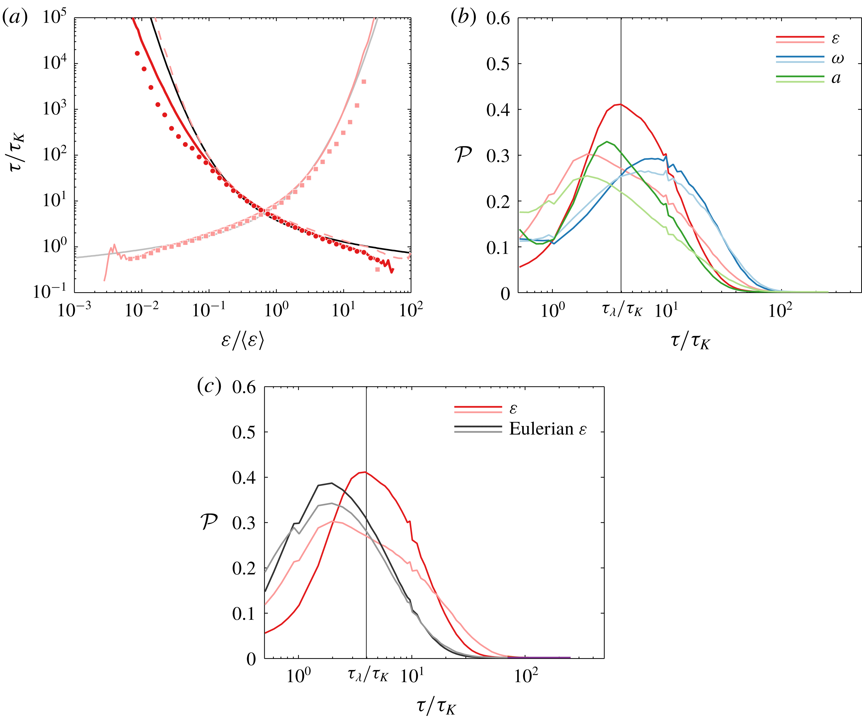
Profiles of mean flying and diving times
 $T_{F}(\unicode[STIX]{x1D700}_{t})$
and
 $T_{D}(\unicode[STIX]{x1D700}_{t})$
logically span a smaller range of magnitudes (figure 16
a) since the level of turbulence is weaker, however results stay consistent with those derived from the simulation at
 $Re_{\unicode[STIX]{x1D706}}=240$
and are accurately captured by our analytical approximations (6.7). Interestingly, as predicted by our model,
 $\unicode[STIX]{x1D700}_{t}^{s}$
slightly increases when decreasing
 $Re_{\unicode[STIX]{x1D706}}$
. Figure 16(c) shows the flying and diving LPDFs at
 $\unicode[STIX]{x1D711}_{t}^{s}$
. Results for dissipation are consistent with those at
 $Re_{\unicode[STIX]{x1D706}}=240$
with a most probable diving time at
 $2\unicode[STIX]{x1D70F}_{K}$
and flying time at the Taylor time scale
 $\unicode[STIX]{x1D70F}_{\unicode[STIX]{x1D706}}$
. On the contrary, one can observe a slight Reynolds number dependency for acceleration.
Eulerian flying and diving LPDFs could be computed with this dataset (figure 16 c). Results show that Eulerian intermittency tends to be faster than Lagrangian intermittency.