1 Introduction
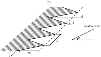
A theoretical model is proposed in this paper for the scattering of sound waves from a semi-infinite flat rigid plate with laterally periodic serrated open ends (see figure 1) in the presence of a uniform background flow. The sawtooth-shaped edge, which is formally known as a serration, has recently become a popular topic in the aerospace and avian research community (Chong et al. Reference Chong, Vathylakis, Joseph and Gruber2013; Chong & Joseph Reference Chong and Joseph2013; Narayanan et al. Reference Narayanan, Chaitanya, Haeri, Joseph, Kim and Polacsek2015) due to its presumed connection to the silent flying capability of owls (Lilley Reference Lilley1998; Jaworski & Peake Reference Jaworski and Peake2013). Further understanding of the underlying mechanisms will certainly provide new technological directions for low-noise aircraft designs that can eventually reduce the related environmental impact. Until now, the influence of the serrations has been studied mainly from the perspective of fluid dynamics (Howe Reference Howe1991b ; Jones & Sandberg Reference Jones and Sandberg2012), using either experimental (Chong et al. Reference Chong, Vathylakis, Joseph and Gruber2013) or numerical tools (Jones & Sandberg Reference Jones and Sandberg2012). Ayton & Peake (Reference Ayton and Peake2013) have developed a theoretical model for the scattered sound field when a sound wave is incident on an aerofoil. Recently, Stalnov, Chaitanya & Joseph (Reference Stalnov, Chaitanya and Joseph2016) have proposed a prediction model for aerofoil broadband self-noise. Both works consider aerofoils with straight trailing edges. Howe (Reference Howe1991b ) and Lyu, Azarpeyvand & Sinayoko (Reference Lyu, Azarpeyvand and Sinayoko2016) have proposed theoretical models for a flat-plate aerofoil with trailing-edge serrations, from which a wall pressure turbulent gust is scattered to far-field regions. Overall, theoretical models that illuminate the possible acoustic scattering from a serrated plate due to external incident sound waves are still rare. To address this issue, the current work endeavours to develop a theoretical model to study the scattering from serrations. The key contribution of this work is the analytic (and innovative) description of the acoustic scattering effect of serrations by incorporating Fourier series expansions and the Wiener–Hopf method.
The Wiener–Hopf method is a powerful mathematical tool which can yield closed-form analytical solutions for classical scattering problems such as diffraction from a rigid flat plate (Noble Reference Noble1958) and duct radiation (Munt Reference Munt1977; Rienstra Reference Rienstra1984; Gabard & Astley Reference Gabard and Astley2006; Veitch & Peake Reference Veitch and Peake2008; Liu et al. Reference Liu, Jiang, Huang and Chen2016). To take account of the serrated open ends, the current work further extends Noble’s classical model, which is also known as the rigid screen diffraction problem (Noble Reference Noble1958), by adopting the Fourier expansion concept proposed in a recent study (Liu et al. Reference Liu, Jiang, Huang and Chen2016). In particular, the periodic profiles of the serrations can be described by means of Fourier series that will accurately represent the geometrical layout of the periodic serrations in the lateral direction. Then, a Wiener–Hopf based theoretical model can be established to analytically examine the scattering waves from the serrated plate. The associated matrix Wiener–Hopf kernel can be derived and a rigorous closed-form solution will be eventually obtained. It will become clear later in this paper that the matrix kernel is diagonal and, therefore, its mathematical manipulation (i.e. the kernel factorisation) is already well known (Noble Reference Noble1958). Overall, the most difficult part of this work is the modelling of the current problem of interest in the theoretical Wiener–Hopf framework, which can mathematically elucidate the effect of the serrations as a convolution operation in the wavenumber domain.
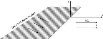
Sketch of the model problem. Here,
 $x,y,z$
are the coordinates,
 $O$
the origin,
 $\unicode[STIX]{x1D712}(z)$
the profile of serrations,
 $2h_{s}$
the root-to-tip distance and
 $\unicode[STIX]{x1D703}$
the incident angle.

A recent theoretical work (Lyu et al. Reference Lyu, Azarpeyvand and Sinayoko2016) has developed a noise prediction model for periodic sawtooth edges by means of Fourier series expansion. The modelling of the scattered field was treated by a straightforward generalisation of Schwarzschild’s technique for the Helmholtz equation with semi-infinite mixed boundary conditions. In particular, a sawtooth edge was transformed to an equivalent straight edge by a geometrical transformation. The resultant equation (Lyu et al. Reference Lyu, Azarpeyvand and Sinayoko2016, (2.11)) and the subsequent simplification are therefore solely for sawtooth-shaped serrations. In contrast, the current work incorporates Fourier expansions into the Wiener–Hopf method and should be applicable to many generic shapes. Both sawtooth and sinusoidal shapes will be investigated in the current study.
The pioneering work of Howe (Reference Howe1991a ,Reference Howe b ) and the recent theoretical model (Lyu et al. Reference Lyu, Azarpeyvand and Sinayoko2016) focused on the scattering effect due to serrations exclusively. All of these theoretical studies adopted a set-up with turbulent wall gusts in the vicinity of a serrated semi-infinite flat plate (Brooks & Hodgson Reference Brooks and Hodgson1981). Possible fluid mechanisms, such as a finite chord (Jeon & Lee Reference Jeon and Lee2008), aeroacoustic feedback (Jones & Sandberg Reference Jones and Sandberg2011, Reference Jones and Sandberg2012) and the hydrodynamic effect of trailing-edge serrations (Jones & Sandberg Reference Jones and Sandberg2012), will produce certain changes in the turbulence characteristics and scattered sound waves from serrations. Nevertheless, one of the most important assumptions made in the above theoretical works is the frozen turbulent wall gusts during their interactions with the downstream edges. This frozen turbulence approximation was presumably applicable to incident wall gusts at reasonably high frequencies with a much smaller wavelength than the serration dimensions. The current work considers the scattered field due to external sound waves impinging on a semi-infinite serrated plate, which seems to be a system that is acoustically related to these wall turbulence scattering problems (Howe Reference Howe1991b ; Lyu et al. Reference Lyu, Azarpeyvand and Sinayoko2016) (more detailed discussion can be found in appendix B). Hence, as will be shown later, the current model will produce the same conclusions regarding the possible noise control effects of the serrations. In addition, the current model will show that the serrations can excite on-surface scattered waves of regular lateral patterns more effectively at higher frequencies.
This paper is organised as follows. Section 2 will introduce the model set-up with a semi-infinite surface and serrations. Then, a theoretical model will be developed by incorporating the Wiener–Hopf method and Fourier series expansions. In § 3, a couple of numerical test cases will be performed with some representative set-ups to validate the proposed prediction model. Then, parametric studies and the associated discussion will be given. Finally, § 4 will summarise the present work. A brief extension to cases with a uniform mean flow can be found in appendix A. The Wiener–Hopf models for the scattering of boundary pressure gust and oncoming gust flows can be found in appendices B and C respectively.
2 The theoretical model
2.1 Statement of the problem
As shown in figure 1, the problem considered in this work contains an infinite number of periodic and straight (in the
 $x$
direction) serrations in the
 $z$
direction. Here, we only consider rigid serrations. For poroelastic edges, the interested reader can refer to recent experimental and theoretical works (Jaworski & Peake Reference Jaworski and Peake2013; Ayton Reference Ayton2016a
; Chong & Dubois Reference Chong and Dubois2016). The profile of the serrations is represented by
 $\unicode[STIX]{x1D712}(z)$
, which is mainly dependent on two geometrical parameters: the period
 $\unicode[STIX]{x1D706}$
and the root-to-tip distance
 $2h_{s}$
. The rest of the semi-infinite surface is assumed to be rigid and infinitely thin. For simplicity, a stationary background flow is assumed for the current work. Nevertheless, the theoretical model developed in this work can be easily extended to cases with uniform background flows by using the Prandtl–Glauert transformation (Huang, Zhong & Stalnov Reference Huang, Zhong and Stalnov2014b
) (a brief introduction is included in appendix A). For the current set-up, an incident wave coming from the far-field region with an incident angle
 $\unicode[STIX]{x1D703}$
will impinge on the serrated flat plate and further generate scattering waves.
Then, the governing wave equation for the current problem is
 $$\begin{eqnarray}\left(\frac{\unicode[STIX]{x2202}^{2}}{\unicode[STIX]{x2202}x^{2}}+\frac{\unicode[STIX]{x2202}^{2}}{\unicode[STIX]{x2202}y^{2}}+\frac{\unicode[STIX]{x2202}^{2}}{\unicode[STIX]{x2202}z^{2}}\right)\unicode[STIX]{x1D719}-\frac{\unicode[STIX]{x2202}^{2}}{\unicode[STIX]{x2202}t^{2}}\unicode[STIX]{x1D719}=0,\end{eqnarray}$$
where
 $\unicode[STIX]{x1D719}$
is the acoustic potential. All of the variables are non-dimensionalised using the reference length scale
 $\unicode[STIX]{x1D706}_{0}^{\ast }$
, which is the wavelength of the incident sound at
 $340~\text{Hz}$
, the density of air
 $\unicode[STIX]{x1D70C}_{0}^{\ast }=1.225~\text{kg}~\text{m}^{-3}$
and the speed of sound
 $c_{0}^{\ast }=340~\text{m}~\text{s}^{-1}$
.
From the acoustic potential
 $\unicode[STIX]{x1D719}$
, we will be able to obtain the sound pressure
 $p$
, the particle velocity
 $\boldsymbol{v}=(u,v,w)$
and the acoustic density
 $\unicode[STIX]{x1D70C}$
by using the following relations:
 $$\begin{eqnarray}p=p_{i}+p_{s}=-\frac{\unicode[STIX]{x2202}\unicode[STIX]{x1D719}}{\unicode[STIX]{x2202}t},\quad \boldsymbol{v}=\unicode[STIX]{x1D735}\unicode[STIX]{x1D719},\quad \unicode[STIX]{x1D70C}=p,\end{eqnarray}$$
where the subscripts
 $(\cdot )_{i}$
and
 $(\cdot )_{s}$
denote the incident and scattering waves respectively. Further, the incident wave from the far-field region presumably has a time-harmonic form,
 $$\begin{eqnarray}\unicode[STIX]{x1D719}_{i}(x,y,\unicode[STIX]{x1D703}\!,t)=\unicode[STIX]{x1D713}_{i}(x,y,\unicode[STIX]{x1D703})\text{e}^{-\text{i}\unicode[STIX]{x1D714}t}=A_{i}\text{e}^{-\text{i}k(x\cos \unicode[STIX]{x1D703}+y\sin \unicode[STIX]{x1D703})-\text{i}\unicode[STIX]{x1D714}t},\end{eqnarray}$$
where
 $A_{i}$
is the normalised amplitude of the incident wave,
 $k$
is the normalised wavenumber (hence,
 $k=\unicode[STIX]{x1D714}$
) and
 $\unicode[STIX]{x1D703}$
is the incident angle (see figure 1). For a linear wave system, the scattered field will also take the harmonic form
 $$\begin{eqnarray}\displaystyle \unicode[STIX]{x1D719}_{s}(x,y,z,t)=\unicode[STIX]{x1D713}_{s}(x,y,z)\text{e}^{-\text{i}\unicode[STIX]{x1D714}t}. & & \displaystyle\end{eqnarray}$$
For simplicity, the common factor
 $\exp (-\text{i}\unicode[STIX]{x1D714}t)$
will be omitted throughout the rest of this paper. Then,
 $\unicode[STIX]{x1D713}_{s}$
should satisfy the Helmholtz equation,
 $$\begin{eqnarray}\left(\frac{\unicode[STIX]{x2202}^{2}}{\unicode[STIX]{x2202}x^{2}}+\frac{\unicode[STIX]{x2202}^{2}}{\unicode[STIX]{x2202}y^{2}}+\frac{\unicode[STIX]{x2202}^{2}}{\unicode[STIX]{x2202}z^{2}}\right)\unicode[STIX]{x1D713}_{s}+k^{2}\unicode[STIX]{x1D713}_{s}=0,\end{eqnarray}$$
and further be subject to the following boundary conditions.
-
(1) Rigid plate condition.
On the rigid plate (where
 $v=0$
), the scattered field is equal but opposite to the incident field, resulting in (2.6)
$$\begin{eqnarray}\left.\frac{\unicode[STIX]{x2202}\unicode[STIX]{x1D713}_{s}\left(x,y,z\right)}{\unicode[STIX]{x2202}y}\right|_{y=0}=-\!\left.\frac{\unicode[STIX]{x2202}\unicode[STIX]{x1D713}_{i}\left(x,y,z\right)}{\unicode[STIX]{x2202}y}\right|_{y=0}=\text{i}k\sin \unicode[STIX]{x1D703}\cdot \text{e}^{-\text{i}kx\cos \unicode[STIX]{x1D703}},\quad \forall x\leqslant \unicode[STIX]{x1D712}(z).\end{eqnarray}$$
-
(2) The scattered field
$\unicode[STIX]{x1D713}_{s}$
should be an odd function in
$y$
and continuous for
$x>\unicode[STIX]{x1D712}(z)$
(Noble Reference Noble1958), hence (2.7)
$$\begin{eqnarray}\unicode[STIX]{x1D713}_{s}(x,y,z)|_{y=0}=0,\quad \forall x>\unicode[STIX]{x1D712}(z).\end{eqnarray}$$
-
(3) The far-field radiation condition and the edge condition.
Here, the theoretical model is developed for stationary mean flow cases. The edge condition is imposed at the serrated open ends to ensure a finite velocity potential at the edge and to obtain a unique solution of the problem (Munt Reference Munt1977; Gabard & Astley Reference Gabard and Astley2006). More specifically,
$\unicode[STIX]{x1D713}_{s}(x,0,z)\rightarrow \boldsymbol{O}((x-\unicode[STIX]{x1D712}(z))^{1/2})$
as
$x\rightarrow \unicode[STIX]{x1D712}(z)^{+}$
for a leading-edge case and
$\unicode[STIX]{x1D713}_{s}(x,0,z)\rightarrow \boldsymbol{O}((x-\unicode[STIX]{x1D712}(z))^{3/2})$
as
$x\rightarrow \unicode[STIX]{x1D712}(z)^{+}$
for a trailing-edge case. Here,
$\unicode[STIX]{x1D712}(z)^{+}$
denotes the positive side of
$\unicode[STIX]{x1D712}(z)$
in the
$x$
direction. This edge condition will ensure the desired algebraic property for solving the scattered sound field in the axial wavenumber domain. For turbulent gusts and aerofoil interactions, some more subtle studies may be required for the cases with a leading-edge stagnation point (Ayton Reference Ayton2016b
) or a trailing-edge unsteady Kutta condition (Ayton, Gill & Peake Reference Ayton, Gill and Peake2016).







We should emphasise that the primary focus of this model is the prediction of scattered wave fields from leading-edge serrations. The high-frequency self-noise, which is presumably due to the vortex shedding from serrations (Chong et al. Reference Chong, Vathylakis, Joseph and Gruber2013; Vathylakis, Chong & Joseph Reference Vathylakis, Chong and Joseph2015), is not considered in this work.
2.2 The Wiener–Hopf model
The essential concept behind this model is the incorporation of Fourier series expansions into the Wiener–Hopf method. The same concept has been successfully applied in one of our recent papers for sound propagation inside a cylindrical flow duct with rigid splices (Liu et al. Reference Liu, Jiang, Huang and Chen2016). The new difficulty for the current theoretical development comes from the representation of the serrated flat-plate problem in the framework of a Wiener–Hopf model with the desired analytic properties (especially the complex analytical properties on the upper and lower halves of the complex plane for the transformed scattered field from serrations).
The Wiener–Hopf method will enable us to obtain rigorous solutions for the wave equations with a pair of idealised but mixed boundary conditions. Typically, the first step of the Wiener–Hopf method is to transform the wave equations into Wiener–Hopf equations via Fourier transform. The next step is to decompose the associated Wiener–Hopf kernel by using suitable factorisation methods, which should yield decomposition results that are analytic and bounded on the upper- and lower-half complex planes respectively. Then, a closed-form solution will be available by applying Liouville’s theorem. More detailed developments for the current problem are given below.
First,
 $\unicode[STIX]{x1D713}_{s}$
is periodic in the
 $z$
direction and, therefore, can be represented as follows by using the Fourier series:
 $$\begin{eqnarray}\unicode[STIX]{x1D713}_{s}(x,y,z)=\mathop{\sum }_{\unicode[STIX]{x1D705}=-\infty }^{+\infty }\unicode[STIX]{x1D713}_{s}^{\unicode[STIX]{x1D705}}(x,y)\text{e}^{\text{i}\unicode[STIX]{x1D705}(2\unicode[STIX]{x03C0}/\unicode[STIX]{x1D706})z},\quad \unicode[STIX]{x1D713}_{s}^{\unicode[STIX]{x1D705}}(x,y)=\frac{1}{\unicode[STIX]{x1D706}}\int _{0}^{\unicode[STIX]{x1D706}}\unicode[STIX]{x1D713}_{s}(x,y,z)\text{e}^{-\text{i}\unicode[STIX]{x1D705}(2\unicode[STIX]{x03C0}/\unicode[STIX]{x1D706})z}\,\text{d}z,\end{eqnarray}$$
where
 $(\cdot )^{\unicode[STIX]{x1D705}}$
denotes the
 $\unicode[STIX]{x1D705}$
th component.
Substitution of (2.8) into (2.5) yields
 $$\begin{eqnarray}\left[\frac{\unicode[STIX]{x2202}^{2}}{\unicode[STIX]{x2202}x^{2}}+\frac{\unicode[STIX]{x2202}^{2}}{\unicode[STIX]{x2202}y^{2}}+k^{2}-\left(\unicode[STIX]{x1D705}\frac{2\unicode[STIX]{x03C0}}{\unicode[STIX]{x1D706}}\right)^{2}\right]\unicode[STIX]{x1D713}_{s}^{\unicode[STIX]{x1D705}}(x,y)=0.\end{eqnarray}$$
Then, the conventional Fourier transform is applied (in the
 $x$
direction) to the scattered acoustic field as follows:
 $$\begin{eqnarray}\displaystyle \unicode[STIX]{x1D6FD}(\unicode[STIX]{x1D6FC},y,z)\triangleq \int _{-\infty }^{+\infty }\unicode[STIX]{x1D713}_{s}(x,y,z)\text{e}^{\text{i}\unicode[STIX]{x1D6FC}x}\,\text{d}x=\int _{-\infty }^{+\infty }\left(\mathop{\sum }_{\unicode[STIX]{x1D705}=-\infty }^{+\infty }\unicode[STIX]{x1D713}_{s}^{\unicode[STIX]{x1D705}}(x,y)\text{e}^{\text{i}\unicode[STIX]{x1D705}(2\unicode[STIX]{x03C0}/\unicode[STIX]{x1D706})z}\right)\text{e}^{\text{i}\unicode[STIX]{x1D6FC}x}\,\text{d}x, & & \displaystyle\end{eqnarray}$$
where
 $\unicode[STIX]{x1D6FC}$
is the axial wavenumber. It is easy to see that
 $\unicode[STIX]{x1D6FD}(\unicode[STIX]{x1D6FC},y,z)$
is also periodic in the
 $z$
direction and, therefore, can be represented by the following Fourier series:
 $$\begin{eqnarray}\unicode[STIX]{x1D6FD}(\unicode[STIX]{x1D6FC},y,z)=\mathop{\sum }_{\unicode[STIX]{x1D705}=-\infty }^{+\infty }\unicode[STIX]{x1D6FD}^{\unicode[STIX]{x1D705}}(\unicode[STIX]{x1D6FC},y)\text{e}^{\text{i}\unicode[STIX]{x1D705}(2\unicode[STIX]{x03C0}/\unicode[STIX]{x1D706})z},\quad \unicode[STIX]{x1D6FD}^{\unicode[STIX]{x1D705}}(\unicode[STIX]{x1D6FC},y)=\int _{-\infty }^{+\infty }\unicode[STIX]{x1D713}_{s}^{\unicode[STIX]{x1D705}}(x,y)\text{e}^{\text{i}\unicode[STIX]{x1D6FC}x}\,\text{d}x.\end{eqnarray}$$
The latter relation assumes that the integration and the summation are commutative.
From (2.11), equation (2.9) can be transformed to
 $$\begin{eqnarray}\left\{\frac{\unicode[STIX]{x2202}^{2}}{\unicode[STIX]{x2202}y^{2}}-\left[\unicode[STIX]{x1D6FC}^{2}-\left(k^{2}-\left(\unicode[STIX]{x1D705}2\unicode[STIX]{x03C0}/\unicode[STIX]{x1D706}\right)^{2}\right)\right]\right\}\unicode[STIX]{x1D6FD}^{\unicode[STIX]{x1D705}}(\unicode[STIX]{x1D6FC},y)=0.\end{eqnarray}$$
To simplify the following formulations, we define
 ${\unicode[STIX]{x1D6FE}^{\unicode[STIX]{x1D705}}}^{2}\triangleq \unicode[STIX]{x1D6FC}^{2}-\hat{k^{\unicode[STIX]{x1D705}}}^{2}$
, with
 $\hat{k^{\unicode[STIX]{x1D705}}}^{2}\triangleq k^{2}-(\unicode[STIX]{x1D705}2\unicode[STIX]{x03C0}/\unicode[STIX]{x1D706})^{2}$
. To satisfy the radiation boundary condition, the solutions of (2.12) should have the following generic form:
 $$\begin{eqnarray}\unicode[STIX]{x1D6FD}^{\unicode[STIX]{x1D705}}(\unicode[STIX]{x1D6FC},y)=\left\{\begin{array}{@{}ll@{}}A^{\unicode[STIX]{x1D705}}(\unicode[STIX]{x1D6FC})\text{e}^{-\unicode[STIX]{x1D6FE}^{\unicode[STIX]{x1D705}}y},\quad \quad & \forall y>0,\\ -A^{\unicode[STIX]{x1D705}}(\unicode[STIX]{x1D6FC})\text{e}^{\unicode[STIX]{x1D6FE}^{\unicode[STIX]{x1D705}}y},\quad \quad & \forall y<0,\end{array}\right.\end{eqnarray}$$
where
 $A^{\unicode[STIX]{x1D705}}(\unicode[STIX]{x1D6FC})$
is the corresponding amplitude of the
 $\unicode[STIX]{x1D705}$
th component and
 $\unicode[STIX]{x1D6FE}^{\unicode[STIX]{x1D705}}$
is defined as a fractional power that will lead to a number of branch cuts joining the branch points
 $\pm \hat{k^{\unicode[STIX]{x1D705}}}$
to infinity. It is worthwhile to mention that
 $k$
is usually complex (with an additional small imaginary part, which will be set to zero in the final solution), so that
 $+\hat{k^{\unicode[STIX]{x1D705}}}$
and
 $-\hat{k^{\unicode[STIX]{x1D705}}}$
lie in the first and third quadrants of the complex
 $\unicode[STIX]{x1D6FC}$
-plane respectively (Munt Reference Munt1977). The setting of a small imaginary part of
 $k$
helps to ensure the causality of the final solutions, and the same technique has been adopted in many previous works (Rienstra Reference Rienstra1984; Gabard & Astley Reference Gabard and Astley2006; Liu et al.
Reference Liu, Jiang, Huang and Chen2016).
From (2.13), we further have the following relation at
 $y=0^{+}$
:
 $$\begin{eqnarray}\unicode[STIX]{x1D6FE}^{\unicode[STIX]{x1D705}}\unicode[STIX]{x1D6FD}^{\unicode[STIX]{x1D705}}(\unicode[STIX]{x1D6FC},0^{+})+{\unicode[STIX]{x1D6FD}^{\prime }}^{\unicode[STIX]{x1D705}}(\unicode[STIX]{x1D6FC},0^{+})=0,\quad \forall \unicode[STIX]{x1D705},\end{eqnarray}$$
where
 $(\cdot )^{\prime }$
represents
 $\text{d}/\text{d}y$
.
Now, we turn to the key part of this theoretical development. First, we decompose
 $\unicode[STIX]{x1D6FD}$
into the sum of the following two parts which are analytic on the two (yet unknown) half-planes:
 $$\begin{eqnarray}\displaystyle \unicode[STIX]{x1D6FD}(\unicode[STIX]{x1D6FC},y,z) & = & \displaystyle \text{e}^{\text{i}\unicode[STIX]{x1D6FC}\unicode[STIX]{x1D712}(z)}\left(\int _{\unicode[STIX]{x1D712}(z)}^{+\infty }\unicode[STIX]{x1D713}_{s}(x,y,z)\text{e}^{\text{i}\unicode[STIX]{x1D6FC}x-\text{i}\unicode[STIX]{x1D6FC}\unicode[STIX]{x1D712}(z)}\,\text{d}x+\int _{-\infty }^{\unicode[STIX]{x1D712}(z)}\unicode[STIX]{x1D713}_{s}(x,y,z)\text{e}^{\text{i}\unicode[STIX]{x1D6FC}x-\text{i}\unicode[STIX]{x1D6FC}\unicode[STIX]{x1D712}(z)}\,\text{d}x\right)\nonumber\\ \displaystyle & = & \displaystyle \text{e}^{\text{i}\unicode[STIX]{x1D6FC}\unicode[STIX]{x1D712}(z)}\left(\int _{0}^{+\infty }\unicode[STIX]{x1D713}_{s}(\hat{x}+\unicode[STIX]{x1D712}(z),y,z)\text{e}^{\text{i}\unicode[STIX]{x1D6FC}\hat{x}}\,\text{d}\hat{x}+\int _{-\infty }^{0}\unicode[STIX]{x1D713}_{s}(\hat{x}+\unicode[STIX]{x1D712}(z),y,z)\text{e}^{\text{i}\unicode[STIX]{x1D6FC}\hat{x}}\,\text{d}\hat{x}\right)\nonumber\\ \displaystyle & \triangleq & \displaystyle \text{e}^{\text{i}\unicode[STIX]{x1D6FC}\unicode[STIX]{x1D712}(z)}\left[\unicode[STIX]{x1D6FD}_{+}(\unicode[STIX]{x1D6FC},y,z)+\unicode[STIX]{x1D6FD}_{-}(\unicode[STIX]{x1D6FC},y,z)\right].\end{eqnarray}$$
In the whole theoretical development, the above equation is the most essential step, which ensures that the regularity of
 $\unicode[STIX]{x1D6FD}_{\pm }$
is independent of
 $\unicode[STIX]{x1D712}(z)$
and thus is consistent with the previous definitions in the classical flat-plate problem (Noble Reference Noble1958). In addition, the above definition actually suggests that
 $\unicode[STIX]{x1D712}(z)$
is a single-valued function, which should be satisfied for most representative set-ups.
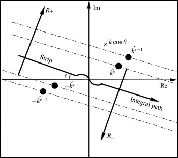
Argand diagram of the two complex half-planes
 $R_{\pm }$
and the overlapped strip. The symbol
 $\times$
denotes the pole at
 $k\cos \unicode[STIX]{x1D703}$
. For each
 $\unicode[STIX]{x1D705}$
, two branch cuts join the branch points
 $\pm \hat{k^{\unicode[STIX]{x1D705}}}$
to infinity through the two corresponding half-planes. Since
 $k$
is usually complex (Munt Reference Munt1977),
 $\pm \hat{k^{\unicode[STIX]{x1D705}}}$
and the corresponding branch cuts lie in the first and third quadrants of the complex plane (for clarity of this figure, the branch cuts are not shown here). The imaginary part is set to zero in the final solution and, hence, the integral path moves back to the horizontal axis with
 $\unicode[STIX]{x1D700}\rightarrow 0$
, except for a slight distortion (Rienstra Reference Rienstra1984; Gabard & Astley Reference Gabard and Astley2006) around the origin to avoid any possible singular point.

The decomposed
 $\unicode[STIX]{x1D6FD}_{\pm }$
are regular on the two overlapped half-planes, which are shown in figure 2. It is easy to see that
 $\exp (\text{i}\unicode[STIX]{x1D6FC}\unicode[STIX]{x1D712})$
,
 $\unicode[STIX]{x1D6FD}_{+}$
and
 $\unicode[STIX]{x1D6FD}_{-}$
in (2.15) are periodic in the
 $z$
direction with the same period
 $\unicode[STIX]{x1D706}$
. By expanding
 $\exp (\text{i}\unicode[STIX]{x1D6FC}\unicode[STIX]{x1D712})$
and
 $\unicode[STIX]{x1D6FD}_{\pm }$
into Fourier series, we immediately have
 $$\begin{eqnarray}\displaystyle \unicode[STIX]{x1D6FD}(\unicode[STIX]{x1D6FC},y,z)=\mathop{\sum }_{\unicode[STIX]{x1D705}_{1}=-\infty }^{+\infty }\unicode[STIX]{x1D701}^{\unicode[STIX]{x1D705}_{1}}\text{e}^{\text{i}\unicode[STIX]{x1D705}_{1}(2\unicode[STIX]{x03C0}/\unicode[STIX]{x1D706})z}\mathop{\sum }_{\unicode[STIX]{x1D705}_{2}=-\infty }^{+\infty }\left[\unicode[STIX]{x1D6FD}_{+}^{\unicode[STIX]{x1D705}_{2}}(\unicode[STIX]{x1D6FC},y)+\unicode[STIX]{x1D6FD}_{-}^{\unicode[STIX]{x1D705}_{2}}(\unicode[STIX]{x1D6FC},y)\right]\text{e}^{\text{i}\unicode[STIX]{x1D705}_{2}(2\unicode[STIX]{x03C0}/\unicode[STIX]{x1D706})z}, & & \displaystyle\end{eqnarray}$$
where
 $$\begin{eqnarray}\text{e}^{\text{i}\unicode[STIX]{x1D6FC}\unicode[STIX]{x1D712}(z)}=\mathop{\sum }_{\unicode[STIX]{x1D705}=-\infty }^{+\infty }\unicode[STIX]{x1D701}^{\unicode[STIX]{x1D705}}(\unicode[STIX]{x1D6FC})\text{e}^{\text{i}\unicode[STIX]{x1D705}(2\unicode[STIX]{x03C0}/\unicode[STIX]{x1D706})z},\quad \unicode[STIX]{x1D701}^{\unicode[STIX]{x1D705}}(\unicode[STIX]{x1D6FC})=\frac{1}{\unicode[STIX]{x1D706}}\int _{0}^{\unicode[STIX]{x1D706}}\text{e}^{\text{i}\unicode[STIX]{x1D6FC}\unicode[STIX]{x1D712}(z)}\text{e}^{-\text{i}\unicode[STIX]{x1D705}(2\unicode[STIX]{x03C0}/\unicode[STIX]{x1D706})z}\,\text{d}z,\end{eqnarray}$$
 $$\begin{eqnarray}\unicode[STIX]{x1D6FD}_{\pm }(\unicode[STIX]{x1D6FC},y,z)=\mathop{\sum }_{\unicode[STIX]{x1D705}=-\infty }^{+\infty }\unicode[STIX]{x1D6FD}_{\pm }^{\unicode[STIX]{x1D705}}(\unicode[STIX]{x1D6FC},y)\text{e}^{\text{i}\unicode[STIX]{x1D705}(2\unicode[STIX]{x03C0}/\unicode[STIX]{x1D706})z},\quad \unicode[STIX]{x1D6FD}_{\pm }^{\unicode[STIX]{x1D705}}(\unicode[STIX]{x1D6FC},y)=\frac{1}{\unicode[STIX]{x1D706}}\int _{0}^{\unicode[STIX]{x1D706}}\unicode[STIX]{x1D6FD}_{\pm }(\unicode[STIX]{x1D6FC},y,z)\text{e}^{-\text{i}\unicode[STIX]{x1D705}(2\unicode[STIX]{x03C0}/\unicode[STIX]{x1D706})z}\,\text{d}z.\end{eqnarray}$$
We should mention that
 $\unicode[STIX]{x1D6FC}$
in (2.17) may contain a small but non-zero imaginary part to ensure causality (details can be found in Gabard & Astley (Reference Gabard and Astley2006), Appendix A. Numerical methods). However, a Fourier series expansion is still available as long as
 $\unicode[STIX]{x1D712}(z)$
is periodic.
From (2.18), we can further define the partial derivatives with respect to
 $y$
for the
 $\unicode[STIX]{x1D705}$
th component:
 $$\begin{eqnarray}\unicode[STIX]{x1D6FD}_{\pm }^{\prime }(\unicode[STIX]{x1D6FC},y,z)=\mathop{\sum }_{\unicode[STIX]{x1D705}=-\infty }^{+\infty }{\unicode[STIX]{x1D6FD}_{\pm }^{\prime }}^{\unicode[STIX]{x1D705}}(\unicode[STIX]{x1D6FC},y)\text{e}^{\text{i}\unicode[STIX]{x1D705}(2\unicode[STIX]{x03C0}/\unicode[STIX]{x1D706})z}.\end{eqnarray}$$
From the hard-wall boundary condition (2.6), we can analytically represent
 $\unicode[STIX]{x1D6FD}_{-}^{\prime }(\unicode[STIX]{x1D6FC},0^{+},z)$
as follows:
 $$\begin{eqnarray}\displaystyle \unicode[STIX]{x1D6FD}_{-}^{\prime }(\unicode[STIX]{x1D6FC},0^{+},z) & = & \displaystyle \int _{-\infty }^{0}\unicode[STIX]{x1D713}_{s}^{\prime }(\hat{x}+\unicode[STIX]{x1D712}(z),0^{+},z)\text{e}^{\text{i}\unicode[STIX]{x1D6FC}\hat{x}}\,\text{d}\hat{x}\nonumber\\ \displaystyle & = & \displaystyle \int _{-\infty }^{0}\text{i}k\sin \unicode[STIX]{x1D703}\text{e}^{-\text{i}k\cos \unicode[STIX]{x1D703}(\hat{x}+\unicode[STIX]{x1D712})}\text{e}^{\text{i}\unicode[STIX]{x1D6FC}\hat{x}}\,\text{d}\hat{x}\nonumber\\ \displaystyle & = & \displaystyle \frac{k\sin \unicode[STIX]{x1D703}}{\unicode[STIX]{x1D6FC}-k\cos \unicode[STIX]{x1D703}}\text{e}^{-\text{i}k\unicode[STIX]{x1D712}(z)\cos \unicode[STIX]{x1D703}}=\frac{k\sin \unicode[STIX]{x1D703}}{\unicode[STIX]{x1D6FC}-k\cos \unicode[STIX]{x1D703}}\mathop{\sum }_{\unicode[STIX]{x1D705}=-\infty }^{+\infty }\unicode[STIX]{x1D710}^{\unicode[STIX]{x1D705}}\text{e}^{\text{i}\unicode[STIX]{x1D705}(2\unicode[STIX]{x03C0}/\unicode[STIX]{x1D706})z},\end{eqnarray}$$
with the Fourier series coefficients
 $$\begin{eqnarray}\unicode[STIX]{x1D710}^{\unicode[STIX]{x1D705}}=\frac{1}{\unicode[STIX]{x1D706}}\int _{0}^{\unicode[STIX]{x1D706}}\text{e}^{-\text{i}k\unicode[STIX]{x1D712}(z)\cos \unicode[STIX]{x1D703}}\text{e}^{-\text{i}\unicode[STIX]{x1D705}(2\unicode[STIX]{x03C0}/\unicode[STIX]{x1D706})z}\,\text{d}z,\end{eqnarray}$$
which mathematically represents the effect of different profile shapes of the serrations on the scattering of the incident waves. By comparing (2.19) and (2.20), it is easy to see that
 $$\begin{eqnarray}{\unicode[STIX]{x1D6FD}_{-}^{\prime }}^{\unicode[STIX]{x1D705}}(\unicode[STIX]{x1D6FC},0^{+})=\frac{k\sin \unicode[STIX]{x1D703}}{\unicode[STIX]{x1D6FC}-k\cos \unicode[STIX]{x1D703}}\unicode[STIX]{x1D710}^{\unicode[STIX]{x1D705}}.\end{eqnarray}$$
Next, by equating the terms of the same exponential orders in (2.16) and (2.11), we have the following relation:
 $$\begin{eqnarray}\displaystyle \unicode[STIX]{x1D6FD}^{\unicode[STIX]{x1D705}}(\unicode[STIX]{x1D6FC},y) & = & \displaystyle \cdots +\unicode[STIX]{x1D701}^{1}(\unicode[STIX]{x1D6FD}_{+}^{\unicode[STIX]{x1D705}-1}+\unicode[STIX]{x1D6FD}_{-}^{\unicode[STIX]{x1D705}-1})+\unicode[STIX]{x1D701}^{0}(\unicode[STIX]{x1D6FD}_{+}^{\unicode[STIX]{x1D705}}+\unicode[STIX]{x1D6FD}_{-}^{\unicode[STIX]{x1D705}})+\unicode[STIX]{x1D701}^{-1}(\unicode[STIX]{x1D6FD}_{+}^{\unicode[STIX]{x1D705}+1}+\unicode[STIX]{x1D6FD}_{-}^{\unicode[STIX]{x1D705}+1})+\cdots \nonumber\\ \displaystyle & = & \displaystyle \mathop{\sum }_{\unicode[STIX]{x1D705}_{2}=-\infty }^{+\infty }\unicode[STIX]{x1D701}^{\unicode[STIX]{x1D705}_{2}}(\unicode[STIX]{x1D6FD}_{+}^{\unicode[STIX]{x1D705}-\unicode[STIX]{x1D705}_{2}}(\unicode[STIX]{x1D6FC},y)+\unicode[STIX]{x1D6FD}_{-}^{\unicode[STIX]{x1D705}-\unicode[STIX]{x1D705}_{2}}(\unicode[STIX]{x1D6FC},y)).\end{eqnarray}$$
On substituting the boundary conditions at
 $y=0^{+}$
, i.e. equations (2.7) and (2.22), into (2.23), we have
 $$\begin{eqnarray}\displaystyle & \displaystyle \unicode[STIX]{x1D6FD}^{\unicode[STIX]{x1D705}}(\unicode[STIX]{x1D6FC},0^{+})=\mathop{\sum }_{\unicode[STIX]{x1D705}_{2}=-\infty }^{+\infty }\unicode[STIX]{x1D701}^{\unicode[STIX]{x1D705}_{2}}\unicode[STIX]{x1D6FD}_{-}^{\unicode[STIX]{x1D705}-\unicode[STIX]{x1D705}_{2}}(\unicode[STIX]{x1D6FC},0^{+}), & \displaystyle\end{eqnarray}$$
 $$\begin{eqnarray}\displaystyle & \displaystyle {\unicode[STIX]{x1D6FD}^{\prime }}^{\unicode[STIX]{x1D705}}(\unicode[STIX]{x1D6FC},0^{+})=\mathop{\sum }_{\unicode[STIX]{x1D705}_{2}=-\infty }^{+\infty }\unicode[STIX]{x1D701}^{\unicode[STIX]{x1D705}_{2}}\left({\unicode[STIX]{x1D6FD}_{+}^{\prime }}^{\unicode[STIX]{x1D705}-\unicode[STIX]{x1D705}_{2}}(\unicode[STIX]{x1D6FC},0^{+})+\frac{k\sin \unicode[STIX]{x1D703}}{\unicode[STIX]{x1D6FC}-k\cos \unicode[STIX]{x1D703}}\unicode[STIX]{x1D710}^{\unicode[STIX]{x1D705}-\unicode[STIX]{x1D705}_{2}}\right), & \displaystyle\end{eqnarray}$$
where
 $\unicode[STIX]{x1D6FD}_{-}(\unicode[STIX]{x1D6FC},0^{+})$
is always zero due to (2.7) and is thus omitted in (2.24). The above two equations should illuminate the mechanisms of the serrations in noise control. The right-hand side of (2.25) is actually a convolution of
 $\unicode[STIX]{x1D701}$
, which is only dependent on
 $\unicode[STIX]{x1D712}(z)$
. Mathematically, in the complex
 $\unicode[STIX]{x1D6FC}$
-plane, the scattered field is a convolution from the serrations. For brevity, the input variables
 $(\unicode[STIX]{x1D6FC},0^{+})$
will be omitted in the rest of this paper when no confusion will arise.
Substitution of (2.24) and (2.25) into (2.14) results in
 $$\begin{eqnarray}\unicode[STIX]{x1D6FE}^{\unicode[STIX]{x1D705}}\mathop{\sum }_{\unicode[STIX]{x1D705}_{2}=-\infty }^{+\infty }\unicode[STIX]{x1D701}^{\unicode[STIX]{x1D705}_{2}}\unicode[STIX]{x1D6FD}_{-}^{\unicode[STIX]{x1D705}-\unicode[STIX]{x1D705}_{2}}+\mathop{\sum }_{\unicode[STIX]{x1D705}_{2}=-\infty }^{+\infty }\unicode[STIX]{x1D701}^{\unicode[STIX]{x1D705}_{2}}{\unicode[STIX]{x1D6FD}_{+}^{\prime }}^{\unicode[STIX]{x1D705}-\unicode[STIX]{x1D705}_{2}}=-\frac{k\sin \unicode[STIX]{x1D703}}{\unicode[STIX]{x1D6FC}-k\cos \unicode[STIX]{x1D703}}\mathop{\sum }_{\unicode[STIX]{x1D705}_{2}=-\infty }^{+\infty }\unicode[STIX]{x1D701}^{\unicode[STIX]{x1D705}_{2}}\unicode[STIX]{x1D710}^{\unicode[STIX]{x1D705}-\unicode[STIX]{x1D705}_{2}}.\end{eqnarray}$$
By repeating (2.26) for all possible values of
 $\unicode[STIX]{x1D705}$
, we have a system of infinite linear equations which can be represented using the following matrix form:
 $$\begin{eqnarray}\unicode[STIX]{x1D6E4}\unicode[STIX]{x1D729}\unicode[STIX]{x1D6F7}_{-}+\unicode[STIX]{x1D729}\unicode[STIX]{x1D6F7}_{+}^{\prime }=\frac{-k\sin \unicode[STIX]{x1D703}}{\unicode[STIX]{x1D6FC}-k\cos \unicode[STIX]{x1D703}}\unicode[STIX]{x1D729}\unicode[STIX]{x1D730},\end{eqnarray}$$
where
 $$\begin{eqnarray}\displaystyle & \displaystyle \unicode[STIX]{x1D6E4}=\text{diag}(\unicode[STIX]{x1D6FE}^{\unicode[STIX]{x1D705}})=\text{diag}\left(\sqrt{\unicode[STIX]{x1D6FC}+\hat{k^{\unicode[STIX]{x1D705}}}}\sqrt{\unicode[STIX]{x1D6FC}-\hat{k^{\unicode[STIX]{x1D705}}}}\right)\triangleq \unicode[STIX]{x1D6E4}_{+}\unicode[STIX]{x1D6E4}_{-}, & \displaystyle\end{eqnarray}$$
 $$\begin{eqnarray}\displaystyle & \displaystyle \unicode[STIX]{x1D729}=\left[\begin{array}{@{}ccccccc@{}} & & & \cdots \, & & & \\ \cdots \, & \unicode[STIX]{x1D701}^{1} & \unicode[STIX]{x1D701}^{0} & \unicode[STIX]{x1D701}^{-1} & \cdots \, & & \\ & \cdots \, & \unicode[STIX]{x1D701}^{1} & \unicode[STIX]{x1D701}^{0} & \unicode[STIX]{x1D701}^{-1} & \cdots \, & \\ & & \cdots \, & \unicode[STIX]{x1D701}^{1} & \unicode[STIX]{x1D701}^{0} & \unicode[STIX]{x1D701}^{-1} & \cdots \\ & & & \cdots \, & & & \end{array}\right], & \displaystyle\end{eqnarray}$$
 $$\begin{eqnarray}\displaystyle & \displaystyle \unicode[STIX]{x1D6F7}_{-}=[\ldots ,\unicode[STIX]{x1D6FD}_{-}^{\unicode[STIX]{x1D705}-1},\unicode[STIX]{x1D6FD}_{-}^{\unicode[STIX]{x1D705}},\unicode[STIX]{x1D6FD}_{-}^{\unicode[STIX]{x1D705}+1},\ldots ]^{\text{T}}, & \displaystyle\end{eqnarray}$$
 $$\begin{eqnarray}\displaystyle & \displaystyle {\unicode[STIX]{x1D6F7}_{+}}^{\prime }=[\ldots ,{\unicode[STIX]{x1D6FD}_{+}^{\prime }}^{\unicode[STIX]{x1D705}-1},{\unicode[STIX]{x1D6FD}_{+}^{\prime }}^{\unicode[STIX]{x1D705}},{\unicode[STIX]{x1D6FD}_{+}^{\prime }}^{\unicode[STIX]{x1D705}+1},\ldots ]^{\text{T}}, & \displaystyle\end{eqnarray}$$
 $$\begin{eqnarray}\displaystyle & \displaystyle \unicode[STIX]{x1D730}=[\ldots ,\unicode[STIX]{x1D710}^{\unicode[STIX]{x1D705}-1},\unicode[STIX]{x1D710}^{\unicode[STIX]{x1D705}},\unicode[STIX]{x1D710}^{\unicode[STIX]{x1D705}+1},\ldots ]^{\text{T}}, & \displaystyle\end{eqnarray}$$
where
 $(\cdot )^{\text{T}}$
denotes the transpose operation,
 $\unicode[STIX]{x1D701}^{\unicode[STIX]{x1D705}}$
is defined in (2.17) and
 $\unicode[STIX]{x1D710}^{\unicode[STIX]{x1D705}}$
is defined in (2.21). In a practical implementation, the above infinite Wiener–Hopf matrix system is truncated to a finite dimension (Veitch & Peake Reference Veitch and Peake2008). The author has conducted convergence tests by examining the order of Fourier series
 $\unicode[STIX]{x1D705}$
in between
 $\pm 21$
, and found that values smaller than 21 could be sufficient as long as the corresponding finite summation of
 $\unicode[STIX]{x1D712}(z)$
converges satisfactorily. Hence, all of the results in the next section are calculated using
 $\unicode[STIX]{x1D705}\in [-10,10]$
.
After this truncation, it is straightforward to define a matrix inverse and the poles of
 $\unicode[STIX]{x1D729}$
. First, to achieve the Wiener–Hopf equation, equation (2.27) can be further simplified to
 $$\begin{eqnarray}\unicode[STIX]{x1D729}^{-1}\unicode[STIX]{x1D6E4}\unicode[STIX]{x1D729}\unicode[STIX]{x1D6F7}_{-}+\unicode[STIX]{x1D6F7}_{+}^{\prime }=\frac{-k\sin \unicode[STIX]{x1D703}}{\unicode[STIX]{x1D6FC}-k\cos \unicode[STIX]{x1D703}}\unicode[STIX]{x1D730}.\end{eqnarray}$$
As suggested by (2.16), the truncated matrices
 $\unicode[STIX]{x1D729}$
and
 $\unicode[STIX]{x1D729}^{-1}$
may contain entries that are polynomials in
 $\unicode[STIX]{x1D6FC}$
. Mathematically, the poles of a polynomial matrix are the roots of
 $\det \mathfrak{D}(\unicode[STIX]{x1D6FC})=0$
, where
 $\mathfrak{D}$
is the denominator of the coprime matrix fraction descriptions of the polynomial matrix. The poles can also be simply calculated as the union of the poles for each entry of a matrix. This simple treatment has been adopted in some commercial software such as MATLAB® and is also used in this work. On the other hand, for either sawtooth- or sinusoidal-shaped serrations, it is easy to prove that each entry of the corresponding
 $\unicode[STIX]{x1D729}$
(or
 $\unicode[STIX]{x1D729}^{-1}$
) is analytic because the real and imaginary parts of
 $\unicode[STIX]{x1D729}$
(and
 $\unicode[STIX]{x1D729}^{-1}$
) satisfy the Cauchy–Riemann equations. For other possible profiles of the serrations, the corresponding
 $\unicode[STIX]{x1D729}$
may still have a number of unknown poles and zeros (i.e. poles for
 $\unicode[STIX]{x1D729}^{-1}$
) at
 $\unicode[STIX]{x1D6FC}_{j}$
, and, therefore, neither
 $\unicode[STIX]{x1D729}$
nor
 $\unicode[STIX]{x1D729}^{-1}$
satisfies the analytic condition, which is most essential in the Wiener–Hopf method. To cancel out these poles, the term of
 $[\unicode[STIX]{x1D6F1}(\unicode[STIX]{x1D6FC}-\unicode[STIX]{x1D6FC}_{j})]^{-1}\unicode[STIX]{x1D6F1}(\unicode[STIX]{x1D6FC}-\unicode[STIX]{x1D6FC}_{j})$
is multiplied to both sides of (2.33), resulting in
 $$\begin{eqnarray}\underbrace{[\unicode[STIX]{x1D729}^{-1}\unicode[STIX]{x1D6F1}(\unicode[STIX]{x1D6FC}-\unicode[STIX]{x1D6FC}_{j})^{-1}]}_{\hat{\unicode[STIX]{x1D729}}^{-1}}\unicode[STIX]{x1D6E4}\underbrace{[\unicode[STIX]{x1D6F1}(\unicode[STIX]{x1D6FC}-\unicode[STIX]{x1D6FC}_{j})\unicode[STIX]{x1D729}]}_{\hat{\unicode[STIX]{x1D729}}}\unicode[STIX]{x1D6F7}_{-}+\unicode[STIX]{x1D6F7}_{+}^{\prime }=\frac{-k\sin \unicode[STIX]{x1D703}}{\unicode[STIX]{x1D6FC}-k\cos \unicode[STIX]{x1D703}}\unicode[STIX]{x1D730},\end{eqnarray}$$
where
 $\unicode[STIX]{x1D6F1}$
represents the product of a sequence of
 $(\unicode[STIX]{x1D6FC}-\unicode[STIX]{x1D6FC}_{j})$
. By the above multiplication, the poles of
 $\unicode[STIX]{x1D729}$
and
 $\unicode[STIX]{x1D729}^{-1}$
can be cancelled. Then,
 $\hat{\unicode[STIX]{x1D729}}$
and
 $\hat{\unicode[STIX]{x1D729}}^{-1}$
in (2.34) become analytic. It will become clear that the above multiplication operation is only for the rigour of the whole theoretical development and is not required in the actual implementation, since the term
 $[\unicode[STIX]{x1D6F1}(\unicode[STIX]{x1D6FC}-\unicode[STIX]{x1D6FC}_{j})]^{-1}\unicode[STIX]{x1D6F1}(\unicode[STIX]{x1D6FC}-\unicode[STIX]{x1D6FC}_{j})$
itself equals 1.
It can be seen that (2.34) still contains two unknowns,
 $\unicode[STIX]{x1D6F7}_{+}^{\prime }$
and
 $\unicode[STIX]{x1D6F7}_{-}$
. To solve this equation, the Wiener–Hopf method should be considered. First,
 $\unicode[STIX]{x1D6E4}$
is a diagonal matrix and its multiplicative factorisation satisfying
 $\unicode[STIX]{x1D6E4}=\unicode[STIX]{x1D6E4}_{+}\unicode[STIX]{x1D6E4}_{-}$
can be easily obtained (see (2.28)). Then,
 $$\begin{eqnarray}\unicode[STIX]{x1D6E4}_{-}(\unicode[STIX]{x1D6FC})\hat{\unicode[STIX]{x1D729}}\unicode[STIX]{x1D6F7}_{-}+\unicode[STIX]{x1D6E4}_{+}^{-1}(\unicode[STIX]{x1D6FC})\hat{\unicode[STIX]{x1D729}}\unicode[STIX]{x1D6F7}_{+}^{\prime }=\frac{-k\sin \unicode[STIX]{x1D703}}{\unicode[STIX]{x1D6FC}-k\cos \unicode[STIX]{x1D703}}\unicode[STIX]{x1D6E4}_{+}^{-1}(\unicode[STIX]{x1D6FC})\hat{\unicode[STIX]{x1D729}}\unicode[STIX]{x1D730}.\end{eqnarray}$$
By rearranging terms and cancelling out the pole at
 $k\cos \unicode[STIX]{x1D703}$
, we finally achieve the following Wiener–Hopf equation:
 $$\begin{eqnarray}\displaystyle & & \displaystyle \underbrace{\unicode[STIX]{x1D6E4}_{-}(\unicode[STIX]{x1D6FC})\hat{\unicode[STIX]{x1D729}}\unicode[STIX]{x1D6F7}_{-}+\frac{k\sin \unicode[STIX]{x1D703}}{\unicode[STIX]{x1D6FC}-k\cos \unicode[STIX]{x1D703}}\unicode[STIX]{x1D6E4}_{+}^{-1}(k\cos \unicode[STIX]{x1D703})\hat{\unicode[STIX]{x1D729}}\unicode[STIX]{x1D730}}_{R_{-}}\nonumber\\ \displaystyle & & \displaystyle \quad =-\!\underbrace{\unicode[STIX]{x1D6E4}_{+}^{-1}(\unicode[STIX]{x1D6FC})\hat{\unicode[STIX]{x1D729}}\unicode[STIX]{x1D6F7}_{+}^{\prime }-\frac{k\sin \unicode[STIX]{x1D703}}{\unicode[STIX]{x1D6FC}-k\cos \unicode[STIX]{x1D703}}[\unicode[STIX]{x1D6E4}_{+}^{-1}(\unicode[STIX]{x1D6FC})-\unicode[STIX]{x1D6E4}_{+}^{-1}(k\cos \unicode[STIX]{x1D703})]\hat{\unicode[STIX]{x1D729}}\unicode[STIX]{x1D730}}_{R_{+}}\equiv \boldsymbol{E}(\unicode[STIX]{x1D6FC}).\quad\end{eqnarray}$$
2.3 The analytical solutions
The left- and right-hand sides of (2.36) should be regular on the positive and negative half-planes
 $R_{\pm }$
respectively, where
 $R_{+}$
is the positive half-plane above all possible
 $-\hat{k^{\unicode[STIX]{x1D705}}}$
, and
 $R_{-}$
is the negative half-plane below all possible
 $\hat{k^{\unicode[STIX]{x1D705}}}$
and
 $k\cos \unicode[STIX]{x1D703}$
(see figure 2). Both
 $R_{+}$
and
 $R_{-}$
will share an overlapped region. As a result, according to analytic continuation in the complex analysis theory,
 $\boldsymbol{E}(\unicode[STIX]{x1D6FC})$
is an entire function that is regular on the whole complex
 $\unicode[STIX]{x1D6FC}$
-plane. By considering the classical case with a flat rigid plate, it can be shown that
 $\boldsymbol{E}(\unicode[STIX]{x1D6FC})\equiv 0$
as
 $|\unicode[STIX]{x1D6FC}|\rightarrow \infty$
. In addition, it is very easy to see that the edge condition will also force
 $\boldsymbol{E}(\unicode[STIX]{x1D6FC})\equiv 0$
as
 $|\unicode[STIX]{x1D6FC}|\rightarrow \infty$
. Otherwise, the finiteness of the scattering wave at the edge (where
 $\unicode[STIX]{x1D712}(z)=0$
) will be violated. However, the problem becomes more complicated for serrated ends with
 $\unicode[STIX]{x1D712}(z)\neq 0$
. With no loss of generality, we assume
 $\unicode[STIX]{x1D712}(z)\geqslant 0$
. Then, it is easy to prove that each element in
 $\hat{\unicode[STIX]{x1D729}}$
,
 $$\begin{eqnarray}\unicode[STIX]{x1D701}^{\unicode[STIX]{x1D705}}(\unicode[STIX]{x1D6FC})=\frac{1}{\unicode[STIX]{x1D706}}\int _{0}^{\unicode[STIX]{x1D706}}\text{e}^{\text{i}\unicode[STIX]{x1D6FC}\unicode[STIX]{x1D712}(z)}\text{e}^{-\text{i}\unicode[STIX]{x1D705}(2\unicode[STIX]{x03C0}/\unicode[STIX]{x1D706})z}\,\text{d}z,\end{eqnarray}$$
is analytic but unbounded in the half-plane
 $R_{-}$
(when the imaginary part of
 $\unicode[STIX]{x1D6FC}$
approaches
 $-\infty$
). To apply Liouville’s theorem (for an analytic and bounded function), we should modify (2.34) to
 $$\begin{eqnarray}\underbrace{\hat{\unicode[STIX]{x1D729}}^{-1}\unicode[STIX]{x1D6E4}_{+}\hat{\unicode[STIX]{x1D729}}}_{\boldsymbol{K}_{+}}\underbrace{\hat{\unicode[STIX]{x1D729}}^{-1}\unicode[STIX]{x1D6E4}_{-}\hat{\unicode[STIX]{x1D729}}}_{\boldsymbol{K}_{-}}\unicode[STIX]{x1D6F7}_{-}+\unicode[STIX]{x1D6F7}_{+}^{\prime }=\frac{-k\sin \unicode[STIX]{x1D703}}{\unicode[STIX]{x1D6FC}-k\cos \unicode[STIX]{x1D703}}\unicode[STIX]{x1D730},\end{eqnarray}$$
which results in
 $$\begin{eqnarray}\displaystyle & & \displaystyle \underbrace{\displaystyle \boldsymbol{K}_{-}(\unicode[STIX]{x1D6FC})\unicode[STIX]{x1D6F7}_{-}(\unicode[STIX]{x1D6FC})+\frac{k\sin \unicode[STIX]{x1D703}}{\unicode[STIX]{x1D6FC}-k\cos \unicode[STIX]{x1D703}}\hat{\unicode[STIX]{x1D729}}^{-1}(\unicode[STIX]{x1D6FC})\unicode[STIX]{x1D6E4}_{+}^{-1}(k\cos \unicode[STIX]{x1D703})\hat{\unicode[STIX]{x1D729}}(\unicode[STIX]{x1D6FC})\unicode[STIX]{x1D730}(\unicode[STIX]{x1D6FC})}_{R_{-}}\nonumber\\ \displaystyle & & \displaystyle \quad =-\!\underbrace{\displaystyle \boldsymbol{K}_{+}^{-1}(\unicode[STIX]{x1D6FC})\unicode[STIX]{x1D6F7}_{+}^{\prime }(\unicode[STIX]{x1D6FC})-\frac{k\sin \unicode[STIX]{x1D703}}{\unicode[STIX]{x1D6FC}-k\cos \unicode[STIX]{x1D703}}\hat{\unicode[STIX]{x1D729}}^{-1}(\unicode[STIX]{x1D6FC})\left[\unicode[STIX]{x1D6E4}_{+}^{-1}(\unicode[STIX]{x1D6FC})-\unicode[STIX]{x1D6E4}_{+}^{-1}(k\cos \unicode[STIX]{x1D703})\right]\hat{\unicode[STIX]{x1D729}}(\unicode[STIX]{x1D6FC})\unicode[STIX]{x1D730}(\unicode[STIX]{x1D6FC})}_{R_{+}}.\nonumber\\ \displaystyle & & \displaystyle\end{eqnarray}$$
It should be straightforward to prove that the left- and right-hand sides of (2.39) are analytic and bounded in
 $R_{-}$
and
 $R_{+}$
respectively. Then, we can achieve the final solution by the following steps. First, by applying analytic continuation, a single function
 $\boldsymbol{E}(\unicode[STIX]{x1D6FC})$
that is regular on the whole complex
 $\unicode[STIX]{x1D6FC}$
-plane can be defined from (2.39). Second, by Liouville’s theorem, this bounded entire function must be a constant. Then, by studying the behaviour of
 $\boldsymbol{E}(\unicode[STIX]{x1D6FC})$
as
 $|\unicode[STIX]{x1D6FC}|$
approaches
 $\infty$
, we have
 $\boldsymbol{E}(\unicode[STIX]{x1D6FC})\equiv 0$
. Finally, by substituting
 $\boldsymbol{E}(\unicode[STIX]{x1D6FC})\equiv 0$
into (2.39), we have
 $$\begin{eqnarray}\displaystyle \unicode[STIX]{x1D6F7}_{-}(\unicode[STIX]{x1D6FC}) & = & \displaystyle -\boldsymbol{K}_{-}^{-1}(\unicode[STIX]{x1D6FC})\frac{k\sin \unicode[STIX]{x1D703}}{\unicode[STIX]{x1D6FC}-k\cos \unicode[STIX]{x1D703}}\hat{\unicode[STIX]{x1D729}}^{-1}(\unicode[STIX]{x1D6FC})\unicode[STIX]{x1D6E4}_{+}^{-1}(k\cos \unicode[STIX]{x1D703})\hat{\unicode[STIX]{x1D729}}(\unicode[STIX]{x1D6FC})\unicode[STIX]{x1D730}(\unicode[STIX]{x1D6FC})\nonumber\\ \displaystyle & = & \displaystyle -\hat{\unicode[STIX]{x1D729}}^{-1}(\unicode[STIX]{x1D6FC})\unicode[STIX]{x1D6E4}_{-}^{-1}(\unicode[STIX]{x1D6FC})\hat{\unicode[STIX]{x1D729}}(\unicode[STIX]{x1D6FC})\frac{k\sin \unicode[STIX]{x1D703}}{\unicode[STIX]{x1D6FC}-k\cos \unicode[STIX]{x1D703}}\hat{\unicode[STIX]{x1D729}}^{-1}(\unicode[STIX]{x1D6FC})\unicode[STIX]{x1D6E4}_{+}^{-1}(k\cos \unicode[STIX]{x1D703})\hat{\unicode[STIX]{x1D729}}(\unicode[STIX]{x1D6FC})\unicode[STIX]{x1D730}(\unicode[STIX]{x1D6FC})\nonumber\\ \displaystyle & = & \displaystyle -\unicode[STIX]{x1D729}^{-1}(\unicode[STIX]{x1D6FC})\unicode[STIX]{x1D6E4}_{-}^{-1}(\unicode[STIX]{x1D6FC})\frac{k\sin \unicode[STIX]{x1D703}}{\unicode[STIX]{x1D6FC}-k\cos \unicode[STIX]{x1D703}}\unicode[STIX]{x1D6E4}_{+}^{-1}(k\cos \unicode[STIX]{x1D703})\unicode[STIX]{x1D729}(\unicode[STIX]{x1D6FC})\unicode[STIX]{x1D730}(\unicode[STIX]{x1D6FC}).\end{eqnarray}$$
All of the right-hand side terms of (2.40) are known, provided that the profiles of the serrations and other parameters related to the incident waves are already known. Therefore, we immediately have the solution of
 $\unicode[STIX]{x1D6F7}_{-}(\unicode[STIX]{x1D6FC})$
, and the corresponding solutions for
 $\unicode[STIX]{x1D6FD}_{-}^{\unicode[STIX]{x1D705}}(\unicode[STIX]{x1D6FC},0^{+})$
using (2.30),
 $\unicode[STIX]{x1D6FD}^{\unicode[STIX]{x1D705}}(\unicode[STIX]{x1D6FC},0^{+})$
using (2.24) and
 $\unicode[STIX]{x1D6FD}^{\unicode[STIX]{x1D705}}(\unicode[STIX]{x1D6FC},y)$
using (2.13).
Finally, we have the analytical solution of the scattering waves as follows:
 $$\begin{eqnarray}\unicode[STIX]{x1D713}_{s}(x,y,z)=\frac{1}{2\unicode[STIX]{x03C0}}\int _{-\infty }^{+\infty }\left(\mathop{\sum }_{\unicode[STIX]{x1D705}=-\infty }^{\infty }\unicode[STIX]{x1D6FD}^{\unicode[STIX]{x1D705}}(\unicode[STIX]{x1D6FC},y)\text{e}^{\text{i}\unicode[STIX]{x1D705}(2\unicode[STIX]{x03C0}/\unicode[STIX]{x1D706})z}\right)\text{e}^{-\text{i}\unicode[STIX]{x1D6FC}x}\,\text{d}\unicode[STIX]{x1D6FC}.\end{eqnarray}$$
It is worthwhile to mention that the theoretical model requires Fourier series of infinite order and the numerical implementation can only use truncated orders. For the current validation cases (see figures 3 to 7), a study of the convergence of Fourier series orders has been conducted, and the results showed that a truncation with
 $\unicode[STIX]{x1D705}$
in between
 $\pm 10$
is already sufficient (at least for the two types of serrations considered in the current work). In addition, we found that it is appropriate to use an approximation with a 1024-point discretised
 $\unicode[STIX]{x1D6FC}\in [-4\unicode[STIX]{x1D714},4\unicode[STIX]{x1D714}]$
in the calculation of (2.41). We can obtain all possible poles and zeros of
 $\unicode[STIX]{x1D6F7}_{-}(\unicode[STIX]{x1D6FC})$
from (2.40), such as
 $k\cos (\unicode[STIX]{x1D703})$
and
 $\hat{k}^{\unicode[STIX]{x1D705}}$
(with
 $-k\unicode[STIX]{x1D706}/2\unicode[STIX]{x03C0}<\unicode[STIX]{x1D705}<k\unicode[STIX]{x1D706}/2\unicode[STIX]{x03C0}$
). Accordingly, the actual integral path in (2.41) is slightly deformed around the origin to avoid passing through these poles and zeros (see figure 2). More details of this technique can be found in Rienstra (Reference Rienstra1984), Gabard & Astley (Reference Gabard and Astley2006) and Liu et al. (Reference Liu, Jiang, Huang and Chen2016).
The above model is seemingly elusive but is actually a straight extension from the classical Wiener–Hopf model for a 2D flat plate (Noble Reference Noble1958; Wright Reference Wright2008). The additional scattering effects due to the serrations are described in (2.26) in a form of convolution. As a summary, the whole model can be straightforwardly implemented in the following steps.
-
(1) Prepare the integral path of
$\unicode[STIX]{x1D6FC}$
slightly distorted around the origin. -
(2) Factorise the kernel across
$\unicode[STIX]{x1D6FC}$
by using (2.28) and obtain the resultant
$\unicode[STIX]{x1D6E4}_{\pm }$
. -
(3) Given the profile of serrations, prepare the matrices of
$\unicode[STIX]{x1D730}$
and
$\unicode[STIX]{x1D729}$
by solving (2.32) and (2.29) respectively. -
(4) Calculate
$\unicode[STIX]{x1D6FD}^{\unicode[STIX]{x1D705}}(\unicode[STIX]{x1D6FC},0^{+})$
from
$\unicode[STIX]{x1D6F7}_{-}(\unicode[STIX]{x1D6FC})$
after solving (2.40). -
(5) Finally, obtain the whole scattered field by summing up
$\unicode[STIX]{x1D6FD}^{\unicode[STIX]{x1D705}}(\unicode[STIX]{x1D6FC},0^{+})$
and calculating its inverse Fourier transform by using (2.41).


3 Results and discussion
3.1 Validations
The theoretical development of the abovementioned model has been the most challenging and time-consuming part of this work. The implementation itself is actually straightforward. The whole model has been implemented by using MATLAB®. Although the model is seemingly complicated, the very fundamental part is still similar to the classical rigid flat-plate problem (Noble Reference Noble1958; Wright Reference Wright2008). The main complexity in the implementation comes from the Fourier decomposition and the matrix Wiener–Hopf factorisation. If the reader is already familiar with the implementation of the rigid flat-plate scattering model, it should be quite straightforward to extend that implementation to the current one based on the abovementioned formulations.
Next, we turn to the validation of the proposed theoretical model. The in-house high-order computational aeroacoustic solver (Huang et al.
Reference Huang, Chen, Ma and Zhang2008b
; Peers & Huang Reference Peers and Huang2013) requires a considerable time to construct 3D structured grids for the serrated plates. Hence, the finite element method (FEM) solver of the commercial software COMSOL® 5.1 is used for numerical simulations. The dimensional computational domain is
 $7~\text{m}\times 7~\text{m}\times 0.5~\text{m}$
, enclosing a complete serration in the
 $z$
direction. An infinite span is imposed by using periodic boundary conditions on the two lateral
 $x$
–
 $y$
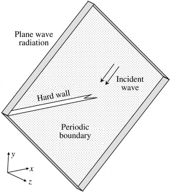
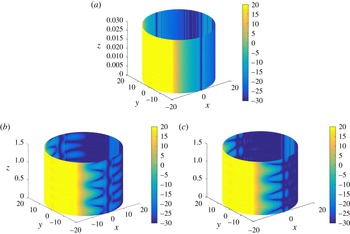
faces of the computational domain. The inlet boundary condition allows the introduction of the incident wave into the computation domain, which is intentionally designed in such a way (as in figure 3) to simplify the set-up of the incident wave and minimise any possible reflection from the computational domain. Furthermore, the plane wave radiation boundary condition is used to reduce possible sound wave reflections from the computational domain. Different refinement levels of the mesh have been tested to ensure a proper convergence of the simulation. The whole computation was performed on a desktop computer with an Intel core i7-4790 @
 $3.60~\text{GHz}$
processor and
 $24~\text{GB}$
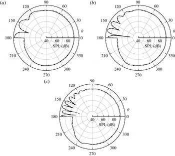
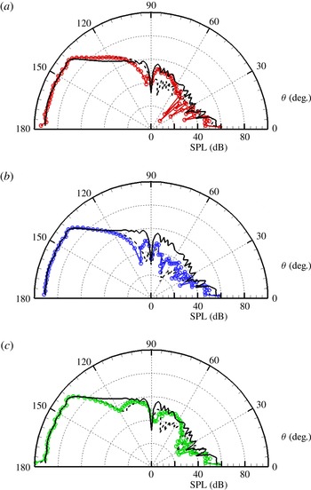
memory. The computational set-ups are first verified by using the 2D cases with a straight edge. The corresponding theoretical predictions are from the well-known 2D diffraction model (Noble Reference Noble1958; Wright Reference Wright2008). Figure 4 shows the sound pressure level (SPL,
 $20\log _{10}\overline{p(t)}/p_{0}$
, where
 $\overline{(\cdot )}$
is the time root mean square and
 $p_{0}=20~\unicode[STIX]{x03BC}\text{Pa}$
) results at a radial distance
 $r\triangleq \sqrt{x^{2}+y^{2}}=1~\text{m}$
with
 $f=500$
,
 $1000$
and
 $1500~\text{Hz}$
. It can be seen that the computational results and the theoretical predictions are almost identical, which verifies the computational set-up. For 3D computations of the cases with serrated edges, the maximum number of grid cells currently allowed on our desktop computer is approximately
 $2.5\times 10^{6}$
, which ensures a satisfactory points-per-wavelength value only for incident sound waves with frequencies
 $f<1000~\text{Hz}$
. The generalised minimal residual method (GMRES) solver with an iterative method is adopted and the corresponding computation time for each set-up is approximately
 $5000~\text{s}$
.
The computational domain and the boundary conditions used in the FEM commercial solver.

Comparisons of the SPL results for the total sound field at
 $r=1~\text{m}$
for the straight edge set-up. The results are from (– –) the numerical FEM solver and (–) the theoretical model (Noble Reference Noble1958; Wright Reference Wright2008) at (a)
 $500~\text{Hz}$
(
 $k=9.24$
), (b)
 $1000~\text{Hz}$
(
 $k=18.48$
) and (c)
 $1500~\text{Hz}$
(
 $k=27.72$
).

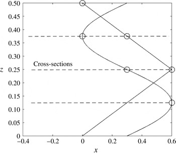
Two representative profiles
 $\unicode[STIX]{x1D712}(z)$
are considered in this work. One is sinusoidal-shaped and the other is sawtooth-shaped. The circles denote the three representative cross-sections passing through the tip, medial and root positions of the sinusoidal-shaped serrations.

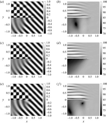
The near-field results from the theoretical model, where the serrations are sinusoidal-shaped with
 $\unicode[STIX]{x1D706}=0.5$
and
 $h_{s}=0.3$
. The incident wave of
 $f=1000~\text{Hz}$
is at
 $\unicode[STIX]{x1D703}=45^{\circ }$
. The instantaneous sound pressure (a,c,e) and the SPL results (b,d,f) are collected at (a,b) the tip cross-section, (c,d) the medial cross-section and (e,f) the root cross-section. The black straight line in each panel denotes the silhouette of the serrated flat plate at the corresponding cross-section.

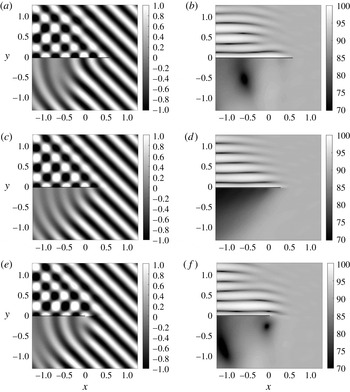
The near-field results from the theoretical model, where the serrations are sawtooth-shaped. Other set-ups are the same as those in figure 6.

Figure 5 shows the two representative serrations with either a sinusoidal- or a sawtooth-shaped profile in the numerical validations, for which various test conditions have been investigated and similar conclusions have been reached. For brevity, we primarily show numerical results for an incident wave of
 $1000~\text{Hz}$
at
 $\unicode[STIX]{x1D703}=45^{\circ }$
below. In this numerical set-up, the two profiles have
 $h_{s}/\unicode[STIX]{x1D706}=0.6$
and
 $\unicode[STIX]{x1D706}=0.5$
. In addition, the infinitely thin flat plate in the theoretical model has to be replaced by a very thin flat plate with a small thickness of
 $0.01$
in the numerical set-ups. Figure 5 also shows three cross-sections, where results from the theoretical model and the numerical solver will be extensively examined in the following. For simplicity, these three cross-sections will be referred to as the tip, medial and root cross-sections respectively.
First, to demonstrate the capability of the proposed theoretical model, figures 6 and 7 show the near-field results for the instantaneous sound pressure fields
 $p(t)$
and SPLs at the three representative
 $x$
–
 $y$
cross-sections. The SPL results in figure 6 clearly show that the serrated open ends affect the local sound pressure fields to some extent. In particular, the SPL results at the tip and root cross-sections are quite different from the SPL result at the medial cross-section, although the corresponding instantaneous sound pressure fields are still seemingly similar. The same observation can be made from the corresponding theoretical results for the sawtooth-shaped serrations (see figure 7).
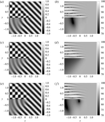
The near-field results from the commercial FEM solver. The serrations are sawtooth-shaped. Other set-ups are the same as those in figure 7.

The instantaneous pressure fields and the SPL fields in figures 6 and 7 are very similar, which suggests that the noise control performance of the sinusoidal- and sawtooth-shaped serrations is almost the same for the current geometrical set-ups at the frequency
 $f=1000~\text{Hz}$
. The following parametric study will show that the noise control performance becomes more different at higher frequencies (figure 13) and various dimensions (see figure 14). To ensure a satisfactory points-per-wavelength value, the current computation still adopts an incident sound wave frequency of
 $f=1000~\text{Hz}$
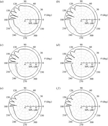
. To validate the proposed model, figure 8 shows the computational results from the FEM solver. The sawtooth-shaped serrations are used in the computation and other test set-ups are the same as those in figure 7. It can be seen that the theoretical predictions shown in figure 7 and the numerical results shown in figure 8 have almost identical patterns at the three representative cross-sections. The theoretical model, however, is quite efficient and can produce the above results in seconds.
Comparisons of the SPL results at
 $r=1$
, where (– –) denotes the results from the numerical solver and (–) denotes the theoretical predictions. (a,c,e) Results for the set-up with the sinusoidal-shaped serrations and (b,d,f) for sawtooth-shaped serrations, at (a,b) the tip cross-section, (c,d) the middle cross-section and (e,f) the root cross-section. Other set-ups are the same as those in figures 6 and 7.

To further quantitate the differences, figure 9 shows the SPL directivity patterns from the theoretical model and the FEM solver along the observation circle with
 $r\triangleq \sqrt{x^{2}+y^{2}}=1$
. The agreement between the two sets of results is quite good in most angular regions, with the largest difference of less than
 $1~\text{dB}$
in the angular region with
 $\unicode[STIX]{x1D703}$
between
 $180^{\circ }$
and
 $240^{\circ }$
in the tip and root cross-sections. However, the difference is relatively large (up to approximately
 $3~\text{dB}$
in the angular region close to
 $180^{\circ }$
) for the middle cross-section. We believe that two numerical issues cause the slight differences. First, the commercial software adopts an FEM solver that requires a large points-per-wavelength value to ensure satisfactory simulations of sound wave propagation and scattering. Second, for the convenience of generating computational meshes, the flat plat has a very small but finite thickness (set to 0.01) in the current numerical validation cases, which might affect the relatively weak scattered sound fields in the third quadrant. A better computer with more memory could easily address the above two issues.

3.2 Discussion
To further quantitate the noise control effects of the two representative types of serrations, figure 10 compares the so-called scattering cross-section that is usually used in the analysis of acoustic scattering. This specific criterion is defined as follows (Huang, Zhong & Liu Reference Huang, Zhong and Liu2014a ):
 $$\begin{eqnarray}\unicode[STIX]{x1D70E}(\unicode[STIX]{x1D703},z)=\lim _{r\rightarrow \infty }2\unicode[STIX]{x03C0}r\frac{\overline{p_{s}(r,\unicode[STIX]{x1D703},z)}^{2}}{\overline{p_{i}(r,\unicode[STIX]{x1D703},z)}^{2}}.\end{eqnarray}$$
In this work, we simply calculate the scattering cross-section by setting
 $r$
to a large value much greater than
 $\unicode[STIX]{x1D706}$
and
 $h_{s}$
. In addition, according to the second boundary condition, it is easy to see that the scattering cross-section is symmetrical with respect to the
 $x$
axis. Therefore, figure 10 only shows the scattering cross-section results in the angular region between
 $0^{\circ }$
and
 $180^{\circ }$
. As a comparison, the straight edge case is considered as well and the corresponding results are obtained by using the classical 2D rigid plate model (see figure 4) (Noble Reference Noble1958; Wright Reference Wright2008). The comparisons clearly show that both types of serrations are effective in reducing the scattering cross-sections compared with the straight edge set-up, especially in the angular region with
 $\unicode[STIX]{x1D703}$
between
 $0^{\circ }$
and
 $120^{\circ }$
. A maximum reduction of up to
 $10~\text{dB}$
is possible across the radiation angles in the same quadrant of the incident direction.

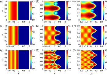
The SPL of the scattered sound field on the upper surface at
 $y=0^{+}$
, with (a,d,g) a straight edge, (b,e,h) sinusoidal-shaped serrations and (c,f,i) sawtooth-shaped serrations. (a,b,c) The results for an incident wave at
 $f=1000~\text{Hz}$
, (d,e,f) the results for
 $f=2000~\text{Hz}$
and (g,h,i) the results for
 $f=3000~\text{Hz}$
. The geometrical set-up of the serrations is shown in figure 5. Other set-ups are the same as those used in figures 6 and 7.

Figure 11 shows the scattering cross-sections for the whole far-field surface with
 $r\rightarrow \infty$
, which further confirms the abovementioned observation, i.e. both the sinusoidal- and sawtooth-shaped serrations can significantly reduce the scattering in the first and fourth quadrants.
The inherent noise control mechanisms might come from the periodic layouts of the serrations, which could possibly excite multiple scatterings in the lateral direction. Some of these scattering waves are prone to cancelling each other out and might collectively attenuate the total scattering cross-sections. On the other hand, the on-surface scattered SPL shown in figure 12 suggests an alternative noise control mechanism. For the current incident wave in the
 $x$
–
 $y$
domain, the straight edge produces no wave component in the
 $z$
direction (see figure 12
a,d,g). In contrast, the serrations excite some new wave components with non-zero wavenumbers in the
 $z$
direction. It can be seen that the sawtooth-shaped serrations (see figure 12
i) can excite waves with greater wavenumbers compared with the sinusoidal-shaped serrations (see figure 12
h). An ever-increasing wavenumber in the
 $z$
direction eventually results in an imaginary wavenumber in the
 $y$
direction. The corresponding wave does not propagate to the far-field region and, hence, the scattered sound waves are attenuated. Furthermore, by comparing figures 12(f) and 12(i), it can be seen that the serrations work more effectively for incident waves at higher frequencies. We also wish to point out that the scattered pressure field patterns in figures 12(b) and 12(c) are quite similar to the perturbed flow field pattern in a previous study using plasma actuators (figure 15 in Huang et al.
Reference Huang, Chan, Zhang and Gabriel2008a
). This close similarity suggests that it is possible to use active flow control actuators to obtain the same noise control performance from the current passive serrations.
Last but not least, we wish to point out that the theoretical prediction results given in figures 11 and 12 can be useful for verifying near-field and far-field experimental acoustic measurements.
3.3 Parametric studies
The overall computational cost for the theoretical model on a normal desktop computer with an Intel® Core i7 processor is significantly lower than the cost of the corresponding numerical validation cases run by the commercial finite element software. Specifically, our model is able to generate scattering cross-sections for various set-ups in seconds. In contrast, the same case set-up solved by the commercial finite element software with the unstructured meshes of
 $2.5\times 10^{6}$
gridpoints usually requires a few dozens of minutes. Overall, the proposed theoretical model is so efficient that we can use it to rapidly perform parametric studies. A couple of test cases are considered below to demonstrate this capability.
First, all of the above test cases were prepared for an incident wave at
 $\unicode[STIX]{x1D703}=45^{\circ }$
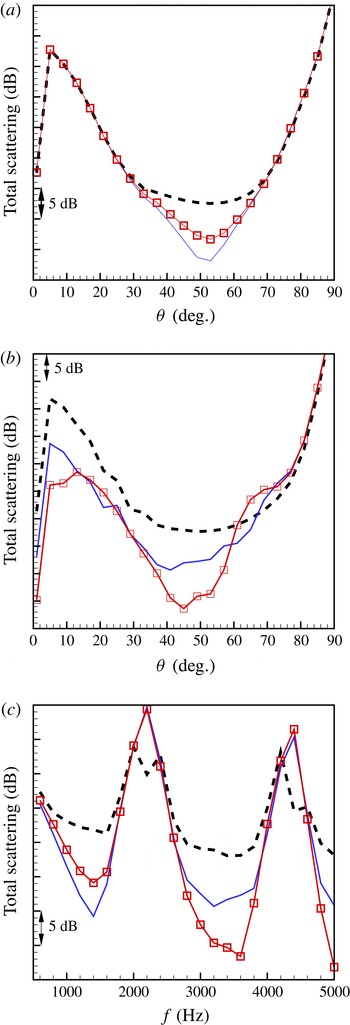
. Now, let us consider the possible noise control effect at different incident angles. Here, we modify the incident angle and examine the corresponding so-called total scattering cross-section:
 $$\begin{eqnarray}\unicode[STIX]{x1D70E}_{total}(\unicode[STIX]{x1D703})=\lim _{r\rightarrow \infty }2\unicode[STIX]{x03C0}r\frac{\displaystyle \int _{S}\overline{p_{s}(r,\unicode[STIX]{x1D703},z)}^{2}\,\text{d}S}{\displaystyle \int _{S}\overline{p_{i}(r,\unicode[STIX]{x1D703},z)}^{2}\,\text{d}S},\end{eqnarray}$$
where
 $S$
is the far-field surface of interest (e.g. the contour surface in figure 11). As shown in figures 10 and 11, the serrations mainly affect the scattering cross-sections in the radiation angular region between
 $0^{\circ }$
and
 $90^{\circ }$
. Hence, here we choose
 $S$
with the related
 $\unicode[STIX]{x1D703}\in [0,90]^{\circ }$
.
The total scattering cross-sections with respect to (a,b) different incident angles with (a)
 $f=1000~\text{Hz}$
and (b)
 $f=3500~\text{Hz}$
, and (c) a range of incident frequencies (with
 $\unicode[STIX]{x1D703}=45^{\circ }$
), (
 $--$
) with a straight edge, (–) with sinusoidal-shaped serrations and (
 $\Box$
) with sawtooth-shaped serrations. Other set-ups are the same as those used in figures 6 and 7.

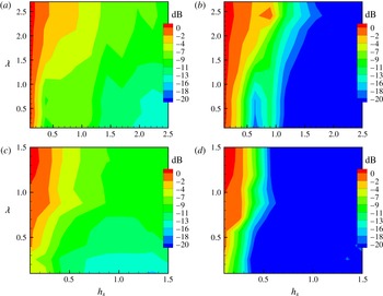
The contours of the total scattering cross-sections with respect to different geometrical values of
 $\unicode[STIX]{x1D706}$
and
 $h_{s}$
, (a,c) with sinusoidal-shaped serrations and (b,d) with sawtooth-shaped serrations. (a,b) Results at
 $f=1000~\text{Hz}$
and (c,d) results at
 $f=3500~\text{Hz}$
. Other set-ups are the same as those used in figures 6 and 7.

Figure 13(a) shows the theoretical variations of
 $\unicode[STIX]{x1D70E}_{total}(\unicode[STIX]{x1D703})$
with respect to
 $\unicode[STIX]{x1D703}$
, with all other parameters being the same as the previous test cases, i.e.
 $h_{s}=0.3,\unicode[STIX]{x1D706}=0.5,f=1000~\text{Hz}$
. It becomes immediately clear that the serrations, either sawtooth- or sinusoidal-shaped, are effective only for some incident waves with incident angles in between a certain range. In particular, for the current set-up, this effective range of incident angles is between
 $30^{\circ }$
and
 $72^{\circ }$
. The maximum reduction relative to the plate with no serrations is approximately
 $10~\text{dB}$
when
 $\unicode[STIX]{x1D703}$
is around
 $53^{\circ }$
. Another interesting finding from figure 13(a) is that the sinusoidal-shaped serrations slightly outperform the sawtooth-shaped serrations. This observation seems to contradict a previous work by Howe (Reference Howe1991b
), whose conclusion, however, was made for high-frequency cases. Hence, we study a new case at
 $f=3500~\text{Hz}$
in figure 13(b), which then shows the same conclusion as Howe’s work (Howe Reference Howe1991b
), i.e. sawtooth-shaped serrations generally perform better than sinusoidal-shaped serrations, and the noise control performance improves along with an increase in wave frequency. If we further examine figure 13(c), it becomes clear that sawtooth-shaped serrations are usually more effective than sinusoidal-shaped serrations when the incident frequency is higher than
 $1600~\text{Hz}$
. The corresponding wavelength is smaller than
 $h_{s}$
(currently 0.3), which suggests two points. First, a serration works more effectively when its characteristic length is larger than the wavelength of the incident wave. Second, it should be more appropriate to take the half root-to-tip distance
 $h_{s}$
than
 $\unicode[STIX]{x1D706}$
to be the characteristic length. In addition, figure 13(c) shows that for certain set-ups (e.g.
 $f\in [2000,2400]~\text{Hz}$
and
 $[4200,4600]~\text{Hz}$
with
 $\unicode[STIX]{x1D703}=45^{\circ }$
), instead of a noise reduction, the two serrations actually excite more noise scattering than that from a straight edge. Physically, the corresponding cases must contain constructive scattering waves instead of destructive cancellations.
Finally, we examine the total scattering cross-sections with respect to different possible values of the geometrical parameters
 $h_{s}$
and
 $\unicode[STIX]{x1D706}$
at
 $f=1000~\text{Hz}$
and
 $3500~\text{Hz}$
. The other parameters are the same as those in figures 6 and 7. This study can give the optimal geometrical design of the serrations at the given working conditions. Figure 14 shows the normalised results (by the maximum value of
 $\unicode[STIX]{x1D70E}_{total}(\unicode[STIX]{x1D703})$
from the cases with sinusoidal-shaped serrations), which are consistent with all of the abovementioned observations: (1) the sawtooth-shaped serrations are generally more effective in terms of the suppression of the scattering cross-sections, (2)
 $h_{s}$
is the key geometrical parameter and (3) the serrations are more effective when their characteristic length is larger than the wavelength of the incident waves.
4 Conclusion
In this paper, a theoretical model has been proposed for the study of sound scattering from a flat plate with leading-edge serrations, which act as a passive noise control device. The key achievement of this work is the analytic and rigorous description of the scattering from the lateral serrations by incorporating Fourier series expansions and the Wiener–Hopf method. The essential concept is to represent the laterally periodic serrations using Fourier series expansions and then model each decomposed component in an analytic way using the Wiener–Hopf method. The current work is solely focused on the study of a semi-infinite rigid flat plate with serrations of some representative set-ups. Nevertheless, the same concept that is behind this new theoretical model should also be applicable to the theoretical study of jet noise with chevrons (Carley Reference Carley2006; Tide & Srinivasan Reference Tide and Srinivasan2010).
Theoretically, the most critical part of the model is the definition of the half-plane Fourier transforms and the subsequent exercise to ensure the analytic and algebraic properties of the Wiener–Hopf kernel function. The resultant Wiener–Hopf kernel is a diagonal matrix and the related decomposition can be straightforwardly obtained. The proposed model has been demonstrated in some representative case studies with either sinusoidal- or sawtooth-shaped serrations, and the solutions have been compared favourably with the numerical results from a commercial finite element solver. Some important observations gained from the parametric studies are summarised here.
-
(1) Sawtooth-shaped serrations are more effective than sinusoidal-shaped serrations in terms of the suppression of scattering waves.
-
(2) In addition to the type of profile, a serration is mainly described using two geometrical parameters, the root-to-tip distance
$2h_{s}$
and the period
$\unicode[STIX]{x1D706}$
, and a bigger serration with larger
$\unicode[STIX]{x1D706}$
and
$h_{s}$
will reduce scattering waves more. -
(3) The final scattering cross-sections are more sensitive to
$h_{s}$
than
$\unicode[STIX]{x1D706}$
. -
(4) The serrations are more effective for incident waves at higher frequencies.


For serrations, the above findings also suggest that Mie scattering possibly predominates Rayleigh scattering. Nevertheless, the detailed mechanisms still call for further studies. Overall, the above conclusions are similar to those in the previous work by Howe (Reference Howe1991b ) because the problem set-up considered in the current work seems to be a system that is acoustically related to these previous wall turbulence scattering problems (Howe Reference Howe1991b ; Lyu et al. Reference Lyu, Azarpeyvand and Sinayoko2016) (more detailed discussion can be found in appendix B). For the latter problem set-up, we should appreciate the experimental efforts in the previous endeavours of Chong & Joseph (Reference Chong and Joseph2013) and Chong et al. (Reference Chong, Vathylakis, Joseph and Gruber2013). The current work, however, suggests a straightforward way to experimentally study and optimise the serration dimensions (Chong & Dubois Reference Chong and Dubois2016) simply from the perspective of acoustical scattering.
On the other hand, by showing the on-surface scattered waves, the current model suggests a new noise control mechanism due to serrations. In addition to forming multiple scattering to destructively cancel scattered waves, the current model shows that serrations excite some new modes in the lateral direction with such a large wavenumber that they eventually inhibit the wave propagation to far-field regions. Analogically, our work suggests that serrations might behave more like a convolution operator than a sonic crystal.
The whole work is mainly theoretical and the related development is complicated but rigorous. In particular, (2.15) is the most delicate part in the whole development which ensures the desired regularity property, and (2.24) and (2.25) should help to illuminate the noise control mechanisms of serrations from a mathematical perspective. Physically, the current model shows that serrations induce new periodical structures in the lateral direction, which may result in evanescent waves at the corresponding lateral modes. The possible noise generation mechanism due to turbulent structures and shear flows, however, was not considered in the current study. Overall, the concept behind the proposed model is highly innovative and should be able to significantly extend the current modelling capability of the Wiener–Hopf method. This work should be helpful in deepening the understanding of the inherent noise control mechanism of the silent flying capabilities of owls, and will provide a theoretical framework for analysing the design and optimisation of new low-noise aircraft and vehicles.
Acknowledgements
This work is partly supported by the National Science Foundation of China (grants 11322222 and 11561130148), a Newton Advanced Fellowship from the Royal Society (Ref. NA14081) and an Initiation Grant from the Hong Kong University of Science and Technology (No. IGN15EG07). The author is grateful to Mr B. Peng and Mr S. Zhong for preparing the numerical validations, Mr H. Jiang for some helpful discussions and Dr A. S. H. Lau for the proofreading of this paper. The author wishes to dedicate this paper to the memory of Geoffrey Lilley (1919–2015), who was the professor emeritus of aeronautics and astronautics at the University of Southampton and who guided the author to this interesting topic of stealthy flying owls (Lilley Reference Lilley1998, Reference Lilley2001) when the author had just started his PhD research in aeroacoustics 15 years ago at Southampton.
Appendix A. The serrated plate at zero angle of attack in a uniform flow
The proposed model studies the sound scattered when a sound wave is incident on an idealised aerofoil (a semi-infinite flat plate) with serrations in a stationary fluid medium. The same modelling technique can be simply extended to cases with a serrated plate at zero angle of attack in a uniform airflow by using the Prandtl–Glauert transformation. The required derivation is given here for the completeness of the current paper. For more details, the interested reader can refer to the literature (Huang et al. Reference Huang, Zhong and Stalnov2014b ).
For a flat plate at zero angle of attack in a uniform airflow (in the
 $x$
direction), the scattered sound field can be described by the convected wave equation
 $$\begin{eqnarray}\left(\frac{\unicode[STIX]{x2202}^{2}}{\unicode[STIX]{x2202}x^{2}}+\frac{\unicode[STIX]{x2202}^{2}}{\unicode[STIX]{x2202}y^{2}}+\frac{\unicode[STIX]{x2202}^{2}}{\unicode[STIX]{x2202}z^{2}}\right)\unicode[STIX]{x1D719}-\left(\frac{\unicode[STIX]{x2202}}{\unicode[STIX]{x2202}t}+M\frac{\unicode[STIX]{x2202}}{\unicode[STIX]{x2202}x}\right)^{2}\unicode[STIX]{x1D719}=0,\end{eqnarray}$$
where
 $M$
is the Mach number. First, we define
 $$\begin{eqnarray}x=\unicode[STIX]{x1D702}\tilde{x},\quad y={\tilde{y}},\quad z=\tilde{z},\quad \unicode[STIX]{x1D719}=\tilde{\unicode[STIX]{x1D719}}\text{e}^{-\text{i}kM\tilde{x}/\unicode[STIX]{x1D702}},\end{eqnarray}$$
where
 $\unicode[STIX]{x1D702}^{2}=1-M^{2}$
. Then, (A 1) can be simplified to
 $$\begin{eqnarray}\left(\frac{\unicode[STIX]{x2202}^{2}}{\unicode[STIX]{x2202}\tilde{x}^{2}}+\frac{\unicode[STIX]{x2202}^{2}}{\unicode[STIX]{x2202}{\tilde{y}}^{2}}+\frac{\unicode[STIX]{x2202}^{2}}{\unicode[STIX]{x2202}\tilde{z}^{2}}\right)\tilde{\unicode[STIX]{x1D719}}-\frac{1}{\unicode[STIX]{x1D702}^{2}}\frac{\unicode[STIX]{x2202}^{2}}{\unicode[STIX]{x2202}t^{2}}\tilde{\unicode[STIX]{x1D719}}=0.\end{eqnarray}$$
It can be seen that the coordinates and the incident waves are modified in the presence of a uniform mean flow. The subsequent derivation should be essentially the same from (2.5) onwards. Nevertheless, we should admit that the model developed in this paper does not take account of case set-ups with a shear flow (Dowling, Ffowcs Williams & Goldstein Reference Dowling, Ffowcs Williams and Goldstein1978).
Appendix B. The Wiener–Hopf model for a turbulent boundary pressure gust
Here, we briefly give the Wiener–Hopf model for the scattering of the pressure gust inside a turbulent boundary layer (TBL). This problem has been heavily studied and most previous works adopt Schwarzschild’s technique (Amiet Reference Amiet1975), which can be extended for problems with sawtooth-shaped serrations (Lyu et al. Reference Lyu, Azarpeyvand and Sinayoko2016). As shown in this paper, a model based on the Wiener–Hopf method can be extended to serrations with more complicated profiles by following the Fourier expansion approach. Hence, the Wiener–Hopf based model for a straight trailing edge is given below. It should be easy for the reader to further extend this model to take account of trailing-edge serrations by adopting the approach proposed in this paper.
Sketch of the problem with a turbulent pressure gust inside a boundary layer.

As shown in figure 15, the problem contains a rigid infinitely thin flat plat in the presence of a uniform flow with the Mach number
 $M_{0}$
in the positive
 $x$
direction (i.e. zero angle of attack). The attention of this problem is focused on the scattered sound pressure radiated from the trailing edge due to the interaction between the trailing edge and the pressure gust inside a boundary layer (such as Tollmien–Schlichting waves). This work also follows Amiet’s assumption of frozen turbulence (Amiet Reference Amiet1975), that is, the turbulent boundary layer remains unaffected by the trailing edge and is statically invariant as it convects past the trailing edge of the flat plate. The scattered sound field can be described by the convected wave equation
 $$\begin{eqnarray}\displaystyle \left(\frac{\unicode[STIX]{x2202}}{\unicode[STIX]{x2202}t}+M_{0}\frac{\unicode[STIX]{x2202}}{\unicode[STIX]{x2202}x}\right)^{2}\unicode[STIX]{x1D719}-\unicode[STIX]{x1D735}\unicode[STIX]{x1D719}=0. & & \displaystyle\end{eqnarray}$$
From the acoustic potential
 $\unicode[STIX]{x1D719}$
, we can obtain the scattered sound pressure
 $p_{s}$
, the particle velocity
 $\boldsymbol{v}=(u,v,w)$
and the acoustic density
 $\unicode[STIX]{x1D70C}$
by using the following relations:
 $$\begin{eqnarray}\displaystyle p_{s}=-\!\left(\frac{\unicode[STIX]{x2202}}{\unicode[STIX]{x2202}t}+M_{0}\frac{\unicode[STIX]{x2202}}{\unicode[STIX]{x2202}x}\right)\unicode[STIX]{x1D719},\quad \boldsymbol{v}=\unicode[STIX]{x1D735}\unicode[STIX]{x1D719},\quad \unicode[STIX]{x1D70C}=p_{s}. & & \displaystyle\end{eqnarray}$$
For simplicity, the common factor,
 $\exp (-\text{i}\unicode[STIX]{x1D714}t)$
, will be suppressed and only a two-dimensional geometrical set-up will be considered. The current problem is further subject to the following kinetic conditions:
 $$\begin{eqnarray}\displaystyle \left(\frac{\unicode[STIX]{x2202}}{\unicode[STIX]{x2202}t}+M_{0}\frac{\unicode[STIX]{x2202}}{\unicode[STIX]{x2202}x}\right)\unicode[STIX]{x1D709}(x)=\frac{\unicode[STIX]{x2202}\unicode[STIX]{x1D719}}{\unicode[STIX]{x2202}y}(x,0^{\pm }),\quad x>0, & & \displaystyle\end{eqnarray}$$
where
 $\unicode[STIX]{x1D709}$
is the normal particle displacement of a presumed sheet (at
 $y=0$
) that separates the upper (with
 $y\geqslant 0^{+}$
) and lower flows (with
 $y\leqslant 0^{-}$
), with
 $(\cdot )^{\pm }$
denoting the upper and lower positions respectively. Equation (B 3) relates the material derivative of the sheet layer to the normal acoustic velocity. Furthermore, for an inviscid fluid, the total pressure (i.e.
 $p_{s}+p_{g}$
) should be continuous across the sheet, resulting in
 $$\begin{eqnarray}p_{s}(x,0^{+})-p_{s}(x,0^{-})=\left(\frac{\unicode[STIX]{x2202}}{\unicode[STIX]{x2202}t}+M_{0}\frac{\unicode[STIX]{x2202}}{\unicode[STIX]{x2202}x}\right)\left(\unicode[STIX]{x1D719}(x,0^{+})-\unicode[STIX]{x1D719}(x,0^{-})\right)=A_{i}\text{e}^{\text{i}k_{x}x},\quad x>0,\end{eqnarray}$$
where the term on the right-hand side represents the wall gust pressure difference between the upper and lower walls were the trailing edge absent. With no loss of generality, here we simply consider a single mode with axial wavenumber at the tonal frequency
 $\unicode[STIX]{x1D714}$
, with
 $k_{x}=\unicode[STIX]{x1D714}/(0.7M_{0})$
and the related amplitude
 $A_{i}$
. It should be straightforward to study the scattering of a broadband turbulent gust through summations of different oblique wall pressure gust components with various wavenumbers and
 $\unicode[STIX]{x1D714}$
. In addition, the scattered field should satisfy the far-field radiation condition and the hard-wall condition, i.e.
 $$\begin{eqnarray}\displaystyle \left.\frac{\unicode[STIX]{x2202}\unicode[STIX]{x1D719}(x,y)}{\unicode[STIX]{x2202}y}\right|_{y=0}=0,\quad \forall x\leqslant 0. & & \displaystyle\end{eqnarray}$$
We define the conventional Fourier transform for the scattered sound fields as
 $$\begin{eqnarray}\displaystyle \unicode[STIX]{x1D6FD}(\unicode[STIX]{x1D6FC},y)\triangleq \int _{0}^{+\infty }p_{s}(x,y)\text{e}^{\text{i}\unicode[STIX]{x1D6FC}x}\,\text{d}x+\int _{-\infty }^{0}p_{s}(x,y)\text{e}^{\text{i}\unicode[STIX]{x1D6FC}x}\,\text{d}x=\unicode[STIX]{x1D6FD}_{+}(\unicode[STIX]{x1D6FC},y)+\unicode[STIX]{x1D6FD}_{-}(\unicode[STIX]{x1D6FC},y), & & \displaystyle\end{eqnarray}$$
where
 $\unicode[STIX]{x1D6FC}$
is the axial wavenumber. From (B 6), (B 1) can be transformed to
 $$\begin{eqnarray}\displaystyle \frac{\unicode[STIX]{x2202}^{2}\unicode[STIX]{x1D6FD}(\unicode[STIX]{x1D6FC},y)}{\unicode[STIX]{x2202}y^{2}}+\underbrace{\left[(\unicode[STIX]{x1D714}-M_{0}\unicode[STIX]{x1D6FC})^{2}-\unicode[STIX]{x1D6FC}^{2}\right]}_{\unicode[STIX]{x1D706}_{0}^{2}}\unicode[STIX]{x1D6FD}(\unicode[STIX]{x1D6FC},y)=0, & & \displaystyle\end{eqnarray}$$
which, by satisfying the radiation boundary condition, should produce solutions of the following generic form:
 $$\begin{eqnarray}\unicode[STIX]{x1D6FD}(\unicode[STIX]{x1D6FC},y)=\left\{\begin{array}{@{}ll@{}}A(\unicode[STIX]{x1D6FC})\text{e}^{\text{i}\unicode[STIX]{x1D706}_{0}y},\quad \quad & \forall y>0,\\ -A(\unicode[STIX]{x1D6FC})\text{e}^{-\text{i}\unicode[STIX]{x1D706}_{0}y},\quad \quad & \forall y<0.\end{array}\right.\end{eqnarray}$$
It is worthwhile to point out that (B 7) and (B 8) are different from the classical model for the rigid screen scattering problem (Wright Reference Wright2008). From the kinetic condition (B 3), we have
 $$\begin{eqnarray}A(\unicode[STIX]{x1D6FC})=-\frac{(\unicode[STIX]{x1D714}-M_{0}\unicode[STIX]{x1D6FC})\mathfrak{F}_{+}(\unicode[STIX]{x1D707})}{\unicode[STIX]{x1D706}_{0}},\quad \mathfrak{F}_{+}(\unicode[STIX]{x1D707})\triangleq \int _{0}^{+\infty }\unicode[STIX]{x1D709}(x)\text{e}^{\text{i}\unicode[STIX]{x1D6FC}x}\,\text{d}x.\end{eqnarray}$$
By applying the above Fourier transform to the scattered pressure difference,
 $p_{s}(x,0^{+})-p_{s}(x,0^{-})$
, and adopting equations (B 2) and the pressure continuity condition (B 4), we have
 $$\begin{eqnarray}\displaystyle \mathfrak{G}(\unicode[STIX]{x1D6FC}) & \triangleq & \displaystyle \int _{-\infty }^{+\infty }\left[\left(\frac{\unicode[STIX]{x2202}}{\unicode[STIX]{x2202}t}+M_{0}\frac{\unicode[STIX]{x2202}}{\unicode[STIX]{x2202}x}\right)\left(\unicode[STIX]{x1D719}(x,0^{+})-\unicode[STIX]{x1D719}(x,0^{-})\right)\right]\text{e}^{\text{i}\unicode[STIX]{x1D6FC}x}\,\text{d}x\nonumber\\ \displaystyle & = & \displaystyle -\text{i}(\unicode[STIX]{x1D714}-M_{0}\unicode[STIX]{x1D6FC})\left[\unicode[STIX]{x1D6FD}(\unicode[STIX]{x1D6FC},0^{+})-\unicode[STIX]{x1D6FD}(\unicode[STIX]{x1D6FC},0^{-})\right]=\mathfrak{G}_{+}(\unicode[STIX]{x1D6FC})+\mathfrak{G}_{-}(\unicode[STIX]{x1D6FC})\nonumber\\ \displaystyle & = & \displaystyle \int _{0}^{+\infty }A_{i}\text{e}^{\text{i}k_{x}x}\text{e}^{\text{i}\unicode[STIX]{x1D6FC}x}\,\text{d}x+\mathfrak{G}_{-}(\unicode[STIX]{x1D6FC})=-\frac{A_{i}}{\text{i}(\unicode[STIX]{x1D6FC}+k_{x})}+\mathfrak{G}_{-}(\unicode[STIX]{x1D6FC}),\end{eqnarray}$$
where
 $(\cdot )_{\pm }$
denote analytic on the upper and lower planes respectively. On substituting (2.13) and (B 9) into (B 10), we obtain the Wiener–Hopf equation for the current problem,
 $$\begin{eqnarray}\underbrace{\left[\text{i}\frac{(\unicode[STIX]{x1D714}-M_{0}\unicode[STIX]{x1D6FC})^{2}}{\unicode[STIX]{x1D706}_{0}}\right]}_{\mathfrak{K}(\unicode[STIX]{x1D6FC})}\mathfrak{F}_{+}(\unicode[STIX]{x1D6FC})=-\frac{A_{i}}{\text{i}(\unicode[STIX]{x1D6FC}+k_{x})}+\mathfrak{G}_{-}(\unicode[STIX]{x1D6FC}),\end{eqnarray}$$
where
 $\mathfrak{K}(\unicode[STIX]{x1D6FC})$
is the associated Wiener–Hopf kernel, which can be multiplicatively factorised to
 $\mathfrak{K}(\unicode[STIX]{x1D6FC})=\mathfrak{K}_{+}(\unicode[STIX]{x1D6FC})/\mathfrak{K}_{-}(\unicode[STIX]{x1D6FC})$
by using the well-known decomposition theorem in the classical monograph by Noble (Reference Noble1958) (p. 42), where
 $\mathfrak{K}_{+}(\unicode[STIX]{x1D6FC})$
and
 $\mathfrak{K}_{-}(\unicode[STIX]{x1D6FC})$
are analytic and bounded on the upper and lower complex planes respectively. Then, a closed-form solution is available by applying analytic continuation and Liouville’s theorem, yielding
 $$\begin{eqnarray}\mathfrak{F}_{+}(\unicode[STIX]{x1D6FC})=-\frac{A_{i}}{\text{i}(\unicode[STIX]{x1D6FC}+k_{x})}\frac{\mathfrak{K}_{-}(\unicode[STIX]{x1D6FC}^{\ast })}{\mathfrak{K}_{+}(\unicode[STIX]{x1D6FC})},\end{eqnarray}$$
where
 $\unicode[STIX]{x1D6FC}^{\ast }$
is the pole of (B 11), i.e.
 $\unicode[STIX]{x1D6FC}^{\ast }=-k_{x}$
. By substituting the above solution of
 $\mathfrak{F}_{+}(\unicode[STIX]{x1D707})$
into (B 8) and (B 9), we are able to obtain the Fourier transformed scattered field,
 $\unicode[STIX]{x1D6FD}(\unicode[STIX]{x1D6FC},y)$
, which leads to the solution of the scattered field by applying an inverse Fourier transform. The derivation and the related discussion of the above solution are essentially the same as those between (2.34) and (2.41) in the main text and, thus, are omitted here for brevity.
After comparing the Wiener–Hopf equations (2.38) and (B 11), it should be straightforward to extend the current TBL scattering model to further take account of serrations. Furthermore, the related noise attenuation mechanisms should be similar to those discussed in the main text of this paper. Hence, the two problems are regarded as acoustically similar in this work.
Appendix C. The Wiener–Hopf model for oncoming flows with a gust velocity component
Up to now, the current paper had been primarily focused on the scattering of incident sound pressure waves (see figure 16). In this section, we consider the scattering of a horizontal uniform mean flow that carries a gust velocity component in the
 $y$
direction. This is a classical benchmark problem in aeroacoustics (ICASE category 6) and has been heavily studied mainly by Schwarzschild’s technique (Roger & Moreau Reference Roger and Moreau2005). Instead, here we give the main steps leading to the associated Wiener–Hopf model.
Sketch of the problem with a gust velocity component in the
 $y$
direction.

The scattered sound field can be described by the governing equation (B 1), which can be further simplified to the classical wave equation (A 3) using the Prandtl–Glauert transformation. For simplicity, we only consider a two-dimensional set-up and suppress the common factor
 $\exp (-\text{i}\unicode[STIX]{x1D714}t)$
. Then, the acoustical potential
 $\tilde{\unicode[STIX]{x1D713}}_{s}$
in the transformed domain should satisfy the Helmholtz equation:
 $$\begin{eqnarray}\left(\frac{\unicode[STIX]{x2202}^{2}}{\unicode[STIX]{x2202}\tilde{x}^{2}}+\frac{\unicode[STIX]{x2202}^{2}}{\unicode[STIX]{x2202}{\tilde{y}}^{2}}\right)\tilde{\unicode[STIX]{x1D713}}_{s}+\tilde{k}^{2}\tilde{\unicode[STIX]{x1D713}}_{s}=0.\end{eqnarray}$$
The gust velocity component is
 $v_{g}(\tilde{x},{\tilde{y}})=A_{g}\exp (\text{i}\tilde{k_{x}}\tilde{x})$
. Further, the current problem will satisfy the following conditions:
 $$\begin{eqnarray}\displaystyle & \displaystyle \left.\frac{\unicode[STIX]{x2202}\unicode[STIX]{x1D713}_{s}}{\unicode[STIX]{x2202}{\tilde{y}}}\right|_{y=0}=-A_{g}\exp (\text{i}\tilde{k_{x}}\tilde{x}),\quad \tilde{x}<0, & \displaystyle\end{eqnarray}$$
 $$\begin{eqnarray}\displaystyle & \displaystyle \unicode[STIX]{x1D713}_{s}|_{{\tilde{y}}=0}=0,\quad \tilde{x}>0, & \displaystyle\end{eqnarray}$$
where (C 2) is the hard-wall boundary condition and (C 3) is valid since
 $\tilde{\unicode[STIX]{x1D713}_{s}}$
is an odd function. Immediately, it can be seen that the above boundary conditions are similar to (2.6) and (2.7) for the problem described in the main text, or similar to (B 4) and (B 5) for the problem described in appendix B. Then, all of the following derivations based on the Wiener–Hopf method should essentially follow the same steps as those between (B 6) and (B 12) and, therefore, are omitted below for brevity.
Finally, it is worthwhile to emphasise again that Schwarzschild’s technique can be directly applied to solve (C 1)–(C 3) (Lyu et al. Reference Lyu, Azarpeyvand and Sinayoko2016), while the Wiener–Hopf method can offer a mathematically rigorous model, which can be further extended to set-ups of leading- and trailing-edge serrations of various shapes by using the Fourier expansion approach proposed in this paper.