1 Introduction
The regenerative cooling system in most liquid rocket engines operates at a high-pressure condition above the critical pressure (e.g. the critical pressure for parahydrogen that is a typical propellant for liquid rocket engines is
 $p_{c}=1.28377$
MPa) and also at a high Reynolds number condition. Because of these extreme flow conditions, the propellant fluid in the regenerative cooling system becomes a supercritical fluid and the developing boundary layer along the cooling channel is in a fully developed turbulent state. Therefore, understandings of the turbulence statistics in turbulent boundary layers at supercritical pressure (i.e. supercritical turbulent boundary layers) and their underlying flow physics are crucial for developing a reliable liquid rocket engine. In addition to the liquid rocket engine application, as mentioned in the review paper by Yoo (Reference Yoo2013), supercritical fluids have been used in many industrial applications, such as supercritical steam generators in power plants, refrigerating systems with supercritical
 $\text{CO}_{2}$
, supercritical fluids for concentrated solar power plants, etc. In such applications, physical understandings of the supercritical turbulent boundary layers are also essential.
The well-known peculiar behaviour of supercritical fluids occurs within a narrow temperature range through the pseudo-critical temperature
 $T_{pc}$
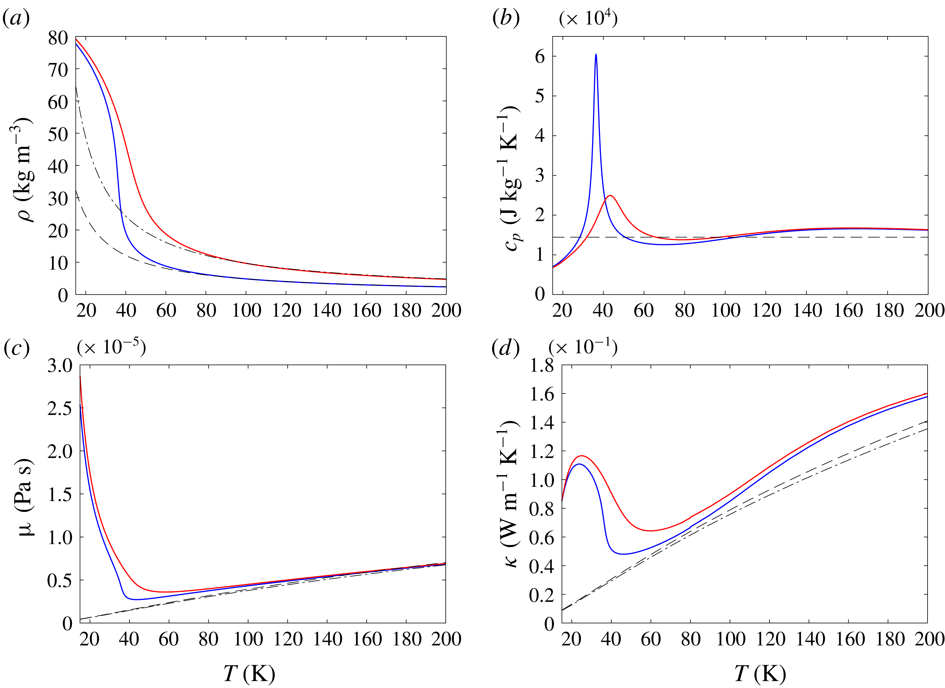
. Figure 1 shows the temperature dependency of density, specific heat at constant pressure
 $c_{p}$
, shear viscosity
 $\unicode[STIX]{x1D707}$
and thermal conductivity
 $\unicode[STIX]{x1D705}$
for parahydrogen at two different supercritical pressure conditions
 $p=2$
and 4 MPa. The thermodynamic properties under the perfect-gas relations and the fluid transport properties using Sutherland’s law are also plotted in the figure. When the fluid temperature varies through
 $T_{pc}$
, pseudo-boiling phenomena occur and a supercritical fluid behaves as a liquid-like high-density fluid when
 $T<T_{pc}$
and a gas-like low-density fluid at
 $T>T_{pc}$
. Also, the specific heat at constant pressure
 $c_{p}$
reaches its maximum value at
 $T=T_{pc}$
at a given supercritical pressure condition. The transition of the thermodynamic and fluid transport properties from a liquid-like fluid to a gas-like fluid through
 $T_{pc}$
occurs continuously at supercritical pressure, although the fluid properties vary abruptly within a narrow temperature range. We call this transitional state (i.e. the pseudo-boiling process) the ‘transcritical condition’. Also, we define the transcritical turbulent boundary layer to be the turbulent boundary layer at supercritical pressure, where the transcritical condition exists within the boundary layer. Within the transcritical condition, the thermodynamic properties significantly deviate from those of a perfect fluid due to the strongly nonlinear real-fluid effects. Here we use the ‘real-fluid effects’ to describe the deviations of the thermodynamic and fluid transport properties from the perfect fluid assumption. The real-fluid effects in supercritical fluids are especially noticeable at the transcritical condition and lower-temperature range (
 $T<T_{pc}$
) where the thermodynamic and fluid transport properties vary abruptly and significantly deviate from the perfect-gas relations and Sutherland’s law. By increasing the fluid temperature from
 $T<T_{pc}$
toward the transcritical condition, the density, shear viscosity and thermal conductivity (and also speed of sound although not shown) decrease while the specific heat at constant pressure
 $c_{p}$
(and also specific heat
 $\unicode[STIX]{x1D6FE}$
) increases and shows a peak at
 $T=T_{pc}$
. As shown in figure 1, these abrupt variations in fluid properties become more severe if the pressure approaches the critical pressure (i.e. the higher-pressure condition
 $p=4$
MPa shows more gentle variations than the lower-pressure condition
 $p=2$
MPa).
Variable thermodynamic and fluid transport properties for parahydrogen using REFPROP (NIST Standard Reference Database 23, Version 9.0): (a) density, (b) specific heat at constant pressure, (c) shear viscosity, (d) thermal conductivity. Blue,
 $p=2.0$
MPa; red,
 $p=4.0$
MPa; thin black dashed and dashed-dotted lines, the perfect-gas relations and Sutherland’s law (
 $\unicode[STIX]{x1D70C}=p/(RT)$
,
 $c_{p}=\unicode[STIX]{x1D6FE}R/(\unicode[STIX]{x1D6FE}-1)$
with the constant heat capacity ratio
 $\unicode[STIX]{x1D6FE}=1.4$
,
 $\unicode[STIX]{x1D707}=\unicode[STIX]{x1D707}_{273.16K}(273.16+C)/(T+C)(T/273.16)^{3/2}$
where
 $C=72$
, and
 $\unicode[STIX]{x1D705}=\unicode[STIX]{x1D707}c_{p}/Pr$
where we use the Prandtl number
 $Pr=0.72$
) at
 $p=2$
and 4 MPa.

Regarding the impact of the severe real-fluid effects at the transcritical condition on near-wall turbulence, experimental data show a significant change in mean wall statistics when the wall temperature approaches
 $T_{pc}$
(e.g. Yamagata et al. (Reference Yamagata, Nishikawa, Hasegawa, Fujii and Yoshida1972), more details may be found in the review paper by Yoo (Reference Yoo2013)). Yoo (Reference Yoo2013) mentioned that when the wall temperature varies through the pseudo-critical temperature
 $T_{pc}$
, both molecular and turbulence transfers can be strongly affected by the abrupt variations in thermodynamic and fluid transport properties at the transcritical condition. Yoo (Reference Yoo2013) also stated that the variation in density can especially affect turbulence production by virtue of the flow acceleration due to the thermal expansion of the heated fluid. However, it should be noted that, since it is extremely difficult to measure turbulence statistics (even mean velocity and temperature profiles) accurately in experiments at such an extreme high-pressure condition, there is little turbulence statistics available for turbulent boundary layers at supercritical pressure conditions. Because of the difficulty in measuring the flow quantities in experiments, the turbulence statistics and their underlying flow physics behind the peculiar behaviour of the supercritical turbulent boundary layers at the transcritical condition are far from being fully understood. To understand the turbulent boundary layers at the transcritical conditions and also to develop a reliable turbulence model to predict the turbulent boundary layer characteristics, it is crucial that we first need to understand the detailed turbulence statistics and their underlying flow physics in the transcritical turbulent boundary layers.
Considering the difficulty in experiments, numerical simulation is an attractive choice to understand the detailed flow physics involved in the transcritical turbulent boundary layers. Most of the existing numerical simulations for the transcritical turbulent boundary layers use Reynolds-averaged Navier–Stokes (RANS) models (e.g. Bellmore & Reid Reference Bellmore and Reid1983; Cheng, Kuang & Yang Reference Cheng, Kuang and Yang2007; Yang et al. Reference Yang, Oka, Ishiwatari, Liu and Yoo2007; He, Kim & Bae Reference He, Kim and Bae2008, see more complete list in Yoo Reference Yoo2013), and thus focus on ensemble-mean flow quantities. However, the RANS simulations show scattered results depending on the employed RANS model (Yoo Reference Yoo2013). Because of the lack of reliable turbulence statistics, a critical issue here is that it is difficult to judge that which model is better suited and also it is difficult to develop a better model by incorporating the flow physics in the transcritical boundary layers. Also, although a constant turbulent Prandtl number is typically used in the RANS simulations, it is not obvious that the turbulent Prandtl number is constant across the boundary layer where the thermodynamic and fluid transport properties vary abruptly within the transcritical boundary layers.
A straightforward approach to investigating the flow physics and the resultant detailed turbulence statistics in transcritical turbulent boundary layers is to conduct direct numerical simulation (DNS). DNS is an attractive choice for mainly two reasons: DNS can (i) provide detailed turbulence statistics and the underlying flow physics which are difficult to obtain experimentally; and (ii) directly analyse the interactions between near-wall turbulence and the pseudo-boiling process (i.e. variable thermodynamic and fluid transport properties at the transcritical condition).
Although DNS is one of the most promising approaches to elucidate the physics of the transcritical turbulent boundary layers, there are very limited DNS (and also large-eddy simulation (LES)) studies to investigate the transcritical turbulent boundary layers (to our knowledge, there is no DNS study of the canonical flat-plate transcritical turbulent boundary layer). This is primarily because an accurate and robust numerical simulation of the transcritical flows becomes extremely difficult under the abrupt variations in thermodynamic properties at the transcritical condition. Simply put, spurious grid-to-grid pressure oscillations arise when the steep variation in thermodynamic properties is numerically captured in a conservative form of the compressible flow governing equations. The spurious pressure oscillations remain as grid-to-grid oscillations even if the mesh is refined, while the physical pressure fluctuations have finite length scales. This issue has been extensively discussed in compressible multicomponent flows (e.g. Abgrall Reference Abgrall1996; Karni Reference Karni1996; Shyue Reference Shyue1998; Abgrall & Karni Reference Abgrall and Karni2001; Johnsen & Colonius Reference Johnsen and Colonius2006), and also in supercritical flows at the transcritical condition by Terashima & Koshi (Reference Terashima and Koshi2012), Hickey et al. (Reference Hickey, Ma, Ihme and Thakur2013), Kawai, Terashima & Negishi (Reference Kawai, Terashima and Negishi2015). These spurious pressure oscillations incur a numerical stability problem and also induce non-physical breakdown of the near-wall streak structures in the transcritical turbulent boundary layer, as shown in Kawai et al. (Reference Kawai, Terashima and Negishi2015). Because of this numerical issue, conducting DNS (and also LES) of supercritical flows at the transcritical condition is not straightforward, especially when the pressure condition is close to the critical pressure
 $p_{c}$
at which the variations in thermodynamic properties get steeper, as shown in figure 1.
Although solving the full compressible Navier–Stokes equations incurs the numerical stability issue at the transcritical condition, by employing the low Mach number assumption of the compressible Navier–Stokes equations (i.e. neglecting the acoustic interactions and compressibility effects) one can avoid this numerical difficulty. By solving the compressible mass, momentum and enthalpy equations under the low Mach number assumption, and also neglecting the viscous dissipation term in the energy equation, Bae, Yoo & Choi (Reference Bae, Yoo and Choi2005), Bae, Yoo & McEligot (Reference Bae, Yoo and Mceligot2008) conducted DNS to study heated
 $\text{CO}_{2}$
transcritical turbulent vertical pipe and annular flows with buoyancy effects. Although relatively coarse grid resolution (streamwise and radial resolutions in wall units of
 $\unicode[STIX]{x0394}x^{+}\approx 14.55$
and
 $(R\unicode[STIX]{x0394}\unicode[STIX]{x1D703})^{+}\approx 9.14$
) with a second-order accurate numerical method was employed, the detailed mean flow quantities and turbulence statistics including Reynolds stresses were provided from their DNS. They found that the ejection and sweep motions of near-wall turbulence become weakened by stabilizing effects from the variable fluid properties and buoyancy effects. More recently, Nemati et al. (Reference Nemati, Patel, Boersma and Pecnik2015, Reference Nemati, Patel, Boersma and Pecnik2016) and Peeters et al. (Reference Peeters, Pecnik, van der Hagen and Boersma2016) also used DNS by solving the same set of equations (i.e. the mass, momentum and enthalpy equations) with the low Mach number assumption of the compressible Navier–Stokes equations to study heated and cooled
 $\text{CO}_{2}$
transcritical turbulent pipe and annular flows. The transcritical flows show large thermodynamic property variations, and the detailed turbulence statistics, turbulent kinetic energy budget and turbulent structures that are altered by the property variations were investigated. Although there are extensive DNS studies of turbulent shear layers with mixing of supercritical fluids by solving the full compressible Navier–Stokes equations (Miller & Bellan Reference Miller and Bellan1999; Miller, Harstad & Bellan Reference Miller, Harstad and Bellan2001; Okong’o & Bellan Reference Okong’o and Bellan2002; Masi et al.
Reference Masi, Bellan, Harstad and Okong’o2013), for transcritical turbulent boundary layer flows, the existing DNS studies employ the low Mach number assumption of the compressible Navier–Stokes equations.
In this study, we use DNS and solve the full compressible Navier–Stokes equations without the low Mach number assumption to investigate nominally zero-pressure-gradient flat-plate turbulent boundary layers with heated and unheated isothermal walls at supercritical pressures. The motivation of this study is to elucidate the flow physics such as the interactions between the near-wall turbulence and peculiar abrupt variations in thermodynamic and fluid transport properties at the transcritical condition and also to provide detailed turbulence statistics in the canonical flat-plate turbulent boundary layer at supercritical pressures. By directly solving the full compressible Navier–Stokes equations, we may also provide evaluation data for the low Mach number assumption that is widely used in prior studies (Bae et al. Reference Bae, Yoo and Choi2005, Reference Bae, Yoo and Mceligot2008; Nemati et al. Reference Nemati, Patel, Boersma and Pecnik2015, Reference Nemati, Patel, Boersma and Pecnik2016; Peeters et al. Reference Peeters, Pecnik, van der Hagen and Boersma2016).
This paper is organized as follows. The governing equations, numerical methods, simulation parameters and verification of the quality of the present DNS data are described in § 2. In the present study, low-temperature (below the pseudo-critical temperature
 $T_{\infty }<T_{pc}$
) parahydrogen fluid at supercritical pressures is heated by the high-temperature isothermal wall (above
 $T_{pc}$
, i.e.
 $T_{w}>T_{pc}$
), and thus the developed heated transcritical turbulent boundary layers may be studied, where the flow temperature varies through the pseudo-critical temperature
 $T_{pc}$
within the boundary layers. In § 3, we first discuss the turbulence statistics to investigate the influence of the peculiar behaviour of variable thermodynamic and fluid transport properties at the transcritical condition on the turbulent boundary layers. Then, the mechanisms of the obtained turbulence statistics are discussed with visualizations of instantaneous flow fields in § 4.
2 Numerical methodology and verification
2.1 Governing equations and numerical methods
In this study, we directly solve the full compressible Navier–Stokes equations. However, there is a numerical stability issue when solving the compressible Navier–Stokes equations at the transcritical condition. When numerically capturing the abrupt variation in fluid properties at the transcritical condition (see figure 1), a straightforward approach of numerically solving the compressible Navier–Stokes equations for the mass, momentum and total energy induces non-physical spurious pressure oscillations. Similar spurious pressure oscillations are known to be generated when numerically capturing material interfaces in compressible multicomponent flow simulations (e.g. Abgrall Reference Abgrall1996; Karni Reference Karni1996). As shown in Kawai et al. (Reference Kawai, Terashima and Negishi2015), the non-physical oscillations incur a numerical stability issue and also induce non-physical breakdown of the near-wall streak structures. To avoid the spurious oscillations for stable and accurate turbulent flow computation at the transcritical condition, the method of Kawai et al. (Reference Kawai, Terashima and Negishi2015) is used in this study.
The employed governing equations are the full compressible Navier–Stokes equations for the mass, momentum and pressure evolution
 $$\begin{eqnarray}\displaystyle & \displaystyle \frac{\unicode[STIX]{x2202}\unicode[STIX]{x1D70C}}{\unicode[STIX]{x2202}t}+\unicode[STIX]{x1D735}\boldsymbol{\cdot }(\unicode[STIX]{x1D70C}\boldsymbol{u})=0, & \displaystyle\end{eqnarray}$$
 $$\begin{eqnarray}\displaystyle & \displaystyle \frac{\unicode[STIX]{x2202}\unicode[STIX]{x1D70C}\boldsymbol{u}}{\unicode[STIX]{x2202}t}+\unicode[STIX]{x1D735}\boldsymbol{\cdot }(\unicode[STIX]{x1D70C}\boldsymbol{u}\otimes \boldsymbol{u}+p\text{}\underline{\unicode[STIX]{x1D739}}-\text{}\underline{\unicode[STIX]{x1D749}})=0, & \displaystyle\end{eqnarray}$$
 $$\begin{eqnarray}\displaystyle & \displaystyle \frac{\unicode[STIX]{x2202}p}{\unicode[STIX]{x2202}t}+\boldsymbol{u}\boldsymbol{\cdot }\unicode[STIX]{x1D735}p+\unicode[STIX]{x1D70C}c_{s}^{2}\unicode[STIX]{x1D735}\boldsymbol{\cdot }\boldsymbol{u}-\frac{1}{\unicode[STIX]{x1D70C}}\frac{\unicode[STIX]{x1D6FC}_{p}}{c_{v}\unicode[STIX]{x1D6FD}_{t}}\left(\text{}\underline{\unicode[STIX]{x1D749}}\boldsymbol{ : }\text{}\underline{\boldsymbol{S}}-\unicode[STIX]{x1D735}\boldsymbol{\cdot }\boldsymbol{q}\right)=0, & \displaystyle\end{eqnarray}$$
where
 $\unicode[STIX]{x1D70C}$
is the density,
 $\boldsymbol{u}$
is the velocity vector,
 $p$
is the static pressure,
 $\text{}\underline{\unicode[STIX]{x1D739}}$
is the unit tensor,
 $c_{s}=\sqrt{(\unicode[STIX]{x2202}p/\unicode[STIX]{x2202}\unicode[STIX]{x1D70C})_{e}+(p/\unicode[STIX]{x1D70C}^{2})(\unicode[STIX]{x2202}p/\unicode[STIX]{x2202}e)_{\unicode[STIX]{x1D70C}}}$
is the speed of sound,
 $c_{v}=(\unicode[STIX]{x2202}e/\unicode[STIX]{x2202}T)_{V}$
is the specific heat at constant volume,
 $\unicode[STIX]{x1D6FC}_{p}=(1/V)(\unicode[STIX]{x2202}V/\unicode[STIX]{x2202}T)_{p}$
is the thermal expansion coefficient,
 $\unicode[STIX]{x1D6FD}_{t}=-(1/V)(\unicode[STIX]{x2202}V/\unicode[STIX]{x2202}p)_{T}$
is the isothermal compressibility coefficient,
 $\boldsymbol{q}=-\unicode[STIX]{x1D705}\unicode[STIX]{x1D735}T$
is the heat flux vector,
 $\unicode[STIX]{x1D705}$
is the thermal conductivity,
 $T$
is the temperature and
 $:$
is the inner product of tensors. The viscous stress tensor is
 $\text{}\underline{\unicode[STIX]{x1D749}}=\unicode[STIX]{x1D707}(2\text{}\underline{\boldsymbol{S}})-(2/3)\unicode[STIX]{x1D707}(\unicode[STIX]{x1D735}\boldsymbol{\cdot }\boldsymbol{u})\text{}\underline{\unicode[STIX]{x1D739}}$
, where
 $\unicode[STIX]{x1D707}$
is the shear viscosity, and
 $\text{}\underline{\boldsymbol{S}}$
is the strain rate tensor
 $\text{}\underline{\boldsymbol{S}}=(1/2)(\unicode[STIX]{x1D735}\boldsymbol{u}+(\unicode[STIX]{x1D735}\boldsymbol{u})^{\text{T}})$
. Since the pressure evolution equation (2.3) can be derived from the mass, momentum and total energy equations, solving the pressure evolution equation is mathematically equivalent to solving the total energy equation. Detailed derivations of the pressure evolution equation (2.3) for the compressible Navier–Stokes equations may be found in Kawai et al. (Reference Kawai, Terashima and Negishi2015). In this study, the buoyancy term is not considered in order to study the strong effects of variable properties at the transcritical condition without the buoyancy effect.
The variable thermodynamic and fluid transport properties in the governing equations (i.e.
 $T$
,
 $c_{v}$
,
 $c_{s}$
,
 $\unicode[STIX]{x1D6FC}_{p}$
,
 $\unicode[STIX]{x1D6FD}_{t}$
,
 $\unicode[STIX]{x1D707}$
and
 $\unicode[STIX]{x1D705}$
) are evaluated by the tabulated look-up table method based on the NIST reference thermodynamic and fluid transport properties database (NIST Standard Reference Database 23, Version 9.0). In this approach, using the NIST database we first tabulate the thermodynamic and fluid transport quantities in the density and pressure parameter space at a preset constant interval, and then use the tabulated look-up database to evaluate the quantities in the simulation. In this study, the look-up table consists of
 $2001\times 2001$
data points in the density and pressure parameter space (with a constant interval of
 $\unicode[STIX]{x0394}\unicode[STIX]{x1D70C}\approx 0.039~\text{kg}~\text{m}^{-3}$
and
 $\unicode[STIX]{x0394}p\approx 0.0013~\text{MPa}$
), and the quantities are interpolated with a linear interpolation. The present approach provides a sufficiently accurate evaluation of the thermodynamic and fluid transport properties throughout the transcritical condition, whereas existing widely used equation of state and fluid transport models such as the models of Soave–Redlich–Kwong (Soave Reference Soave1972) type or Peng & Robinson (Reference Peng and Robinson1976) type for the equation of state and the Ely & Hanley (Reference Ely and Hanley1981) and Chung et al. (Reference Chung, Ajlan, Lee and Starling1988) transport coefficient models fail to predict the abrupt variations at the transcritical condition (Kawai et al.
Reference Kawai, Terashima and Negishi2015).
The present study directly solves the pressure-based full compressible Navier–Stokes equations (2.1)–(2.3) using DNS. The spatial derivatives are evaluated by a tridiagonal sixth-order compact difference scheme (Lele Reference Lele1992). The compact difference scheme is a non-dissipative method with low dispersion errors, and thus is suitable for resolving the broadband scales of turbulence. An eighth-order low-pass filter (Lele Reference Lele1992; Gaitonde & Visbal Reference Gaitonde and Visbal2000) is applied to
 $\unicode[STIX]{x1D70C}$
,
 $\unicode[STIX]{x1D70C}\boldsymbol{u}$
and
 $p$
, where the filter parameter
 $\unicode[STIX]{x1D6FC}_{f}$
is fixed at 0.495. This parameter needs to satisfy
 $-0.5<\unicode[STIX]{x1D6FC}_{f}\leqslant 0.5$
, and a higher value of
 $\unicode[STIX]{x1D6FC}_{f}$
indicates a less dissipative filter (the dissipation is biased toward shorter waves). Our prior numerical experiences (Kawai & Fujii Reference Kawai and Fujii2008; Kawai & Lele Reference Kawai and Lele2010) suggest the appropriateness of applying
 $\unicode[STIX]{x1D6FC}_{f}=0.495$
for high-fidelity turbulent flow computations. The artificial mass diffusivity (Kawai et al.
Reference Kawai, Terashima and Negishi2015) is introduced to the mass and momentum equations where it is necessary to capture the abrupt density variations at the transcritical condition numerically, while maintaining a system free from spurious oscillation. The artificial mass diffusivity is localized in the regions of under-resolved sharp variation in density, automatically switching-off where the flow is well resolved. As will be shown in § 2.3, the present sufficient grid resolution for DNS and the grid-converged turbulence statistics verify that the dissipation introduced by the artificial mass diffusivity is minimal compared to the physical terms and does not affect the results discussed in the paper. The explicit third-order total variation diminishing Runge–Kutta scheme by Shu & Osher (Reference Shu and Osher1988) is used for time integration. The non-dimensionalized time-step size used in the present DNS is
 $\unicode[STIX]{x0394}t\cdot u_{\infty }/\unicode[STIX]{x1D6FF}_{0}=1.2\times 10^{-4}$
where
 $u_{\infty }$
is the free-stream velocity and
 $\unicode[STIX]{x1D6FF}_{0}$
is approximately 99 % of the boundary layer thickness at the inlet of the heated computational domain (i.e. left inlet boundary of the right heated computational domain in figure 2), and the corresponding maximum inviscid Courant–Friedrichs–Lewy number is approximately 0.7. The detailed discussions on the capability of the present governing equations and the numerical methods may be found in Kawai et al. (Reference Kawai, Terashima and Negishi2015).
2.2 Case set-up
The present study considers nominally zero-pressure-gradient heated transcritical and unheated non-transcritical fully developed parahydrogen turbulent boundary layers on a flat plate at two different supercritical pressure conditions,
 $p=2$
and 4 MPa (where
 $p_{c}=1.28377$
MPa for parahydrogen). The unheated non-transcritical turbulent boundary layers considered in this study are low temperature (
 $T_{\infty }=25$
K) fully developed turbulent boundary layers with an unheated isothermal wall condition
 $T_{w}=T_{\infty }$
. For the heated transcritical turbulent boundary layers, the unheated non-transcritical turbulent boundary layer is heated by the high-temperature isothermal wall at two different wall temperatures (
 $T_{w}=T_{heat}=100$
and 200 K). The pseudo-critical temperatures for parahydrogen at
 $p=2$
and 4 MPa are
 $T_{pc}\approx 36.4$
and 43.3 K, respectively, and thus because of the temperature condition
 $T_{\infty }<T_{pc}<T_{heat}$
, the turbulent boundary layers with the heated isothermal wall involve the transcritical condition within the boundary layers. The two different wall-temperature conditions affect the location of the transcritical condition within the boundary layers and the range of the variations in the thermodynamic and fluid transport properties. The two different pressure conditions
 $p=2$
and 4 MPa give a different steepness of variation in the fluid properties, as shown in figure 1, and thus allow us to investigate the impact of the steep thermodynamics variations on the turbulence statistics. The free-stream Mach number is set to
 $M_{\infty }=0.3$
.
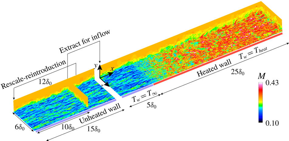
Schematic of the present direct numerical simulation of nominally zero-pressure-gradient heated transcritical and unheated non-transcritical flat-plate turbulent boundary layers. The origin of
 $x,y,z$
is at the inlet location of the wall-heated domain (right domain). Mach number (
 $M=\sqrt{u^{2}+v^{2}+w^{2}}/c_{s}$
) contours at side, cross and wall-parallel planes.

Figure 2 illustrates the computational set-up for the present DNS where the origin of
 $x$
is defined at the inlet location of the wall-heated domain (right domain in figure 2). The unheated non-transcritical turbulent boundary layer develops in the unheated domain. The rescaling–reintroduction method of Urbin & Knight (Reference Urbin and Knight2001) is used to generate realistic inflow turbulence in the unheated domain with the recycling location taken as
 $12\unicode[STIX]{x1D6FF}_{0}$
downstream of the inflow:
 $\unicode[STIX]{x1D6FF}_{0}$
is approximately 99 % of the boundary layer thickness at the inlet location
 $x=0$
in the wall-heated domain, i.e. equivalent to
 $10\unicode[STIX]{x1D6FF}_{0}$
downstream of the inflow in the unheated domain. This unheated turbulent boundary layer is also used as the inflow generator for the DNS of the heated transcritical turbulent boundary layer in the wall-heated domain. Instantaneous flow at the location
 $10\unicode[STIX]{x1D6FF}_{0}$
downstream of the inflow in the unheated domain is extracted and imposed as the inflow conditions for the wall-heated domain in which the low-temperature fully developed turbulent boundary layer is heated by the high-temperature isothermal wall. In the domain of the heated transcritical turbulent boundary layer, the region of
 $0\leqslant x/\unicode[STIX]{x1D6FF}_{0}<5-10\unicode[STIX]{x0394}x/\unicode[STIX]{x1D6FF}_{0}$
(where
 $\unicode[STIX]{x0394}x$
is the constant streamwise grid spacing) remains unheated at
 $T_{w}=T_{\infty }=25$
K, and the heated wall condition at the fixed wall temperature of
 $T_{w}=T_{heat}=100$
or 200 K is imposed in the region of
 $x/\unicode[STIX]{x1D6FF}_{0}>5+10\unicode[STIX]{x0394}x/\unicode[STIX]{x1D6FF}_{0}$
. In the range
 $5-10\unicode[STIX]{x0394}x/\unicode[STIX]{x1D6FF}_{0}\leqslant x/\unicode[STIX]{x1D6FF}_{0}\leqslant 5+10\unicode[STIX]{x0394}x/\unicode[STIX]{x1D6FF}_{0}$
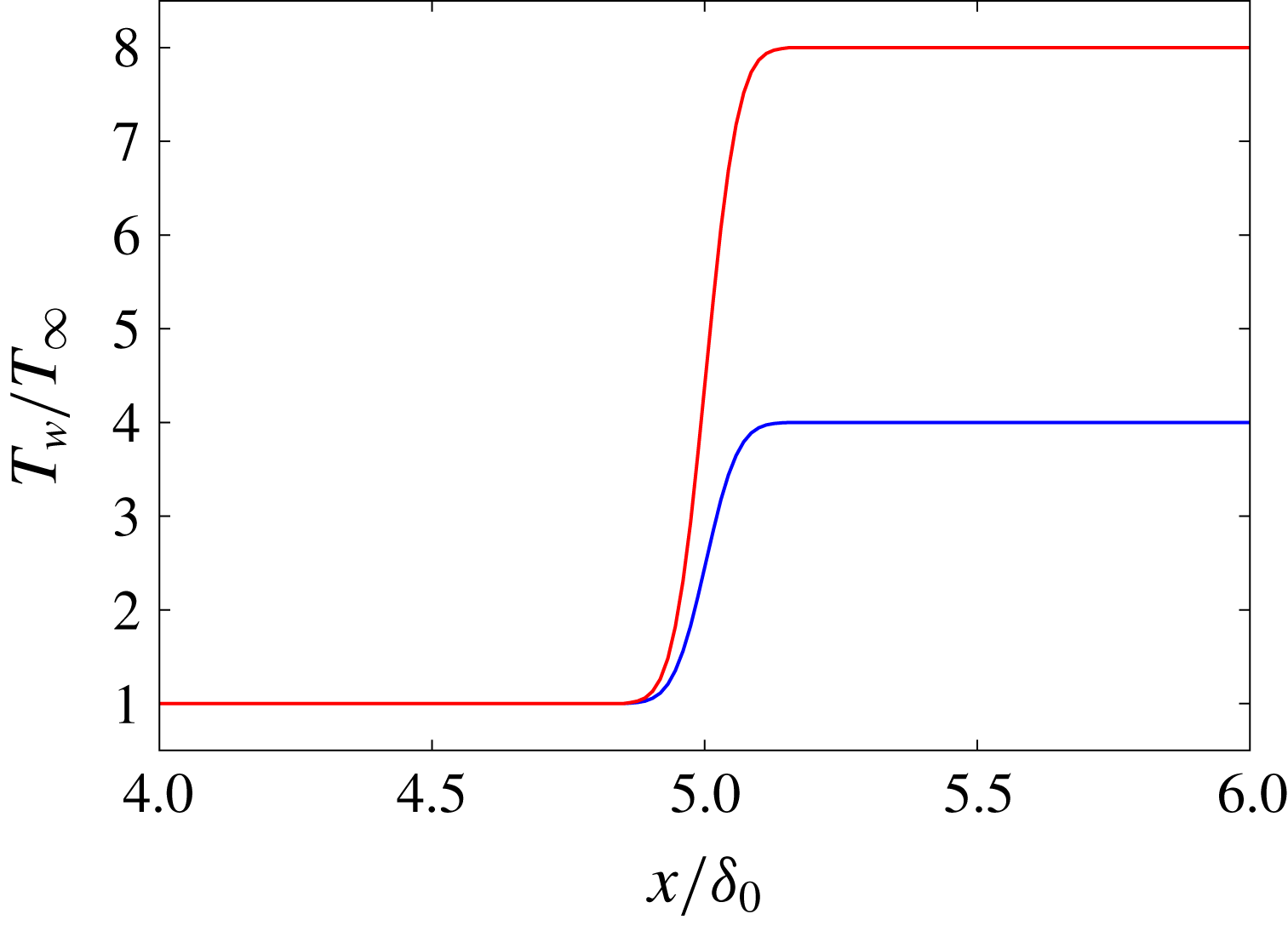
, to avoid a discontinuity in the wall temperature, the wall temperature increases as a smoothed step change from
 $T_{w}=T_{\infty }$
to
 $T_{heat}$
as shown in figure 3 using the error function:
 $$\begin{eqnarray}\displaystyle & \displaystyle T_{w}=(1-f)T_{\infty }+fT_{heat}, & \displaystyle\end{eqnarray}$$
 $$\begin{eqnarray}\displaystyle & \displaystyle f=0.5(\text{erf}(0.21(x-5)/\unicode[STIX]{x0394}x)+1.0). & \displaystyle\end{eqnarray}$$
Wall-temperature conditions in the wall-heated computational domain. Blue,
 $T_{heat}=100$
K; red,
 $T_{heat}=200$
K.

The size of the computational test section for the unheated domain is
 $L_{x}=15\unicode[STIX]{x1D6FF}_{0}$
,
 $L_{y}=2.4\unicode[STIX]{x1D6FF}_{0}$
and
 $L_{z}=6\unicode[STIX]{x1D6FF}_{0}$
in the streamwise (
 $x$
), wall-normal (
 $y$
) and spanwise (
 $z$
) directions. Additional buffer regions with lengths of
 $L_{x,buf}=10\unicode[STIX]{x1D6FF}_{0}$
and
 $L_{y,buf}=10\unicode[STIX]{x1D6FF}_{0}$
are placed at the outlet and upper boundaries to remove turbulent fluctuations and any reflections from the boundaries. The grid is smoothly stretched in the buffer regions toward the boundaries, thus coarsening the mesh toward the boundaries. The size of the test section for the heated boundary layer domain extends to
 $L_{x}=30\unicode[STIX]{x1D6FF}_{0}$
,
 $L_{y}=2.4\unicode[STIX]{x1D6FF}_{0}$
and
 $L_{z}=6\unicode[STIX]{x1D6FF}_{0}$
, and buffer regions with lengths of
 $L_{x,buf}=50\unicode[STIX]{x1D6FF}_{0}$
and
 $L_{y,buf}=6.6\unicode[STIX]{x1D6FF}_{0}$
are placed at the outlet and upper boundaries. The wall boundary condition is the isothermal no-slip condition, and the periodic boundary condition is imposed in the spanwise direction.
The Reynolds numbers for the unheated non-transcritical turbulent boundary layers at
 $10\unicode[STIX]{x1D6FF}_{0}$
downstream of the inlet in the unheated domain (i.e. equivalent to the inlet of the heated domain) for both the 2 and 4 MPa pressure conditions are
 $Re_{\unicode[STIX]{x1D703}}\equiv \unicode[STIX]{x1D70C}_{\infty }u_{\infty }\unicode[STIX]{x1D703}/\unicode[STIX]{x1D707}_{\infty }\approx 1010$
where
 $\unicode[STIX]{x1D703}$
is the momentum thickness and
 $Re_{\unicode[STIX]{x1D70F}}\equiv \unicode[STIX]{x1D70C}_{w}u_{\unicode[STIX]{x1D70F}}\unicode[STIX]{x1D6FF}/\unicode[STIX]{x1D707}_{w}\approx 390$
where
 $u_{\unicode[STIX]{x1D70F}}=\sqrt{\unicode[STIX]{x1D70F}_{w}/\unicode[STIX]{x1D70C}_{w}}$
. The Reynolds numbers for the heated transcritical turbulent boundary layers at
 $x=25\unicode[STIX]{x1D6FF}_{0}$
in the heated domain are
 $Re_{\unicode[STIX]{x1D703}}\approx 1500$
and 1600, and
 $Re_{\unicode[STIX]{x1D70F}}\approx$
210 and 90 at
 $p=2$
MPa for
 $T_{w}=100$
and 200 K conditions, respectively, and
 $Re_{\unicode[STIX]{x1D703}}\approx 1500$
and 1600, and
 $Re_{\unicode[STIX]{x1D70F}}\approx 360$
and 150 at
 $p=4$
MPa for
 $T_{w}=100$
and 200 K. Since the dynamic viscosity
 $\unicode[STIX]{x1D707}/\unicode[STIX]{x1D70C}$
gradually increases with increasing temperature at
 $T>T_{pc}$
as indicated in figure 1,
 $Re_{\unicode[STIX]{x1D70F}}$
becomes higher in the unheated non-transcritical boundary layers.
2.3 Characteristic length scales and grid convergence
There are several characteristic length scales for the turbulent boundary layer with variable thermodynamic and fluid transport properties as considered in this study. The conventional wall scaling uses the viscous length scale
 $\unicode[STIX]{x1D6FF}_{v}=\unicode[STIX]{x1D707}_{w}/(\unicode[STIX]{x1D70C}_{w}\,u_{\unicode[STIX]{x1D70F}})$
where the friction velocity
 $u_{\unicode[STIX]{x1D70F}}=\sqrt{\unicode[STIX]{x1D70F}_{w}/\unicode[STIX]{x1D70C}_{w}}$
to characterize the inner layer:
 $\unicode[STIX]{x1D6FF}_{v}$
is essentially the inverse of the friction Reynolds number
 $\unicode[STIX]{x1D6FF}_{v}=\unicode[STIX]{x1D6FF}/Re_{\unicode[STIX]{x1D70F}}$
which leads a smaller viscous length scale with a higher friction Reynolds number. By considering the variations in mean density and shear viscosity, Huang, Coleman & Bradshaw (Reference Huang, Coleman and Bradshaw1995) proposed to use the semi-local viscous length scale
 $\unicode[STIX]{x1D6FF}_{v}^{\ast }=\unicode[STIX]{x1D707}/(\unicode[STIX]{x1D70C}\,u_{\unicode[STIX]{x1D70F}}^{\ast })$
where
 $u_{\unicode[STIX]{x1D70F}}^{\ast }$
is the semi-local friction velocity defined by
 $u_{\unicode[STIX]{x1D70F}}^{\ast }=\sqrt{\unicode[STIX]{x1D70F}_{w}/\unicode[STIX]{x1D70C}}$
to characterize the inner layer with variable properties. They found that the semi-locally scaled wall distance
 $y^{\ast }=y/\unicode[STIX]{x1D6FF}_{v}^{\ast }$
instead of using the conventional
 $y^{+}=y/\unicode[STIX]{x1D6FF}_{v}$
shows a better collapse of turbulence statistics in boundary layers with variable properties. The semi-local friction Reynolds number is defined as
 $Re_{\unicode[STIX]{x1D70F}}^{\ast }\equiv \unicode[STIX]{x1D70C}\,u_{\unicode[STIX]{x1D70F}}^{\ast }\unicode[STIX]{x1D6FF}/\unicode[STIX]{x1D707}=(\unicode[STIX]{x1D70C}/\unicode[STIX]{x1D70C}_{w})^{0.5}\unicode[STIX]{x1D707}_{w}/\unicode[STIX]{x1D707}Re_{\unicode[STIX]{x1D70F}}$
, and
 $\unicode[STIX]{x1D6FF}_{v}^{\ast }$
is the inverse of the semi-local friction Reynolds number
 $\unicode[STIX]{x1D6FF}_{v}^{\ast }=\unicode[STIX]{x1D6FF}/Re_{\unicode[STIX]{x1D70F}}^{\ast }$
. This relation leads to a smaller
 $\unicode[STIX]{x1D6FF}_{v}^{\ast }$
at a higher
 $Re_{\unicode[STIX]{x1D70F}}^{\ast }$
. The smallest scales in turbulent flows (the velocity field) can be characterized by the Kolmogorov microscale
 $\unicode[STIX]{x1D702}_{k}\equiv ((\overline{\unicode[STIX]{x1D707}}/\overline{\unicode[STIX]{x1D70C}})^{3}/\unicode[STIX]{x1D716})^{0.25}$
that is a function of the local mean density, shear viscosity and the dissipation rate of turbulent kinetic energy
 $\unicode[STIX]{x1D716}$
. The smallest scale of the temperature field is defined by the function of local Prandtl number and the Kolmogorov scale as
 $\unicode[STIX]{x1D702}_{\unicode[STIX]{x1D703}}\equiv \unicode[STIX]{x1D702}_{k}Pr^{-0.5}$
(Zonta, Marchioli & Soldati Reference Zonta, Marchioli and Soldati2012).
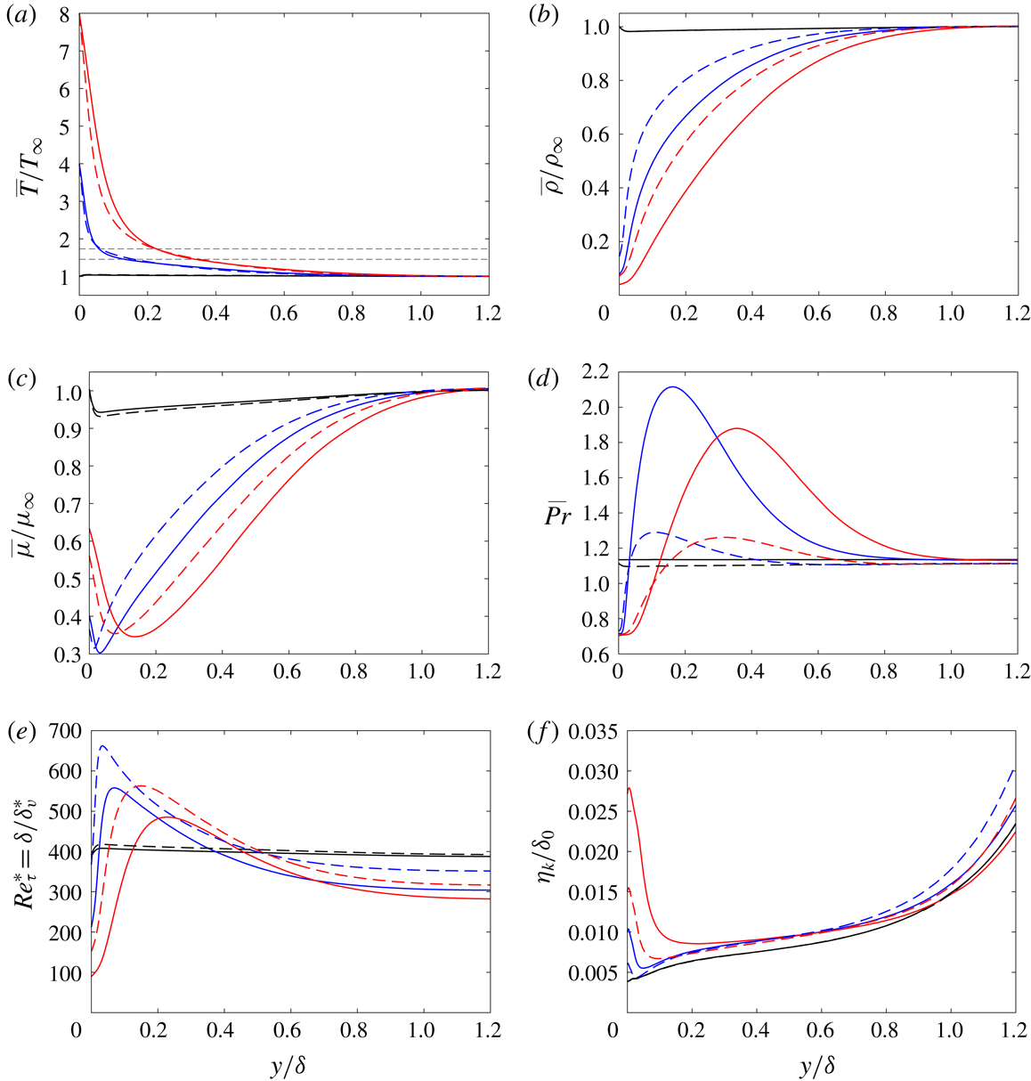
Distributions of mean (a) temperature, (b) density, (c) shear viscosity, (d) Prandtl number
 $\overline{Pr}=\overline{c_{p}}\,\overline{\unicode[STIX]{x1D707}}/\overline{\unicode[STIX]{x1D705}}$
, (e) semi-local friction Reynolds number and (f) Kolmogorov microscale in the heated transcritical and unheated non-transcritical turbulent boundary layers. The data are obtained at
 $x=25\unicode[STIX]{x1D6FF}_{0}$
for heated cases and
 $10\unicode[STIX]{x1D6FF}_{0}$
downstream of the inlet for unheated cases with the spatial resolutions of grids A1 and A2 in table 1. Black,
 $T_{w}=T_{\infty }=25~\text{K}$
; blue,
 $T_{w}=100~\text{K}$
; red,
 $T_{w}=200~\text{K}$
; solid lines,
 $p=2$
MPa; dashed lines
 $p=4$
MPa. Thin grey dashed lines in (a) pseudo-critical temperature
 $\overline{T}/T_{\infty }\approx 1.46$
and 1.73 at
 $p=2$
and 4 MPa.

Figure 4 shows the mean variable properties and the characteristic length scales within the heated transcritical and unheated non-transcritical boundary layers. In the following,
 $\overline{f}$
and
 $\widetilde{f}$
denote the Reynolds and Favre averaging quantities where
 $f=\overline{f}+f^{\prime }$
and
 $f=\widetilde{f}+f^{\prime \prime }$
. In the heated boundary layers, the mean temperature varies through
 $T_{pc}$
within the boundary layer where the pseudo-critical temperatures at
 $p=2$
and 4 MPa for parahydrogen are approximately 36.4 and 43.3 K (
 $T/T_{\infty }\approx 1.46$
and 1.73), respectively, and thus the transcritical condition (i.e. the pseudo-boiling process) exists within the heated boundary layers. On the other hand, an approximately constant temperature (
 $\overline{T}\approx 25~\text{K}$
) and constant variable properties are obtained for the unheated boundary layers. Since the thermodynamic and fluid transport properties vary abruptly within a narrow temperature range across
 $T_{pc}$
as shown in figure 1, significant variations in the mean thermodynamic and fluid transport properties are observed in the heated transcritical boundary layers, which lead to the variations in the characteristic length scales within the boundary layers. For the heated transcritical boundary layers, in the most severe case (
 $T_{w}=T_{heat}=200$
K and
 $p=2$
MPa), the mean density varies more than 20 times from the low density at the wall (
 $\overline{\unicode[STIX]{x1D70C}}_{w}/\unicode[STIX]{x1D70C}_{\infty }\approx 0.04$
) to the free stream. The local mean Prandtl number
 $\overline{Pr}$
increases toward the transcritical condition (similar profiles are also obtained by the specific heat at constant pressure
 $\overline{c_{p}}$
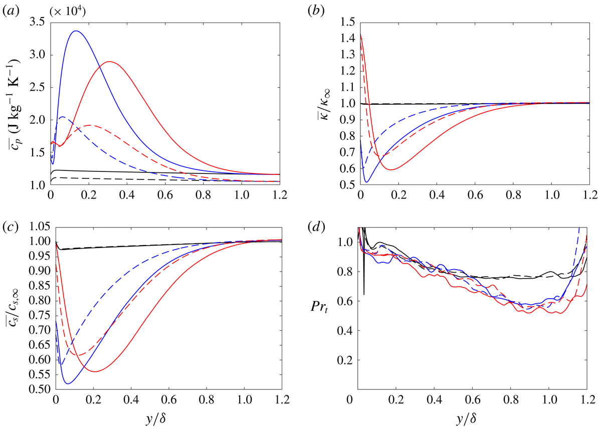
as shown in appendix A), and
 $\overline{Pr}>1$
in most of the regions, resulting in
 $\unicode[STIX]{x1D702}_{\unicode[STIX]{x1D703}}<\unicode[STIX]{x1D702}_{k}$
except near the heated wall. According to figure 1, the mean shear viscosity
 $\overline{\unicode[STIX]{x1D707}}$
(and also the mean thermal conductivity
 $\overline{\unicode[STIX]{x1D705}}$
in appendix A) reaches its minimum value at the high-temperature side (i.e. near-wall side) of the transcritical condition. We note that the mean thermodynamic and fluid transport properties do not recover to the free-stream values immediately through the mean-temperature-based transcritical region
 $\overline{T}\approx T_{pc}$
. This is primarily because the variable properties are not a linear function of
 $T$
for supercritical fluids as shown in figure 1. For example, if one considers the density as a function of
 $\unicode[STIX]{x1D70C}=f(T,p)$
,
 $\overline{\unicode[STIX]{x1D70C}}\neq f(\overline{T},\overline{p})$
when
 $T^{\prime }\neq 0$
. The highest friction Reynolds number
 $Re_{\unicode[STIX]{x1D70F}}$
(equivalent to
 $Re_{\unicode[STIX]{x1D70F}}^{\ast }$
at the wall) and thus the smallest viscous length scale
 $\unicode[STIX]{x1D6FF}_{v}$
(
 $=\unicode[STIX]{x1D6FF}/Re_{\unicode[STIX]{x1D70F}}$
) are obtained by the unheated cases. The semi-local Reynolds number
 $Re_{\unicode[STIX]{x1D70F}}^{\ast }$
(
 $=(\overline{\unicode[STIX]{x1D70C}}/\overline{\unicode[STIX]{x1D70C}_{w}})^{0.5}\overline{\unicode[STIX]{x1D707}_{w}}/\overline{\unicode[STIX]{x1D707}}\,Re_{\unicode[STIX]{x1D70F}}$
) for the heated cases is low near the wall, which essentially means relatively large semi-local viscous length scale
 $\unicode[STIX]{x1D6FF}_{v}^{\ast }$
(
 $=\unicode[STIX]{x1D6FF}/Re_{\unicode[STIX]{x1D70F}}^{\ast }$
) near the wall. However, for the heated cases,
 $Re_{\unicode[STIX]{x1D70F}}^{\ast }$
increases away from the wall and attains a higher
 $Re_{\unicode[STIX]{x1D70F}}^{\ast }$
and thus smaller
 $\unicode[STIX]{x1D6FF}_{v}^{\ast }$
around the transcritical condition compared to the unheated cases. Similar length scale variation is also observed in the Kolmogorov scales
 $\unicode[STIX]{x1D702}_{k}$
for the heated cases, a larger
 $\unicode[STIX]{x1D702}_{k}$
near the heated wall and reduced
 $\unicode[STIX]{x1D702}_{k}$
toward around the transcritical condition. Although not shown here, the smallest scales of the temperature field
 $\unicode[STIX]{x1D702}_{\unicode[STIX]{x1D703}}$
(
 $=\unicode[STIX]{x1D702}_{k}\overline{Pr}^{-0.5}$
) behave similarly to
 $\unicode[STIX]{x1D702}_{k}$
. For the heated cases,
 $\unicode[STIX]{x1D702}_{\unicode[STIX]{x1D703}}>\unicode[STIX]{x1D702}_{k}$
near the wall where
 $\overline{Pr}<1$
and
 $\unicode[STIX]{x1D702}_{\unicode[STIX]{x1D703}}<\unicode[STIX]{x1D702}_{k}$
away from the wall, whereas
 $\unicode[STIX]{x1D702}_{\unicode[STIX]{x1D703}}<\unicode[STIX]{x1D702}_{k}$
for the unheated cases.
Grid sensitivity study for the heated transcritical and unheated non-transcritical turbulent boundary layers at
 $p=4$
MPa and
 $T_{w}=25$
and 100 K.
 $N_{x}$
,
 $N_{y}$
,
 $N_{z}$
, number of grid points;
 $\unicode[STIX]{x0394}x^{+}$
,
 $\unicode[STIX]{x0394}y^{+}$
,
 $\unicode[STIX]{x0394}z^{+}$
, grid resolution in wall units (normalized by the viscous length scale
 $\unicode[STIX]{x1D6FF}_{v}$
);
 $\unicode[STIX]{x0394}x^{\ast }$
,
 $\unicode[STIX]{x0394}y^{\ast }$
,
 $\unicode[STIX]{x0394}z^{\ast }$
, grid resolution in semi-local wall units (normalized by the semi-local viscous length scale
 $\unicode[STIX]{x1D6FF}_{v}^{\ast }$
):
 $\unicode[STIX]{x0394}x/\unicode[STIX]{x1D6FF}_{0}$
,
 $\unicode[STIX]{x0394}y/\unicode[STIX]{x1D6FF}_{0}$
and
 $\unicode[STIX]{x0394}z/\unicode[STIX]{x1D6FF}_{0}$
are the same between grid A1 and A2, and between grid B1 and B2.

Grid refinements by a factor of
 $\sqrt{2}$
in each direction are conducted based on the unheated non-transcritical (
 $T_{w}=25$
K) and heated transcritical (
 $T_{w}=100$
K) turbulent boundary layers at the
 $p=4$
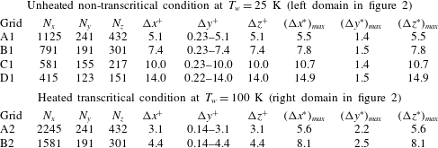
MPa condition. Table 1 summarizes the number of grid points and the grid resolution in wall units used for the grid refinement study (in which
 $\unicode[STIX]{x0394}x/\unicode[STIX]{x1D6FF}_{0}$
,
 $\unicode[STIX]{x0394}y/\unicode[STIX]{x1D6FF}_{0}$
and
 $\unicode[STIX]{x0394}z/\unicode[STIX]{x1D6FF}_{0}$
are the same between grid A1 and A2, and between grid B1 and B2). The grid resolution is based on the quantities at the
 $10\unicode[STIX]{x1D6FF}_{0}$
downstream location of the inlet for the unheated case and at
 $x=25\unicode[STIX]{x1D6FF}_{0}$
for the heated case. The chosen unheated case yields the highest Reynolds number
 $Re_{\unicode[STIX]{x1D70F}}$
, and the heated case yields the highest semi-local Reynolds number
 $Re_{\unicode[STIX]{x1D70F}}^{\ast }$
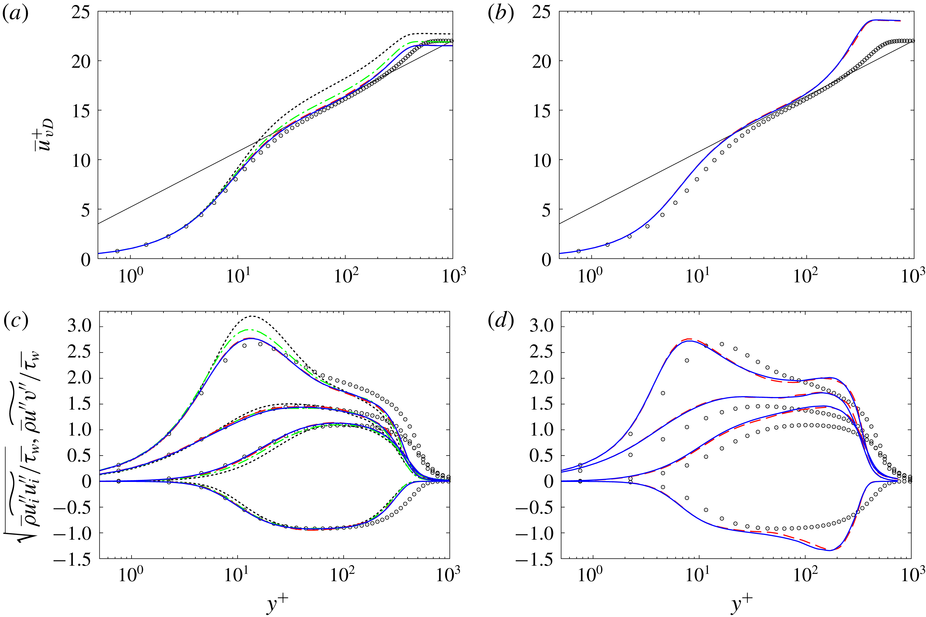
among all the cases. The mean streamwise velocity profile in a semi-logarithmic plot using the van Driest transformation
 $\overline{u}_{vD}^{+}=\int _{0}^{\overline{u}^{+}}(\overline{\unicode[STIX]{x1D70C}}/\overline{\unicode[STIX]{x1D70C}_{w}})^{1/2}\,\text{d}\overline{u}^{+}$
(Van Driest Reference Van Driest1951) and the Reynolds stresses are plotted in figure 5. The DNS data of the incompressible perfect-gas turbulent boundary layer at
 $Re_{\unicode[STIX]{x1D703}}=1410$
by Spalart (Reference Spalart1988) and the logarithmic scaling
 $\overline{u}_{vD}^{+}=(1/0.41)\log (y^{+})+5.2$
are also included in the figure for comparison. There is clearly a convergence process; arguably grids A1 or B1 for the unheated case and grids A2 or B2 for the heated case are needed for grid convergence in these quantities. The unheated non-transcritical turbulent boundary layer is in good agreement with the incompressible constant-property DNS with perfect-gas law (the discrepancies in the shorter logarithmic region and in the wake region are considered to be because of the lower Reynolds number
 $Re_{\unicode[STIX]{x1D703}}\approx 1010$
employed in this study). Because of the unheated non-transcritical and
 $M_{\infty }=0.3$
conditions, the thermodynamic and fluid transport properties are almost constant throughout the unheated non-transcritical boundary layer, as shown in figure 4, and also the fluctuating dilatation
 $\unicode[STIX]{x2202}u_{i}^{\prime }/\unicode[STIX]{x2202}x_{i}$
is negligibly small (this will be discussed in § 3.3). Because of these constant properties and negligible dilatation, the statistics obtained from the unheated non-transcritical boundary layer agree well with the incompressible DNS. In terms of the Kolmogorov microscale
 $\unicode[STIX]{x1D702}_{k}$
and the smallest scale of the temperature field
 $\unicode[STIX]{x1D702}_{\unicode[STIX]{x1D703}}$
, the grid resolutions of grid A1 for the unheated case are
 $\unicode[STIX]{x0394}x=\unicode[STIX]{x0394}z\lesssim 3.6\unicode[STIX]{x1D702}_{k}$
and
 ${\lesssim}3.8\unicode[STIX]{x1D702}_{\unicode[STIX]{x1D703}}$
, and the wall-normal grid spacing varies from a minimum value
 $\unicode[STIX]{x0394}y_{min}\lesssim 0.16\unicode[STIX]{x1D702}_{k}$
and
 ${\lesssim}0.17\unicode[STIX]{x1D702}_{\unicode[STIX]{x1D703}}$
at the wall to a value
 $\unicode[STIX]{x0394}y_{\unicode[STIX]{x1D6FF}}\lesssim 0.91\unicode[STIX]{x1D702}_{k}$
and
 ${\lesssim}0.96\unicode[STIX]{x1D702}_{\unicode[STIX]{x1D703}}$
at
 $y=\unicode[STIX]{x1D6FF}$
. The grid A2 for the heated case is
 $\unicode[STIX]{x0394}x=\unicode[STIX]{x0394}z\lesssim 3.2\unicode[STIX]{x1D702}_{k}$
and
 ${\lesssim}3.3\unicode[STIX]{x1D702}_{\unicode[STIX]{x1D703}}$
,
 $\unicode[STIX]{x0394}y_{min}\lesssim 0.10\unicode[STIX]{x1D702}_{k}$
and
 ${\lesssim}0.09\unicode[STIX]{x1D702}_{\unicode[STIX]{x1D703}}$
and
 $\unicode[STIX]{x0394}y_{\unicode[STIX]{x1D6FF}}\lesssim 0.76\unicode[STIX]{x1D702}_{k}$
and
 ${\lesssim}0.80\unicode[STIX]{x1D702}_{\unicode[STIX]{x1D703}}$
. These values are within the resolution requirements reported in prior DNS studies,
 $\unicode[STIX]{x0394}x<12\min \{\unicode[STIX]{x1D702}_{k},\unicode[STIX]{x1D702}_{\unicode[STIX]{x1D703}}\}$
,
 $\unicode[STIX]{x0394}y<2\min \{\unicode[STIX]{x1D702}_{k},\unicode[STIX]{x1D702}_{\unicode[STIX]{x1D703}}\}$
,
 $\unicode[STIX]{x0394}z<6\min \{\unicode[STIX]{x1D702}_{k},\unicode[STIX]{x1D702}_{\unicode[STIX]{x1D703}}\}$
(Zonta et al.
Reference Zonta, Marchioli and Soldati2012; Lee et al.
Reference Lee, Jung, Sung and Zaki2013; Patel, Boersma & Pecnik Reference Patel, Boersma and Pecnik2016). Also, as will be shown in table 3, we note that grids A1 and A2 fulfil the DNS resolution requirements for all the cases employed in this study.
Sensitivity of turbulence statistics to mesh resolution in the unheated non-transcritical and heated transcritical boundary layers at
 $p=4$
MPa and
 $T_{w}=25$
K (a,c) and 100 K (b,d). (a,b) The van Driest transformed mean streamwise velocity, (c,d) Reynolds stresses: upper lines,
 $\sqrt{\overline{\unicode[STIX]{x1D70C}}\widetilde{u^{\prime \prime }u^{\prime \prime }}/\overline{\unicode[STIX]{x1D70F}_{w}}}$
; upper-middle lines,
 $\sqrt{\overline{\unicode[STIX]{x1D70C}}\widetilde{w^{\prime \prime }w^{\prime \prime }}/\overline{\unicode[STIX]{x1D70F}_{w}}}$
; lower-middle lines,
 $\sqrt{\overline{\unicode[STIX]{x1D70C}}\widetilde{v^{\prime \prime }v^{\prime \prime }}/\overline{\unicode[STIX]{x1D70F}_{w}}}$
; lower lines,
 $\overline{\unicode[STIX]{x1D70C}}\widetilde{u^{\prime \prime }v^{\prime \prime }}/\overline{\unicode[STIX]{x1D70F}_{w}}$
. Blue solid lines, grids A1 and A2; red dashed lines, grids B1 and B2; green dashed-dotted lines, grid C1; black dotted lines, grid D1; circles, incompressible perfect-gas DNS by Spalart (Reference Spalart1988) at
 $Re_{\unicode[STIX]{x1D703}}=1410$
; thin grey line in (a,b),
 $\overline{u}_{vD}^{+}=1/0.41\log (y^{+})+5.2$
.

2.4 Spanwise domain extent
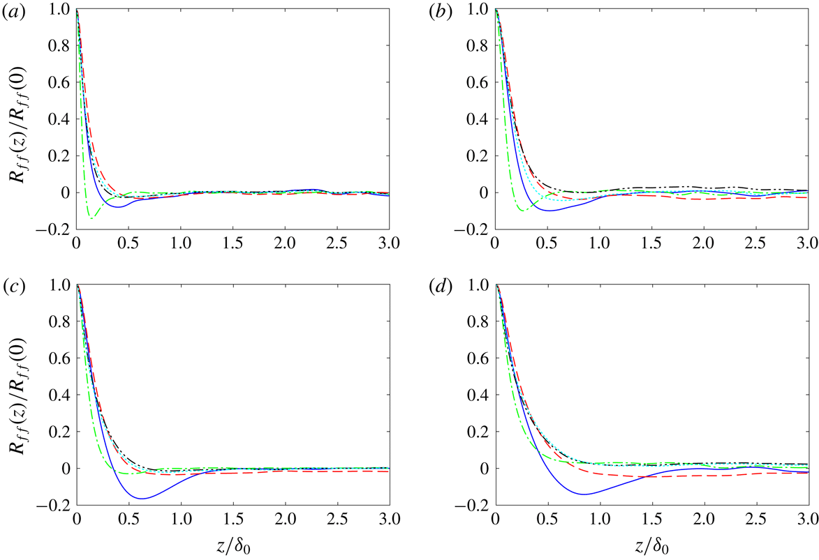
Two-point auto-correlation profiles in the spanwise direction at inner- and outer-layer locations. The data are obtained at
 $10\unicode[STIX]{x1D6FF}_{0}$
downstream of the inlet in the unheated domain
 $T_{w}=25~\text{K}$
(a,c) and at
 $x=25\unicode[STIX]{x1D6FF}_{0}$
in the heated domain
 $T_{w}=200~\text{K}$
(b,d) at
 $p=2$
MPa. (a,b) At
 $y/\unicode[STIX]{x1D6FF}\approx 0.1$
and
 $y^{+}\approx 39.4$
for
 $T_{w}=25~\text{K}$
, and
 $y/\unicode[STIX]{x1D6FF}\approx 0.1$
and
 $y^{+}\approx 9.2$
for
 $T_{w}=200~\text{K}$
; (c,d) at
 $y/\unicode[STIX]{x1D6FF}\approx 0.5$
and
 $y^{+}\approx 192.9$
for
 $T_{w}=25~\text{K}$
, and
 $y/\unicode[STIX]{x1D6FF}\approx 0.5$
and
 $y^{+}\approx 44.9$
for
 $T_{w}=200~\text{K}$
. Blue solid lines,
 $R_{uu}$
; green dashed-dotted lines,
 $R_{vv}$
; red dashed lines,
 $R_{ww}$
; black dashed double-dotted lines,
 $R_{\unicode[STIX]{x1D70C}\unicode[STIX]{x1D70C}}$
; cyan dotted lines,
 $R_{TT}$
.

Although a relatively large spanwise domain size (
 $L_{z}=6\unicode[STIX]{x1D6FF}_{0}$
) is employed in this study, the two-point auto-correlation function in the homogeneous spanwise direction is analysed to validate the spanwise domain extent. The spanwise auto-correlation coefficients
 $R_{ff}(z)/R_{ff}(0)$
in the inner and outer layers computed at the grid resolutions of A1 and A2 are shown in figure 6. The coefficients are computed at
 $10\unicode[STIX]{x1D6FF}_{0}$
downstream of the inlet in the unheated domain
 $T_{w}=25~\text{K}$
and at
 $x=25\unicode[STIX]{x1D6FF}_{0}$
in the heated domain
 $T_{w}=200~\text{K}$
at a supercritical pressure of
 $p=2$
MPa, where the heated case shows the maximum boundary layer growth, as shown in table 2. The correlation function is defined as
 $$\begin{eqnarray}\displaystyle R_{ff}(z)=\mathop{\sum }_{k=1}^{N_{z}-1}\overline{f_{k}f_{k+k_{r}}},\quad k_{r}=0,1,\ldots ,k-1, & & \displaystyle\end{eqnarray}$$
where
 $z=k_{r}\unicode[STIX]{x0394}z$
,
 $f=u^{\prime },v^{\prime },w^{\prime },\unicode[STIX]{x1D70C}^{\prime },T^{\prime }$
and
 $\overline{(\cdot )}$
denotes the averaging of more than 4750 sample flow fields that are periodically stored at the time interval of
 $4.8\times 10^{-2}\unicode[STIX]{x1D6FF}_{0}/u_{\infty }$
to ensure the convergence of the correlation functions. The two-point correlations are sufficiently decorrelated over a distance of
 $L_{z}/2$
and decay toward zero around
 $z/\unicode[STIX]{x1D6FF}_{0}\lesssim 1.5$
in the inner layer and
 $z/\unicode[STIX]{x1D6FF}_{0}\lesssim 2$
in the outer layer. This ensures that the spanwise domain size is sufficient not to affect the turbulence dynamics.
Based on the studies of the spatial resolution and spanwise domain extent, the grids A1 and A2 with the spanwise domain extent of
 $L_{z}=6\unicode[STIX]{x1D6FF}_{0}$
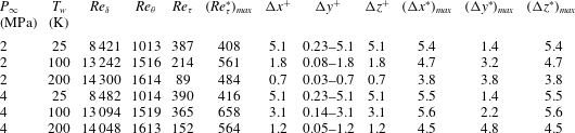
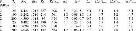
are used for the rest of the study. Tables 2 and 3 summarizes the Reynolds numbers and spatial resolutions for the present DNS database. The employed spatial resolution is comparable to that used in prior DNS studies (Zonta et al.
Reference Zonta, Marchioli and Soldati2012; Lee et al.
Reference Lee, Jung, Sung and Zaki2013; Patel et al.
Reference Patel, Boersma and Pecnik2016).
Reynolds number, spatial resolutions in wall units (normalized by the viscous length scale
 $\unicode[STIX]{x1D6FF}_{v}$
) and maximum spatial resolution normalized by the semi-local viscous length scale
 $\unicode[STIX]{x1D6FF}_{v}^{\ast }$
at
 $10\unicode[STIX]{x1D6FF}_{0}$
downstream of the inlet for the unheated cases (
 $T_{w}=25$
K) and at
 $x=25\unicode[STIX]{x1D6FF}_{0}$
for the heated cases (
 $T_{w}=100$
and 200 K) of the present DNS database.
Maximum spatial resolution normalized by the Kolmogorov scale
 $\unicode[STIX]{x1D702}_{k}$
and the smallest scale of the temperature field
 $\unicode[STIX]{x1D702}_{\unicode[STIX]{x1D703}}\equiv \unicode[STIX]{x1D702}_{k}\overline{Pr}^{-0.5}$
(Zonta et al.
Reference Zonta, Marchioli and Soldati2012) at
 $10\unicode[STIX]{x1D6FF}_{0}$
downstream of the inlet for the unheated cases (
 $T_{w}=25$
K) and at
 $x=25\unicode[STIX]{x1D6FF}_{0}$
for the heated cases (
 $T_{w}=100$
and 200 K) of the present DNS database. Subscript
 $\unicode[STIX]{x1D6FF}$
denotes value at
 $y=\unicode[STIX]{x1D6FF}$
.

3 Turbulence statistics
For the unheated non-transcritical turbulent boundary layers at
 $T_{w}=T_{\infty }=25~\text{K}$
, the turbulence statistics discussed below are obtained at
 $10\unicode[STIX]{x1D6FF}_{0}$
downstream of the inlet in the unheated domain (left domain in figure 2), i.e. equivalent to the inlet location of the heated domain, unless otherwise noted. With the heated isothermal wall (right domain in figure 2), the transient and adaptation processes of the boundary layer to the heated isothermal wall conditions are observed where the wall temperature is increased steeply around
 $x=5\unicode[STIX]{x1D6FF}_{0}$
as in figure 3. In the present study, to investigate the heated transcritical turbulent boundary layers after the adaptation process, the turbulence statistics at the
 $x/\unicode[STIX]{x1D6FF}_{0}=25$
location in the heated domain are discussed for the heated cases
 $T_{w}=T_{heat}=100$
and
 $200~\text{K}$
. The statistical properties of the flow are computed by averaging in time for a time interval of more than
 $280\unicode[STIX]{x1D6FF}_{0}/u_{\infty }$
as well as in the homogeneous spanwise direction to ensure convergence of flow statistics.
3.1 Variances of thermodynamic and fluid transport properties
Variances of density and shear viscosity for the heated transcritical and unheated non-transcritical turbulent boundary layers in the outer scaling
 $y/\unicode[STIX]{x1D6FF}$
(a,c) and semi-local inner scaling
 $y^{\ast }$
with a semi-logarithmic plot (b,d): (a,b) local density fluctuations
 $\sqrt{\overline{\unicode[STIX]{x1D70C}^{\prime }\unicode[STIX]{x1D70C}^{\prime }}}/\overline{\unicode[STIX]{x1D70C}}$
, (c,d) local shear viscosity fluctuations
 $\sqrt{\overline{\unicode[STIX]{x1D707}^{\prime }\unicode[STIX]{x1D707}^{\prime }}}/\overline{\unicode[STIX]{x1D707}}$
. Lines as in figure 4.

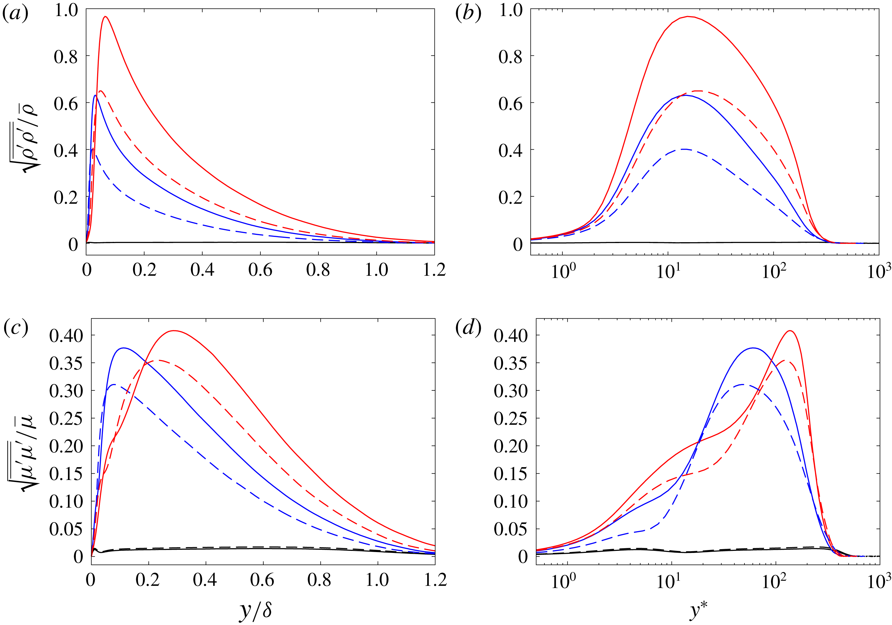
Variances of the density and shear viscosity relative to the local mean value in the outer scaling
 $y/\unicode[STIX]{x1D6FF}$
and semi-local inner scaling
 $y^{\ast }$
are plotted in figure 7. Similar to the finding of Huang et al. (Reference Huang, Coleman and Bradshaw1995), Patel et al. (Reference Patel, Peeters, Boersma and Pecnik2015), the semi-local inner-layer scaling
 $y^{\ast }$
improves the inner-layer scaling for the peak location compared to the conventional
 $y^{+}$
scaling (although the
 $y^{+}$
scaling is not shown here). The peak location of the density fluctuations shows a good collapse for the different wall heating and pressure conditions while the shear viscosity shows a collapse only for the different pressure conditions. Significant variances of the thermodynamic and fluid transport properties, especially density, are observed in the heated transcritical turbulent boundary layers, whereas the fluctuations are negligibly small in the unheated non-transcritical boundary layers. Although the speed of sound decreases around the transcritical condition for the heated cases as shown in appendix A, the turbulent Mach number and local Mach number are
 $\overline{M_{t}}\lesssim 0.08$
and
 $\overline{M}\lesssim 0.4$
throughout the boundary layers. The significant density and shear viscosity fluctuations originate from the effects of the abrupt density and shear viscosity variations with temperature at the transcritical condition where the density and shear viscosity varies abruptly within a very narrow temperature range through
 $T_{pc}$
as shown in figure 1. The density fluctuations reach
 $\sqrt{\overline{\unicode[STIX]{x1D70C}^{\prime }\unicode[STIX]{x1D70C}^{\prime }}}/\overline{\unicode[STIX]{x1D70C}}\approx 0.4{-}1.0$
near the wall, where the mean density gradient
 $\text{d}\overline{\unicode[STIX]{x1D70C}}/\text{d}y$
approximately reaches its maximum, and the variances of shear viscosity reach
 $\sqrt{\overline{\unicode[STIX]{x1D707}^{\prime }\unicode[STIX]{x1D707}^{\prime }}}/\overline{\unicode[STIX]{x1D707}}\approx 0.4$
. Although not shown, the variances of temperature relative to the mean local temperature become
 $\sqrt{\overline{T^{\prime }T^{\prime }}}/\overline{T}\approx 0.25{-}0.4$
. We note that to our knowledge no prior DNS of turbulent boundary layers at supercritical pressure has investigated this level of large density fluctuations
 $\sqrt{\overline{\unicode[STIX]{x1D70C}^{\prime }\unicode[STIX]{x1D70C}^{\prime }}}/\overline{\unicode[STIX]{x1D70C}}\approx 0.4{-}1.0$
involved in the flows. The large density fluctuations observed in the present DNS are primarily because the present study employs wider temperature ranges across the pseudo-critical temperature, and thus sharper density variations are induced within the boundary layers compared to the prior DNS studies (Bae et al.
Reference Bae, Yoo and Choi2005, Reference Bae, Yoo and Mceligot2008; Nemati et al.
Reference Nemati, Patel, Boersma and Pecnik2015, Reference Nemati, Patel, Boersma and Pecnik2016; Peeters et al.
Reference Peeters, Pecnik, van der Hagen and Boersma2016). We also note that
 $p=2$
MPa (which is closer to the critical pressure) cases show a higher peak in the fluctuations compared to
 $p=4$
MPa cases. This is related to the variations in the fluid properties as a function of temperature. The fluid property variations get steeper when the pressure approaches the critical pressure, as shown in figure 1. As will be discussed, the large density fluctuations in the heated transcritical boundary layers show a non-negligible impact on the near-wall turbulence and also induce the divergence of the velocity fluctuations
 $\unicode[STIX]{x2202}u_{i}^{\prime }/\unicode[STIX]{x2202}x_{i}$
.
Reynolds- and Favre-averaged mean (a) streamwise velocity and (b) wall-normal velocity for heated transcritical and unheated non-transcritical turbulent boundary layers at
 $p=2$
MPa. Black,
 $T_{w}=T_{\infty }=25~\text{K}$
; blue,
 $T_{w}=100~\text{K}$
; red,
 $T_{w}=200~\text{K}$
; solid lines, Reynolds-averaged velocity; dashed lines, Favre-averaged velocity.

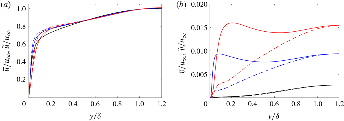
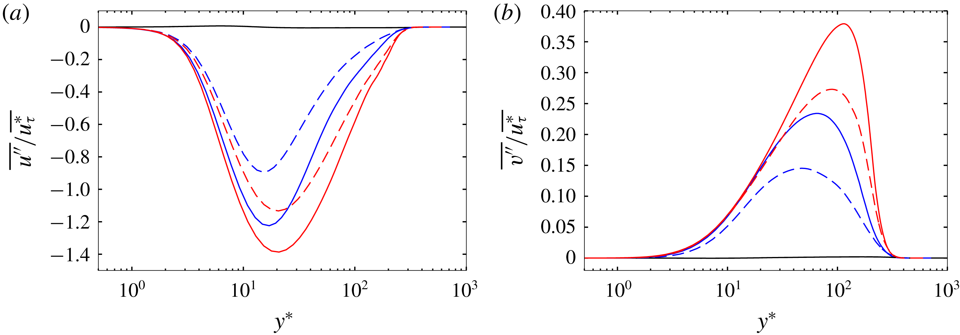
Figure 8 shows the Reynolds- and Favre-averaged mean streamwise and wall-normal velocities at
 $p=2$
MPa. For the heated cases, there is a distinct difference between the Reynolds- and Favre-averaged velocities, especially near the wall region, while
 $\overline{u_{i}}\approx \widetilde{u_{i}}$
in the unheated cases. The difference indicates the non-zero Favre-averaged velocity fluctuations
 $\overline{u_{i}^{\prime \prime }}$
of
 $$\begin{eqnarray}\displaystyle \overline{u_{i}}-\widetilde{u_{i}}=\overline{u_{i}^{\prime \prime }}=\overline{u_{i}}-\frac{\overline{(\overline{\unicode[STIX]{x1D70C}}+\unicode[STIX]{x1D70C}^{\prime })(\overline{u_{i}}+u_{i}^{\prime })}}{\overline{\unicode[STIX]{x1D70C}}}=-\frac{\overline{\unicode[STIX]{x1D70C}^{\prime }u_{i}^{\prime }}}{\overline{\unicode[STIX]{x1D70C}}}, & & \displaystyle\end{eqnarray}$$
and also indicates the generation of the turbulent mass flux
 $\unicode[STIX]{x1D70C}^{\prime }u_{i}^{\prime }$
in the heated transcritical boundary layers. We note that for the heated transcritical boundary layers non-negligible mean wall-normal velocity is generated near the wall whereas
 $\overline{v}\approx \widetilde{v}\approx 0$
for the unheated non-transcritical cases (as also seen in typical turbulent boundary layers). The non-negligible near-wall wall-normal velocity for the heated cases causes non-zero
 $-\overline{\unicode[STIX]{x1D70C}}\widetilde{u}\widetilde{v}$
near the wall in the streamwise stress-balance equation which is directly connected to the logarithmic law as will be discussed in § 3.2. The Reynolds-averaged near-wall wall-normal velocity
 $\overline{v}$
(
 $=\widetilde{v}+\overline{v^{\prime \prime }}=\widetilde{v}-\overline{\unicode[STIX]{x1D70C}^{\prime }v^{\prime }}/\overline{\unicode[STIX]{x1D70C}}$
) exceeds the Favre-averaged velocity for the heated cases, indicating a positive
 $\overline{v^{\prime \prime }}$
through the negative correlation between
 $\unicode[STIX]{x1D70C}^{\prime }$
and
 $v^{\prime }$
(and thus
 $-\overline{\unicode[STIX]{x1D70C}^{\prime }v^{\prime }}>0$
). Similarly the increased
 $\widetilde{u}$
compared to
 $\overline{u}$
in the near-wall region is caused by the negative
 $\overline{u^{\prime \prime }}$
due to the positive correlation between
 $\unicode[STIX]{x1D70C}^{\prime }$
and
 $u^{\prime }$
(
 $-\overline{\unicode[STIX]{x1D70C}^{\prime }u^{\prime }}<0$
). The mechanisms of the positive and negative correlations between
 $\unicode[STIX]{x1D70C}^{\prime }$
and
 $u^{\prime }$
and
 $v^{\prime }$
will be discussed in detail in § 4.
3.2 Logarithmic law of the wall and stress-balance equation
Through the generation of the turbulent mass flux
 $\unicode[STIX]{x1D70C}^{\prime }u_{i}^{\prime }$
(where
 $\overline{u_{i}}-\widetilde{u_{i}}=\overline{u_{i}^{\prime \prime }}=-\overline{\unicode[STIX]{x1D70C}^{\prime }u_{i}^{\prime }}/\overline{\unicode[STIX]{x1D70C}}$
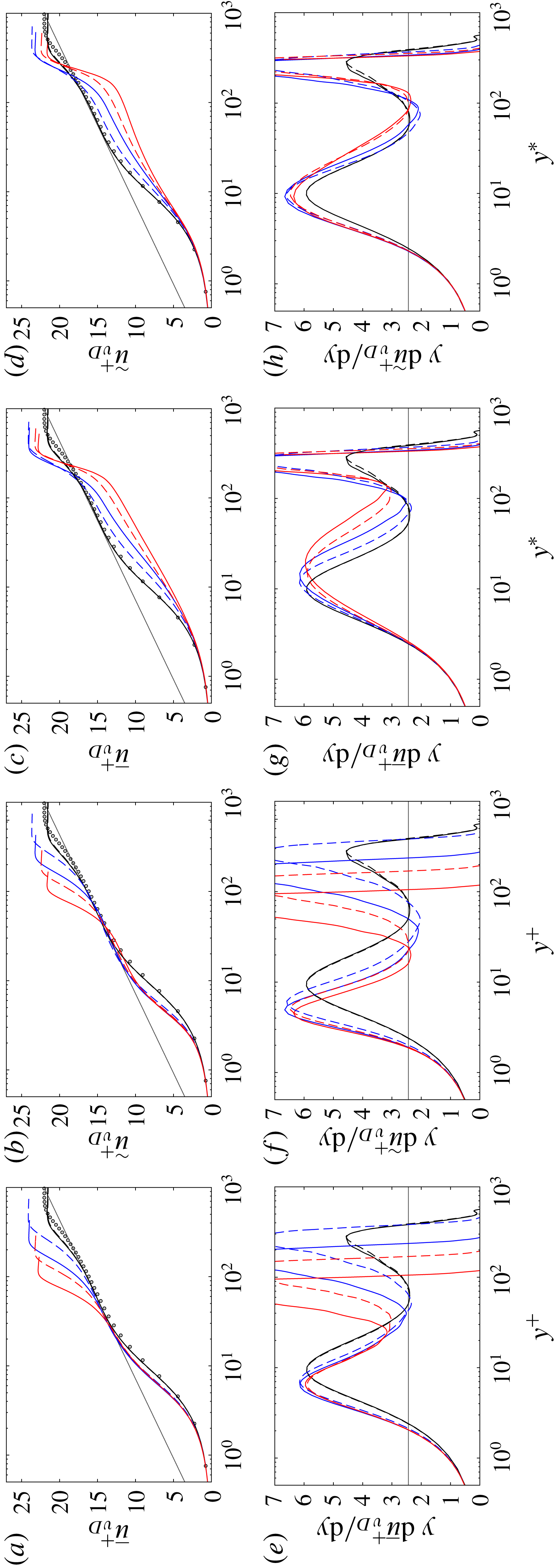
as in (3.1)), the large density fluctuations induce a distinct difference between the Reynolds- and Favre-averaged mean velocities. Figure 9 investigates how the Reynolds- and Favre-averaged mean velocities affect the van Driest transformed streamwise velocity
 $u_{vD}^{+}$
and the diagnostic function
 $y\,\text{d}u_{vD}^{+}/\text{d}y$
in the conventional inner scaling
 $y^{+}$
and the semi-local scaling
 $y^{\ast }$
. In the
 $y^{+}$
scaling (a,b), although there is a clear discrepancy between the heated transcritical and unheated non-transcritical cases, a better collapse of the heated cases in the viscous, buffer and logarithmic regions is obtained by the Reynolds-averaged velocity:
 $\overline{u}_{vD}^{+}$
in
 $y^{+}$
scaling shows a collapsed profile in the logarithmic region with the same log-law slope obtained by the incompressible perfect-gas DNS (Spalart Reference Spalart1988). However,
 $\overline{u}_{vD}^{+}$
in
 $y^{+}$
scaling with the heated wall yields a shift in the linear viscous sublayer, and for the higher wall-temperature cases the logarithmic region starts to appear in the lower
 $y^{+}$
region, as also can be seen in the diagnostic function in figure 9(e). For the unheated non-transcritical boundary layers, there is no difference between the Reynolds- and Favre-averaged mean velocities because
 $\overline{u}\approx \widetilde{u}$
, and the van Driest transformation in
 $y^{+}$
scaling closely agrees with the DNS of incompressible turbulent boundary layer by Spalart (Reference Spalart1988), indicating negligible real-fluid effects on the boundary layers when the flow temperature does not vary through the pseudo-critical temperature
 $T_{pc}$
. In the semi-local
 $y^{\ast }$
scaling (figure 9(c,d)), for the heated cases the van Driest transformed velocity clearly yields a reduced log-law additive constant and significantly deviates from the logarithmic law. As discussed in Patel et al. (Reference Patel, Boersma and Pecnik2016), when
 $\text{d}Re_{\unicode[STIX]{x1D70F}}^{\ast }/\text{d}y>0$
(see figure 4
e), the log-law additive constant as a function of
 $y^{\ast }$
is reduced. Regarding the diagnostic function, the Favre-averaged velocity (
 $\widetilde{u_{i}}=\overline{u_{i}}-\overline{u_{i}^{\prime \prime }}$
) improves the collapse of the profiles. The results indicate that the van Driest transformation fails to collapse the mean velocity to the universal law of the wall. In the following, the velocity transformation for the heated transcritical turbulent boundary layers is further investigated by introducing the streamwise stress-balance equation.
(a–d) The van Driest transformed mean streamwise velocity and (e–h) diagnostic function as a function of the inner scaling
 $y^{+}$
(a,b,e,f) and
 $y^{\ast }$
(c,d,g,h) using Reynolds- and Favre-averaged mean velocity for the heated transcritical and unheated non-transcritical turbulent boundary layers. Circles in (a–d), incompressible perfect-gas DNS by Spalart (Reference Spalart1988) at
 $Re_{\unicode[STIX]{x1D703}}=1410$
; thin grey line in (a–d),
 $u_{vD}^{+}=1/0.41\log (y^{+})+5.2$
; thin horizontal grey line in (e–h),
 $1/0.41$
. Lines as in figure 4.

By neglecting the streamwise derivatives of fluxes in the streamwise component of the mean momentum equation (the present DNS shows a negligible contribution from the streamwise derivatives of fluxes, thus validating this assumption) and integrating the equation, the streamwise stress-balance equation normalized by
 $\overline{\unicode[STIX]{x1D70F}_{w}}=\overline{\unicode[STIX]{x1D70C}}\overline{u_{\unicode[STIX]{x1D70F}}^{\ast }}^{2}$
can be written by using the semi-local scaling quantities as
 $$\begin{eqnarray}\displaystyle -\!\frac{\widetilde{u}\widetilde{v}}{\overline{u_{\unicode[STIX]{x1D70F}}^{\ast }}^{2}}-\frac{\widetilde{u^{\prime \prime }v^{\prime \prime }}}{\overline{u_{\unicode[STIX]{x1D70F}}^{\ast }}^{2}}+\frac{\unicode[STIX]{x1D6FF}}{Re_{\unicode[STIX]{x1D70F}}^{\ast }}\frac{1}{\overline{u_{\unicode[STIX]{x1D70F}}^{\ast }}}\frac{1}{\overline{\unicode[STIX]{x1D707}}}\left\{\overline{\unicode[STIX]{x1D707}\left(\frac{\unicode[STIX]{x2202}u}{\unicode[STIX]{x2202}y}+\frac{\unicode[STIX]{x2202}v}{\unicode[STIX]{x2202}x}\right)}\right\}=1, & & \displaystyle\end{eqnarray}$$
where different from the typical stress-balance equation
 $-\widetilde{u}\widetilde{v}$
is not neglected because of the non-zero near-wall
 $\widetilde{v}$
in the present heated transcritical boundary layers as shown in figure 8. Using the Reynolds- and Favre-averaging quantities, the viscous-stress term (the third term on the left-hand side of (3.2)) becomes
 $$\begin{eqnarray}\displaystyle & \displaystyle \frac{\unicode[STIX]{x1D6FF}}{Re_{\unicode[STIX]{x1D70F}}^{\ast }}\frac{1}{\overline{u_{\unicode[STIX]{x1D70F}}^{\ast }}}\frac{1}{\overline{\unicode[STIX]{x1D707}}}\left\{\overline{\unicode[STIX]{x1D707}\left(\frac{\unicode[STIX]{x2202}u}{\unicode[STIX]{x2202}y}+\frac{\unicode[STIX]{x2202}v}{\unicode[STIX]{x2202}x}\right)}\right\}=\frac{\unicode[STIX]{x1D6FF}}{Re_{\unicode[STIX]{x1D70F}}^{\ast }}\frac{1}{\overline{u_{\unicode[STIX]{x1D70F}}^{\ast }}}\left\{\frac{\unicode[STIX]{x2202}\overline{u}}{\unicode[STIX]{x2202}y}+\frac{\unicode[STIX]{x2202}\overline{v}}{\unicode[STIX]{x2202}x}+\frac{1}{\overline{\unicode[STIX]{x1D707}}}\left(\overline{\unicode[STIX]{x1D707}^{\prime }\frac{\unicode[STIX]{x2202}u^{\prime }}{\unicode[STIX]{x2202}y}}+\overline{\unicode[STIX]{x1D707}^{\prime }\frac{\unicode[STIX]{x2202}v^{\prime }}{\unicode[STIX]{x2202}x}}\right)\!\right\} & \displaystyle\end{eqnarray}$$
 $$\begin{eqnarray}\displaystyle & \displaystyle =\frac{\unicode[STIX]{x1D6FF}}{Re_{\unicode[STIX]{x1D70F}}^{\ast }}\frac{1}{\overline{u_{\unicode[STIX]{x1D70F}}^{\ast }}}\left\{\frac{\unicode[STIX]{x2202}\widetilde{u}}{\unicode[STIX]{x2202}y}+\frac{\unicode[STIX]{x2202}\widetilde{v}}{\unicode[STIX]{x2202}x}+\frac{\unicode[STIX]{x2202}\overline{u^{\prime \prime }}}{\unicode[STIX]{x2202}y}+\frac{\unicode[STIX]{x2202}\overline{v^{\prime \prime }}}{\unicode[STIX]{x2202}x}+\frac{1}{\overline{\unicode[STIX]{x1D707}}}\left(\overline{\unicode[STIX]{x1D707}^{\prime }\frac{\unicode[STIX]{x2202}u^{\prime \prime }}{\unicode[STIX]{x2202}y}}+\overline{\unicode[STIX]{x1D707}^{\prime }\frac{\unicode[STIX]{x2202}v^{\prime \prime }}{\unicode[STIX]{x2202}x}}\right)\!\right\}, & \displaystyle\end{eqnarray}$$
where
 $\overline{u_{i}^{\prime \prime }}=\overline{u_{i}}-\widetilde{u_{i}}=-\overline{\unicode[STIX]{x1D70C}^{\prime }u_{i}^{\prime }}/\overline{\unicode[STIX]{x1D70C}}$
(as in (3.1)), and
 $\overline{\unicode[STIX]{x1D707}^{\prime }\unicode[STIX]{x2202}u_{i}^{\prime }/\unicode[STIX]{x2202}x_{j}}=\overline{\unicode[STIX]{x1D707}^{\prime }\unicode[STIX]{x2202}u_{i}^{\prime \prime }/\unicode[STIX]{x2202}x_{j}}$
. If one neglects the
 $\unicode[STIX]{x2202}\overline{v}/\unicode[STIX]{x2202}x$
and
 $\unicode[STIX]{x1D707}^{\prime }$
-related terms in (3.3) (as widely employed in prior studies), the full viscous-stress terms can be reduced as
 $$\begin{eqnarray}\displaystyle \frac{\unicode[STIX]{x1D6FF}}{Re_{\unicode[STIX]{x1D70F}}^{\ast }}\frac{1}{\overline{u_{\unicode[STIX]{x1D70F}}^{\ast }}}\frac{1}{\overline{\unicode[STIX]{x1D707}}}\left\{\overline{\unicode[STIX]{x1D707}\left(\frac{\unicode[STIX]{x2202}u}{\unicode[STIX]{x2202}y}+\frac{\unicode[STIX]{x2202}v}{\unicode[STIX]{x2202}x}\right)}\right\}\approx \frac{\unicode[STIX]{x1D6FF}}{Re_{\unicode[STIX]{x1D70F}}^{\ast }}\frac{1}{\overline{u_{\unicode[STIX]{x1D70F}}^{\ast }}}\frac{\text{d}\overline{u}}{\text{d}y}=\frac{\unicode[STIX]{x1D6FF}}{Re_{\unicode[STIX]{x1D70F}}^{\ast }}\frac{\text{d}\overline{u}_{vD}^{+}}{\text{d}y}, & & \displaystyle\end{eqnarray}$$
where
 $\text{d}\overline{u}_{vD}^{+}=\sqrt{\overline{\unicode[STIX]{x1D70C}}/\overline{\unicode[STIX]{x1D70C}_{w}}}\,\text{d}(\overline{u}/\overline{u_{\unicode[STIX]{x1D70F}}})=\sqrt{\overline{\unicode[STIX]{x1D70C}}/\overline{\unicode[STIX]{x1D70C}_{w}}}\,\text{d}(\overline{u}^{+})$
(Patel et al.
Reference Patel, Peeters, Boersma and Pecnik2015). Patel et al. (Reference Patel, Boersma and Pecnik2016) found in their turbulent channel flows that the viscous stress in (3.5) plotted as a function of
 $y^{\ast }$
for different near-wall density and viscosity gradients collapses perfectly over a wide range of
 $y^{\ast }$
. Based on the universality of the viscous stress, then Patel et al. (Reference Patel, Boersma and Pecnik2016) integrate the equation (3.5) to derive the following velocity transformation:
 $$\begin{eqnarray}\displaystyle \overline{u}^{\ast }=\int _{0}^{\overline{u}_{vD}^{+}}\left(1+\frac{y}{Re_{\unicode[STIX]{x1D70F}}^{\ast }}\frac{\text{d}Re_{\unicode[STIX]{x1D70F}}^{\ast }}{\text{d}y}\right)\,\text{d}\overline{u}_{vD}^{+}. & & \displaystyle\end{eqnarray}$$
This velocity transformation as a function of semi-local wall coordinate
 $y^{\ast }$
was found to collapse mean velocity profiles to the universal law of the wall for a wide range of heated and cooled wall turbulent boundary layers with near-wall density and shear viscosity variations (Patel et al.
Reference Patel, Boersma and Pecnik2016; Trettel & Larsson Reference Trettel and Larsson2016).
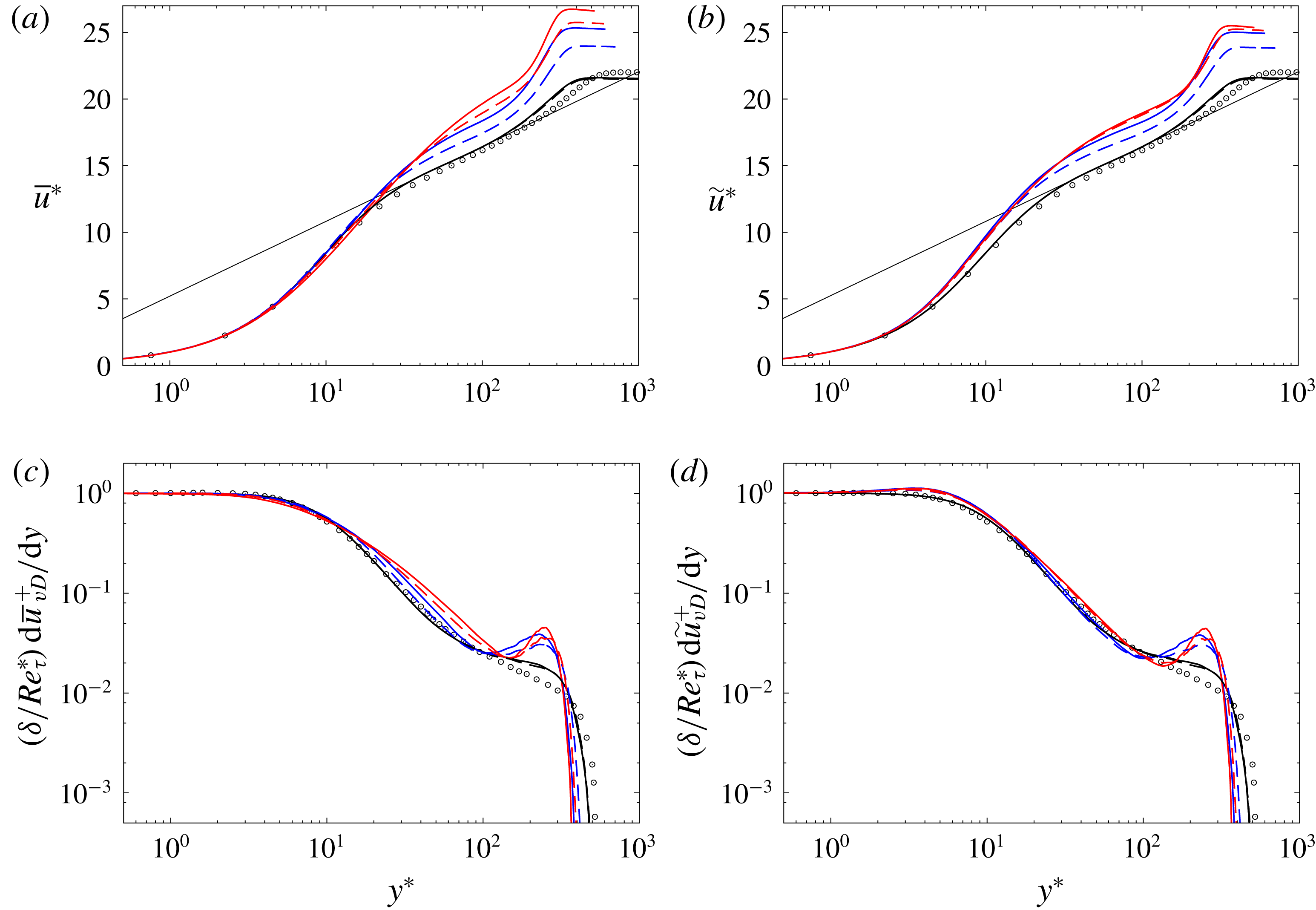
Figure 10 investigates the capability of the velocity transformation
 $u^{\ast }$
and the profiles of the viscous stress
 $(\unicode[STIX]{x1D6FF}/Re_{\unicode[STIX]{x1D70F}}^{\ast })\,\text{d}u_{vD}^{+}/\text{d}y$
as a function of
 $y^{\ast }$
using Reynolds- and Favre-averaged velocities obtained by the present study. Although a better collapse is obtained by using the Favre-averaged velocity for the heated cases (similar to the diagnostic function in figure 9), different from the findings of Patel et al. (Reference Patel, Boersma and Pecnik2016) and Trettel & Larsson (Reference Trettel and Larsson2016), the viscous stress does not collapse perfectly. The viscous stress
 $(\unicode[STIX]{x1D6FF}/Re_{\unicode[STIX]{x1D70F}}^{\ast })\,\text{d}\widetilde{u}_{vD}^{+}/\text{d}y$
obtained from the heated cases starts to deviate from the viscous and buffer profiles at
 $2\lesssim y^{\ast }\lesssim 10$
(showing a slight overshoot in
 $(\unicode[STIX]{x1D6FF}/Re_{\unicode[STIX]{x1D70F}}^{\ast })\,\text{d}\widetilde{u}_{vD}^{+}/\text{d}y$
) where the density fluctuations start to appear. Accordingly, the velocity transformation
 $\widetilde{u}^{\ast }$
also starts deviate in that region and fails to collapse the logarithmic velocity profiles to the universal law of the wall. We note that the inclusions of the
 $\unicode[STIX]{x2202}\overline{v}/\unicode[STIX]{x2202}x$
and
 $\unicode[STIX]{x1D707}^{\prime }$
-related terms as in (3.3) have a negligible impact on the viscous-stress profiles although
 $\overline{v}$
and
 $\unicode[STIX]{x1D707}^{\prime }$
are non-zero in the heated transcritical boundary layers. A significant difference between the prior studies by Patel et al. (Reference Patel, Boersma and Pecnik2016), Trettel & Larsson (Reference Trettel and Larsson2016) and the present study is the presence of significant near-wall density fluctuations
 $\sqrt{\overline{\unicode[STIX]{x1D70C}^{\prime }\unicode[STIX]{x1D70C}^{\prime }}}/\overline{\unicode[STIX]{x1D70C}}\approx 0.4{-}1.0$
that induce the non-negligible Favre-averaged velocity fluctuations
 $\overline{u_{i}^{\prime \prime }}=-\overline{\unicode[STIX]{x1D70C}^{\prime }u_{i}^{\prime }}/\overline{\unicode[STIX]{x1D70C}}$
and the near-wall wall-normal velocity as shown in figure 8. The present results indicate that a further study is needed to derive a universal inner-layer scaling law for wall-bounded flows with large near-wall density fluctuations, and this will have to be explored in future studies. Also, as expected, in the unheated non-transcritical boundary layers, both
 $u^{\ast }$
and
 $(\unicode[STIX]{x1D6FF}/Re_{\unicode[STIX]{x1D70F}}^{\ast })\,\text{d}u_{vD}^{+}/\text{d}y$
show a good collapsed profile.
(a,b) Semi-locally scaled velocity transformation
 $u^{\ast }$
and (c,d) viscous stress
 $(\unicode[STIX]{x1D6FF}/Re_{\unicode[STIX]{x1D70F}}^{\ast })\,\text{d}u_{vD}^{+}/\text{d}y$
as a function of
 $y^{\ast }$
using Reynolds- (a,c) and Favre- (b,d) averaged mean velocity for the heated transcritical and unheated non-transcritical turbulent boundary layers. Circles in (a,b) incompressible perfect-gas turbulent boundary layer DNS by Spalart (Reference Spalart1988) at
 $Re_{\unicode[STIX]{x1D703}}=1410$
; circles in (c,d) constant-property channel flow DNS by Patel et al. (Reference Patel, Boersma and Pecnik2016) at
 $Re_{\unicode[STIX]{x1D70F}}=395$
; thin grey line in (a,b),
 $u^{\ast }=1/0.41\log (y^{\ast })+5.2$
. Lines as in figure 4.

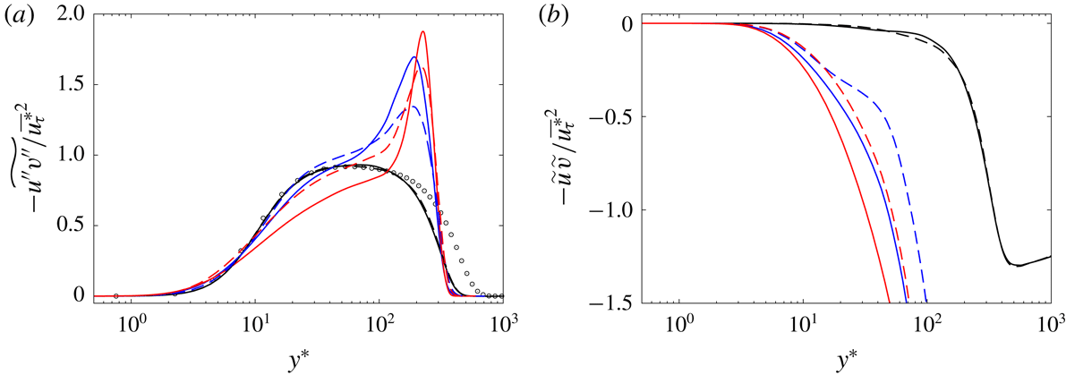
Figure 11 further investigates the streamwise stress-balance equation (3.2) by plotting the remaining two terms, the Reynolds shear stress
 $-\widetilde{u^{\prime \prime }v^{\prime \prime }}/\overline{u_{\unicode[STIX]{x1D70F}}^{\ast }}^{2}$
and the convective flux
 $-\widetilde{u}\widetilde{v}/\overline{u_{\unicode[STIX]{x1D70F}}^{\ast }}^{2}$
in the semi-local wall coordinate
 $y^{\ast }$
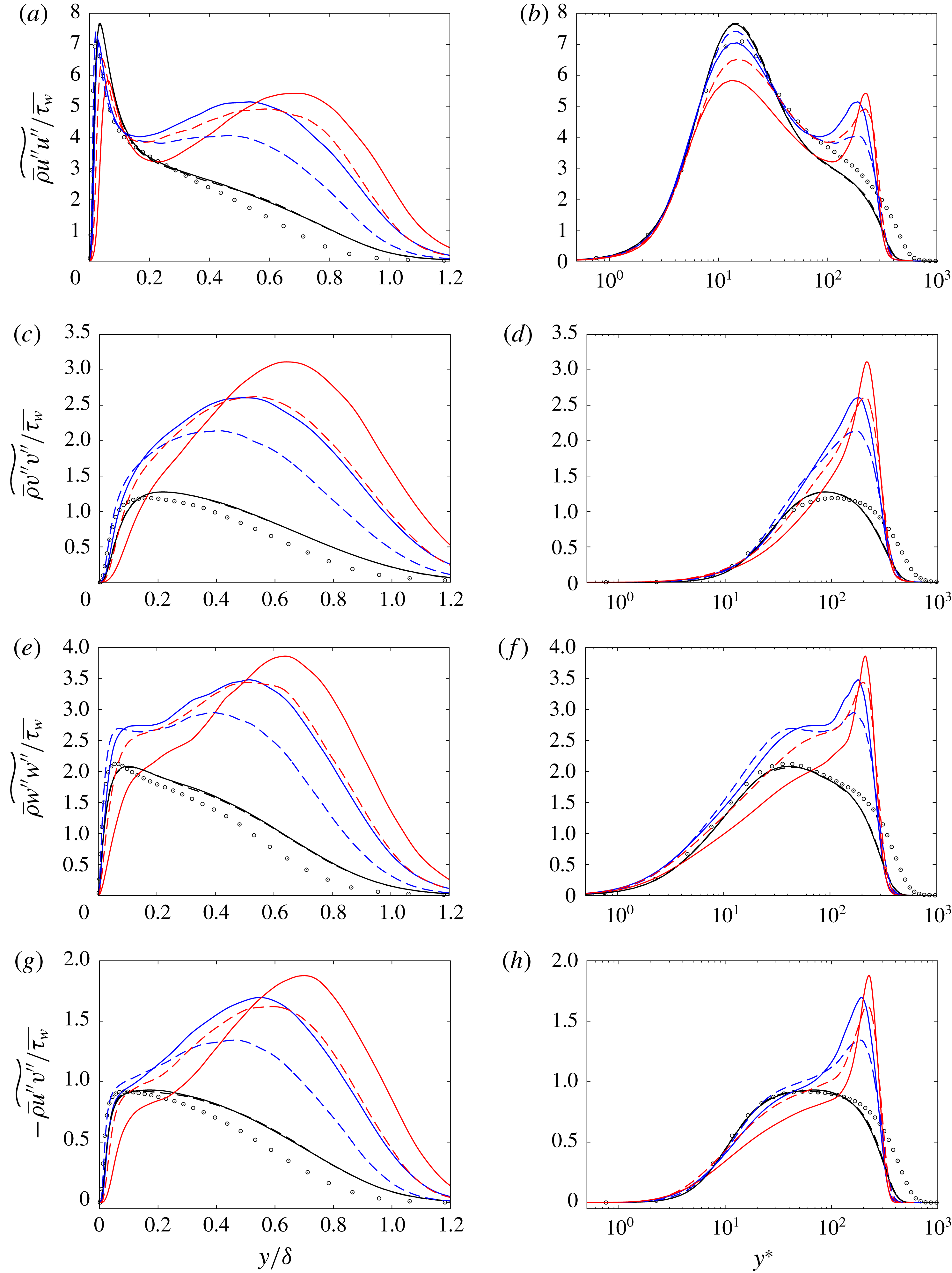
. As shown in appendix A, instead of using the conventional
 $y^{+}$
scaling, the semi-local wall coordinate
 $y^{\ast }$
improves the inner-layer scaling for the collapse of the peak locations in all the Reynolds stress components. Through the stress-balance equation in the inner layer, the shear stresses are directly connected to the logarithmic law, and Trettel & Larsson (Reference Trettel and Larsson2016) derived the velocity transformation of
 $u^{\ast }$
in (3.6) by assuming the similar profile of the Reynolds shear stress for compressible and incompressible turbulent boundary layers. As clearly seen, for the heated cases the Reynolds shear stress in the inner layer deviates from the incompressible constant-property boundary layer (Spalart Reference Spalart1988), indicating the invalidity of the assumption employed in Trettel & Larsson (Reference Trettel and Larsson2016) for heated transcritical turbulent boundary layers. This is another reason that the velocity transformation
 $u^{\ast }$
is inappropriate for the heated cases. Nevertheless, the logarithmic velocity profile in
 $u^{\ast }$
with a different log-law additive constant (and also a collapsed log-law profile of
 $\overline{u}_{vD}^{+}$
in
 $y^{+}$
scaling as shown in figure 9
a) appears in the region where the Reynolds shear stress is
 $-\widetilde{u^{\prime \prime }v^{\prime \prime }}/\overline{u_{\unicode[STIX]{x1D70F}}^{\ast }}^{2}\approx 1$
in the inner layer (although the region of
 $-\widetilde{u^{\prime \prime }v^{\prime \prime }}/\overline{u_{\unicode[STIX]{x1D70F}}^{\ast }}^{2}\approx 1$
cannot clearly be seen in the case of
 $p=2$
MPa and
 $T_{w}=200~\text{K}$
in which the
 $Re_{\unicode[STIX]{x1D70F}}$
is very small). For the unheated non-transcritical cases, the Reynolds shear stress closely agrees with the incompressible boundary layer, supporting the successful collapse of the velocity transformations
 $u^{\ast }$
and
 $u_{vD}^{+}$
for the unheated cases.
A distinct difference between the heated and unheated cases is also seen in the near-wall convective flux
 $-\widetilde{u}\widetilde{v}/\overline{u_{\unicode[STIX]{x1D70F}}^{\ast }}^{2}$
. For the heated cases,
 $-\widetilde{u}\widetilde{v}/\overline{u_{\unicode[STIX]{x1D70F}}^{\ast }}^{2}$
starts to appear near the wall at
 $y^{\ast }\gtrsim 3$
where a overshoot of the viscous stress
 $(\unicode[STIX]{x1D6FF}/Re_{\unicode[STIX]{x1D70F}}^{\ast })\,\text{d}\widetilde{u}_{vD}^{+}/\text{d}y$
appears as shown in figure 10(d), while for the unheated cases
 $-\widetilde{u}\widetilde{v}/\overline{u_{\unicode[STIX]{x1D70F}}^{\ast }}^{2}\approx 0$
throughout the inner layer (as also seen in typical turbulent boundary layers). The appearance of
 $-\widetilde{u}\widetilde{v}/\overline{u_{\unicode[STIX]{x1D70F}}^{\ast }}^{2}$
near the wall for the heated cases originates from the non-negligible mean wall-normal velocity associated with the large density fluctuations near the wall, as discussed in figure 8. The results further indicate that the significant near-wall density fluctuations alter the profiles of the total stress balance from the well-known profiles.
(a) Reynolds shear stress
 $-\widetilde{u^{\prime \prime }v^{\prime \prime }}/\overline{u_{\unicode[STIX]{x1D70F}}^{\ast }}^{2}$
and (b) convective flux
 $-\widetilde{u}\widetilde{v}/\overline{u_{\unicode[STIX]{x1D70F}}^{\ast }}^{2}$
for the heated transcritical and unheated non-transcritical turbulent boundary layers in the semi-local inner scaling
 $y^{\ast }$
. Circles in (a) show incompressible perfect-gas DNS by Spalart (Reference Spalart1988) at
 $Re_{\unicode[STIX]{x1D703}}=1410$
. Lines as in figure 4.

To investigate the effects of the density fluctuations on the Reynolds shear stress, the Reynolds shear stress is now decomposed into the mean-density-related term and density-fluctuation-related term (the first and second terms on the right-hand side of (3.7)) as follows
 $$\begin{eqnarray}\displaystyle \frac{-\widetilde{u^{\prime \prime }v^{\prime \prime }}}{\overline{u_{\unicode[STIX]{x1D70F}}^{\ast }}^{2}}=\frac{-\overline{\unicode[STIX]{x1D70C}}\widetilde{u^{\prime \prime }v^{\prime \prime }}}{\overline{\unicode[STIX]{x1D70F}_{w}}}=\frac{-\overline{\unicode[STIX]{x1D70C}}\overline{u^{\prime \prime }v^{\prime \prime }}}{\overline{\unicode[STIX]{x1D70F}_{w}}}+\frac{-\overline{\unicode[STIX]{x1D70C}^{\prime }u^{\prime \prime }v^{\prime \prime }}}{\overline{\unicode[STIX]{x1D70F}_{w}}}\left(=\frac{-\overline{u^{\prime \prime }v^{\prime \prime }}}{\overline{u_{\unicode[STIX]{x1D70F}}^{\ast }}^{2}}+\frac{-\overline{\unicode[STIX]{x1D70C}^{\prime }u^{\prime \prime }v^{\prime \prime }}}{\overline{\unicode[STIX]{x1D70C}}\overline{u_{\unicode[STIX]{x1D70F}}^{\ast }}^{2}}\right), & & \displaystyle\end{eqnarray}$$
and the contributions of each term are plotted in figure 12. For the heated transcritical cases, clearly in the inner layer the large density fluctuations (that originate from the peculiar abrupt density variations in supercritical fluids through the transcritical condition) induce a non-negligible negative contribution of the density-fluctuation-related term to the Reynolds shear stress. The approximately constant Reynolds shear stress (
 $-\widetilde{u^{\prime \prime }v^{\prime \prime }}/\overline{u_{\unicode[STIX]{x1D70F}}^{\ast }}^{2}\approx 1$
) in the inner layer where the logarithmic velocity profile in
 $u^{\ast }$
(and also
 $\overline{u}_{vD}^{+}$
) appears consists of the balance between the negative density-fluctuation-related term (
 $-\overline{\unicode[STIX]{x1D70C}^{\prime }u^{\prime \prime }v^{\prime \prime }}<0$
) and the excessive positive contribution from the mean-density-related term (
 $-\overline{\unicode[STIX]{x1D70C}}\overline{u^{\prime \prime }v^{\prime \prime }}>1$
). The results indicate that the large density fluctuations in the heated transcritical turbulent boundary layers have a non-negligible impact on the Reynolds shear stress. On the other hand, the density-fluctuation-related Reynolds shear stress is relatively small below the buffer region
 $y^{\ast }\lesssim 10$
although the density fluctuations in that region are large. The reason for this can be explained by further decomposing the Reynolds shear stress into quadrant events, as will be discussed in the following. For the unheated non-transcritical cases, since the density fluctuations are negligibly small throughout the boundary layers,
 $-\overline{\unicode[STIX]{x1D70C}^{\prime }u^{\prime \prime }v^{\prime \prime }}\approx 0$
, and thus
 $-\overline{\unicode[STIX]{x1D70C}}\widetilde{u^{\prime \prime }v^{\prime \prime }}\approx -\overline{\unicode[STIX]{x1D70C}}\overline{u^{\prime \prime }v^{\prime \prime }}$
as expected.
Decomposed mean-density-related and density-fluctuation-related Reynolds shear stresses at (a)
 $p=2$
MPa and (b) 4 MPa in the semi-local wall coordinate
 $y^{\ast }$
. Black,
 $T_{w}=T_{\infty }=25~\text{K}$
; blue,
 $T_{w}=100~\text{K}$
; red,
 $T_{w}=200~\text{K}$
; solid lines, Reynolds shear stress
 $-\overline{\unicode[STIX]{x1D70C}}\widetilde{u^{\prime \prime }v^{\prime \prime }}/\overline{\unicode[STIX]{x1D70F}_{w}}=-\widetilde{u^{\prime \prime }v^{\prime \prime }}/\overline{u_{\unicode[STIX]{x1D70F}}^{\ast }}^{2}$
; dashed lines, mean-density-related Reynolds shear stress
 $-\overline{\unicode[STIX]{x1D70C}}\overline{u^{\prime \prime }v^{\prime \prime }}/\overline{\unicode[STIX]{x1D70F}_{w}}=-\overline{u^{\prime \prime }v^{\prime \prime }}/\overline{u_{\unicode[STIX]{x1D70F}}^{\ast }}^{2}$
; dashed-dotted lines, density-fluctuation-related Reynolds shear stress
 $-\overline{\unicode[STIX]{x1D70C}^{\prime }u^{\prime \prime }v^{\prime \prime }}/\overline{\unicode[STIX]{x1D70F}_{w}}=-\overline{\unicode[STIX]{x1D70C}^{\prime }u^{\prime \prime }v^{\prime \prime }}/(\overline{\unicode[STIX]{x1D70C}}\overline{u_{\unicode[STIX]{x1D70F}}^{\ast }}^{2})$
; circles, incompressible perfect-gas DNS by Spalart (Reference Spalart1988) at
 $Re_{\unicode[STIX]{x1D703}}=1,410$
.

Quadrant analysis of the decomposed mean-density-related and density-fluctuation-related Reynolds shear stresses in the semi-local wall coordinate
 $y^{\ast }$
for the heated transcritical and unheated non-transcritical turbulent boundary layers at
 $p=2$
MPa. First quadrant Q1,
 $u^{\prime \prime }>0$
and
 $v^{\prime \prime }>0$
(right top); second quadrant Q2 (ejection),
 $u^{\prime \prime }<0$
and
 $v^{\prime \prime }>0$
(left top); third quadrant Q3,
 $u^{\prime \prime }<0$
and
 $v^{\prime \prime }<0$
(left bottom); fourth quadrant Q4 (sweep),
 $u^{\prime \prime }>0$
and
 $v^{\prime \prime }<0$
(right bottom). Lines as in figure 12.

In figure 13, the Reynolds shear stresses,
 $-\overline{\unicode[STIX]{x1D70C}}\widetilde{u^{\prime \prime }v^{\prime \prime }}$
,
 $-\overline{\unicode[STIX]{x1D70C}}\overline{u^{\prime \prime }v^{\prime \prime }}$
and
 $-\overline{\unicode[STIX]{x1D70C}^{\prime }u^{\prime \prime }v^{\prime \prime }}$
, are further decomposed into quadrant events, and the contributions to the Reynolds shear stresses from each quadrant as a function of
 $y^{\ast }$
are shown. The quadrant analysis of the Reynolds shear stresses provides detailed information on the contribution from four categories based on the velocity fluctuations (details of the analysis may be found in the recent review paper by Wallace (Reference Wallace2016)). Q1 events have
 $u^{\prime \prime }>0$
and
 $v^{\prime \prime }>0$
, Q2 events (so-called ‘ejections’) have
 $u^{\prime \prime }<0$
and
 $v^{\prime \prime }>0$
, Q3 events have
 $u^{\prime \prime }<0$
and
 $v^{\prime \prime }<0$
and Q4 events (so-called ‘sweeps’) have
 $u^{\prime \prime }>0$
and
 $v^{\prime \prime }<0$
. As will be discussed in § 4, near-wall predominant structures of streamwise low-speed (
 $u^{\prime \prime }<0$
) and high-speed (
 $u^{\prime \prime }>0$
) streaks are associated with the Q2 ejection and Q4 sweep events. Energetic Reynolds shear-stress generating events occur in the second quadrant Q2 ejection and the fourth quadrant Q4 sweep events for all the cases. In the heated transcritical boundary layers, as clearly shown, the Q2 ejection event is largely enhanced and dominates both the mean-density- and density-fluctuation-related Reynolds shear-stress generation in the inner layer. The large negative and excessive positive contributions of
 $-\overline{\unicode[STIX]{x1D70C}^{\prime }u^{\prime \prime }v^{\prime \prime }}$
and
 $-\overline{\unicode[STIX]{x1D70C}}\overline{u^{\prime \prime }v^{\prime \prime }}$
in the inner layer as discussed in figure 12 originate mainly from this Q2 ejection event, whereas the outer-layer peak of the Reynolds shear stress at
 $y^{\ast }\approx 200$
is induced by both the Q2 ejection and Q4 sweep events. Since
 $u^{\prime \prime }$
and
 $v^{\prime \prime }$
are negatively correlated in the Q2 and Q4 events,
 $-\overline{\unicode[STIX]{x1D70C}}\overline{u^{\prime \prime }v^{\prime \prime }}$
is always positive in Q2 and Q4. The large negative and a flattened positive
 $-\overline{\unicode[STIX]{x1D70C}^{\prime }u^{\prime \prime }v^{\prime \prime }}$
in the Q2 and Q4 events indicate negative and positive density fluctuations
 $\unicode[STIX]{x1D70C}^{\prime }$
in the Q2 and Q4 events. The mechanisms of density-fluctuation-related Reynolds shear-stress generation for the heated transcritical cases can be explained as follows. For the Q2 ejection event, the wall-heated high-temperature (
 $T>T_{pc}$
) gas-like low-density fluid near the wall region ejects into the low-temperature (
 $T<T_{pc}$
) high-density liquid-like fluid, and thus with this
 $\unicode[STIX]{x1D70C}^{\prime }<0$
event
 $-\overline{\unicode[STIX]{x1D70C}^{\prime }u^{\prime \prime }v^{\prime \prime }}$
becomes negative. The opposite occurs for the Q4 sweep event and
 $-\overline{\unicode[STIX]{x1D70C}^{\prime }u^{\prime \prime }v^{\prime \prime }}$
becomes positive. The Reynolds shear-stress generation mechanism in the Q2 and Q4 events for the heated transcritical boundary layers will be further discussed in detail in § 4. Also, it is now clear that a negligible
 $-\overline{\unicode[STIX]{x1D70C}^{\prime }u^{\prime \prime }v^{\prime \prime }}$
below the buffer region
 $y^{\ast }\lesssim 10$
, as shown in figure 12 for the heated cases, occurs because of the cancellation between the negative and positive
 $-\overline{\unicode[STIX]{x1D70C}^{\prime }u^{\prime \prime }v^{\prime \prime }}$
in the Q2 and Q4 events. In the quadrant Q1 and Q3 events, there is a negligible density fluctuation effect on the Reynolds shear stress, and
 $-\overline{\unicode[STIX]{x1D70C}}\widetilde{u^{\prime \prime }v^{\prime \prime }}\approx -\overline{\unicode[STIX]{x1D70C}}\overline{u^{\prime \prime }v^{\prime \prime }}$
. Although not shown here, the results of the quadrant analysis for the
 $p=4$
MPa cases are similar to the
 $p=2$
MPa cases discussed here.
Favre-averaged (a) streamwise and (b) wall-normal velocity fluctuations associated with turbulent mass flux
 $\overline{u_{i}^{\prime \prime }}=-\overline{\unicode[STIX]{x1D70C}^{\prime }u_{i}^{\prime }}/\overline{\unicode[STIX]{x1D70C}}$
in the semi-local wall coordinate
 $y^{\ast }$
for the heated transcritical and unheated non-transcritical turbulent boundary layers. Lines as in figure 4.

Quadrant analysis of Favre-averaged (a) streamwise and (b) wall-normal velocity fluctuations associated with the turbulent mass flux
 $\overline{u_{i}^{\prime \prime }}=-\overline{\unicode[STIX]{x1D70C}^{\prime }u_{i}^{\prime }}/\overline{\unicode[STIX]{x1D70C}}$
in the semi-local wall coordinate
 $y^{\ast }$
for the heated transcritical and unheated non-transcritical turbulent boundary layers. Quadrants Q1–Q4 as in figure 13. Lines as in figure 4.

Figures 14 and 15 show the Favre-averaged velocity fluctuations associated with the turbulent mass flux
 $\overline{u_{i}^{\prime \prime }}=-\overline{\unicode[STIX]{x1D70C}^{\prime }u_{i}^{\prime }}/\overline{\unicode[STIX]{x1D70C}}$
and their quadrant analysis to further illustrate the enhancement of the Q2 ejection event in the heated transcritical boundary layers. As shown in figure 14, negative and positive Favre-averaged velocity fluctuations
 $\overline{u^{\prime \prime }}$
and
 $\overline{v^{\prime \prime }}$
(and thus the positive and negative turbulent mass fluxes
 $\overline{\unicode[STIX]{x1D70C}^{\prime }u^{\prime }}$
and
 $\overline{\unicode[STIX]{x1D70C}^{\prime }v^{\prime }}$
) appear throughout the inner layer of the heated boundary layers. From the quadrant analysis of
 $\overline{u^{\prime \prime }}$
and
 $\overline{v^{\prime \prime }}$
in figure 15, in the Q2 ejection event the velocity fluctuations are clearly increased in the heated transcritical boundary layers, whereas the velocity fluctuations are decreased in the Q4 sweep event and the contributions from the Q1 and Q3 events are relatively small throughout the inner layer. The quadrant analysis indicates that the enhanced Q2 ejection event mainly contributes to the negative
 $\overline{u^{\prime \prime }}$
and positive
 $\overline{v^{\prime \prime }}$
generations as observed in figure 14. Also, the quadrant analysis identifies that the enhanced Reynolds shear stresses
 $-\overline{\unicode[STIX]{x1D70C}^{\prime }u^{\prime \prime }v^{\prime \prime }}$
and
 $-\overline{\unicode[STIX]{x1D70C}}\overline{u^{\prime \prime }v^{\prime \prime }}$
in the Q2 ejection event for the heated cases shown in figure 13 are due to the increase in the velocity fluctuations (
 $u^{\prime \prime }$
and
 $v^{\prime \prime }$
) associated with the turbulent mass flux
 $\unicode[STIX]{x1D70C}^{\prime }u_{i}^{\prime }$
in the Q2 event. The root cause of the enhanced velocity fluctuations (and associated turbulent mass flux) is the large density fluctuations induced by the peculiar pseudo-boiling phenomena at the transcritical condition, more specifically, the abrupt transition from a liquid-like high-density fluid to a gas-like low-density fluid within the narrow temperature range through the pseudo-critical temperature
 $T_{pc}$
. The mechanism of the enhanced Favre-averaged velocity fluctuations
 $u^{\prime \prime }$
and
 $v^{\prime \prime }$
and their associated turbulent mass fluxes in the Q2 ejection event will be further discussed in detail in § 4. For the unheated boundary layers, the velocity fluctuations in the Q1 and Q3 events and Q2 and Q4 events are approximately symmetric, and thus in total
 $\overline{u_{i}^{\prime \prime }}\approx 0$
throughout the boundary layers (as also seen in the evidence that
 $\overline{u_{i}}\approx \widetilde{u_{i}}$
in figure 8 and thus
 $\overline{u_{i}^{\prime \prime }}=\overline{u_{i}}-\widetilde{u_{i}}\approx 0$
).
3.3 Turbulent kinetic energy budget
In order to further investigate the heated transcritical and unheated non-transcritical turbulent boundary layers, the budget of the turbulent kinetic energy (TKE)
 $\widetilde{k}=(1/2)\widetilde{u_{i}^{\prime \prime }u_{i}^{\prime \prime }}$
is investigated in this section. The budget equation for TKE is
 $$\begin{eqnarray}\displaystyle \left.\begin{array}{@{}c@{}}\displaystyle \frac{\unicode[STIX]{x2202}\overline{\unicode[STIX]{x1D70C}}\widetilde{k}}{\unicode[STIX]{x2202}t}=-C+P+T_{d}+T_{p}+D_{v}+D_{d}+M+\unicode[STIX]{x1D6F1}_{d},\\ \displaystyle C=\frac{\unicode[STIX]{x2202}}{\unicode[STIX]{x2202}x_{j}}\left(\overline{\unicode[STIX]{x1D70C}}\widetilde{u_{j}}\widetilde{k}\right),\quad P=-\overline{\unicode[STIX]{x1D70C}}\widetilde{u_{i}^{\prime \prime }u_{i}^{\prime \prime }}\frac{\unicode[STIX]{x2202}\widetilde{u_{i}}}{\unicode[STIX]{x2202}x_{j}},\\ \displaystyle T_{d}=-\frac{\unicode[STIX]{x2202}}{\unicode[STIX]{x2202}x_{j}}\left(\frac{1}{2}\overline{\unicode[STIX]{x1D70C}}\widetilde{u_{i}^{\prime \prime }u_{i}^{\prime \prime }u_{j}^{\prime \prime }}\right),\quad T_{p}=-\frac{\unicode[STIX]{x2202}}{\unicode[STIX]{x2202}x_{j}}\left(\overline{p^{\prime }u_{j}^{\prime }}\right),\\ \displaystyle D_{v}=\frac{\unicode[STIX]{x2202}}{\unicode[STIX]{x2202}x_{j}}\left(\overline{\unicode[STIX]{x1D70F}_{ij}^{\prime }u_{i}^{\prime }}\right),\quad D_{d}=-\overline{\unicode[STIX]{x1D70F}_{ij}^{\prime }\frac{\unicode[STIX]{x2202}u_{i}^{\prime }}{\unicode[STIX]{x2202}x_{j}}},\quad M=\overline{u_{i}^{\prime \prime }}\left(\frac{\unicode[STIX]{x2202}\overline{\unicode[STIX]{x1D70F}_{ij}}}{\unicode[STIX]{x2202}x_{j}}-\frac{\unicode[STIX]{x2202}\overline{p}}{\unicode[STIX]{x2202}x_{i}}\right),\quad \unicode[STIX]{x1D6F1}_{d}=\overline{p^{\prime }\frac{\unicode[STIX]{x2202}u_{i}^{\prime }}{\unicode[STIX]{x2202}x_{i}}},\end{array}\right\} & & \displaystyle\end{eqnarray}$$
where
 $C$
,
 $P$
,
 $T_{d}$
,
 $T_{p}$
,
 $D_{v}$
,
 $D_{d}$
,
 $M$
and
 $\unicode[STIX]{x1D6F1}_{d}$
are the contributions from the convection, production, turbulent diffusion, velocity–pressure interaction, viscous diffusion, energy dissipation, mass flux contribution associated with density fluctuations and pressure dilatation, respectively. The mass flux contribution
 $M$
and pressure-dilatation term
 $\unicode[STIX]{x1D6F1}_{d}$
originate from the compressibility effects and are basically negligible in incompressible flows.
Turbulent kinetic energy budget normalized by the semi-local scaling
 $\overline{\unicode[STIX]{x1D70F}_{w}}^{2}/\overline{\unicode[STIX]{x1D707}}$
in the semi-local wall coordinate
 $y^{\ast }$
obtained by (a,b) unheated non-transcritical turbulent boundary layers with
 $T_{w}=25~\text{K}$
and (c–f) heated transcritical turbulent boundary layers with (c,d)
 $T_{w}=100~\text{K}$
and (e,f)
 $T_{w}=200~\text{K}$
at
 $p=2$
MPa (a,c,e) and 4 MPa (b,d,f). Black, convection
 $C$
; blue, production
 $P$
; orange, turbulent diffusion
 $T_{d}$
; purple, velocity–pressure interaction
 $T_{p}$
; dark green, viscous diffusion
 $D_{v}$
; light green, energy dissipation
 $D_{d}$
; red, mass flux contribution
 $M$
; cyan, pressure dilatation
 $\unicode[STIX]{x1D6F1}_{d}$
. Symbols (circles,
 $P$
; triangles,
 $T_{d}$
; crosses,
 $T_{p}$
; squares,
 $D_{v}$
; pluses,
 $D_{d}$
), incompressible perfect-gas DNS by Spalart (Reference Spalart1988) at
 $Re_{\unicode[STIX]{x1D703}}=1410$
.

All the terms in the TKE budget equation near the wall obtained by the heated transcritical and unheated non-transcritical boundary layers are shown in figure 16. Here the budget terms are normalized by the semi-local scaling of
 $\overline{\unicode[STIX]{x1D70F}_{w}}^{2}/\overline{\unicode[STIX]{x1D707}}$
proposed by Foysi, Sarkar & Friedrich (Reference Foysi, Sarkar and Friedrich2004) and plotted in the semi-local inner-layer wall coordinate
 $y^{\ast }$
. Although not shown here, the semi-local scaling
 $\overline{\unicode[STIX]{x1D70F}_{w}}^{2}/\overline{\unicode[STIX]{x1D707}}$
improves the collapse in terms of the amplitude of the incompressible turbulent boundary layer, especially for the production term, compared to the conventional scaling
 $\overline{\unicode[STIX]{x1D70C}_{w}}\overline{u_{\unicode[STIX]{x1D70F}}}^{4}/\overline{\unicode[STIX]{x1D708}_{w}}=\overline{\unicode[STIX]{x1D70F}_{w}}^{2}/\overline{\unicode[STIX]{x1D707}_{w}}$
used in the incompressible constant-property situation. Regarding the inner-layer wall coordinate, the semi-local inner-layer scaling
 $y^{\ast }$
improves the collapse of the peak location for each term compared to the conventional
 $y^{+}$
scaling. In the unheated non-transcritical boundary layers, similar to the mean velocity and Reynolds shear stress, as expected, all the budget terms agree well with the incompressible perfect-gas turbulent boundary layer by Spalart (Reference Spalart1988), indicating additional evidence of a negligible contribution of the real-fluid effects. The contributions of the convection term
 $C$
and the compressibility effects (i.e.
 $M$
and
 $\unicode[STIX]{x1D6F1}_{d}$
) are approximately zero throughout the boundary layers. The contributions of the budget terms are altered in the heated transcritical boundary layers and the discrepancies from the TKE budget obtained by the unheated non-transcritical boundary layers (and also the incompressible boundary layers) become noticeable. The mass flux contribution
 $M$
is now noticeable as one of the main positive terms, and the peak location appears around
 $y^{\ast }\approx 10$
, similar to the production peak where the large density fluctuations are generated. As in (3.8), the mass flux contribution term
 $M$
contains
 $\overline{u_{i}^{\prime \prime }}$
that is associated with the turbulent mass flux through
 $\overline{u_{i}^{\prime \prime }}=-\overline{\unicode[STIX]{x1D70C}^{\prime }u_{i}^{\prime }}/\overline{\unicode[STIX]{x1D70C}}$
(equation (3.1)), and thus the appearance of
 $M$
in the heated cases is induced by the large density fluctuations. Also, different from the unheated non-transcritical boundary layers, the convection
 $C$
and pressure-dilatation
 $\unicode[STIX]{x1D6F1}_{d}$
terms are non-zero near the wall (although the contributions are relatively small). The non-zero
 $C$
and
 $\unicode[STIX]{x1D6F1}_{d}$
originate from the non-negligible
 $\widetilde{v}$
and the appearance of flow expansion and compression due to the abrupt density variations through the transcritical region (the mechanism of the flow expansion and compression will be discussed in § 4). By considering the local variations in
 $\overline{\unicode[STIX]{x1D707}}$
for the semi-local scaling
 $\overline{\unicode[STIX]{x1D70F}_{w}}^{2}/\overline{\unicode[STIX]{x1D707}}$
as proposed by Foysi et al. (Reference Foysi, Sarkar and Friedrich2004), the production term
 $P$
closely agrees with the incompressible boundary layer except the heated case with the highest density fluctuations (
 $p=2$
MPa and
 $T_{w}=200~\text{K}$
case) where the peak production value is reduced. The remaining budget terms in the heated transcritical cases show a partial success of the collapse, whereas a deviation is seen in the region where the density fluctuations are large, suggesting a certain effect of the density fluctuations on the other budget terms as well.
The results indicate that the large density fluctuations that are induced by the peculiar abrupt density variations at the transcritical condition (i.e. the pseudo-boiling process) alter the balance of the TKE budget equation. Especially, the appearance of the compressibility term, more specifically, the mass flux contribution term
 $M$
associated with the density fluctuations, is noticeable in the heated transcritical boundary layers.
4 Near-wall turbulent structures
Instantaneous wall-parallel (
 $x$
–
 $z$
plane) snapshots of the heated transcritical turbulent boundary layer at
 $y^{\ast }\approx 19.5$
in the region of
 $0\leqslant x/\unicode[STIX]{x1D6FF}_{0}\leqslant 30$
and
 $0\leqslant z/\unicode[STIX]{x1D6FF}_{0}\leqslant 6$
(whole right-side domain in figure 2) on the left and the zoomed region (black box region in a) with superimposed black contour lines of high
 $c_{p}$
regions on the right at
 $p=2$
MPa and
 $T_{w}=100$
K condition. (a) Temperature, (b) specific heat at constant pressure, (c) density fluctuations, (d) Favre-averaged streamwise velocity fluctuations, (e) Favre-averaged wall-normal velocity fluctuations, (f) divergence of velocity fluctuations.

Figure 17 shows instantaneous snapshots of the wall-parallel plane at
 $y^{\ast }\approx 19.5$
for the heated transcritical boundary layer at the
 $p=2$
MPa and
 $T_{w}=100$
K condition. Around
 $y^{\ast }\approx 19.5$
, the density fluctuations reach its maximum, and the Favre-averaged velocity fluctuations are enhanced in the Q2 ejection event. The region of the square box with black line (only shown in figure 17
a) is zoomed in and shown with the superimposed black contour lines of high
 $c_{p}$
regions on the right. Since
 $c_{p}$
reaches its maximum value at
 $T=T_{pc}$
, the filaments of high
 $c_{p}$
regions indicate the instantaneous transcritical regions (
 $T\approx T_{pc}$
) where the pseudo-boiling phenomena occur. As seen in figure 17(d), typical streamwise-elongated narrow low-speed (blue-coloured
 $u^{\prime \prime }<0$
regions) and high-speed (red- and yellow-coloured
 $u^{\prime \prime }>0$
regions) streaks are observed in the near-wall region. The low-speed streaks are accompanied by the upward (
 $v^{\prime \prime }>0$
) vertical transport of the near-wall low-speed and heated gas-like-low-density fluid (
 $T>T_{pc}$
), and thus contribute to the Q2 ejection event with the properties of
 $u^{\prime \prime }<0$
,
 $v^{\prime \prime }>0$
, and
 $\unicode[STIX]{x1D70C}^{\prime }<0$
as clearly seen in the zoomed-in figures. The high-speed streaks are accompanied by the downward (
 $v^{\prime \prime }<0$
) vertical transport of the upper-portion high-speed and unheated liquid-like high-density fluid (
 $T<T_{pc}$
), and contribute to the Q4 sweep event with the properties of
 $u^{\prime \prime }>0$
,
 $v^{\prime \prime }<0$
and
 $\unicode[STIX]{x1D70C}^{\prime }>0$
. Similar to the incompressible constant-property turbulent boundary layers (e.g. Kline et al.
Reference Kline, Reynolds, Schraub and Runstadler1967; Kim, Kline & Reynolds Reference Kim, Kline and Reynolds1971), the streaky low-speed and high-speed wall-layer structures with Q2 ejection and Q4 sweep dominate the Reynolds shear-stress generation (and also the production of turbulent kinetic energy) for the present heated transcritical turbulent boundary layers. However, as discussed in figures 13 and 15, different from the conventional boundary layers, the Favre-averaged velocity fluctuations
 $u^{\prime \prime }$
and
 $v^{\prime \prime }$
and the resultant Reynolds shear stress are enhanced in the Q2 ejection event and reduced in the Q4 sweep event. In this section, we further elucidate the mechanisms associated with the density fluctuations and the resultant turbulence statistics discussed in § 3 by looking into the instantaneous near-wall turbulent structures.
As seen in figure 17(c–e), when the flow is heated by the high-temperature wall in the region
 $x>5\unicode[STIX]{x1D6FF}_{0}$
, the large density fluctuations start to be generated, and the Favre-averaged velocity fluctuations in the low-speed streaks associated with the Q2 ejection are enhanced. The instantaneous Favre-averaged velocity fluctuations can be written as
 $$\begin{eqnarray}\displaystyle u_{i}^{\prime \prime }=u-\widetilde{u}=u_{i}^{\prime }-\frac{\overline{\unicode[STIX]{x1D70C}^{\prime }u_{i}^{\prime }}}{\overline{\unicode[STIX]{x1D70C}}}. & & \displaystyle\end{eqnarray}$$
In low-speed streaks associated with the Q2 ejection, the near-wall heated low-density fluid is lifted up and thus
 $\unicode[STIX]{x1D70C}^{\prime }<0$
. Because of the correlation between
 $\unicode[STIX]{x1D70C}^{\prime }$
and
 $u_{i}^{\prime }$
, the positive streamwise and negative wall-normal turbulent mass fluxes (i.e.
 $\unicode[STIX]{x1D70C}^{\prime }u^{\prime }>0$
and
 $\unicode[STIX]{x1D70C}^{\prime }v^{\prime }<0$
) are induced in the low-speed streaks. According to (4.1), these turbulent mass fluxes enhance the negative and positive Favre-averaged instantaneous velocity fluctuations
 $u^{\prime \prime }$
and
 $v^{\prime \prime }$
in the low-speed streaks. This enhancement of the velocity fluctuations in the Q2 ejection along the low-speed streaks results in the statistics of the increased negative
 $\overline{u^{\prime \prime }}$
and positive
 $\overline{v^{\prime \prime }}$
in the Q2 ejection as shown in figure 15. On the other hand, the Favre-averaged velocity fluctuations in the Q4 sweep event (
 $u^{\prime \prime }>0$
and
 $v^{\prime \prime }<0$
) associated with the high-speed streaks are reduced. The high-speed streaks consist of the low-temperature and high-density fluid from the upper portion of the boundary layer and thus are accompanied by
 $\unicode[STIX]{x1D70C}^{\prime }>0$
. In the high-speed streaks, because of
 $\unicode[STIX]{x1D70C}^{\prime }>0$
, the turbulent mass fluxes become
 $\unicode[STIX]{x1D70C}^{\prime }u^{\prime }>0$
and
 $\unicode[STIX]{x1D70C}^{\prime }v^{\prime }<0$
. Therefore, the turbulent mass fluxes act to reduce the instantaneous velocity fluctuations
 $u^{\prime \prime }$
and
 $v^{\prime \prime }$
, resulting in the reduced
 $\overline{u^{\prime \prime }}$
and
 $\overline{v^{\prime \prime }}$
in the inner layer of the Q4 sweep event as shown in figure 15.
In the heated wall region, the divergence of the velocity fluctuations
 $\unicode[STIX]{x2202}u_{i}^{\prime }/\unicode[STIX]{x2202}x_{i}$
starts to appear along the high
 $c_{p}$
filaments. The divergence of the velocity fluctuations consists of a pair of expansion (positive divergence) and compression (negative divergence) layers. The mechanism of the divergence of the velocity fluctuations can be interpreted as follows: around the high
 $c_{p}$
filaments, the low-temperature high-density liquid-like fluid (which is associated with the high-speed streaks) is heated by the surrounding high-temperature fluid, and the fluid temperature varies through
 $T_{pc}$
. The opposite occurs for the high-temperature low-density gas-like fluid of the low-speed streaks. In these regions, because of the peculiar abrupt density variations through the transcritical condition, the local flow density varies abruptly along the temperature–density diagram, as shown in figure 1(a). Considering the mass conservation, the flow expands rapidly (i.e. showing positive divergence) when the low-temperature fluid is heated and the density decreases abruptly. Also, with the same reasoning, a compression appears when the high-temperature fluid is cooled by the surrounding low-temperature fluid. These expansion and compression processes are considered to occur rapidly within a narrow temperature range across the transcritical condition and thus appear side by side as seen in figure 17(f). The appearance of the non-zero pressure-dilatation term
 $\unicode[STIX]{x1D6F1}_{d}$
in the TKE budget originates from these phenomena.
To investigate the mechanisms of the Reynolds shear-stress generation in the Q2 ejection and Q4 sweep events, figure 18 shows the instantaneous cross-view flow fields obtained by the heated transcritical boundary layer at
 $x=25\unicode[STIX]{x1D6FF}_{0}$
at the same instant in figure 17. Generally speaking, the regions of the convex high
 $c_{p}$
filament correspond to the heated high-temperature and low-density (i.e.
 $\unicode[STIX]{x1D70C}^{\prime }<0$
) low-speed streaks associated with the Q2 ejection (
 $u^{\prime \prime }<0$
and
 $v^{\prime \prime }>0$
), and the concave regions are the low-temperature and high-density (i.e.
 $\unicode[STIX]{x1D70C}^{\prime }>0$
) high-speed streaks associated with the Q4 sweep (
 $u^{\prime \prime }>0$
and
 $v^{\prime \prime }<0$
). The interactions between these near-wall predominant streak structures and the density variations through the transcritical condition cause the Reynolds shear-stress generation shown in figure 13. In the low-speed streaks (Q2 ejection event),
 $u^{\prime \prime }<0$
,
 $v^{\prime \prime }>0$
and
 $\unicode[STIX]{x1D70C}^{\prime }<0$
, and thus
 $-\unicode[STIX]{x1D70C}^{\prime }u^{\prime \prime }v^{\prime \prime }<0$
and
 $-\overline{\unicode[STIX]{x1D70C}}u^{\prime \prime }v^{\prime \prime }>0$
. In the high-speed streaks (Q4 ejection event),
 $u^{\prime \prime }>0$
,
 $v^{\prime \prime }<0$
and
 $\unicode[STIX]{x1D70C}^{\prime }>0$
, and thus
 $-\unicode[STIX]{x1D70C}^{\prime }u^{\prime \prime }v^{\prime \prime }>0$
and
 $-\overline{\unicode[STIX]{x1D70C}}u^{\prime \prime }v^{\prime \prime }>0$
. These features are consistent to the statistical observations in figure 13. Similarly, the turbulent mass fluxes are
 $\unicode[STIX]{x1D70C}^{\prime }u^{\prime }>0$
and
 $\unicode[STIX]{x1D70C}^{\prime }v^{\prime }<0$
in both the low-speed and high-speed streaks as shown in figure 18(g,h). Although the near-wall streak structures with the density fluctuations cause the Reynolds shear-stress generation, similar to the observations in the wall-parallel plane, the enhancements of the instantaneous Favre-averaged velocity fluctuations
 $u^{\prime \prime }$
and
 $v^{\prime \prime }$
(that are the components of the Reynolds shear stress) and the turbulent mass fluxes are clearly observed in the low-speed streak regions associated with the Q2 ejection as shown in figure 18(e–h). As discussed in (4.1), the velocity fluctuations and turbulent mass flux are closely related to each other
 $u_{i}^{\prime \prime }=u_{i}^{\prime }-\overline{\unicode[STIX]{x1D70C}^{\prime }u_{i}^{\prime }}/\overline{\unicode[STIX]{x1D70C}}$
(and thus
 $\overline{u_{i}^{\prime \prime }}=-\overline{\unicode[STIX]{x1D70C}^{\prime }u_{i}^{\prime }}/\overline{\unicode[STIX]{x1D70C}}$
as in (3.1)), and thus the enhanced positive and negative turbulent mass fluxes
 $\unicode[STIX]{x1D70C}^{\prime }u^{\prime }$
and
 $\unicode[STIX]{x1D70C}^{\prime }v^{\prime }$
amplify the negative and positive instantaneous Favre-averaged velocity fluctuations of
 $u^{\prime \prime }$
and
 $v^{\prime \prime }$
in the low-speed streaks. On the other hand, the positive and negative turbulent mass fluxes reduce the velocity fluctuations in the high-speed streaks. The enhanced and reduced Reynolds shear stresses (
 $-\overline{\unicode[STIX]{x1D70C}^{\prime }u^{\prime \prime }v^{\prime \prime }}$
and
 $-\overline{\unicode[STIX]{x1D70C}}\overline{u^{\prime \prime }v^{\prime \prime }}$
) and the velocity fluctuations in the Q2 ejection and Q4 sweep events are caused by this mechanism. Also, it is now clear that the pair of intensive expansion and compression are mainly generated near the wall regions
 $y^{\ast }\lesssim 50$
where the large density fluctuations are induced. The appearance of all these density-fluctuation-related flow quantities originates from the interactions between the near-wall turbulence and the peculiar density variations through the transcritical condition. Although not shown here, in the unheated non-transcritical boundary layers, all the density-fluctuation-related flow quantities are negligibly small throughout the boundary layers.
Instantaneous cross-view (
 $y$
–
 $z$
plane) snapshots of the heated transcritical turbulent boundary layer (
 $p=2$
MPa and
 $T_{w}=100$
K) at
 $x=25\unicode[STIX]{x1D6FF}_{0}$
in the region of
 $0\leqslant y/\unicode[STIX]{x1D6FF}_{0}\leqslant 1.5$
and
 $0\leqslant z/\unicode[STIX]{x1D6FF}_{0}\leqslant 6$
with superimposed black contour lines of filaments of high
 $c_{p}$
regions at the same instant in figure 17. (a) Temperature (K), (b) specific heat at constant pressure (J/kg/K), (c) density fluctuations, (d) divergence of velocity fluctuations, (e) Favre-averaged streamwise velocity fluctuations, (f) Favre-averaged wall-normal velocity fluctuations, (g) streamwise turbulent mass flux:
 $\unicode[STIX]{x1D70C}^{\prime }u^{\prime }/(\overline{\unicode[STIX]{x1D70C}}u_{\infty })$
, (h) wall-normal turbulent mass flux:
 $\unicode[STIX]{x1D70C}^{\prime }v^{\prime }/(\overline{\unicode[STIX]{x1D70C}}u_{\infty })$
.

Isosurfaces of near-wall (a) low-speed (
 $u^{\prime \prime }/u_{\infty }=-0.12$
) and (b) high-speed (
 $u^{\prime \prime }/u_{\infty }=0.08$
) streaks in the heated transcritical turbulent boundary layer (
 $p=2$
MPa and
 $T_{w}=100$
K) coloured by density fluctuations at the same instant in figure 17. Grey coloured contours are the specific heat at constant pressure (the dark colour indicates high
 $c_{p}$
regions) at four cross-view (
 $y$
–
 $z$
) planes at
 $x/\unicode[STIX]{x1D6FF}_{0}=15$
, 20, 25, 30 and at the wall-parallel plane at
 $y^{\ast }\approx 19.5$
.

Three-dimensional structures of the near-wall low-speed and high-speed streaks are visualized and coloured by the density fluctuations in figure 19. The grey-coloured contours are the specific heat at constant pressure and the dark colour indicates high
 $c_{p}$
transcritical regions. The low-speed streaks show longitudinal structures with negative density fluctuations and are located within the convex high
 $c_{p}$
regions. The high-speed streaks accompanied by the positive density fluctuations do not show clear longitudinal structures and appear around the regions surrounded by the high
 $c_{p}$
filaments, as shown in the wall-parallel plane. Since the semi-local viscous length scale (i.e. semi-local wall units) remains largely unchanged in the region
 $15\leqslant x/\unicode[STIX]{x1D6FF}_{0}\leqslant 30$
, the characteristic dimensions of the streaks also remain almost unchanged in the flow direction.
5 Summary and conclusions
Nominally zero-pressure-gradient fully developed flat-plate turbulent boundary layers with heated and unheated isothermal walls at supercritical pressures have been studied by solving the full compressible Navier–Stokes equations using direct numerical simulation (DNS). The primary objective of this study is to investigate the influence of the strongly nonlinear real-fluid effects induced by the pseudo-boiling process at the transcritical condition on near-wall turbulence and the resultant turbulence statistics. The pseudo-boiling phenomena induce abrupt variations in thermodynamic and fluid transport properties within a narrow temperature range through the pseudo-critical temperature
 $T_{pc}$
. In this study, to investigate the effects of the peculiar behaviours of the variable properties at the transcritical condition, the heated isothermal wall temperature is set such that the flow temperature varies through the pseudo-critical temperature within the boundary layers.
In the present study, a noticeable key difference from the prior studies of turbulent boundary layers at supercritical pressure (and also turbulent boundary layers with variable thermodynamic and fluid transport properties) appears in the density fluctuations. Because of the pseudo-boiling phenomena, i.e. more specifically, the abrupt density variations through the transcritical condition, the large density fluctuations
 $\sqrt{\overline{\unicode[STIX]{x1D70C}^{\prime }\unicode[STIX]{x1D70C}^{\prime }}}/\overline{\unicode[STIX]{x1D70C}}\approx 0.4{-}1.0$
are induced within the heated transcritical turbulent boundary layers, and the large density fluctuations are found to significantly alter the near-wall turbulence and the resultant turbulence statistics.
It was found that the large density fluctuations appeared in the heated transcritical boundary layers induce non-negligible turbulent mass flux
 $\unicode[STIX]{x1D70C}^{\prime }u_{i}^{\prime }$
in the inner layer and the turbulent mass flux amplifies the Favre-averaged velocity fluctuations
 $u_{i}^{\prime \prime }$
in the near-wall low-speed streaks associated with the ejection, while reducing the Favre-averaged velocity fluctuations in the high-speed streaks associated with the sweep. Because of the peculiar abrupt density variations through the transcritical condition, the low-speed streaks consist of the wall-heated high-temperature (
 $T>T_{pc}$
) and gas-like low-density fluid (and thus
 $\unicode[STIX]{x1D70C}^{\prime }<0$
), and the high-speed streaks are low-temperature and liquid-like high-density fluid (
 $\unicode[STIX]{x1D70C}^{\prime }>0$
). Although the near-wall low-speed and high-speed streak structures dominate the Reynolds shear-stress generation, we find that the energized velocity fluctuations in the low-speed streaks enhance both the mean-density- and density-fluctuation-related Reynolds shear stresses in the ejection event, while reducing the Reynolds shear stresses in the high-speed streaks (sweep event). These changes in the Reynolds shear stresses alter the Reynolds shear-stress profile from the well-known profile of incompressible constant-property turbulent boundary layers. The large density fluctuations also alter the near-wall viscous-stress profile and induce the near-wall convective flux
 $-\overline{\unicode[STIX]{x1D70C}}\widetilde{u}\widetilde{v}$
(due to the non-zero
 $\widetilde{v}$
) in the streamwise stress-balance equation. Because of the changes in each term in the stress-balance equation, it was found that the existing velocity transformations (Van Driest Reference Van Driest1951; Patel et al.
Reference Patel, Boersma and Pecnik2016; Trettel & Larsson Reference Trettel and Larsson2016) fail to collapse the logarithmic velocity profiles to the universal law of the wall. The present results indicate that a further study is needed to derive a universal inner-layer scaling law for the turbulent boundary layer with large near-wall density fluctuations.
The large density fluctuations also greatly contribute to the turbulent kinetic energy budget. The density fluctuations directly cause the appearance of the mass flux contribution term associated with the turbulent mass flux as one of the main positive terms. The large density fluctuations also induce the flow expansion and compression, leading non-zero pressure-dilatation term (although the contribution is small). The semi-local scaling that accounts for the local variations of the mean shear viscosity proposed by Foysi et al. (Reference Foysi, Sarkar and Friedrich2004) plotted in the semi-local inner-layer wall coordinate improves the collapse of each budget term although the collapse is not perfect.
The turbulence statistics obtained by the unheated non-transcritical turbulent boundary layers (in which the flow temperature does not vary through the pseudo-critical temperature) were found to agree well with the results obtained by incompressible constant-property turbulent boundary layers. This agreement is due to the negligible property variations and dilatation
 $\unicode[STIX]{x2202}u_{i}^{\prime }/\unicode[STIX]{x2202}x_{i}$
throughout the boundary layers. The result suggests that a distinct feature in turbulent boundary layers at supercritical pressure appears when pseudo-boiling phenomena occur (i.e. liquid-like and gas-like fluids co-exist) within the boundary layer, which induces the strong variations in the mean and variances of variable properties.
Although the full compressible Navier–Stokes equations are solved in the present study, the low Mach number assumption of the compressible Navier–Stokes equations was widely used in prior studies. In the low Mach number assumption, the density (and also fluid transport properties) is approximated as a function of
 $\unicode[STIX]{x1D70C}=f(T,\overline{p})$
, independent of pressure fluctuations (Nemati et al.
Reference Nemati, Patel, Boersma and Pecnik2015; Patel et al.
Reference Patel, Boersma and Pecnik2016). Therefore, this suggests that the low Mach number formulation could involve errors associated with
 $p^{\prime }$
especially at the transcritical condition (i.e. it may be considered that the density fluctuations that were found to have an important effect on the turbulent boundary layers could potentially be underestimated).
Acknowledgements
This work was supported by the Japan Society for the Promotion of Science (JSPS) Grant-in-Aid for Young Scientists (A) KAKENHI 26709066. Computer resources of the K computer were provided by the RIKEN Advanced Institute for Computational Science through the HPCI System Research project (project ID: hp150035, hp160133, and hp170056). The author is grateful to Dr H. Abe, Dr H. Terashima and Mr Y. Miyazawa for valuable discussions. The author also gratefully acknowledges the referees for insightful comments.
Appendix A. Mean variable properties and Reynolds stresses
The mean specific heat at constant pressure, thermal conductivity, speed of sound and turbulent Prandtl number within the boundary layers are shown in figure 20 where the turbulent Prandtl number
 $Pr_{t}$
is defined as (Pirozzoli, Grasso & Gatski Reference Pirozzoli, Grasso and Gatski2004)
 $$\begin{eqnarray}\displaystyle Pr_{t}=\frac{-\overline{\unicode[STIX]{x1D70C}}\widetilde{u^{\prime \prime }v^{\prime \prime }}\left/{\displaystyle \frac{\text{d}\widetilde{u}}{\text{d}y}}\right.}{-\overline{\unicode[STIX]{x1D70C}}\widetilde{v^{\prime \prime }T^{\prime \prime }}\left/{\displaystyle \frac{\text{d}\widetilde{T}}{\text{d}y}}\right.}. & & \displaystyle\end{eqnarray}$$
Corresponding to the location where the mean temperature varies through
 $T_{pc}$
, the specific heat at constant pressure
 $\overline{c_{p}}$
reaches approximately its maximum value. According to figure 1, the thermal conductivity
 $\overline{\unicode[STIX]{x1D705}}$
shows a minimum value at the high-temperature side (i.e. near-wall side) of the transcritical condition. For the higher isothermal wall condition at
 $T_{w}=200$
K, the highest
 $\overline{\unicode[STIX]{x1D705}}$
is achieved at the wall because of the temperature dependency of
 $\unicode[STIX]{x1D705}$
in the gas-like fluid region (
 $T>T_{pc}$
) as shown in figure 1. The speed of sound decreases toward around the transcritical condition near the wall, which causes the increased local Mach number
 $\overline{M}=\overline{u}/\overline{c_{s}}$
. However, in the present study the increase is limited and
 $\overline{M}\lesssim 0.4$
throughout the boundary layers. No distinct difference in the turbulent Prandtl number between the heated transcritical and unheated non-transcritical boundary layers is observed in the region
 $y/\unicode[STIX]{x1D6FF}<0.5$
although the Reynolds shear-stress profile is altered significantly by the large density fluctuations induced in the heated cases. The turbulent Prandtl number is
 $Pr_{t}\approx 0.9$
near the wall and gradually decreased to
 $Pr_{t}\approx 0.8$
toward
 $y/\unicode[STIX]{x1D6FF}\approx 0.5$
. A difference between the heated transcritical and unheated non-transcritical boundary layers starts to appear in the region away from the wall
 $y/\unicode[STIX]{x1D6FF}>0.5$
where the turbulent Prandtl number continues to decrease down to
 $Pr_{t}\approx 0.6$
in the heated cases, while the unheated cases keep the almost constant value at
 $Pr_{t}\approx 0.8$
.
Mean (a) specific heat at constant pressure, (b) thermal conductivity, (c) speed of sound and (d) turbulent Prandtl number in the heated transcritical and unheated non-transcritical turbulent boundary layers. Lines as in figure 4.

Figure 21 shows the Reynolds stresses in
 $\unicode[STIX]{x1D6FF}$
scaling and the semi-local wall coordinate
 $y^{\ast }$
. Instead of using the conventional
 $y^{+}$
scaling (although not shown here), the semi-local wall coordinate
 $y^{\ast }$
improves the collapse of the profiles in the viscous sublayer and the peak locations although the peak amplitude does not collapse. Similar profiles of the Reynolds stresses are obtained by the heated transcritical boundary layers at
 $p=2$
MPa and
 $T_{w}=100~\text{K}$
and at
 $p=4$
MPa and
 $T_{w}=200~\text{K}$
. These two cases show similar density fluctuations as shown in figure 7. As discussed in §§ 3 and 4, the Favre-averaged velocity fluctuations
 $u_{i}^{\prime \prime }$
that are the components of the Reynolds shear stress are amplified by the density fluctuations through the turbulent mass flux, and thus it may be considered that the similar density fluctuations induce similar velocity fluctuations and resultant Reynolds stresses. In the unheated non-transcritical boundary layers, consistent with the findings in §§ 3 and 4 the Reynolds stresses closely agree with the incompressible constant-property boundary layer (Spalart Reference Spalart1988).
Reynolds stresses for the heated transcritical and unheated non-transcritical turbulent boundary layers in the outer scaling
 $y/\unicode[STIX]{x1D6FF}$
(a,c,e,g) and the semi-local inner scaling
 $y^{\ast }$
(b,d,f,h) with a semi-logarithmic plot: (a,b) streamwise stress
 $\overline{\unicode[STIX]{x1D70C}}\widetilde{u^{\prime \prime }u^{\prime \prime }}/\overline{\unicode[STIX]{x1D70F}_{w}}=\widetilde{u^{\prime \prime }u^{\prime \prime }}/\overline{u_{\unicode[STIX]{x1D70F}}^{\ast }}^{2}$
, (c,d) wall-normal stress
 $\overline{\unicode[STIX]{x1D70C}}\widetilde{v^{\prime \prime }v^{\prime \prime }}/\overline{\unicode[STIX]{x1D70F}_{w}}=\widetilde{v^{\prime \prime }v^{\prime \prime }}/\overline{u_{\unicode[STIX]{x1D70F}}^{\ast }}^{2}$
, (e,f) spanwise stress
 $\overline{\unicode[STIX]{x1D70C}}\widetilde{w^{\prime \prime }w^{\prime \prime }}/\overline{\unicode[STIX]{x1D70F}_{w}}=\widetilde{w^{\prime \prime }w^{\prime \prime }}/\overline{u_{\unicode[STIX]{x1D70F}}^{\ast }}^{2}$
, (g,h) shear stress
 $-\overline{\unicode[STIX]{x1D70C}}\widetilde{u^{\prime \prime }v^{\prime \prime }}/\overline{\unicode[STIX]{x1D70F}_{w}}=-\widetilde{u^{\prime \prime }v^{\prime \prime }}/\overline{u_{\unicode[STIX]{x1D70F}}^{\ast }}^{2}$
. Circles, incompressible perfect-gas DNS by Spalart (Reference Spalart1988) at
 $Re_{\unicode[STIX]{x1D703}}=1,410$
. Lines as in figure 4.