1. Introduction

One of the primary motivations for studying the uplift of formerly glaciated regions such as North America is to deduce a radial structure and viscosity profile of the inner earth. The disappearance of ice and subsequent isostatic response recorded as changes in relative sea level al coastal locations is one of a limited set of phenomena that allow in-vestigation of the earth at depth. However, the process of Glaciol isostasy is also important in the growth and decay of ice sheets themselves since changes in the shape of the earth modulate their behaviour. Le Mcur and Huybrechis (1996) suggest thai ice sheets are affected by the isostatic response of the earth through both the ice-sheet elevation (which affects surface accumulation) and elevation gradient (which affects the ice dynamics). For marine-based ice sheets such as West Antarctica, Reference Payne, Sugden and ClappertonPayne and others (1989) suggest that ice-shelf calving at the edge of the ice sheet is also affected by isostasy through the migration of the grounding line relative to sea-lcvel height. Mass input, flux and output are all affected by the process of isostatic adjustment, and an accurate model of Glaciol isostasy is crucial to the accurate simulation of ice-sheet behaviour.

Since the pioneering work of Reference HaskellHaskell (1935), geophysical studies of Glaciol isostasy have assumed a lateral homogeneity in the structure of the earth. Following the workofReference PeltierPeltier (1974) and Reference CathlesCathles (1975), three laterally uniform but radially dependent earth-model parameters have been used as the basis of modelling attempts. These parameters are the lower and upper mantle viscosities and the thickness or “rigidity” of the lithosphere. For the ice sheets of the Last Glaciol Maximum in the Northern Hemisphere the laterally homogeneous model of the earth explains the majority of relative sea-level data. For Antarctica, however, Reference Stern and Ten BrinkStern and Ten Brink (1989) suggest that the assumption of laterally uniform lithospheric thickness is inappropriate where East and West Antarctica are of dilferent geological origin. They contend that a more accurate model would have a lithospheric thickness of factor 5 times less in West Antarctica than in East Antarctica. Ee Meur and Huybrechts (1996) suggest that with a reduced lithospheric thickness the isostatic adjustment in West Antarctica is more local than predicted by models with uniform lithosphere thickness.

The purpose of this paper is to investigate the extent to which non-uniform lithospheric rigidity affects the isostatic adjustment of Antarctica and associated ice dynamics during a period of Glaciol/interglaciol transilion. Generally, spherical harmonic methodology, which does not easily accommodate the possibility of variable lithospheric thickness, is used in isostatic adjustment modelling. A technique is presented by which a non-uniform thickness model can be implemented and comparisons made with a uniform thickness model.

2. Methods

The differential equation governing the equilibrium deflection of the surface of the earth with a uniform lithospheric thickness overlying a viscous mantle under the weight of an applied load is (Reference NadaiNadai, 1963):

where q is the pressure of the applied load, is the restoring buoyancy of the earth's mantle with a surface deflection and density and is the “flexural rigidity” of the lithosphere. Equation (1) suggests that the weight of an ice sheet is compensated partially by the mantle and partially by the lithosphere. The degree of compensation depends on the spatial scale of the ice sheet and also on the value of the effective lithospheric rigidity which is a function of the lithospheric thickness:

where E is Young's modulus H is the “effective elastic thickness” of the lithosphere and V is Poisson'S ratio. Combining Equations (1) and (2), it can be deduced that traditional models of Glaciol isostasy predict that the magnitude of isostatic deflection depends on the thickness of the lithosphere, with a thin lithosphere allowing a greater deflection.

Equation (1) is the uniform-lithosphere case of the more general deflection equation:

When D_r is variable, Equation (3) is not a constant-coefficient partial differential equation and is therefore not susceptible to Fourier solution. The most straightforward technique to solve Equation (3) is in coordinate space using sparse matrix methods. As an operator equation in finite difference form, Equation (3) becomes:

The isostatic deflection is the product of the inverse of matrix A and the applied load:

From this equation the ultimate steady-state isostatic deflection for an arbitrary load can be determined. Time-dependent changes in the load q generate changes in the deflection which are used to evaluate the magnitude of isostatic disequilibrium and subsequent time-dependent isostatic response of the mantle. To generate A in the present work the nine-point finite difference form of V² is taken from Reference Abramowitz and StegunAbramowitz and Stegun (1965). Boundary conditions are imposed such that and its first three spatial derivatives are set to zero at the model boundary. Although this arbi-trary choice of boundary conditions aflècts the hydro-iso-static component of adjustment, the effect is minimal away from the boundaries, while the present concern is with the ice sheet itself.

A distribution of rigidity D _i,j derived from lithospheric thickness by Equation (2) is required to generate A. Reference AndersonAnderson (1995) defines the “effective elastic thickness” H in Equation (2) as the thickness of a uniform elastic plate that duplicates the flexural shape of the lithosphere on application of a geological load. in terms of this study, the definition is problematiC. The concept of the “effective elastic thickness” of the lithosphere has evolved from analyses of Glaciol isostasy that assume horizontal uniformity, so that the definition of effective elastic thickness is not guaranteed to be appropriate in the present study. However, in the study of Reference Sabadini and GasperiniSabadini and Gasperini (1989) of non-uniform mantle viscosity it is shown that there is an order-of-magnitude similarity between isostatic adjustment predicted by models with uniform viscosity and that predicted by laterally heterogeneous viscosity models. in this way it is not unreasonable to expect that the values for the uniform effective elastic thickness recovered from studies of Glaciol isostasy most likely represent a regionally averaged value. Reference Breuer and WolfBreuer and Wolf (1995) and Reference Kaufmann and WolfKaufmann and Wolf (1996) estimated the magnitude of lateral variation of lithospheric thickness in the Svalbard archipelago near the northwestern corner of the Eurasian plate based on agreement with relative sea-level data. The extension of the définition of effective elastic thickness to that of a non-uniform plate which regionally duplicates the flexural shape of the load does not therefore seem unreasonable.

Fig. 1.

Map of crustal thickness (km) for Antarctica, from Reference Demenitskaya and UshakovDemenitskaya and Ushakov (1966).

Figure 1 presents the crustal thickness of Antarctica as derived by Demenitskaya and Ushakov (1966) from gravity and seismic data. Although there is no clear relation between crustal and lithospheric thickness, the crustal values are used here to calculate the effective elastic thicknesses of the lithosphere because they display an inherent lateral thickness structure and also reflect the high values of thickness in East Antarctica and low values in West Antarctica proposed by Stern and Ten Brink. It is possible that the variations in lithospheric rigidity reported by Stern and Ten Brink reflect variations in the elasticity of the crust and not its thickness. in this study, however, variations in lithospheric rigidity are assumed to be caused by variations in lithospheric thickness. Two types of relation between crustal thickness and lithospheric thickness are assessed in the present work. First, the lithospheric thickness is assumed to be directly proportional to the crustal thickness. Second, the lithospheric thickness is assumed to be the crustal thickness plus a constant value. These are the simplest relations that can be used to generate realistic values for the effective elastic thickness while still retaining the qualitative differences in structure between East and West Antarctica suggested by Stern and Ten Brink. Neither of these relationships produces the quantitative differences in rigidity of Stern and Ifen Brink. However, as the relationships used here between crust and lithosphire are somewhat tenuous, it is difficult tojustify the use of more complex, power-law relationships.

To reflect Glaciol and interglaciol conditions for the ice sheet, changes in both surface snow accumulation and eustatic sea level are imposed in a time-dependent manner. The imposed change in accumulation was derived using the technique of Reference Budd and SmithBudd and Smith (1982) using data from the Vostok ice core obtained byjouzel and others (1987). The imposed eustatic sea-level changes were from Reference Chappell and ShackletonChappell and Shackleton (1986). This forcing drives a plan-view two-dimensional dynamical ice-sheet model (details in Budd and

Fig. 2.

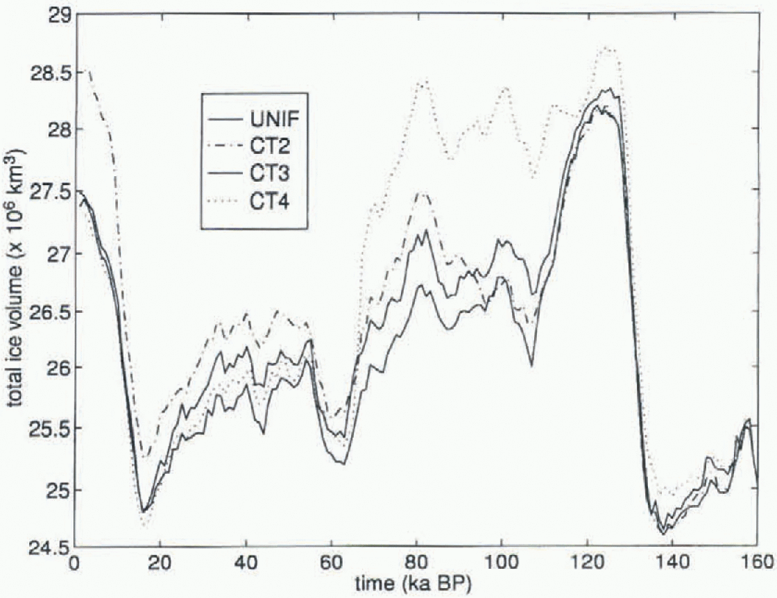
Time-dependent change in total ice volume for CT variable-lithosphere models. Uniform-rigidity model is also shown as the solid line. Major deviations in ice volume occur for CT4 between 120 and 70 ka BP (dotted line) and for CT2 between 55 and 0 ka BP (dot-dashed line).

Jenssen, 1989) with 100 km resolution coupled to an isostatic model with non-uniform lithospheric thickness described above. The time-dependent isostatic adjustment is modelled as a decoupled viscoelastic uniform-manlle-viscosity half-space as described in Cathles (1975). The mantle viscosity is 2 X10²¹Pa S, which is a factor of 2 greater then the customary 1 X 10 ²¹Pas. Reference McConnell and PhinneyMcConnell (1968) notes that a model with decoupled viscoelastic rhcology overestimates the elastic contribution and requires an increase in mantle viscosity to reproduce realistically the observed isostatic adjustment in the Northern Hemisphere.

3. Results

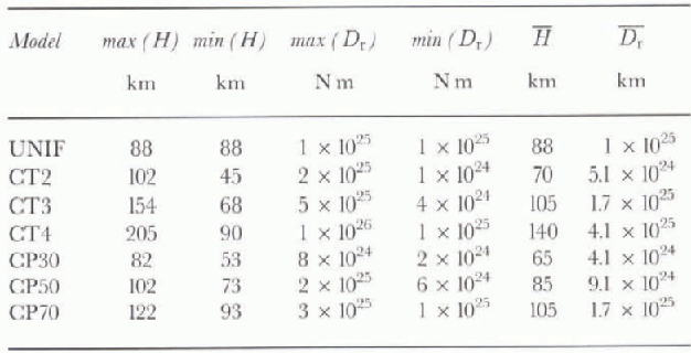
Two relations between crustal thickness and lithospheric thickness are used in the present sensitivity study. The first is linear, and three particular cases are considered where the lithospheric thickness is 2, 3 and 4 times the crustal thickness illustrated in Figure 1. The lithospheric rigidities of these cases span the customary 10²⁵ N m value of uniform rigidity estimates, and are referred to here as CT2, CT3 and CT4. Table 1 shows the main statistical features of each of the models. When the lithospheric thicknesses have been generated they are used in Equation (2) to compute corresponding lithospheric rigidities, and in Equation (4) to generate the matrix A.

The time-dependent changes in total ice-sheet volume generated by the ice-sheet model over a 160 ka Glaciol/inter-Glaciol simulation for CT2, CT3 and CT4 are shown in Figure 2 alongside that of a uniform 10²⁵ N m rigidity model referred to as UNIE It is the time-dependent deviations in ice volume from UNIF that are of interest and two major deviations are noted. CT4 has 1 x10⁶km³ more ice than any of the other models between 120 and 80 ka BP. After 80ka BP the difference disappears and the ice volume generated by CT4 is of similar magnitude to that generated by the other models. The other major difference in ice volume, of 1 X 10⁶ km³, occurs for the CT2 model from 55 ka BP to the present day.

Both of these ice-volume anomalies are positive and

Fig. 3.

Geographical distribution of difference in ice-sheet thickness (in) between CT4 and UNIFat 80 ka BP.

commence during a period of increased accumulation and ice volume over the continent. Figure 3 shows the geographical distribution of differences in ice-sheet thickness at 80 ka between CT4 and UNIE The major differences occur in the interior of West Antarctica and the Ronne and Amery Ice Shelves. Although CT4 is over 100 m thicker in West Antarctica, the major ice-volume anomaly results from differences near the ice shelves of over 500 m. Figure 4 shows the grounding line for CT4 and for UNIFat 80kaBP. It shows that, in the region where the ice-volume differences are greatest, CT4 “grounds” further out onto the continental shelf than UNIE The areas where the ice-volume differences are greatest occur just behind the grounding line.

Fig. 4.

Grounding line at 80 ka for UNIF (thick line) and CT4 (thin line). Major differences in the position of the grounding line occur where the ice-volume differences are maximum.

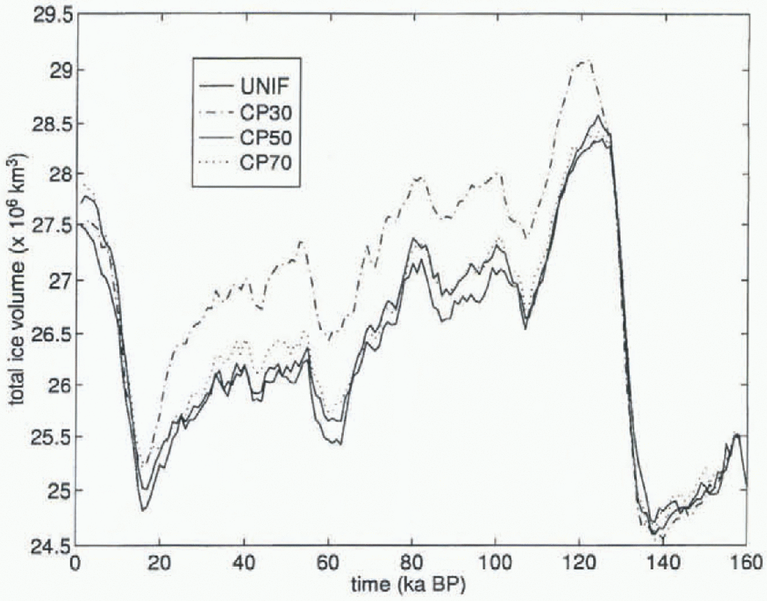
Figure 5 shows the ice-sheet-volume changes as a function of time for three cases of the second type of relation between crustal and lithospheric thickness. The cases are labelled CP30, CP50 and CP70 and correspond to situations where lithospheric thickness is derived by simply adding 30, 50 and 70 km to the crustal thicknesses of Figure I, The maximum, minimum and average field values for these cases are also shown in Table 1. For reference the time-dependent ice-sheet volume generated by UNIF is also shown in Figure 5. The major ice-volume anomaly occurs for CP30, which displays a pattern of behaviour similar to that of CT4 with an ice-volume différence of 1 X 10⁶ km³, but continues throughout the Glaciol period to 20 ka BP. Figure 6 shows the regional ice-volume anomaly, and Figure 7 the grounding-line differences for CP30 and UNIFat 80 ka BP. The ice-volume anomaly for the Amery Ice Shelf is not present for this model run, but there are significant differences near the Ronne Ice Shelf. Figure 7 shows that CP30 has grounded further out onto the continental shelf than UNIF. The pattern of ice-volume anomaly for the CP30 model is similar to that for CT2 and CT4.

4. Discussion

lIn this study the greatest differences in ice volume from UNIF occur for the CT4, CT2 and CP30 models. Table 1 shows the average lithospheric rigidities of the lithosphere for each model. Over a range of averages between 4.1 × 10²⁵ and 4.1 X 10²⁴ N m, large deviations in equilibrium deflection profile and corresponding ice-sheet volume do not occur at large scale in the interior of East Antarctica. The general uniformity of behaviour in the central region beneath East Antarctica for the different lithosphere models can be understood by reference to the first-order equation for uniform lithospheric deformation in Equation (1). The standard two-dimensional Fourier transform is defined as (Reference SneddonSneddon, 1951):

where k_x is the wavenumbcr in the x direction and k_y is the

Fig. 5.

Time-dependent, change in total ice volume for CP variable-lithosphere models. Uniform-rigidity model is also shown as the solid line. Major deviation in ice volume occurs for CP30 between 120 and 20ka BP.

Fig. 6.

Geographical distribution of difference in ice-sheet thickness (m) between CP30 and UNIFat 80 ka BP.

wavenumber in the y direction. Applied to Equation (1), the ratio of ice pressure to induced deflection is:

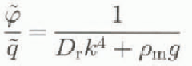
where The presence of D_r in the denominator of Equation (7) shows that the isostatic deflection is inversely dependent on the lithospheric rigidity. However, the importance of the spatial scale of the ice sheet is also apparent because of the presence of the wavenumber k in the denominator. Equation (7) suggests that for an ice sheet of

Fig. 7.

Grounding line at 80 ka for UNIF (thick line) and CP30 (thin line). Major differences in the position of the grounding line occur where the ice-volume differences are maximum.

Table 1.

Maximum, minimum and average values for the effective elastic thickness (H) and lithospheric rigidity (D_T) of the Earth models used in the sensitivity study

wavelength 850 km overlying a lithosphere of rigidity 10²⁵Nm, so that the ice is compensated to an equal degree by both the lithosphere and mantle. As the dominant mode of the wavelength spectrum of the Antarctic ice sheet is a few thousand kilometres, the effect of the lithospheric compensation term is very much less than and the mantle compensation dominates. For the range of values spanned by the lithosphere models in this study, the value of effective lithosphere thickness is unimportant for large wavelengths. in the central region beneath East Antarctica the isostatic deflection is compensated domi-nantly by the mantle so that the lithospheric structure does not play a major role.

The spatial scale of the Antarctic ice sheet is so large that the magnitude of rigidity does not affect the adjustment in the interior of East Antarctica. However, in West Antarctica and at the periphery of the ice sheet near the Ronnc and Amcry Ice Shelves the variable lithospheric model predicts an increased ice-sheet thickness and grounding-line extent compared to the model of uniform rigidity. The spatial scale of the anomalies between the uniform and non-uniform models is small compared to the entire ice sheet, in agreement with the low-pass-filter behaviour of the lithosphere discussed above. The last column in Tabic 1 shows that the models for which this increased ice volume occurs also have the largest deviation in average lithospheric rigidity from the uniform 10²⁵ N m model. The mechanism by which the non-uniform lithospheric-thickness models ground out further onto the continental shelf than the uniform-thick-ness model can be understood as follows: During a period of increased accumulation the advancing ice sheet grounds by capturing the shallow sea floor to its front. The earth responds to this grounding by a regional isostatic deflection caused by the elastic lithosphere. The magnitude of the deflection depends on the regional elasticity of the lithosphere. in particular, a lithosphere model with a large magnitude of regional rigidity produces a smaller deflection then a model with small rigidity. As the deflection at the ice front determines whether further grounding can occur, the regional rigidity controls the extent of ice-sheet grounding.

Figure 8 illustrates this process in a simplified form using a radially symmetric parabolic-profile ice sheet of Antarctic dimensions (3 km thickness and 1000km radius) overlying a lithosphere of variable but radially symmetrical thickness. The lithospheric-rigidily distribution is shown in the top panel, and the resulting equilibrium deflection for each distribution is shown in the central panel. The isostatic

Fig. 8.

Isostatic deflection for a parabolic-profile ice sheet with central height and spatial scale of Antarctic dimensions overlying lithosphere of varying thickness, (a) Rigidity distribution for each lithosphere. (b) Resulting deflection from the application of a parabolic-profile ice sheet with 3 km central thickness and 1000km radius, (c) Fractional deflection anomaly from the uniform-rigidity lithosphere model.

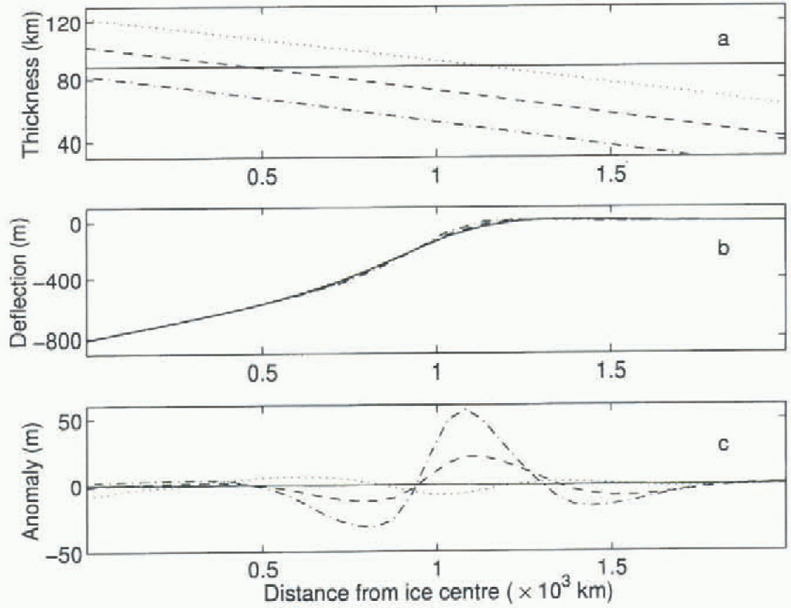
deflection at the centre of the ice sheet is similar for all of the lithospheric structures, verifying that in the interior of the ice sheet the rigidity distribution does not significantly affect the adjustment. However, at the edge of the ice sheet larger deviations in the deflection can be seen. The lower panel shows the deflection anomaly as a fractional difference from the uniform-lilhosphere case. For an ice sheet of this size the anomaly is over 50 m. The anomaly for the lower-rigidity cases is positive at the edge of the ice sheet so that the bedrock elevation is higher there than for the uni-form-lilhospherir-lhickness model. This corresponds to a shallower sea floor then for the uniform-rigidity model, and an increased potential for further grounding by the ice sheet. The anomaly is small, but, as the ice is already grounded near its edge, only slightly reduced deflections cause further grounding.

The analysis presented in Figure 8 ignores several features of the Antarctic ice sheet, such as the time-dependent isostatic adjustment, ice dynamics, hydro-isostasy and lithospheric rigidities that do not have a constant spatial gradient. However, as the lithosphere model is elastic, the deformation pattern of deflection is smoothly varying so that the anomaly from the uniform case is continuous. in this manner, in any region where the anomaly is positive the ice sheet has a greater propensity for further grounding than in the uniform model.

Conclusions

Six different non-uniform lithospheric rigidity profiles have been used to assess the sensitivity of the Antarctic ice sheet to variations in lithospheric rigidity between East and West Antarctica. The major differences in generated ice volume from the uniform-rigidity model occur in West Antarctica and near the Amery and Ronne Ice Shelves, which are both major ire outflow shelves and shallower then the Ross Ice Shelf. The coastal regions near these ice shelves are particularly sensitive to the variation in lithospheric rigidity. The main conclusion of this study is that the importance of nonuniform lithospheric rigidity in models of Glaciol isostasy and ice-sheet behaviour depends on the magnitude and variability of lithospheric thickness. The complex pattern of ice-volume changes is not easily understandable as a simple function of the crustal relations used in this study. The most important question in this study is whether the rigidity distributions assumed in this study are realistiC. Stern and Ten Brink's regional estimate for East and West Antarctica would suggest that the profiles of rigidity used here are reasonable. Kaufmann and Wolf's work to resolve the lateral structure of the earth around the Svalbard archipelago concludes that the ability to resolve the differences in litho-spheric Structure from relative-sea-level data is highly sensitive to the ice-sheet déglaciation history assumed for the region, with lithospheric thicknesses between 0 and 200 km (bund to satisfy the relative sca-lcvcl data. The present work concludes that the ice sheet is sensitive to variations in the lithospheric structure, while Kaufmann and Wolf conclude that the inference of lithospheric structure is sensitive to variations in the ice sheet. Therefore the process of deducing one from the other would not appear straightforward. However, with the results presented here the regions more sensitive to lithospheric variation and corresponding ice behaviour for the Antarctic ice sheet can be outlined. The West Antarctic ice shelves are thought to be primarily responsible for contributing towards an increase of ice volume in Antarctica during the Last Glaciol Maximum (Huybrechts, 1990) and are considered also to be the region of the ice sheet most sensitive to increases in CO₂ levels. The present study suggests that models of Glaciol isostasy using uniform lithospheric thickness underestimate the ice volume generated at coastal margins near the major tee shelves. As the value of lithospheric rigidity used in these models has been derived from studies analyzing relative-sea-level data from predominantly continental regions, the sensitivity of the ice shelves to models of non-uniform lithospheric thickness needs to be further examined.