1 Introduction
Ever since the seminal study by Coles (Reference Coles1956) it has become customary to represent the streamwise mean velocity profile of turbulent boundary layers as a function of the wall-normal coordinate
 $z$
by an addition of a log law and a wake function according to
 $$\begin{eqnarray}U^{+}=\frac{1}{\unicode[STIX]{x1D705}}\ln (z^{+})+A+\frac{2\unicode[STIX]{x1D6F1}}{\unicode[STIX]{x1D705}}W(\unicode[STIX]{x1D702}).\end{eqnarray}$$
Here,
 $\unicode[STIX]{x1D705}$
and
 $A$
are the log-law constants;
 $U^{+}=U/U_{\unicode[STIX]{x1D70F}}$
and
 $z^{+}=zU_{\unicode[STIX]{x1D70F}}/\unicode[STIX]{x1D708}$
, where
 $U_{\unicode[STIX]{x1D70F}}$
is the friction velocity and
 $\unicode[STIX]{x1D708}$
is the kinematic viscosity. The so-called wake function
 $W$
describes the departure from the pure log-law behaviour observed in the outer region of turbulent boundary layers. This region is considered to scale in outer variables
 $\unicode[STIX]{x1D702}=z/\unicode[STIX]{x1D6FF}$
(
 $\unicode[STIX]{x1D6FF}$
being the boundary layer thickness as defined by Chauhan, Monkewitz & Nagib Reference Chauhan, Monkewitz and Nagib2009). Usually, the wake function is normalized such that
 $W(\unicode[STIX]{x1D702}=1)=1$
, and thus the wake parameter
 $\unicode[STIX]{x1D6F1}$
characterizes the strength of the wake in terms of the deviation from the log law at
 $\unicode[STIX]{x1D702}=1$
(e.g. Chauhan et al.
Reference Chauhan, Monkewitz and Nagib2009; Marusic et al.
Reference Marusic, Chauhan, Kulandaivelu and Hutchins2015).
More recently, Chauhan et al. (Reference Chauhan, Monkewitz and Nagib2009) proposed a composite profile fit involving exponential functions for boundary layers and – employing adapted versions – for pipe and channel data (Nagib & Chauhan Reference Nagib and Chauhan2008). The main value of fits of this kind is that they enable calculation of flow properties such as
 $\unicode[STIX]{x1D6FF}$
or
 $\unicode[STIX]{x1D6F1}$
as unambiguously as possible (cf. the discussion in Chauhan & Nagib Reference Chauhan and Nagib2008).
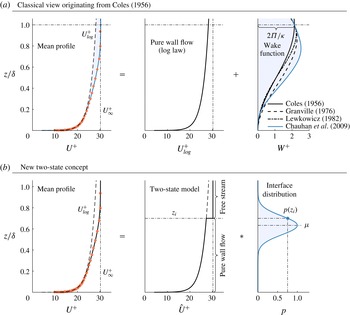
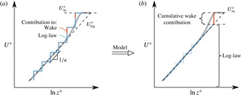
Figure 1(a) illustrates the classical concept of decomposing the velocity profile into a pure wall flow contribution following the log law
 $U_{log}^{+}=1/\unicode[STIX]{x1D705}\ln (z^{+})+A$
and the wake component based on a sample measurement at
 $Re_{\unicode[STIX]{x1D70F}}=10\,500$
(with
 $Re_{\unicode[STIX]{x1D70F}}=U_{\unicode[STIX]{x1D70F}}\unicode[STIX]{x1D6FF}/\unicode[STIX]{x1D708}$
) taken from Marusic et al. (Reference Marusic, Chauhan, Kulandaivelu and Hutchins2015). Here and in the following, we use the term pure wall flow to refer to the self-similar inertial region of the boundary layer. Further, estimates of
 $\unicode[STIX]{x1D6FF}$
and
 $U_{\unicode[STIX]{x1D70F}}$
are obtained from the composite velocity profile fit by Chauhan et al. (Reference Chauhan, Monkewitz and Nagib2009), which makes use of an exponential wake function. Alternative wake formulations proposed by Coles (Reference Coles1956), Granville (Reference Granville1976) and Lewkowicz (Reference Lewkowicz1982) are also included in figure 1(a) for reference.
(a) Illustration of the classical approach of decomposing the mean streamwise velocity profile into additive contributions of pure wall flow and a wake component (shown as blue shaded area) that accounts for deviations from the log law. The blue line represents the wake formulation of Chauhan et al. (Reference Chauhan, Monkewitz and Nagib2009) which was used to fit the experimental data at
 $Re_{\unicode[STIX]{x1D70F}}=10\,500$
(red symbols in both panels). (b) Sketch of the concept proposed here which represents the mean velocity profile via a two-state model comprising pure wall flow and the free stream. These two states are joint by a velocity jump at the interface and the full profile is recovered by convolution (indicated using the symbol *) of the model profile with the probability distribution of the interface position
 $z_{i}$
.

The model constants required to describe the flow in terms of the two-state model proposed here pertain to parameters of the probability distribution
 $p$
of the interface position
 $z_{i}$
separating the two states (pure wall flow and the free stream) as shown in figure 1(b). The mean profile is obtained by the convolution of the two-state profile and the distribution
 $p$
.
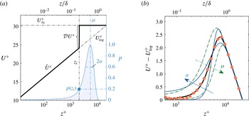
(a) Illustration of the velocity distribution
 $\hat{U} ^{+}$
according to (2.2) (thick solid line) and of the probability density function
 $p$
given by (2.3). (b) Sample best fit (thick black line) to the turbulent boundary layer data at
 $Re_{\unicode[STIX]{x1D70F}}=10\,500$
(red symbols) along with representations of
 $U_{mod}^{+}$
where
 $\unicode[STIX]{x1D70E}$
is varied by
 $\pm 40\,\%$
(thin blue lines) and
 $\unicode[STIX]{x1D707}$
by
 $\pm 20\,\%$
(dashed-dotted green), independently.

Conceptually, the new approach seems appealing since it conforms with the widely observed fact that the boundary layer height fluctuates in time. Moreover, the two-state concept is not restricted to the mean velocity but can be transferred to the streamwise turbulent intensity as will be demonstrated in § 2.2. We do, however, emphasize that the interface in the two-state model is not identical to a turbulent/non-turbulent interface (TNTI). This point will be further elaborated in § 4. Before that, we will introduce the new concept in detail in § 2, confirm its compatibility with the traditional view as well as extend its applicability to pipe and channel flows. The model is then assessed against data in § 3.
2 Wake model
The general idea of decomposing the flow into a pure wall flow and a free stream state is not limited to the streamwise velocity and we will apply the concept to the turbulence intensity later on. However, for the sake of clarity we will introduce the mathematical details as applied to the mean velocity profile first.
For every interface position,
 $z_{i}$
, we define a velocity profile that consists of a log law for
 $z<z_{i}$
and a jump up to
 $U_{\infty }^{+}$
at
 $z_{i}$
given by
 $$\begin{eqnarray}\hat{U} ^{+}\equiv \left\{\begin{array}{@{}ll@{}}{\displaystyle \frac{1}{\unicode[STIX]{x1D705}}}\ln (z^{+})+A,\quad & z<z_{i},\\ U_{\infty }^{+},\quad & z\geqslant z_{i}.\end{array}\right.\end{eqnarray}$$
Using the Heaviside function
 ${\mathcal{H}}$
(2.1) can be expressed by
 $$\begin{eqnarray}\hat{U} ^{+}=U_{log}^{+}{\mathcal{H}}(z_{i}-z)+U_{\infty }^{+}{\mathcal{H}}(z-z_{i}),\end{eqnarray}$$
where
 $U_{log}^{+}\equiv 1/\unicode[STIX]{x1D705}\ln (z^{+})+A$
denotes the log law. We note that
 $z_{i}$
is kept in dimensional units here without loss of generality since any normalization will cancel out eventually as will become evident from (2.5). As outlined above, in addition to (2.2) the shape of the mean profile is also governed by the probability density function (p.d.f.) of the interface position
 $z_{i}$
about which assumptions need to be made. The most straightforward choice is to assume a random independent processes implying a Gaussian distribution given by
 $$\begin{eqnarray}p(z_{i};\unicode[STIX]{x1D707},\unicode[STIX]{x1D70E})\equiv \frac{1}{\unicode[STIX]{x1D70E}\sqrt{2\unicode[STIX]{x03C0}}}\text{e}^{-(z_{i}-\unicode[STIX]{x1D707})^{2}/(2\unicode[STIX]{x1D70E}^{2})},\end{eqnarray}$$
where the two free parameters are the mean
 $\unicode[STIX]{x1D707}$
and the standard deviation
 $\unicode[STIX]{x1D70E}$
. Physically,
 $\unicode[STIX]{x1D707}$
is the mean
 $z$
-location of the interface in the two-state model and
 $\unicode[STIX]{x1D70E}$
describes the extent to which it is fluctuating around
 $\unicode[STIX]{x1D707}$
. An illustration of
 $\hat{U} ^{+}$
along with
 $p$
is provided in figure 2(a). The modelled mean velocity profile
 $U_{mod}^{+}$
is obtained from
 $\hat{U} ^{+}$
and
 $p$
via convolution according to
 $$\begin{eqnarray}U_{mod}^{+}\equiv \int _{0}^{\infty }\hat{U} ^{+}\,p\,\text{d}z_{i}=U_{log}^{+}\left(1-E\right)+U_{\infty }^{+}E,\end{eqnarray}$$
where
 $$\begin{eqnarray}E(z;\unicode[STIX]{x1D707},\unicode[STIX]{x1D70E})=\frac{1}{2}\left[1+\text{erf}\left(\frac{z-\unicode[STIX]{x1D707}}{\sqrt{2\unicode[STIX]{x1D70E}^{2}}}\right)\right].\end{eqnarray}$$
To allow for a closed form solution, the lower limit of the integral in (2.4) was extended to
 $-\infty$
which, in good agreement with the results presented later, assumes that
 $p(z_{i}<0)\ll 1$
.
A sample fit to turbulent boundary layer (TBL) data with
 $U_{log}^{+}$
subtracted is displayed in figure 2(b) illustrating that the shape of
 $U_{mod}^{+}$
allows excellent collapse with the data in the wake region. In the same plot we also show the effect of varying
 $\unicode[STIX]{x1D707}$
and
 $\unicode[STIX]{x1D70E}$
independently of each other.
2.1 Velocity deficit form
The compatibility of the new formulation with the additive concept of Coles (Reference Coles1956) is best demonstrated in the velocity deficit form. For this purpose, (2.4) is restated as
 $$\begin{eqnarray}U_{\infty }^{+}-U_{mod}^{+}=\left(U_{\infty }^{+}-U_{log}^{+}\right)(1-E).\end{eqnarray}$$
Expressing the log law in outer scales leads to the classical velocity deficit form
 $$\begin{eqnarray}U_{\infty }^{+}-U_{mod}^{+}=-\frac{1}{\unicode[STIX]{x1D705}}\ln \unicode[STIX]{x1D702}+\left[E\frac{1}{\unicode[STIX]{x1D705}}\ln \unicode[STIX]{x1D702}+\unicode[STIX]{x1D6F9}\left(1-E\right)\right],\end{eqnarray}$$
with
 $$\begin{eqnarray}\unicode[STIX]{x1D6F9}\equiv U_{\infty }^{+}-\frac{1}{\unicode[STIX]{x1D705}}\ln Re_{\unicode[STIX]{x1D70F}}-A\end{eqnarray}$$
and
 $Re_{\unicode[STIX]{x1D70F}}=U_{\unicode[STIX]{x1D70F}}\unicode[STIX]{x1D6FF}/\unicode[STIX]{x1D708}=\unicode[STIX]{x1D6FF}^{+}$
. The term in the brackets in (2.7) is equivalent to the wake function in outer normalization and by evaluating (1.1) at
 $\unicode[STIX]{x1D6FF}^{+}$
it follows that
 $\unicode[STIX]{x1D6F9}=(2\unicode[STIX]{x1D6F1}/\unicode[STIX]{x1D705})W(\unicode[STIX]{x1D702}=1)$
. Defining the wake parameter
 $\unicode[STIX]{x1D6F1}$
based on the deviation from the log law at
 $\unicode[STIX]{x1D702}=1$
, i.e. normalizing
 $W$
such that
 $W(\unicode[STIX]{x1D702}=1)=1$
, we find for the model
 $$\begin{eqnarray}(U_{mod}^{+}-U_{log}^{+})\big|_{\unicode[STIX]{x1D702}=1}\equiv \frac{2\unicode[STIX]{x1D6F1}}{\unicode[STIX]{x1D705}}=\unicode[STIX]{x1D6F9}E(\unicode[STIX]{x1D702}=1;\unicode[STIX]{x1D707},\unicode[STIX]{x1D70E}).\end{eqnarray}$$
Hence, the new formulation is consistent with the classical law of the wake (i.e.
 $\unicode[STIX]{x1D6F1}=\text{const.}$
) if
 $E(\unicode[STIX]{x1D702}=1)\neq f(Re_{\unicode[STIX]{x1D70F}})$
. This will be established from the data in § 3. Further, it is required that
 $\unicode[STIX]{x1D6F9}=\text{const.}$
, which we confirm in appendix A for the canonical wall-bounded flows based on friction laws for the respective geometries. This consistency would seem to indicate why the classical model appears to work so well, even though the interpretation and physical underpinning are distinctively different.
Note that by (2.9) the condition that
 $U_{mod}^{+}(\unicode[STIX]{x1D702}=1)=U_{\infty }^{+}$
implies that
 $E(\unicode[STIX]{x1D702}=1)$
should be unity. However, we do not enforce this condition explicitly so as not to prioritize a single
 $z$
-location in the fitting and instead let the outcome of the fit determine
 $E(\unicode[STIX]{x1D702}=1)$
. This will be discussed further when we present the data. Furthermore,
 $E(\unicode[STIX]{x1D702}=1;\unicode[STIX]{x1D707},\unicode[STIX]{x1D70E})=\text{const.}$
if the argument of the error function in (2.5) is constant. This is the case if
 $\unicode[STIX]{x1D712}\equiv (1-\unicode[STIX]{x1D707})/\sqrt{2\unicode[STIX]{x1D70E}^{2}}=\text{const.}$
, such that
 $E(\unicode[STIX]{x1D702}=1)$
is
 $f(\unicode[STIX]{x1D712})$
only.
2.2 Streamwise turbulence intensity
Apart from the log law for the mean velocity, Townsend’s attached eddy hypothesis suggests that pure wall flow is also characterized by a log law for the streamwise turbulence intensity
 $\overline{u^{2}}^{+}$
(Townsend Reference Townsend1976). Other theoretical approaches arrive to the same result (Hultmark Reference Hultmark2012). If, as presented above, the outer parts of the velocity profile can be interpreted in terms of the simple two-state model, then an intriguing proposition is that the model should also predict the roll-off of the streamwise turbulence intensity
 $\overline{u^{2}}^{+}$
in the wake region. Analogous to the analysis for the streamwise velocity above, we model the turbulence intensity profile as
 $$\begin{eqnarray}\hat{u} ^{2+}\equiv \left\{\begin{array}{@{}ll@{}}B_{1}-A_{1}\ln (\unicode[STIX]{x1D702}),\quad & z<z_{i},\\ \overline{u^{2}}_{\infty }^{+},\quad & z\geqslant z_{i},\end{array}\right.\end{eqnarray}$$
which again can be restated using the Heaviside function
 ${\mathcal{H}}$
as
 $$\begin{eqnarray}\hat{u} ^{2+}=\overline{u^{2}}_{log}^{+}(\unicode[STIX]{x1D702}){\mathcal{H}}(z_{i}-z)+\overline{u^{2}}_{\infty }^{+}{\mathcal{H}}(z-z_{i}),\end{eqnarray}$$
where,
 $\overline{u^{2}}_{log}^{+}=B_{1}-A_{1}\ln (\unicode[STIX]{x1D702})$
is the log law for
 $\overline{u^{2}}^{+}$
with constants
 $A_{1}$
and
 $B_{1}$
(Marusic et al.
Reference Marusic, Monty, Hultmark and Smits2013). The
 $\overline{u^{2}}_{\infty }^{+}$
-term accounts for the free stream turbulence intensity in cases in which it is not negligible. Analogous to (2.4) convolution with
 $p$
yields
 $$\begin{eqnarray}\overline{u^{2}}_{mod}^{+}=\overline{u}_{log}^{2+}\left[1-E(z;\unicode[STIX]{x1D70E},\unicode[STIX]{x1D707})\right]+\overline{u^{2}}_{\infty }^{+}E(z;\unicode[STIX]{x1D70E},\unicode[STIX]{x1D707}).\end{eqnarray}$$
The expression (2.12) is predictive in the sense that the value
 $\unicode[STIX]{x1D707}$
and
 $\unicode[STIX]{x1D70E}$
are adopted from the results for the mean velocity profile. No additional fitting is required to model the variance profile.
Monkewitz & Nagib (Reference Monkewitz and Nagib2015) recently argued that the slope
 $A_{1}$
for turbulent boundary layers should be a function of
 $Re_{\unicode[STIX]{x1D70F}}$
. However, the dependence is
 $\propto 1/U_{\infty }^{+}$
and therefore rather weak over the range of available experimental data. Consequently, we follow the more conventional approach of using a fixed slope here as it represents the data reasonably well. In any case, the formulation in (2.10) can easily be changed to account for varying
 $A_{1}$
.
2.3 Extension to channel and pipe flow
It is not immediately obvious why the two-state approach should also be applicable to enclosed geometries such as channel and pipe flows as they are commonly regarded as ‘fully turbulent’ in the sense that in the fully developed flow no non-turbulent free stream exists. Nonetheless, in the light of more recent results this picture needs to be revised slightly. As Kwon et al. (Reference Kwon, Philip, de Silva, Hutchins and Monty2014) show based on channel data up to
 $Re_{\unicode[STIX]{x1D70F}}=4000$
, there exists a distinguished uniform momentum zone, the so-called ‘quiescent core’, in turbulent channel flow that bears resemblance with the free stream of TBLs. In particular, this core is observed to have a high velocity magnitude and low turbulence levels. Similar observations are also described for pipe flow in Kwon (Reference Kwon2016) using data at
 $Re_{\unicode[STIX]{x1D70F}}=1000$
. With the caveat that these studies were performed at relatively low
 $Re_{\unicode[STIX]{x1D70F}}$
, there thus appears to be good reason to believe that the two-state model outlined above might also be suitable for channel and pipe flows. We will test this presumption in the following by simply replacing the free stream velocity
 $U_{\infty }$
by the respective centreline velocity
 $U_{cl}$
, and
 $\unicode[STIX]{x1D6FF}$
by the channel half-width and the pipe radius.
3 Results
For the present study we use smooth-wall zero-pressure gradient turbulent boundary layer data from the Melbourne wind tunnel previously reported in Marusic et al. (Reference Marusic, Chauhan, Kulandaivelu and Hutchins2015) for
 $2800<Re_{\unicode[STIX]{x1D70F}}<13\,400$
and Squire et al. (Reference Squire, Morrill-Winter, Hutchins, Schultz, Klewicki and Marusic2016) for
 $Re_{\unicode[STIX]{x1D70F}}=21\,700$
and 26 800. Further, we employ the superpipe measurements of Hultmark et al. (Reference Hultmark, Vallikivi, Bailey and Smits2012) to evaluate our model for pipe flow, and channel flows are studied using data from direct numerical simulations of Lee & Moser (Reference Lee and Moser2015) and experiments by Schultz & Flack (Reference Schultz and Flack2013).
3.1 Mean velocity
The wake model presented here presumes the existence of a log law with known constants. For the following analysis we adopt the values of
 $\unicode[STIX]{x1D705}$
and
 $A$
from Chauhan et al. (Reference Chauhan, Monkewitz and Nagib2009) for the TBL (
 $\unicode[STIX]{x1D705}=0.384$
,
 $A=4.17$
), the ones given by Marusic et al. (Reference Marusic, Monty, Hultmark and Smits2013) for pipe flow (
 $\unicode[STIX]{x1D705}=0.391$
,
 $A=4.34$
) and the constants provided by Lee & Moser (Reference Lee and Moser2015) for channel flow (
 $\unicode[STIX]{x1D705}=0.384$
,
 $A=4.27$
). However, it is noted that the results are virtually indistinguishable in our figures when alternative pairs of log-law constants suggested in the literature are used. We further obtain estimates of
 $\unicode[STIX]{x1D6FF}$
and
 $U_{\unicode[STIX]{x1D70F}}$
in the TBL from the composite velocity fit by Chauhan et al. (Reference Chauhan, Monkewitz and Nagib2009). While
 $\unicode[STIX]{x1D6FF}$
is not a parameter in the model and is only used to put our results in relation, the
 $U_{\unicode[STIX]{x1D70F}}$
-value from the fit is employed in lieu of a direct measurement of the wall shear stress. Given the distribution parameters
 $\unicode[STIX]{x1D707}$
and
 $\unicode[STIX]{x1D70E}$
both quantities could equivalently be determined from the present fit. Our model does not account for the viscous region close the wall and we consequently only consider the region
 $z^{+}\gtrsim 3Re_{\unicode[STIX]{x1D70F}}^{1/2}$
based on an estimate for the start of the log region (e.g. Marusic et al.
Reference Marusic, Monty, Hultmark and Smits2013). Results of a nonlinear least squares fit of (2.4) with
 $\unicode[STIX]{x1D707}$
and
 $\unicode[STIX]{x1D70E}$
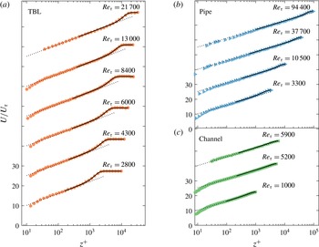
as free parameters to experimental TBL data are presented in figure 3(a). Note that here and in the following, for the sake of clarity results are only shown for approximately half of the available data points. This comes at no loss as the displayed results cover the full range of
 $Re_{\unicode[STIX]{x1D70F}}$
available and are representative of the full dataset. Excellent agreement of the fitted model with the data is observed from the start of the log law all throughout the wake region over the full range of
 $Re_{\unicode[STIX]{x1D70F}}$
displayed. Similar observations can be made for pipe (figure 3
b) and channel flow (figure 3
c), even with a weaker wake in those flows.
Fit according to (2.4) (shown as black lines) to mean profiles of mean streamwise velocity (symbols) in (a) TBL, (b) pipe flow and (c) channel flow. All fits are shown for
 $z^{+}>3Re_{\unicode[STIX]{x1D70F}}^{1/2}$
. The vertical shift between individual profiles is 15.

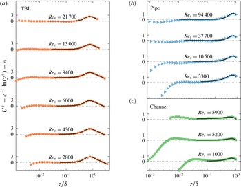
To highlight the wake region, we present the same profiles as in figure 3 once more in figure 4 but this time with
 $U_{log}^{+}$
subtracted in order to scrutinize the deviations from the log law in the wake region. Again, the wake profile for boundary layers (figure 4
a) is very well approximated by the fit. As is evident from figures 4(b) and 4(c), also the departure from the log law in the outer regions of pipe and channel flows can be captured very accurately using the two-state model.
Same as figure 3 but with the log law subtracted to focus on the wake region.

Having established that the wake formulation of (2.4) can be fitted to closely match the data for all three flow cases considered, it is instructive to study the fit parameters
 $\unicode[STIX]{x1D707}$
and
 $\unicode[STIX]{x1D70E}$
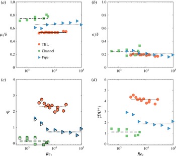
, which are plotted in figure 5(a,b) as a function of
 $Re_{\unicode[STIX]{x1D70F}}$
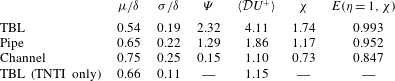
(their mean values are reported in table 1). Consistent with the expectation based on the law of the wake, we find that the mean and the standard deviation of the fitted interface p.d.f. are constant to very good approximation over the full range of
 $Re_{\unicode[STIX]{x1D70F}}$
in all flows. Differences between the different geometries are most pronounced for
 $\unicode[STIX]{x1D707}$
in figure 5(a). Lower values of
 $\unicode[STIX]{x1D707}$
lead to stronger mean velocity jumps (discussed in more detail below) and hence a more pronounced wake function. The trend of increasing
 $\unicode[STIX]{x1D707}$
in the order TBL, pipe, channel is therefore in agreement with the trend for the wake strength of those flows (Monty et al.
Reference Monty, Hutchins, Ng, Marusic and Chong2009).
Fit parameters (a)
 $\unicode[STIX]{x1D707}$
and (b)
 $\unicode[STIX]{x1D70E}$
. (c)
 $\unicode[STIX]{x1D6F9}$
values from (2.9) using the fit result for
 $E(\unicode[STIX]{x1D702}=1)$
(filled symbols) from and from the definition (2.8) (open symbols). Horizontal black lines indicate the mean of
 $\unicode[STIX]{x1D6F9}$
from (2.8) over all
 $Re_{\unicode[STIX]{x1D70F}}$
for the respective flow; coloured horizontal lines represent the respective
 $\unicode[STIX]{x1D6F9}$
values from friction laws as derived in appendix A. (d) Mean velocity jump
 $\langle {\mathcal{D}}U^{+}\rangle$
(symbols) along with the mean (horizontal lines). In all panels results are shown for TBL (red circles, solid line), pipe flow (blue triangles, dotted line) and channel flow (green squares, dashed line). Horizontal lines represent the respective mean values, which are also listed in table 1. Note that in (c) and (d) the lowest two
 $Re_{\unicode[STIX]{x1D70F}}$
values for pipe flow were excluded from the mean.

The variations of
 $\unicode[STIX]{x1D70E}$
between the geometries are relatively small,
 $\unicode[STIX]{x1D70E}/\unicode[STIX]{x1D6FF}\approx 0.2$
with a slight increasing tendency with increasing wake strength. The mean value of
 $\unicode[STIX]{x1D712}$
listed in table 1 should be large enough such that
 $E(\unicode[STIX]{x1D702}=1,\unicode[STIX]{x1D712})\rightarrow 1$
. For the TBL this condition is met with very high accuracy which is indicative of how well the modelled profile fits the data. For the internal geometries,
 $\unicode[STIX]{x1D712}$
is somewhat smaller and hence
 $E(\unicode[STIX]{x1D702}=1)$
is slightly lower than expected (cf. table 1). Using the values of
 $\unicode[STIX]{x1D6F9}$
plotted in figure 5(c), the differences between
 $E(\unicode[STIX]{x1D702}=1)$
and unity correspond to a deviation from
 $U_{\infty }^{+}$
at
 $\unicode[STIX]{x1D702}=1$
of
 $0.016U_{\unicode[STIX]{x1D70F}}$
(TBL),
 $0.062U_{\unicode[STIX]{x1D70F}}$
(pipe) and
 $0.023U_{\unicode[STIX]{x1D70F}}$
(channel). These small differences characterize (as an upper bound since
 $\unicode[STIX]{x1D702}=1$
is at the edge of the fitted region) how well the shape of the model represents the actual wake profile. One possible explanation for the slightly inferior fit (relative to the wake strength) for the internal geometries is the fact that the model does not account for interactions across the centreline. At least in channel flow, such events are possible, albeit rare (Kwon et al.
Reference Kwon, Philip, de Silva, Hutchins and Monty2014).
Additionally, we show estimates for
 $\unicode[STIX]{x1D6F9}$
derived from friction laws in figure 5(c) (see appendix A for details) which match the means computed from (2.8) closely.
The ‘velocity jump’ for a given interface position
 $z_{i}$
is given by (cf. figure 2)
 $$\begin{eqnarray}{\mathcal{D}}U^{+}=U_{\infty }^{+}-U_{log}^{+}(z_{i})\end{eqnarray}$$
and based on the fit results for
 $p(z_{i})$
a mean jump can be obtained from
 $$\begin{eqnarray}\langle {\mathcal{D}}U^{+}\rangle =\int _{0}^{\unicode[STIX]{x1D6FF}}{\mathcal{D}}U^{+}p(z_{i})\,\text{d}z_{i}.\end{eqnarray}$$
Results for
 $\langle {\mathcal{D}}U^{+}\rangle$
are shown in figure 5(d) and the mean over all
 $Re_{\unicode[STIX]{x1D70F}}$
is tabulated in table 1. The trends again fall in line with observations for the wake parameters with
 $\langle {\mathcal{D}}U^{+}\rangle$
in TBL being considerably higher than for the internal flows. Apart from pipe flow below
 $Re_{\unicode[STIX]{x1D70F}}=3400$
, there does not appear to be a dependence of
 $\langle {\mathcal{D}}U^{+}\rangle$
on
 $Re_{\unicode[STIX]{x1D70F}}$
.
Overview over all parameters of the wake model. The line labelled ‘TNTI only’ additionally presents properties of the turbulent/non-turbulent interface as reported in Chauhan, Philip & Marusic (Reference Chauhan, Philip and Marusic2014a ) for reference.

3.2 Streamwise turbulence intensity
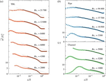
A comparison of (2.12) to the actual data is shown in figure 6. The required log-law constants for the different flows are adopted from Marusic et al. (Reference Marusic, Monty, Hultmark and Smits2013) and listed in the caption of the figure. There are obvious limitations, especially for the internal geometries at lower
 $Re_{\unicode[STIX]{x1D70F}}$
where the data do not comply very well with the log law used. However, at higher Reynolds numbers there is good agreement between the predicted and the actual shape of the roll-off in the wake region for all geometries, suggesting that the behaviour of
 $\overline{u^{2}}^{+}$
in the outer region can indeed be captured with the proposed model. It is stressed here once again that no additional fitting is involved in modelling the variance profiles as the fit parameters
 $\unicode[STIX]{x1D707}$
and
 $\unicode[STIX]{x1D70E}$
are adopted from the mean velocity fit.
Even though the overall agreement of the model with the data is very good, a slight but consistent difference is observed between the model prediction and the data for
 $0.5<z/\unicode[STIX]{x1D6FF}<0.8$
in the TBL. As Kwon, Hutchins & Monty (Reference Kwon, Hutchins and Monty2016) (see also Kwon Reference Kwon2016) have shown, TNTI oscillations ‘contaminate’ the fluctuating field in the outer region of wall-bounded flows. By comparing to an alternative decomposition based on averages conditioned on the TNTI position, they demonstrated that the classical Reynolds decomposition leads to slightly higher fluctuation levels where the flow is intermittent. This intermittency effect is not captured in the present two-state model which might explain the minor discrepancy. At least in location and magnitude the difference observed here is similar to the variations between results based on the Reynolds decomposition and on a decomposition using conditional means in Kwon (Reference Kwon2016). A similar trend would be expected for internal flows as well. However, it is even harder to detect there due to the smaller wake strength in internal flows.
Profiles of
 $\overline{u^{2}}^{+}$
(symbols) along with predictions according to (2.12) (solid black lines) using
 $B_{1}=2.2$
for TBL in (a),
 $B_{1}=1.56$
for the pipe data in (b) and
 $B_{1}=2$
in channel flow (c), while
 $A_{1}=1.26$
is kept the same in all cases. The free stream value
 $\overline{u^{2}}_{\infty }^{+}$
is set to 0 (TBL), 0.8 (pipe), and 0.6 (channel). The offset between profiles is
 $10$
.

4 Discussion
An obvious question is how the two-state model relates to the TNTI and intermittency, which have been studied extensively in TBLs. Recently, Chauhan et al. (Reference Chauhan, Philip and Marusic2014a
) have demonstrated that a link between the TNTI and the wake profile exists by showing that an idealized velocity jump correlated with the p.d.f. of the TNTI position yields good agreement with the outer part of the wake region where
 $\unicode[STIX]{x1D702}>0.6$
. However, they also realized that the actual measured velocity jump was insufficient to explain the full wake strength (in fact, they use a jump value that is 1.7 times the one measured across the TNTI).
Similarly, the mean velocity jump from the present two-state model for the TBL is
 $4.1U_{\unicode[STIX]{x1D70F}}$
, which is almost four times the TNTI-value of
 $1.15U_{\unicode[STIX]{x1D70F}}$
reported in Chauhan et al. (Reference Chauhan, Philip and Marusic2014a
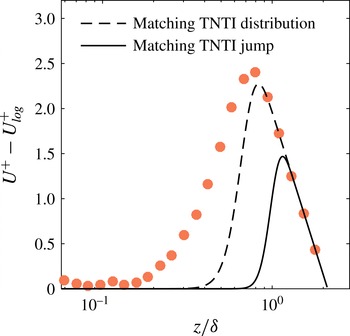
). Further, figure 7 shows results for the model when matching either the distribution of the TNTI position (dashed line, parameters listed in table 1) or the magnitude of the mean jump across the TNTI by adjusting
 $p$
(solid line). Here we chose
 $\unicode[STIX]{x1D707}=\unicode[STIX]{x1D6FF}$
while keeping
 $\unicode[STIX]{x1D70E}/\unicode[STIX]{x1D6FF}=0.11$
. Other combinations are possible but lead to qualitatively similar results. It is clear that in both cases the extent and magnitude of the wake profile are clearly under predicted – even though matching the interface distribution amounts to
 $\langle {\mathcal{D}}U^{+}\rangle \approx 3$
, almost three times the interface jump. This is no surprise in view of the fact that intermittency becomes very small for
 $z/\unicode[STIX]{x1D6FF}<0.4$
(e.g. Chauhan et al.
Reference Chauhan, Philip, de Silva, Hutchins and Marusic2014b
) whereas the wake profile has significant contributions much closer to the wall (cf. figure 1
a).
Results from the two-state model when using TNTI-properties as listed in table 1. Matching the TNTI distribution parameters (dashed line) leads to a value of
 $\langle {\mathcal{D}}U^{+}\rangle \approx 3$
, while the TNTI jump can be matched when
 $\unicode[STIX]{x1D707}=\unicode[STIX]{x1D6FF}$
(solid line). Symbols: experimental TBL data at
 $Re_{\unicode[STIX]{x1D70F}}=10\,500$
.

From the above, it is evident that the interface in the model is not equivalent to the TNTI. A way in which the two-state model could be reconciled with physical observations is sketched in figure 8 and outlined in the following. Adrian, Meinhart & Tomkins (Reference Adrian, Meinhart and Tomkins2000) and more recent studies by Eisma et al. (Reference Eisma, Westerweel, Ooms and Elsinga2015) and de Silva, Hutchins & Marusic (Reference de Silva, Hutchins and Marusic2016) have highlighted the importance of uniform momentum zones (UMZs) and of the shear layers separating them in turbulent wall-bounded flow (but also isotropic turbulence, see e.g. Ishihara, Kaneda & Hunt Reference Ishihara, Kaneda and Hunt2013). Based on these observations, figure 8(a) presents a simplified and idealized instantaneous velocity distribution that consists entirely of UMZs and velocity changes are restricted to jumps across the shear layers separating them. At least on average – but not necessarily instantaneously as depicted in the figure for simplicity – the ‘aspect ratio’ of such UMZs, i.e. the ratio of their wall-normal extent to the magnitude of the adjacent velocity jump, needs to follow a log slope in the region where pure wall flow is observed. The wake profile is then a consequence of ‘excess’ velocity jumps which alter this aspect ratio as shown in the figure. In this context the present model can be interpreted as lumping all the excess jumps (of unknown magnitude and distribution) into a single interface jump as shown in figure 8(b).
It should be emphasized at this point that the ‘excess’ part of the velocity jump is defined relative to the width of the UMZ. For the purpose of a more intuitive illustration we chose to keep the log-scaled wall-normal extent of all uniform momentum zones in figure 8(a) equal. This choice results in larger velocity jumps in the wake region, which is unrealistic. However, the important quantity is only the aspect ratio such that the model is entirely consistent with experimental results showing decreasing velocity jumps with increasing distance off the wall (de Silva et al. Reference de Silva, Hutchins and Marusic2016) if the height of the UMZs decreases accordingly.
Based on the difference between
 $\langle {\mathcal{D}}U^{+}\rangle$
and the TNTI jump in TBLs it may be concluded that the internal shear layers contribute a significant part to the wake profile in this case.
Visualization of a possible interpretation of the two-state concept. (a) Idealized instantaneous velocity distribution illustrating how shear layer jumps contribute to the log-law (blue) and the wake profile (red). For simplicity, the log-scaled wall-normal extent of all uniform momentum zones is assumed to be equal. (b) In the model, all wake contributions are lumped into a single velocity jump. The mean profile is shown as grey line in both panels.

In contrast, the jump at the boundary of the ‘quiescent’ core region of channel flow reported in Kwon et al. (Reference Kwon, Philip, de Silva, Hutchins and Monty2014) is comparable in magnitude to the mean jump from the present model. Hence, this jump is expected to contribute most of the wake deficit which is in line with the fact that a simple zonal average for the wall region in Kwon et al. (Reference Kwon, Philip, de Silva, Hutchins and Monty2014) extends the log law into the wake region with reasonable approximation.
5 Conclusions
We have shown that a simple two-state model, with pure wall flow characterized by a log law as one state and the free stream flow as the other, can be fit to the data with good accuracy. The fitted parameters are the properties of the p.d.f. of the interface location between the two states, which is assumed to be normally distributed. In contrast to the classical concept of representing the wake region by addition of the log law and a wake function, the new model is based on a convolution of the two-state model profile with the p.d.f. of the interface distribution. The interface distribution obtained for TBL from the model is different from the p.d.f. of the TNTI position which confirms that intermittency only accounts for a part of the wake profile in this flow. We offer an interpretation for the full deviation from the log law in the wake region of TBLs as the combined effect of velocity jumps bounding uniform momentum zones and the jump across the TNTI. The model can be thought of as lumping all individual velocity jumps into a single discontinuity and adjusting the interface distribution such that the overall effect is equivalent. In this respect, our model strikes a sensible compromise in representing the underlying physics while limiting the number of free parameters by representing all internal jump and TNTI contributions to the wake with a single velocity jump. Hence, instead of providing merely a new parametrization, the new model leads to a new interpretation of the wake profile that is closer to the actual physics.
We further find that based on the fit of the mean profile, the roll-off in the outer region of the streamwise velocity fluctuations can be predicted with good accuracy. Moreover, the applicability of the model is demonstrated for the canonical wall-bounded flows considered here, namely the zero-pressure gradient boundary layer, pipe, and channel flows, and the results are seen to be consistent with known trends for the wake strength between these flows. Finally, we note that our results for internal geometries, where no TNTI is present, are in line with recent findings on internal shear layers in these geometries reported by Kwon et al. (Reference Kwon, Philip, de Silva, Hutchins and Monty2014, Reference Kwon, Hutchins and Monty2016)
Appendix A.
 $\unicode[STIX]{x1D6F9}$
from friction laws

A.1 Turbulent boundary layers
Using the Rotta–Clauser skin friction relation
 $U_{\infty }^{+}=1/\unicode[STIX]{x1D705}\ln Re_{\unicode[STIX]{x1D6FF}^{\ast }}+C_{bl}$
with
 $C_{bl}=3.3$
(Monkewitz, Chauhan & Nagib Reference Monkewitz, Chauhan and Nagib2007) and substituting into (2.8) we get
 $\unicode[STIX]{x1D6F9}_{bl}=1/\unicode[STIX]{x1D705}\ln Re_{\unicode[STIX]{x1D6FF}^{\ast }}/Re_{\unicode[STIX]{x1D70F}}+C_{bl}-A$
. The ratio of the Reynolds numbers
 $Re_{\unicode[STIX]{x1D6FF}^{\ast }}/Re_{\unicode[STIX]{x1D70F}}=\unicode[STIX]{x1D6E5}/\unicode[STIX]{x1D6FF}$
, where
 $\unicode[STIX]{x1D6E5}$
is the Rotta–Clauser length scale defined by
 $\unicode[STIX]{x1D6E5}=U_{\infty }^{+}\unicode[STIX]{x1D6FF}^{\ast }$
. It has been shown by Chauhan & Nagib (Reference Chauhan and Nagib2008) that
 $\unicode[STIX]{x1D6E5}/\unicode[STIX]{x1D6FF}\rightarrow \text{const.}\approx 3.4$
and hence
 $$\begin{eqnarray}\unicode[STIX]{x1D6F9}_{bl}=\frac{1}{\unicode[STIX]{x1D705}}\ln \frac{\unicode[STIX]{x1D6E5}}{\unicode[STIX]{x1D6FF}}+C_{bl}-A\approx 2.32.\end{eqnarray}$$
A.2 Pipe flow
In pipes the Reynolds number dependence of the friction factor
 $\unicode[STIX]{x1D706}\equiv 8\left(U_{\unicode[STIX]{x1D70F}}/U_{B}\right)^{2}$
is described by the Prandtl equation
 $$\begin{eqnarray}\sqrt{\frac{8}{\unicode[STIX]{x1D706}}}=U_{B}^{+}=\frac{1}{\unicode[STIX]{x1D705}}\ln (Re_{D}\sqrt{\unicode[STIX]{x1D706}})+C_{p},\qquad C_{p}=-1.305\sqrt{8}\end{eqnarray}$$
(equation 11, Furuichi et al.
Reference Furuichi, Terao, Wada and Tsuji2015) where
 $U_{B}$
is the mean streamwise velocity over the pipe cross-section and
 $Re_{D}$
a Reynolds number based on the pipe diameter and
 $U_{B}$
. Substituting
 $Re_{D}\sqrt{\unicode[STIX]{x1D706}}=4\sqrt{2}Re_{\unicode[STIX]{x1D70F}}$
and noting that
 $\unicode[STIX]{x1D709}_{p}\equiv U_{cl}^{+}-U_{B}^{+}\rightarrow \text{const.}\approx 4.267$
(Furuichi et al.
Reference Furuichi, Terao, Wada and Tsuji2015) we get
 $U_{cl}^{+}=1/\unicode[STIX]{x1D705}\ln (Re_{\unicode[STIX]{x1D70F}})+C+1/\unicode[STIX]{x1D705}\ln (4\sqrt{2})+\unicode[STIX]{x1D709}_{p}$
. When inserting this result into (2.8) the
 $Re_{\unicode[STIX]{x1D70F}}$
-terms vanish resulting in
 $$\begin{eqnarray}\unicode[STIX]{x1D6F9}_{pipe}=C_{p}+\frac{1}{\unicode[STIX]{x1D705}}\ln (4\sqrt{2})+\unicode[STIX]{x1D709}_{p}-A\approx 1.29.\end{eqnarray}$$
A.3 Channel flow
In channel flow the friction factor
 $C_{f}\equiv 2(U_{\unicode[STIX]{x1D70F}}/U_{B})^{2}$
and the Prandtl equation is given by
 $$\begin{eqnarray}\sqrt{\frac{2}{C_{f}}}=U_{B}^{+}=\frac{1}{\unicode[STIX]{x1D705}}\ln (Re_{m}\sqrt{C_{f}})+C_{c},\end{eqnarray}$$
where
 $Re_{m}$
is based on the channel height and the average velocity across the channel height
 $U_{B}$
. With these definitions
 $Re_{m}\sqrt{C_{f}}=2\sqrt{2}Re_{\unicode[STIX]{x1D70F}}$
and it is further found that
 $U_{cl}^{+}-U_{B}^{+}\equiv \unicode[STIX]{x1D709}_{c}\rightarrow \text{const.}\approx 2.64$
(Dean Reference Dean1978) such that
 $U_{cl}^{+}=1/\unicode[STIX]{x1D705}\ln (Re_{\unicode[STIX]{x1D70F}})+C_{c}+1/\unicode[STIX]{x1D705}\ln (2\sqrt{2})+\unicode[STIX]{x1D709}_{c}$
, which by inserting into (2.8) leads to
 $$\begin{eqnarray}\unicode[STIX]{x1D6F9}_{channel}=C_{c}+\frac{1}{\unicode[STIX]{x1D705}}\ln (\sqrt{2})+\unicode[STIX]{x1D709}_{c}-A=0.15,\end{eqnarray}$$
where
 $C_{c}=-0.98$
was used (Schultz & Flack Reference Schultz and Flack2013, with the original value of
 $C_{c}=0.03$
adjusted for the slightly different value of
 $\unicode[STIX]{x1D705}$
used here).