1. Introduction
A low-conductivity drop will deform when placed in a weakly conducting medium under a uniform direct current (DC) electric field
 $\boldsymbol{E}_{\infty }$
. The deformation is typically characterized by the scalar parameter
 $D=(r_{1}^{\ast }-r_{2}^{\ast })/(r_{1}^{\ast }+r_{2}^{\ast })$
, where
 $r_{1}^{\ast }$
and
 $r_{2}^{\ast }$
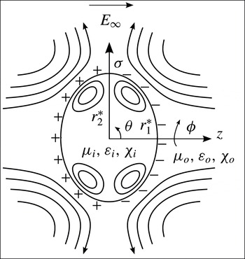
denote the semiaxes along and perpendicular to the applied field respectively (figure 1). Here, the superscript
 $\ast$
is implemented to represent a dimensional quantity or variable; material properties contain no superscript, as they will not subsequently be made dimensionless. In the work of Allan & Mason (Reference Allan and Mason1962), deformations along the applied field (prolate,
 $D>0$
) and normal to the applied field (oblate,
 $D<0$
) were observed experimentally. However, at the time, the existing electrohydrostatic theory developed for two perfect dielectric fluids (O’Konski & Thacher Reference O’Konski and Thacher1953; Allan & Mason Reference Allan and Mason1962) was only able to predict prolate conformations. This discrepancy was resolved by Taylor’s leaky dielectric model (Taylor Reference Taylor1966; Melcher & Taylor Reference Melcher and Taylor1969; Saville Reference Saville1997), which accounts for the finite conductivity of both phases, thereby providing the opportunity for surface charge to arrive at the interface between the suspended drop and the surrounding medium. The action of the electric field on this interfacial charge gives rise to shear electrical stresses, which are absent for perfect dielectrics and conductors. These stresses are balanced by shear viscous stresses; thus, steady fluid motion – an electrohydrodynamic flow – is induced inside and outside of the drop. Taylor’s analysis provided the following expression for the steady-state deformation of a slightly deformed drop:
 $$\begin{eqnarray}D_{T}=\frac{9}{16(2R+1)^{2}}\left[\frac{3R(3M+2)(1-SR)}{5(M+1)}+R^{2}(1-2S)+1\right]\mathit{Ca}_{o}.\end{eqnarray}$$
Schematic of the electric-field-induced oblate deformation of a weakly conducting drop. The drop of viscosity
 ${\it\mu}_{i}$
, permittivity
 ${\it\varepsilon}_{i}$
and resistivity
 ${\it\chi}_{i}$
is suspended in a medium with properties
 ${\it\mu}_{o}$
,
 ${\it\varepsilon}_{o}$
and
 ${\it\chi}_{o}$
respectively. The case considered is that for which the inner charging time scale
 ${\it\tau}_{e,i}={\it\varepsilon}_{i}{\it\chi}_{i}$
is greater than the outer charging time scale
 ${\it\tau}_{e,o}={\it\varepsilon}_{o}{\it\chi}_{o}$
, which yields the surface charge distribution and oblate deformation qualitatively drawn here. The electric field is directed from left to right, while streamlines are depicted inside and outside of the drop. The direction of flow is from the poles (
 ${\it\theta}=0,{\rm\pi}$
) towards the equator (
 ${\it\theta}={\rm\pi}/2$
) of the drop. The electric field and induced fluid flow are both independent of the azimuth
 ${\it\phi}$
. Here, (
 ${\it\sigma},{\it\phi},z$
) corresponds to the set of cylindrical coordinates, while
 ${\it\theta}$
represents the polar angle measured from the positive
 $z$
-axis. The major and minor semiaxes are denoted by
 $r_{2}^{\ast }$
and
 $r_{1}^{\ast }$
respectively.

Here, the deformation
 $D_{T}$
is a function of the permittivity ratio
 $S={\it\varepsilon}_{i}/{\it\varepsilon}_{o}$
, resistivity ratio
 $R={\it\chi}_{i}/{\it\chi}_{o}$
and viscosity ratio
 $M={\it\mu}_{i}/{\it\mu}_{o}$
, where
 ${\it\varepsilon}$
,
 ${\it\chi}$
and
 ${\it\mu}$
represent the permittivity, resistivity and viscosity respectively, while the subscripts
 $i$
and
 $o$
correspond to the inner (drop, subscript
 $i$
) and outer (medium, subscript
 $o$
) phases. This expression is valid to first order in the electric capillary number
 $\mathit{Ca}_{o}={\it\varepsilon}_{o}\,E_{\infty }^{2}\,a/{\it\gamma}$
, which is defined as a ratio of electrical stress
 ${\it\varepsilon}_{o}E_{\infty }^{2}$
to capillary stress
 ${\it\gamma}/a$
, where
 ${\it\gamma}$
denotes the interfacial tension and
 $a$
is the radius of an undeformed drop. To that order, the slightly perturbed drop shape is spheroidal; it may be expressed as
 ${\it\zeta}^{\ast }=a[1+(4/3)D_{T}P_{2}(\cos {\it\vartheta})]$
, where
 $P_{2}$
is the second Legendre polynomial and
 ${\it\vartheta}$
represents the polar angle measured from the direction of the applied field in spherical coordinates. Taylor’s leaky dielectric model qualitatively captures both the prolate and oblate configurations observed in the experiments of Allan & Mason (Reference Allan and Mason1962). Furthermore, Taylor’s article contains an appendix in which the predicted flow directed from the poles towards the equator of the drop is visualized by tracer particles for a silicone oil drop suspended in a mixture of castor oil and corn oil.
Taylor’s model (Taylor Reference Taylor1966) predicts accurate values for the steady deformation at small capillary numbers
 $\mathit{Ca}_{i,o}$
(Vizika & Saville Reference Vizika and Saville1992; Ha & Yang Reference Ha and Yang2000b
; Salipante & Vlahovska Reference Salipante and Vlahovska2010). Here, the double subscript
 $i,o$
is implemented to label a certain quantity for both the drop and the medium, e.g.
 $\mathit{Ca}_{i,o}$
signifies
 $\mathit{Ca}_{i}$
and
 $\mathit{Ca}_{o}$
. The large-capillary-number regime has received computational treatment to enable the prediction of larger nonlinear steady-state deformations of isolated leaky dielectric drops (Sherwood Reference Sherwood1988; Feng & Scott Reference Feng and Scott1996; Feng Reference Feng1999; Lac & Homsy Reference Lac and Homsy2007; Supeene, Koch & Bhattacharjee Reference Supeene, Koch and Bhattacharjee2008; Fernández Reference Fernández2013; Wang et al.
Reference Wang, Dong, Zhang, Wang and Wen2014) as well as their breakup (Sherwood Reference Sherwood1988; Feng & Scott Reference Feng and Scott1996; Feng Reference Feng1999; Lac & Homsy Reference Lac and Homsy2007; Supeene et al.
Reference Supeene, Koch and Bhattacharjee2008). In this nonlinear regime, the stable drop shape need not be spheroidal. Sherwood (Reference Sherwood1988) was the first to numerically calculate the prolate deformation of a weakly conducting drop subjected to a uniform DC electric field. By implementing the boundary integral method to calculate the electrostatic field and flow field, his work predicted the equilibrium drop shapes and unstable configurations for creeping flow, i.e. Reynolds numbers
 $\mathit{Re}_{Flow(i,o)}={\it\rho}_{i,o}Ua/{\it\mu}_{i,o}\rightarrow 0$
, where
 ${\it\rho}_{i,o}$
denotes the density of either phase and
 $U$
is a characteristic flow strength. Additionally, the viscosity ratio was set to unity (
 $M=1$
). Lac & Homsy (Reference Lac and Homsy2007) considered prolate and oblate conformations, and a differing viscosity between the two phases (
 $M\neq 1$
). By performing a thorough investigation of the dimensionless parameter space spanned by
 $S$
,
 $R$
and
 $M$
, they predicted various stable drop configurations, as well as highly nonlinear (e.g. multilobed) shapes and breakup modes. Their work also analysed how a differing viscosity between the drop and the medium can either enhance stability or promote breakup. Both of these works considered either steady-state deformations or breakup of drops under high field strengths.
Lac & Homsy (Reference Lac and Homsy2007) also compared simulation results against two sets of experiments from Ha & Yang (Reference Ha and Yang2000a
), which measured the steady deformation of a castor oil drop immersed in silicone oil at varying electric capillary number
 $\mathit{Ca}_{o}$
. To calculate the interfacial tension
 ${\it\gamma}$
, Lac and Homsy rescaled the capillary number
 $\mathit{Ca}_{o}$
corresponding to the experimental data of Ha and Yang to fit the
 $O(\mathit{Ca}_{o}^{2})$
weak-field perturbation theory of Ajayi (Reference Ajayi1978), instead of the
 $O(\mathit{Ca}_{o})$
theory developed by Taylor (Reference Taylor1966). This provided a numerically computed deformation curve that matched the experiments for capillary numbers
 $\mathit{Ca}_{o}\lesssim 0.2$
, with some deviation observed at higher capillary numbers. Further rescaling of the capillary number as well as a slight modification of the dimensionless ratios
 $S$
and
 $R$
provided another computational result that yielded a closer match to the experiments of Ha & Yang (Reference Ha and Yang2000a
). Lac and Homsy concluded that careful measurement of the system properties is imperative, and that consideration of nonlinear effects such as interfacial charge convection may be required to match experimental measurements in some cases. Feng (Reference Feng1999) and Fernández (Reference Fernández2013) incorporated charge convection when calculating steady-state deformations. Feng (Reference Feng1999) implemented a Galerkin finite-element method, while Fernández (Reference Fernández2013) used a front-tracking/finite-volume method. Similarly to Feng (Reference Feng1999), Lac & Homsy (Reference Lac and Homsy2007) also emphasized the importance of accurate measurement of physical properties, in particular the fluid conductivities (
 $1/{\it\chi}_{i,o}$
). The work of Fernández (Reference Fernández2013) assumes values for the conductivity of both phases when comparing against the experimental measurements of Vizika & Saville (Reference Vizika and Saville1992). Furthermore, as stated by Feng (Reference Feng1999), the experimental work of Torza, Cox & Mason (Reference Torza, Cox and Mason1971), Vizika & Saville (Reference Vizika and Saville1992) and Tsukada et al. (Reference Tsukada, Katayama, Ito and Hozawa1993) reports measurements for the steady deformation as a function of
 $E_{\infty }^{2}a$
without separately stating the values for
 $E_{\infty }$
and
 $a$
. This does not provide sufficient information to quantify the effect of charge convection, which is reflected through the electric Reynolds numbers
 $\mathit{Re}_{i,o}={\it\varepsilon}_{i,o}{\it\chi}_{i,o}U/a=E_{\infty }^{2}{\it\varepsilon}_{i,o}^{2}\,{\it\chi}_{i,o}/{\it\mu}_{i,o}$
(Melcher & Taylor Reference Melcher and Taylor1969), where
 $U\sim {\it\varepsilon}_{i,o}E_{\infty }^{2}a/{\it\mu}_{i,o}$
is a characteristic velocity scale, which may be expressed in terms of the magnitude of the field
 $E_{\infty }$
by balancing electrical and viscous stresses. This dimensionless number is also defined as a ratio of charge relaxation time scales
 ${\it\tau}_{e(i,o)}={\it\varepsilon}_{i,o}{\it\chi}_{i,o}$
(a characteristic time for charge to reach the interface) to flow time scale
 ${\it\tau}_{f}=a/U$
. We provide an in-depth discussion on this dimensionless group and its implications for electrohydrodynamic drop deformation in the following sections. The computational studies of Feng (Reference Feng1999) and Fernández (Reference Fernández2013) concluded that surface charge convection suppresses steady-state oblate deformations and strengthens steady-state prolate deformations. Our work, which considers the effect of charge convection on transient deformation via the boundary integral method, also predicts weaker oblate configurations and a strong influence of interfacial charge convection on relatively small deformations.
The transient deformation of a leaky dielectric drop has also received theoretical (Esmaeeli & Sharifi Reference Esmaeeli and Sharifi2011; Lanauze, Walker & Khair Reference Lanauze, Walker and Khair2013; Zhang, Zahn & Lin Reference Zhang, Zahn and Lin2013) and computational (Supeene et al.
Reference Supeene, Koch and Bhattacharjee2008; Halim & Esmaeeli Reference Halim and Esmaeeli2013) treatment. For such low-conductivity systems, the finite amount of time taken for a quantity of charge
 $q^{\ast }$
to arrive at the interface, characterized by the charge relaxation time scales
 ${\it\tau}_{e(i,o)}$
, implies that another form of charge transport must be accounted for: the interfacial accumulation of charge. Although this transient phenomenon yields the same steady deformation, it may yield a non-monotonic approach towards steady state when the ratio
 ${\it\tau}_{e(i,o)}/{\it\tau}_{p}$
is not small (where
 ${\it\tau}_{p}$
represents a process time scale different from the convective time scale
 ${\it\tau}_{f}$
Saville (Reference Saville1997)). Although the influence of the electrical relaxation time scales
 ${\it\tau}_{e(i,o)}$
has been considered when describing phenomena such as stability (Saville Reference Saville1971) and tipstreaming (Collins et al.
Reference Collins, Sambath, Harris and Basaran2013) of jets, less attention has been paid to its influence on the transient behaviour of isolated weakly conducting drops exposed to uniform DC electric fields. Supeene et al. (Reference Supeene, Koch and Bhattacharjee2008) implemented the finite-element method to predict the transient deformation of a leaky dielectric drop via a general electrokinetic model and a surface charge conservation equation. Lanauze et al. (Reference Lanauze, Walker and Khair2013) developed an
 $O(\mathit{Ca})$
perturbation theory that accounts for charge relaxation and linear inertia. These computational and theoretical efforts have predicted prolate–oblate shape transitions at intermediate times for ultimately steady oblate conformations due to the dominance of the charge relaxation time scales
 ${\it\tau}_{e(i,o)}$
(i.e. they are the time scales of longest duration). As these time scales are increased, the accumulation of interfacial charge
 $q^{\ast }$
is decelerated, which causes the fluids to initially behave as a system of two perfect dielectrics that deform in a prolate fashion due to the absence of any substantial induced electrohydrodynamic flow. Eventually, the steady-state surface charge density profile is slowly reached, thus achieving the expected recirculatory flow and ultimate oblate configuration.
A major conclusion of the present paper is that both charge relaxation and charge convection must be accounted for when modelling the transient deformation of low-conductivity drops. An example of such a system – implemented in our experiments – is a millimetre-sized oil drop under a field of strength of the order of
 $\text{kV}~\text{cm}^{-1}$
. Our focus will be on the transient approach towards steady oblate configurations, which will be predicted via the boundary integral method. We account for both charge relaxation and charge convection through a governing equation that considers the transport of interfacial charge. Previous researchers have implemented the boundary integral method without charge relaxation and charge convection to calculate the steady deformation of drops under electric fields (Sherwood Reference Sherwood1988; Baygents, Rivette & Stone Reference Baygents, Rivette and Stone1998; Stone, Lister & Brenner Reference Stone, Lister and Brenner1999; Lac & Homsy Reference Lac and Homsy2007). Unlike Supeene et al. (Reference Supeene, Koch and Bhattacharjee2008) and Lanauze et al. (Reference Lanauze, Walker and Khair2013), we compare our calculations for transient deformation against an experimental system consisting of a silicone oil drop suspended in a castor oil medium, with electrical material properties accurately measured via electrochemical impedance spectroscopy. To the best of our knowledge, this is the first direct comparison of computation against experiment for the transient nonlinear deformation of a leaky dielectric drop.
In § 2, we formulate the problem of interest. In § 3, we present the governing equations and outline the numerical solution procedure. In § 4, we present two sets of results in dimensionless parameter space that validate the numerical simulation, and elucidate the roles of charge relaxation and surface charge convection. In § 5, we compare our computational results against experimental measurements of transient drop deformation taken at three different electric field strengths. In § 6, we provide a conclusion of our work.
2. Problem formulation
Consider a leaky dielectric drop of permittivity
 ${\it\varepsilon}_{i}$
, resistivity
 ${\it\chi}_{i}$
and viscosity
 ${\it\mu}_{i}$
suspended in a medium with permittivity
 ${\it\varepsilon}_{o}$
, resistivity
 ${\it\chi}_{o}$
and viscosity
 ${\it\mu}_{o}$
(figure 1). The two phases are assumed to be density matched (
 ${\it\rho}_{o}={\it\rho}_{i}$
). A uniform DC electric field is applied, which induces tangential electrical stresses at the interface between the drop and the medium. The electrical stresses are balanced by viscous stresses, which in turn induce fluid flow inside and outside of the drop. The induced flow may be directed from the poles towards the equator of the drop (pole to equator), or from the equator towards the poles (equator to pole), depending on the ratio of the values of the characteristic time scales for the development of interfacial charge of both phases,
 ${\it\tau}_{e(i,o)}={\it\varepsilon}_{i,o}{\it\chi}_{i,o}$
(also known as the charge relaxation time scales; Saville Reference Saville1997). If the electrical relaxation time scale of the medium is greater than that of the drop (
 ${\it\tau}_{e,o}>{\it\tau}_{e,i}$
), the flow is directed from equator to pole; the converse yields a flow that is pole to equator (
 ${\it\tau}_{e,i}>{\it\tau}_{e,o}$
). Prolate drops may experience flows that are either equator to pole or pole to equator; oblate drops exclusively undergo flows that are pole to equator (Lac & Homsy Reference Lac and Homsy2007; Salipante & Vlahovska Reference Salipante and Vlahovska2010). In this work, we only consider steady deformations that are oblate and axisymmetric (no dependence on the azimuth
 ${\it\phi}$
shown in figure 1). This permits the use of a cylindrical coordinate system (
 ${\it\sigma},{\it\phi},z$
) when quantifying the drop deformation.
3. Governing equations
We utilize the boundary integral method to calculate the electric field and fluid velocity at the interface, and subsequently the deformation of the drop throughout time. We account for the interfacial accumulation of charge and the convection of that charge by the induced electrohydrodynamic flow, the latter of which couples the field and flow governing equations.
3.1. Electric field
The first step is to calculate the electric field at the interface separating the drop and the medium. The electric field is irrotational, and we neglect any diffuse charge due to the low-conductivity fluids inherent to leaky dielectric systems. In this framework, Gauss’s law for electrostatics reduces to Laplace’s equation for the inner and outer electrostatic potentials
 ${\it\phi}_{i,o}^{\ast }$
(Baygents et al.
Reference Baygents, Rivette and Stone1998; Stone et al.
Reference Stone, Lister and Brenner1999; Lac & Homsy Reference Lac and Homsy2007). One boundary condition dictates that the outer electric field approaches the applied field
 $\boldsymbol{E}_{o}^{\ast }=-\boldsymbol{{\rm\nabla}}^{\ast }{\it\phi}_{o}^{\ast }\rightarrow \boldsymbol{E}_{\infty }$
at large distances from the drop. Two interfacial boundary conditions require that (Baygents et al.
Reference Baygents, Rivette and Stone1998; Lac & Homsy Reference Lac and Homsy2007)
 $$\begin{eqnarray}E_{t,o}^{\ast }=E_{t,i}^{\ast }\end{eqnarray}$$
and
 $$\begin{eqnarray}{\it\varepsilon}_{o}E_{n,o}^{\ast }-{\it\varepsilon}_{i}E_{n,i}^{\ast }=q^{\ast },\end{eqnarray}$$
where
 $E_{t(i,o)}^{\ast }=\boldsymbol{E}_{i,o}^{\ast }\boldsymbol{\cdot }\boldsymbol{t}$
denotes the tangential components of the electric fields at the boundary that separates the two phases, and
 $\boldsymbol{t}$
is a unit tangent vector that is positive in the counterclockwise direction (note that the latter should not be confused with dimensionless time
 $t$
, which is a scalar quantity). The normal components of the electric fields at the interface are designated by
 $E_{n(i,o)}^{\ast }=\boldsymbol{E}_{i,o}^{\ast }\boldsymbol{\cdot }\boldsymbol{n}$
, where
 $\boldsymbol{n}$
is a unit normal vector that is positive when pointing outward from the drop. The condition (3.1) imposes a continuous tangential electric field across the interface (or, equivalently, a continuity in potential), while (3.2) relates the jump in electric displacement caused by the surface charge
 $q^{\ast }$
that accumulates due to the differing permittivity
 ${\it\varepsilon}$
and resistivity
 ${\it\chi}$
between the two phases. The final electrical boundary condition at the surface of the drop describes the conservation of interfacial charge, namely
 $$\begin{eqnarray}\frac{1}{{\it\chi}_{i}}E_{n,i}^{\ast }-\frac{1}{{\it\chi}_{o}}E_{n,o}^{\ast }=\frac{\partial q^{\ast }}{\partial t^{\ast }}+\boldsymbol{{\rm\nabla}}_{s}^{\ast }\boldsymbol{\cdot }(\boldsymbol{u}_{o}^{\ast }\,q^{\ast }).\end{eqnarray}$$
The first term on the right-hand side represents charge relaxation, i.e. the temporal accumulation of charge at the interface. The second term accounts for charge convection and changes in the surface charge density
 $q^{\ast }$
due to dilation of the interface (Saville Reference Saville1997). For brevity, we refer to this second term as the convective term, since it is responsible for surface charge convection. It should be noted that the appearance of the fluid velocity
 $\boldsymbol{u}_{o}^{\ast }$
in (3.3) couples the electrostatic and flow fields.
We now non-dimensionalize the equations for the electric part of the problem. Distance is made dimensionless with the radius of the initial spherical drop
 $a$
. The electric fields
 $\boldsymbol{E}_{i,o}^{\ast }$
are normalized by the magnitude of the uniform applied field
 $E_{\infty }$
. The charge density
 $q^{\ast }$
is normalized by
 ${\it\varepsilon}_{o}E_{\infty }$
, while time
 $t^{\ast }$
is made dimensionless with the outer electrical relaxation time scale
 ${\it\tau}_{e,o}={\it\varepsilon}_{o}{\it\chi}_{o}$
due to the fact that the time scales
 ${\it\tau}_{e(i,o)}$
are largest for our experimental system. Finally, the velocities
 $\boldsymbol{u}_{i,o}^{\ast }$
are normalized by
 $U\sim {\it\varepsilon}_{o}E_{\infty }^{2}a/{\it\mu}_{o}$
. These scalings are applied to all equations henceforth. Laplace’s equation may be reformulated as an integral equation that satisfies the far-field condition and (3.1), which reads (Baygents et al.
Reference Baygents, Rivette and Stone1998; Stone et al.
Reference Stone, Lister and Brenner1999; Lac & Homsy Reference Lac and Homsy2007)
 $$\begin{eqnarray}\boldsymbol{E}^{\infty }\boldsymbol{\cdot }\boldsymbol{n}(\boldsymbol{x})-\frac{1}{4{\rm\pi}}\oint _{A}\frac{\boldsymbol{r}\boldsymbol{\cdot }\boldsymbol{n}(\boldsymbol{x})}{r^{3}}(E_{n,o}(\boldsymbol{y})-E_{n,i}(\boldsymbol{y}))\,\text{d}A(\boldsymbol{y})=\frac{1}{2}[E_{n,o}(\boldsymbol{x})+E_{n,i}(\boldsymbol{x})],\end{eqnarray}$$
where the closed integral is over the surface
 $A$
of the drop. Here,
 $\boldsymbol{r}=\boldsymbol{y}-\boldsymbol{x}$
is the distance between an observation point
 $\boldsymbol{y}$
that is free to move throughout the boundary and a fixed source point
 $\boldsymbol{x}$
on the interface, while
 $r=\sqrt{\boldsymbol{r}\boldsymbol{\cdot }\boldsymbol{ r}}$
. The lack of asterisks above any quantity in (3.4) emphasizes that each quantity in (3.4) is dimensionless. As (3.4) contains two unknowns
 $E_{n,o}$
and
 $E_{n,i}$
, we turn to the dimensionless form of (3.2), which is
 $E_{n,o}-SE_{n,i}=q$
. This equation is applied by substituting the inner perpendicular field
 $E_{n,i}$
into (3.4), which yields
 $$\begin{eqnarray}\displaystyle & & \displaystyle \frac{S-1}{4{\rm\pi}S}\oint _{A}\frac{\boldsymbol{r}\boldsymbol{\cdot }\boldsymbol{n}(\boldsymbol{x})}{r^{3}}E_{n,o}(\boldsymbol{y})\,\text{d}A(\boldsymbol{y})+\frac{S+1}{2S}E_{n,o}(\boldsymbol{x})\nonumber\\ \displaystyle & & \displaystyle \quad =\boldsymbol{E}^{\infty }\boldsymbol{\cdot }\boldsymbol{n}(\boldsymbol{x})-\frac{1}{4{\rm\pi}S}\oint _{A}\frac{\boldsymbol{r}\boldsymbol{\cdot }\boldsymbol{n}(\boldsymbol{x})}{r^{3}}q(\boldsymbol{y})\,\text{d}A(\boldsymbol{y})+\frac{1}{2S}q(\boldsymbol{x}).\end{eqnarray}$$
If the surface charge density
 $q$
is given at an instant in time, the right-hand side of (3.5) is a known quantity. This is indeed the case, as we assume an uncharged interface
 $q=0$
at time
 $t=0$
. Hence, the interfacial charge evolution equation (3.3) is not needed at this stage, and it is possible to solve for the normal field
 $E_{n,o}$
at this instant.
After the normal electric fields
 $E_{n(i,o)}$
have been calculated from (3.2) and (3.5), the tangential field
 $E_{t,o}=E_{t,i}$
remains unknown. The tangential field may be obtained via an integral formulation of Laplace’s equation in terms of the electrostatic potential
 ${\it\phi}_{o}$
(Pozrikidis Reference Pozrikidis2010):
 $$\begin{eqnarray}{\it\phi}_{o}(\boldsymbol{x})={\it\phi}^{\infty }(\boldsymbol{x})+\oint _{A}\frac{1}{4{\rm\pi}r}(E_{n,o}(\boldsymbol{y})-E_{n,i}(\boldsymbol{y}))\,\text{d}A(\boldsymbol{y}).\end{eqnarray}$$
The tangential field is computed according to
 $E_{t,o}=-\partial {\it\phi}_{o}/\partial s$
, where
 $s$
is a tangential coordinate measured from the positive
 $z$
-axis. From the solution to the normal and tangential electric fields, the jump in electrical stress at the interface is readily calculated by evaluating the Maxwell stress tensor
 ${\bf\tau}_{e(i,o)}^{\ast }={\it\varepsilon}_{i,o}(\boldsymbol{E}_{i,o}^{\ast }\boldsymbol{E}_{i,o}^{\ast }-E_{i,o}^{\ast 2}\unicode[STIX]{x1D644}/2)$
, where
 $\unicode[STIX]{x1D644}$
is the identity tensor. Once normalized by
 ${\it\varepsilon}_{o}E_{\infty }^{2}$
, the jump in electrical stress (from out to in) across the interface is given by
 $$\begin{eqnarray}\displaystyle [{\bf\tau}_{e}\boldsymbol{\cdot }\boldsymbol{n}]={\textstyle \frac{1}{2}}[(E_{n,o}^{2}-SE_{n,i}^{2})+(S-1)E_{t,o}^{2}]\boldsymbol{n}+E_{t,o}(E_{n,o}-SE_{n,i})\,\boldsymbol{t}={\rm\Delta}p_{E}\boldsymbol{n}+qE_{t,o}\boldsymbol{t}. & & \displaystyle\end{eqnarray}$$
Equation (3.7) is a general condition that assumes that the electrical relaxation time scales
 ${\it\tau}_{e(i,o)}$
may take on arbitrary values. Assuming that charge relaxation and charge convection in (3.3) become vanishingly small (
 ${\it\tau}_{e(i,o)}\rightarrow 0$
), the charge conservation equation (3.3) results in
 $E_{n,i}-RE_{n,o}=0$
. Substituting for
 $E_{n,i}$
in (3.7) yields the jump in electrical stress derived by Lac & Homsy (Reference Lac and Homsy2007) (equation (2.7) in that paper). Following their notation, we refer to the normal component
 ${\rm\Delta}p_{E}$
in (3.7) as the electric pressure, while the tangential component
 $qE_{t,o}$
is responsible for the induction of steady-state recirculatory fluid flow within the drop and throughout the medium. It should be noted, however, that we cannot implement equation (2.7) in Lac & Homsy (Reference Lac and Homsy2007) due to our consideration of charge relaxation and charge convection. Instead, we make use of (3.7) to calculate the jump in electrical stress at the surface of the drop.
3.2. Fluid flow
The tangential electrical stresses (3.7) exerted at the interface are balanced by viscous stresses, thus resulting in fluid flow. To compute the resulting interfacial velocity profile, we assume zero-Reynolds-number flow. For the drop size and applied fields in our experiments, the Reynolds numbers
 $\mathit{Re}_{Flow(i,o)}$
are
 $O(1)$
. However, Feng & Scott (Reference Feng and Scott1996) showed that computations at Reynolds numbers of order unity provided little difference in the steady deformation from those predicted under creeping flow. Moreover, as shown in the following sections, our computations reach a steady-state deformation close to that of the experimental measurements. This provides an a posteriori validation of our creeping flow assumption. Here, the interfacial fluid velocity may be expressed in terms of an integral equation, which reads in dimensionless form (Pozrikidis Reference Pozrikidis1992)
 $$\begin{eqnarray}\displaystyle \boldsymbol{u}_{o}(\boldsymbol{x}) & = & \displaystyle -\frac{1}{4{\rm\pi}(M+1)}\oint _{S}{\rm\Delta}\boldsymbol{f}(\boldsymbol{y})\boldsymbol{\cdot }\boldsymbol{J}(\boldsymbol{y},\boldsymbol{x})\,\text{d}S(\boldsymbol{y})\nonumber\\ \displaystyle & & \displaystyle -\,\frac{1}{4{\rm\pi}}\frac{M-1}{M+1}\oint _{S}\boldsymbol{u}_{o}(\boldsymbol{y})\boldsymbol{\cdot }\boldsymbol{K}(\boldsymbol{y},\boldsymbol{x})\boldsymbol{\cdot }\boldsymbol{n}(\boldsymbol{y})\,\text{d}S(\boldsymbol{y}),\end{eqnarray}$$
where
 $\boldsymbol{J}$
and
 $\boldsymbol{K}$
denote the free-space Green’s functions for velocity and stress respectively (Pozrikidis Reference Pozrikidis1992). The dimensionless jump in hydrodynamic traction
 ${\rm\Delta}\boldsymbol{f}$
across the surface is given by
 $$\begin{eqnarray}{\rm\Delta}\boldsymbol{f}=\frac{2\,{\it\kappa}_{m}\,\boldsymbol{n}}{\mathit{Ca}_{o}}-[{\bf\tau}_{e}\boldsymbol{\cdot }\boldsymbol{n}],\end{eqnarray}$$
where
 ${\it\kappa}_{m}$
represents the mean curvature and
 $[{\bf\tau}_{e}\boldsymbol{\cdot }\boldsymbol{n}]$
is the jump in electrical stress in (3.7). Knowledge of
 $\boldsymbol{u}_{o}$
from solving (3.8) now permits updating of the interfacial charge through the charge conservation equation (3.3), which reads in dimensionless form as
 $$\begin{eqnarray}\frac{\partial q}{\partial t}=\frac{E_{n,i}}{R}-E_{n,o}-\mathit{Re}_{o}\,\boldsymbol{{\rm\nabla}}_{s}\boldsymbol{\cdot }(\boldsymbol{u}_{o}q),\end{eqnarray}$$
where
 $\mathit{Re}_{o}={\it\varepsilon}_{o}{\it\chi}_{o}U/a=E_{\infty }^{2}{\it\varepsilon}_{o}^{2}\,{\it\chi}_{o}/{\it\mu}_{o}$
designates the electric Reynolds number based on the medium properties. This dimensionless group represents the ratio of charge relaxation
 ${\it\tau}_{e,o}={\it\varepsilon}_{o}{\it\chi}_{o}$
to flow
 ${\it\tau}_{f}=a/U$
time scales.
Following Feng (Reference Feng1999),
 $$\begin{eqnarray}\boldsymbol{{\rm\nabla}}_{s}\boldsymbol{\cdot }(\boldsymbol{u}_{o}q)=\frac{\text{d}q(\boldsymbol{u}_{o}\boldsymbol{\cdot }\boldsymbol{t})}{\text{d}s}+\frac{q\boldsymbol{u}_{o}\boldsymbol{\cdot }\boldsymbol{e}_{{\it\sigma}}}{{\it\sigma}}\end{eqnarray}$$
for our coordinate system, where
 $\boldsymbol{e}_{{\it\sigma}}$
is a basis vector in the
 ${\bf\sigma}$
direction (radial). Furthermore, the position of the interface is updated by integrating the kinematic condition
 $$\begin{eqnarray}\frac{\partial {\bf\xi}}{\partial t}=\mathit{Re}_{o}\,\boldsymbol{u}_{n,o},\end{eqnarray}$$
where
 $\boldsymbol{u}_{n,o}=(\boldsymbol{u}_{o}\boldsymbol{\cdot }\boldsymbol{n})\boldsymbol{n}$
and
 ${\bf\xi}$
denotes the positions of a set of marker points placed on the surface of the drop. The time-dependent quantities
 $q$
and
 ${\bf\xi}$
may be updated by a time-stepping scheme, as explained below.
3.3. Numerical scheme
We impose an initially uncharged interface (
 $q=0$
throughout), and consecutively solve the integral equations (3.5), (3.6) and (3.8) via the boundary element method. Thereafter, the time-dependent conditions (3.10) and (3.12) are integrated through a second-order Runge–Kutta method, while assuring that the step size
 ${\rm\Delta}t$
is maintained small enough such that the volumetric flow rate across the interface
 $\oint _{S}\boldsymbol{u}_{n,o}\,\text{d}S$
is at most
 $O(10^{-6})$
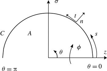
. The field and flow are assumed to be axisymmetric, which permits analytical integration of the integrands in (3.5), (3.6) and (3.8) over the azimuth, thus reducing the surface integrals to line integrals along the drop contour
 $C$
(see figure 2). Thus, the tangential coordinate
 $s$
corresponds to the continuous arclength along the surface of the drop measured from the positive
 $z$
-axis in the counterclockwise direction. The axisymmetric free-space Green’s functions
 $\boldsymbol{J}$
and
 $\boldsymbol{K}$
in (3.8) are computed in terms of elliptic integrals of the first and second kind respectively. These are extracted from the open-source library BEMLIB (Pozrikidis Reference Pozrikidis2010).
Computational diagram of the initial drop shape. As the field and flow are considered axisymmetric, the integral equations (3.5), (3.6) and (3.8) are reduced from integrals along the surface
 $A$
to integrals along the contour
 $C$
. Here, the normal
 $\boldsymbol{n}$
and tangential
 $\boldsymbol{t}$
vectors are illustrated; the former is positive when pointing outwards, while the latter is positive when pointing in the counterclockwise direction. Finally, the continuous arclength
 $s$
, which begins from the positive
 $z$
-axis (
 ${\it\theta}=0$
), is positive when pointing in the counterclockwise direction.

The top half of the drop (
 $0\leqslant {\it\theta}\leqslant {\rm\pi}$
) is partitioned into
 $N$
segments, typically ranging from
 $N=100$
to
 $200$
, for which all functions are interpolated by piecewise-continuous cubic polynomials (splines) parametrized with respect to the continuous arclength
 $s$
. Following Lac & Homsy (Reference Lac and Homsy2007), these polynomial representations may possess either vanishing first or second derivatives at the endpoints (
 ${\it\theta}=0,{\rm\pi}$
). Implementation of either one of these conditions for the unknown functions provides enough information to solve the boundary integral equations (3.5), (3.6) and (3.8). It should be noted that we do not assume symmetry with respect to the plane
 $z=0$
. Following standard regularization techniques (Pozrikidis Reference Pozrikidis2010), the logarithmically singular terms in these kernels are subtracted from the main integrals, thus rendering the integrands regular as the observer
 $\boldsymbol{y}$
approaches the source point
 $\boldsymbol{x}$
. Subsequently, the singularity is added back and integrated. The regular integrals in (3.5), (3.6) and (3.8) are then broken up into integrals along each segment, each of which is calculated by implementing Gauss–Legendre quadrature; the remaining singular integrals are computed by utilizing Gauss–Legendre quadrature for integrals that posses logarithmic singularities (Pozrikidis Reference Pozrikidis2010). All simulations are conducted until the normal velocity
 $u_{n,o}$
at every node is at most
 $O(10^{-4})$
, such that steady state is reached and no subsequent appreciable changes occur in the calculated quantities throughout time.
4. Computations for transient deformation
The impacts of charge relaxation and charge convection on transient drop deformation are first probed separately. Our focus is on the transient deformation; however, comparison of the attained steady state against values reported in the literature provides a useful check of our computations.
4.1. The effect of charge relaxation
We first examine the influence of the charging term
 $\partial q/\partial t$
in (3.10), while still focusing on the limit of negligibly small electric Reynolds numbers
 $\mathit{Re}_{i,o}\rightarrow 0$
. Here, convection of charge by the flow becomes negligible. In this limit, (3.10) yields the interfacial charging condition
 $$\begin{eqnarray}E_{n,i}-RE_{n,o}=R\frac{\partial q}{\partial t}.\end{eqnarray}$$
Here, the electrical relaxation time scales
 ${\it\tau}_{e(i,o)}={\it\varepsilon}_{i,o}{\it\chi}_{i,o}$
are considered to be non-zero, although small in comparison with the flow time scale
 ${\it\tau}_{f}=a/U$
. The interface acquires a surface charge
 $q$
over the time scales
 ${\it\tau}_{e(i,o)}$
, similar to the
 $RC$
time constant of a capacitor. It should be noted that although the convective term is neglected in (3.10), the effect of the electric Reynolds number
 $\mathit{Re}_{o}$
is preserved through the kinematic condition (3.12). This dimensionless group may be rewritten as
 $\mathit{Re}_{o}=\mathit{Ca}_{o}\,({\it\tau}_{e,o}/{\it\tau}_{c,o})$
, where
 ${\it\tau}_{c,o}={\it\mu}_{o}a/{\it\gamma}$
represents the capillary time scale based on the medium properties. Here,
 ${\it\tau}_{e,o}/{\it\tau}_{c,o}$
is the ratio of time scales
 ${\it\tau}_{e,o}/{\it\tau}_{p}$
defined by Saville (Reference Saville1997) which characterizes the transport of charge towards the interface, with the process time scale
 ${\it\tau}_{p}={\it\tau}_{c,o}$
. Hence, we label this ratio of time scales
 ${\it\tau}_{e,o}/{\it\tau}_{c,o}$
as a Saville number
 $\mathit{Sa}_{o}$
. To compare our computational results against published literature results for steady deformation, we focus on the particular set of dimensionless parameters
 $(S,M,R)=(20,1,0.5)$
, which was examined by Lac & Homsy (Reference Lac and Homsy2007), and corresponds to a drop that is less conductive than the medium and fluids that possess viscosities equal to one another. It should be noted that for this set of values (
 $SR>1$
), the steady-state conformation is oblate. The electric capillary number is held at
 $\mathit{Ca}_{o}=0.5$
. To probe the influence of a varying charging time scale
 ${\it\tau}_{e,o}$
, the transient deformation is examined as
 $\mathit{Sa}_{o}={\it\tau}_{e,o}/{\it\tau}_{c,o}$
is varied over two orders of magnitude.
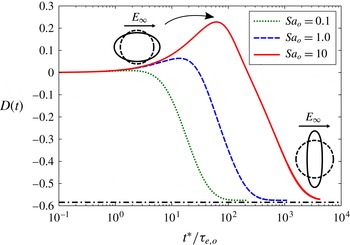
The transient deformation corresponding to
 $\mathit{Sa}_{o}=\{0.1,1,10\}$
and
 $\mathit{Ca}_{o}=0.5$
is illustrated in figure 3. All three curves achieve a steady deformation of
 $D=-0.58$
(denoted by the dash-dotted line), in agreement with Lac & Homsy (Reference Lac and Homsy2007). For this set of parameters, Taylor’s
 $O(\mathit{Ca})$
theory (1.1) would predict an oblate deformation
 $D_{T}$
of magnitude greater than unity, which is clearly incorrect. The fact that we approach the same steady-state value for the deformation as Lac and Homsy confirms that our numerical method has been implemented properly. Unlike Lac & Homsy (Reference Lac and Homsy2007), however, we also compute the entire transient deformation profile, which displays non-monotonic behaviour. In particular, an increasingly pronounced prolate–oblate shape transition is observed as
 $\mathit{Sa}_{o}$
increases. As described by Supeene et al. (Reference Supeene, Koch and Bhattacharjee2008) and Lanauze et al. (Reference Lanauze, Walker and Khair2013), an increasing charging time scale
 ${\it\tau}_{e,o}$
extends the amount of time for charge to reach the interface. Thus, at early times, both phases behave as perfect dielectrics; hence, the drop deforms along the applied field (prolate) due to the absence of sufficient induced electrohydrodynamic flow. Eventually, enough charge reaches the interface to drive the recirculatory flow and promote a change in configuration, thus yielding the expected ultimate oblate deformation. As
 $\mathit{Sa}_{o}$
is increased, the shape transition becomes more pronounced, in terms of the maximum transient prolate deformation; it also becomes more long-lived, in terms of the amount of time during which the shape remains prolate. It takes the solid curve describing
 $\mathit{Sa}_{o}=10$
more than an order of magnitude longer to reach steady state in comparison to the dotted curve corresponding to
 $\mathit{Sa}_{o}=0.1$
.
Transient deformation
 $D(t)$
as a function of dimensionless time for different ratios of charging
 ${\it\tau}_{e,o}$
to capillary
 ${\it\tau}_{c,o}$
time scales, which we label as a Saville number
 $\mathit{Sa}_{o}$
. The capillary number
 $\mathit{Ca}_{o}=0.5$
and the set of dimensionless parameters
 $(S,M,R)=(20,1,0.5)$
correspond to one of the cases analysed by Lac & Homsy (Reference Lac and Homsy2007). Here, time
 $t^{\ast }$
is normalized by the electrical relaxation time scale
 ${\it\tau}_{e,o}$
of the dotted curve describing
 $\mathit{Sa}_{o}=0.1$
. The shape of the drop possessing the largest transient prolate deformation (
 $\mathit{Sa}_{o}=10$
, the solid curve) and its steady oblate deformation shape (applicable to all three curves) are also shown. The dash-dotted line represents the steady state reported by Lac & Homsy (Reference Lac and Homsy2007).

4.2. The effect of charge convection
We now consider the effects of charge relaxation and charge convection. As a basis for comparison, we focus on a system for which
 $(S,M,R)=(0.5,1,100)$
, studied by Feng (Reference Feng1999). In figure 7 of that paper, Feng plots the steady deformation for this system as a function of the square of the applied dimensionless electric field, namely
 $E_{\infty }^{2}{\it\varepsilon}_{f}a/{\it\gamma}$
, where the field is normalized by performing a balance of electrical stress
 ${\it\varepsilon}_{f}E_{\infty }^{2}$
and interfacial stress
 ${\it\gamma}/a$
. Here,
 ${\it\varepsilon}_{f}$
is the permittivity of free space. In that figure, two curves, which correspond to zero and finite electric Reynolds number respectively, indicate that charge convection suppresses the steady oblate deformation at a given electric field strength. At an electric capillary number of
 $\mathit{Ca}_{o}=2$
(a dimensionless electric field squared of 0.4 in Feng’s paper), the simulation that does not consider charge convection is unable to predict a stable drop shape; the computation that is conducted at a non-zero electric Reynolds number
 $\mathit{Re}_{o}=0.7$
predicts a steady oblate conformation. It should be noted that our definition for
 $\mathit{Re}_{i,o}$
differs from that of Feng (Reference Feng1999). While we separately define an electric Reynolds number
 $\mathit{Re}={\it\varepsilon}{\it\chi}U/a$
for each phase, Feng defines this dimensionless group as
 $\mathit{Re}_{Feng}=({\it\varepsilon}_{i}+{\it\varepsilon}_{o}){\it\chi}_{i}{\it\chi}_{o}U_{Taylor}/({\it\chi}_{i}+{\it\chi}_{o})a$
, where
 $U_{Taylor}$
is expressed as the maximum interfacial angular velocity derived by Taylor (Reference Taylor1966).
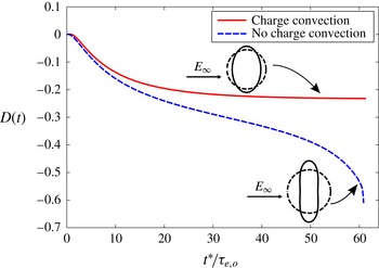
We predict exactly the same behaviour as Feng (Reference Feng1999) when comparing our simulations with and without charge convection. Additionally, we report the development towards the steady-state shape. Figure 4 depicts the transient deformation for these two conditions, where the dashed and solid curves correspond to computational results in the limit of electric Reynolds number
 $\mathit{Re}_{o}\rightarrow 0$
and
 $\mathit{Re}_{o}=0.7$
respectively. Although these two curves follow the same behaviour at early times (roughly
 $t=t^{\ast }/{\it\tau}_{e,o}<10$
), the dashed curve begins to diverge from the solid curve when
 $t\approx 10$
and finally predicts drop breakup, while the solid curve predicts a steady-state deformation of
 $D=-0.23$
(Feng Reference Feng1999). The fact that we achieve the same steady configuration as predicted by Feng indicates that proper numerical implementation of charge convection has been achieved. As described by Feng (Reference Feng1999), the stabilization of oblate drops due to charge convection results from the weakened tangential flow resulting from the distorted surface charge density profile, which we will discuss further below.
Transient deformation
 $D(t)$
as a function of dimensionless time
 $t=t^{\ast }/{\it\tau}_{e,o}$
. The capillary number
 $\mathit{Ca}_{o}=2$
and
 $(S,M,R)=(0.5,1,100)$
. Both curves account for charge relaxation (
 $\partial q/\partial t$
in (3.10)). The solid curve, however, results from a simulation that also includes charge convection (an electric Reynolds number of
 $\mathit{Re}_{o}=0.7$
), while the dashed curve is obtained in the limit
 $\mathit{Re}_{o}\rightarrow 0$
. Here, we display the final shape of the drop corresponding to the simulation conducted at finite
 $\mathit{Re}_{o}$
, which achieves a steady deformation. The shape resulting from the simulation carried out at
 $\mathit{Re}_{o}\rightarrow 0$
is shown right before the onset of numerical instability (
 $t\approx 60$
).

5. Comparison of computation against experiment
5.1. Experimental procedure
Two
 $5~\text{cm}\times 5~\text{cm}$
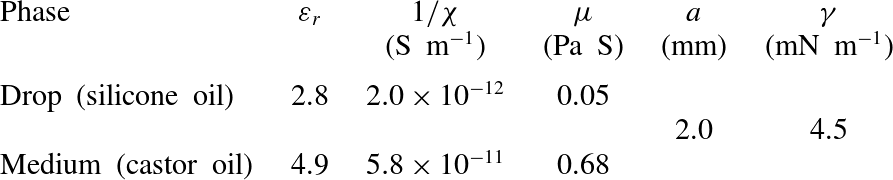
brass electrodes are attached to either side of a plastic cell, which holds the fluids, at a separation of 2 cm. A 1.9 cm diameter hole is made through the bottom of the cell to allow illumination with a fibre optic illuminator (Fiber-Lite MI-152, Dolan-Jenner Industries). A drop of silicone oil (Sigma-Aldrich) is injected into a castor oil (Sigma-Aldrich) medium from a
 $25~{\rm\mu}\text{l}$
glass syringe with a 22 gauge needle. A potential difference is applied across the two electrodes using a high-voltage power supply (Gamma High Voltage Research, Inc.). As soon as the field is applied, images are recorded at a rate of 15 f.p.s. with a firewire camera (Guppy PRO F-125B, Allied Vision Technologies) until the drop deformation reaches steady state. All image analyses are subsequently conducted with ImageJ software. Our experimental set-up is similar to that of Salipante & Vlahovska (Reference Salipante and Vlahovska2010).
To accurately predict the deformation of leaky dielectric systems, precise measurement of the fluid properties is crucial (Vizika & Saville Reference Vizika and Saville1992). Here, the permittivity
 ${\it\varepsilon}$
and resistivity
 ${\it\chi}$
of each phase are measured via electrochemical impedance spectroscopy (Yezer et al.
Reference Yezer, Khair, Sides and Prieve2014). The viscosity
 ${\it\mu}$
of each fluid is measured using a cone-and-plate rheometer (D-HR 2 rheometer, TA Instruments). Finally, the interfacial tension of the castor oil–silicone oil interface is extracted from the experimental work of Salipante & Vlahovska (Reference Salipante and Vlahovska2010). These material properties are listed in table 1. The greatest source of measurement error originates from the voltage measurement. For this purpose, a high-voltage probe (80K-15, Fluke Corporation) is implemented in conjunction with a standard digital multimeter (HHM29, Omega Engineering, Inc.). The error in measurement of the applied voltage is 2.25 % (based on the accuracy of the probe and multimeter). This error does not significantly change the results of any of our computational predictions. Given that we expect possible losses of voltage, we use the lower bound of the confidence in applied voltage in our computations. A minimum of six measurements of the transient drop deformation are taken per field strength. The transient deformation is then repeatedly measured for a different drop of approximately the same size and voltage to assess for reproducibility between different drops. All measurements produced similar results for the transient drop deformation. A representative measurement of deformation for each field strength at a fixed size is presented in this work to display the error in the deformation due to measurement of the drop semiaxes. It should be noted that we display this uncertainty because it is larger than the standard deviation that arises from the repeated measurement of the transient deformation.
Dimensional parameters for a silicone oil drop suspended in a castor oil medium. Here,
 ${\it\varepsilon}_{r}$
denotes the relative permittivity.

Dimensionless groups that describe a drop of silicone oil suspended in a castor oil medium at an electric field strength of
 $1.6~\text{kV}~\text{cm}^{-1}$
. See table 1 for dimensional quantities.

5.2. Transient deformation at an electric field strength of
 $1.6~\text{kV}~\text{cm}^{-1}$

The experimental castor oil–silicone oil system is described in table 1. For this set of parameters, all steady-state configurations are oblate. The corresponding dimensionless groups are listed in table 2. The viscosity ratio
 $M$
is less than unity; i.e. the drop is less viscous than the suspending medium. The capillary numbers
 $\mathit{Ca}_{i,o}$
are
 $O(10^{-1})$
, while the Saville numbers
 $\mathit{Sa}_{i,o}$
and electric Reynolds numbers
 $\mathit{Re}_{i,o}$
are greater than unity. Here,
 $\mathit{Sa}_{i,o}>1$
and
 $\mathit{Re}_{i,o}>1$
represent a dominance of the electrical relaxation time scales
 ${\it\tau}_{e(i,o)}$
over the capillary
 ${\it\tau}_{c(i,o)}={\it\mu}_{i,o}a/{\it\gamma}$
and flow
 ${\it\tau}_{f}=a/U$
time scales respectively. Thus, the transient and steady-state behaviour is controlled by the transport of charge towards and along the interface, i.e. we expect charge relaxation and charge convection to be relevant. The dimensionless groups in table 2 are implemented in our computations.
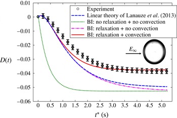
The experimental measurement of the deformation throughout time is depicted by the open circles in figure 5. The error bars in this curve originate from the measurement of the major
 $r_{2}^{\ast }$
and minor
 $r_{1}^{\ast }$
semiaxes, handled using standard propagation of error. The
 $O(\mathit{Ca})$
theory of Lanauze et al. (Reference Lanauze, Walker and Khair2013) which considers the charge relaxation
 ${\it\tau}_{e(i,o)}$
and momentum diffusion
 ${\it\tau}_{m(i,o)}=a^{2}{\it\rho}_{i,o}/{\it\mu}_{i,o}$
time scales is shown as the dashed curve. It should be noted that this theory yields the steady-state deformation
 $D_{T}$
(1.1) predicted by Taylor (Reference Taylor1966). Due to the fact that
 ${\it\tau}_{e(i,o)}\gg {\it\tau}_{m(i,o)}$
for this experimental system (assuming that
 ${\it\rho}_{o}={\it\rho}_{i}\approx 960~\text{kg}~\text{m}^{-3}$
), considering the momentum relaxation time scales
 ${\it\tau}_{m(i,o)}$
makes no difference in predicting the development of the drop shape; i.e. transient inertia is irrelevant and the flow is essentially quasi-steady. The theory captures the initial prolate–oblate shape transition during early times
 $t^{\ast }\lesssim 0.5~\text{s}$
, before diverging from the experimental measurement and overpredicting the steady deformation.
Transient deformation of a silicone oil drop suspended in a castor oil medium at a field strength of
 $1.6~\text{kV}~\text{cm}^{-1}$
. The dimensional parameters for this system are listed in table 1 and the dimensionless groups are listed in table 2. The open circles denote the experimental measurement, while the dashed curve illustrates the small-
 $\mathit{Ca}$
theory of Lanauze et al. (Reference Lanauze, Walker and Khair2013) which accounts for charge relaxation. The remaining curves result from boundary integral (BI) calculations. The dotted curve results from a simulation that considers an instantaneous interfacial charging with no charge convection, while the dash-dotted curve results from a simulation that considers finite electrical relaxation time scales
 ${\it\tau}_{e(i,o)}={\it\varepsilon}_{i,o}{\it\chi}_{i,o}$
with no charge convection. Finally, the solid curve results from a simulation that accounts for charge relaxation together with charge convection. The inset is an image of the steady oblate shape measured experimentally.

The remaining curves in figure 5 result from boundary integral calculations. The simulation that considers neither charge relaxation nor charge convection is implemented by making use of (4.1) and decreasing the resistivities
 ${\it\chi}_{i,o}$
by two orders of magnitude for use in (3.12), while still maintaining the resistivity ratio
 $R={\it\chi}_{i}/{\it\chi}_{o}$
unchanged. The result from this calculation is shown as the dotted curve in figure 5. This curve is unable to capture the shape transition, instead predicting a monotonic development towards a steady-state deformation that overpredicts the deformation measured in the experiment.
Dimensionless groups that describe a drop of silicone oil suspended in a castor oil medium at an electric field strength of
 $2.1~\text{kV}~\text{cm}^{-1}$
.

The dash-dotted curve in figure 5 results from a simulation that only takes charge relaxation into account through (4.1). This curve exhibits similar transient behaviour to the
 $O(\mathit{Ca})$
theory of Lanauze et al. (Reference Lanauze, Walker and Khair2013) during times
 $t^{\ast }\lesssim 2~\text{s}$
, which is unsurprising since they both account for charge relaxation (4.1). The dash-dotted curve eventually reaches the same steady state as the dotted curve that considers instantaneous charge relaxation and no charge convection. When the capillary number is not small, we expect the
 $O(\mathit{Ca})$
theory to deviate from this computational prediction (dash-dotted curve). It is merely a coincidence that the
 $O(\mathit{Ca})$
prediction is actually closer to the steady-state experimental measurement than the boundary integral calculation; the latter should provide a more accurate result at the capillary numbers
 $\mathit{Ca}_{i}=0.3$
and
 $\mathit{Ca}_{o}=0.5$
considered. The fact that this calculation is unable to capture the experimental curve together with the large electric Reynolds numbers
 $\mathit{Re}_{i,o}$
(table 2) leads us to consider the full charge-transport equation (3.10). The solid curve depicted in figure 5 results from a simulation that considers both charge relaxation and charge convection. Although slight deviation from the experiment is observed during intermediate times
 $0.5~\text{s}\lesssim t^{\ast }\lesssim 2.5~\text{s}$
, this computation provides a more accurate representation of the experimentally measured transient deformation (within the calculated error). Hence, both charge relaxation and charge convection in (3.10) must be accounted for when predicting time-dependent drop deformation for such low-conductivity systems with large electrical relaxation time scales
 ${\it\tau}_{e(i,o)}$
, such that
 $\mathit{Sa}_{i,o}>1$
and
 $\mathit{Re}_{i,o}>1$
. It should be noted that although the deformations illustrated in figure 5 are small, the nonlinear effect of charge convection still plays a role in determining the steady-state deformation. This is a central conclusion of our work.
5.3. Transient deformation at an electric field strength of
$2.1~\text{kV}~\text{cm}^{-1}$

The electric field is increased to
 $2.1~\text{kV}~\text{cm}^{-1}$
, yielding the dimensionless parameters in table 3. The electric capillary
 $\mathit{Ca}_{i,o}={\it\varepsilon}_{i,o}E_{\infty }^{2}a/{\it\gamma}$
and electric Reynolds
 $\mathit{Re}_{i,o}=E_{\infty }^{2}{\it\varepsilon}_{i,o}^{2}\,{\it\chi}_{i,o}/{\it\mu}_{i,o}$
numbers have increased due to their proportionality to
 $E_{\infty }^{2}$
, while the Saville numbers
 $\mathit{Sa}_{i,o}$
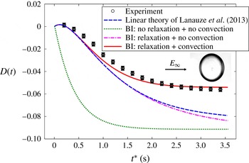
remain unchanged. The resulting experimental measurement and computational curves for this set of parameters are displayed in figure 6. The description for each of these curves is the same as in figure 5. Since larger capillary numbers
 $\mathit{Ca}_{i,o}$
are considered, the
 $O(\mathit{Ca})$
theory of Lanauze et al. (Reference Lanauze, Walker and Khair2013) shows a greater deviation at steady state from the boundary integral simulations and the experimental measurement. It should be noted that the dash-dotted curve (only charge relaxation) has not yet reached steady state in figure 6; it eventually settles towards the same steady deformation as the dotted curve (no charge relaxation or convection). Although the same trend is observed in the extent of agreement of the set of boundary integral calculations with the experimental measurement, the curves that are not able to capture the transient deformation profile measured in the experiment overpredict the steady-state deformation by a more substantial amount in comparison to figure 5. This is due to the more pronounced effect of charge convection, which is reflected through the increase in electric Reynolds numbers
 $\mathit{Re}_{i,o}$
due to the larger applied voltage.
Transient deformation of a silicone oil drop suspended in a castor oil medium at a field strength of
 $2.1~\text{kV}~\text{cm}^{-1}$
. The dimensional parameters for this system are listed in table 1 and the dimensionless groups are listed in table 3. The description of the curves is the same as in figure 5. The inset is an image of the steady oblate shape measured experimentally.

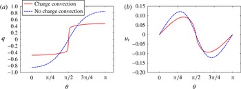
To understand why charge convection suppresses steady oblate deformations, we examine the surface charge density profile along the interface of the drop. Figure 7(a) shows the steady-state (
 $t^{\ast }\approx 3~\text{s}$
in figure 6) dimensionless interfacial charge
 $q$
as a function of the polar angle
 ${\it\theta}$
. As we assumed symmetry with respect to the azimuth
 ${\it\phi}$
(see figure 2), analysis of the results for the top half of the drop yields all necessary information to investigate the effects of surface charge convection. The dashed curve in figure 7(a) results from the simulation that does not take charge convection into account (4.1), while the solid curve considers the full governing equation (3.10) for charge transport. Here, the magnitude of the surface charge density
 $q$
is lessened throughout the regions away from the equator (
 ${\it\theta}={\rm\pi}/2$
) due to convection of charge from pole to equator. Convection of charge is also observed to cause a rapid variation in
 $q$
at the equator of the drop. As the scaling for the electrical stress is given by
 $[{\bf\tau}_{e}\boldsymbol{\cdot }\boldsymbol{n}]\sim qE_{\infty }$
, the pronounced reduction in
 $q$
leads to a decrease in the electrical stress. Due to the fact that oblate configurations are driven by an induced electrohydrodynamic flow, a simple balance of electrical and viscous stresses yields
 $U\sim qE_{\infty }a/{\it\mu}\sim {\it\varepsilon}E_{\infty }^{2}a/{\it\mu}$
. This relationship dictates that the decrease in
 $[{\bf\tau}_{e}\boldsymbol{\cdot }\boldsymbol{n}]$
provides a suppression of the flow strength
 $U$
that drives the deformation. This is illustrated in figure 7(b), where the tangential velocity
 $u_{t,o}=u_{t,i}=\boldsymbol{u}_{i,o}\boldsymbol{\cdot }\boldsymbol{t}$
is presented as a function of the polar angle
 ${\it\theta}$
for the cases where charge convection is considered (solid line) and neglected (dashed line). Here, a weakening of the tangential flow is present throughout the regions of reduced interfacial charge
 $q$
. This reasoning helps us to understand the difference between the simulated steady deformations that do and do not account for surface convection of charge in figure 6. It should be noted that the magnitude of the steady-state charge
 $\int _{S}q\,\text{d}S=\int _{C}2{\rm\pi}q{\it\sigma}\,\text{d}C$
that resides on each half of the drop decreases with increasing electric Reynolds numbers
 $\mathit{Re}_{i,o}$
. When charge convection is accounted for, charge swept from pole to equator by the induced electrohydrodynamic flow is neutralized at the equator. Hence, the overall amount of charge on each half of the drop is reduced.
(a) Steady interfacial charge density profile
 $q$
as a function of the polar angle
 ${\it\theta}$
corresponding to a silicone oil drop suspended in a castor oil medium at a field strength of
 $2.1~\text{kV}~\text{cm}^{-1}$
(
 $t^{\ast }\approx 3~\text{s}$
in figure 6). The solid curve results from the simulation that considers surface charge convection from the poles (
 ${\it\theta}=0,{\rm\pi}$
) towards the equator (
 ${\it\theta}={\rm\pi}/2$
) of the drop; the dashed curve does not account for interfacial charge convection. (b) Steady interfacial tangential velocity
 $u_{t}$
(note that
 $u_{t,o}=u_{t,i}$
) as a function of the polar angle
 ${\it\theta}$
(
 $t^{\ast }\approx 3~\text{s}$
in figure 6). The solid curve results from the simulation that considers surface charge convection towards the equator of the drop; the dashed curve does not account for interfacial charge convection.

We now examine the development of the two steady surface charge density profiles
 $q$
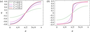
displayed in figure 7(a). Figure 8(a) illustrates the evolution of interfacial charge that yields the steady state depicted by the dashed curve in figure 7(a), while figure 8(b) illustrates the evolution of interfacial charge that yields the steady state depicted by the solid curve in figure 7(a). In figure 8(a), the four curves present a gradual development towards the steady charge density profile. Here, all curves qualitatively display a
 $\cos ({\it\theta})$
dependence that results due to charge accumulating at the interface without any convection by the fluid flow. If convection of charge by the induced electrohydrodynamic flow is accounted for, the flow sweeps the accumulating charge from pole to equator (figure 8
b). Here, the maximum in surface charge
 $q$
increases at the poles as time progresses. Simultaneously, the previously described sharp variation in
 $q$
occurs at the equator due to charge convection from pole to equator. As the electric Reynolds numbers
 $\mathit{Re}_{i,o}$
increase at high electric field strengths, the governing equation for interfacial charge (3.10) becomes approximately hyperbolic. Thus, there exists the possibility of a ‘charge shock’, in which the surface charge distribution displays nearly discontinuous behaviour at the equator, as illustrated in figure 8(b) for
 $t^{\ast }=3~\text{s}$
.
Development of the interfacial charge density profile
 $q$
as a function of the polar angle
 ${\it\theta}$
for a silicone oil drop suspended in a castor oil medium at a field strength of
 $2.1~\text{kV}~\text{cm}^{-1}$
. (a) The set of curves corresponds to the simulation for transient deformation that accounts for charge relaxation and does not consider charge convection in figure 6 (the dash-dotted curve), which eventually yields the same steady-state surface charge density distribution as the dashed curve in figure 7(a). (b) The set of curves corresponds to the simulation for transient deformation that accounts for both charge relaxation and charge convection in figure 6 (the solid curve), which eventually yields the same steady-state surface charge density distribution as the solid curve figure 7(a).

5.4. Transient deformation at an electric field strength of
$6.1~\text{kV}~\text{cm}^{-1}$

The electric field is further increased to
 $6.1~\text{kV}~\text{cm}^{-1}$
, which provides the dimensionless groups listed in table 4. The electric capillary
 $\mathit{Ca}_{i,o}$
and electric Reynolds
 $\mathit{Re}_{i,o}$
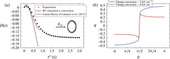
numbers have increased by approximately an order of magnitude in comparison with table 3. The results for this system are presented in figure 9(a,b). In figure 9(a), only the experimental measurement of the transient deformation, the boundary integral simulation that considers charge relaxation and charge convection through (3.10), and the
 $O(\mathit{Ca})$
theory of Lanauze et al. (Reference Lanauze, Walker and Khair2013) are displayed. Although the deformation in the experiment reaches steady state at approximately time
 $t^{\ast }\approx 3~\text{s}$
, the simulation only reaches
 $t^{\ast }\approx 0.8~\text{s}$
, at which time the normal velocity
 $u_{n,o}$
in (3.12) is
 $O(10^{-3})$
. The computation is only shown until this point in time. From this point forth
 $u_{n,o}$
increases, eventually predicting an unstable drop conformation. The
 $O(\mathit{Ca})$
theory is displayed until
 $t^{\ast }\approx 0.75~\text{s}$
as a basis for comparison against the other curves. The curve corresponding to the linear theory begins to deviate from the computation and experiment at approximately
 $D=-0.02$
, and ends with a large overprediction of the steady deformation measured experimentally (
 $D_{T}=-0.72$
, not shown).
Dimensionless groups that describe a drop of silicone oil suspended in a castor oil medium at an electric field strength of
 $6.1~\text{kV}~\text{cm}^{-1}$
.

(a) Transient deformation of a silicone oil drop suspended in a castor oil medium at a field strength of
 $6.1~\text{kV}~\text{cm}^{-1}$
. The dimensional parameters for this system are listed in table 1 and the dimensionless groups are listed in table 4. The open circles denote the experiment, while the dashed curve illustrates the small-
 $\mathit{Ca}$
theory of Lanauze et al. (Reference Lanauze, Walker and Khair2013) that considers charge relaxation. Finally, the solid line represents the boundary integral simulation that accounts for both charge relaxation and charge convection through (3.10). The inset is an image of the steady oblate shape measured experimentally. (b) Interfacial charge density profile
 $q$
as a function of the polar angle
 ${\it\theta}$
. The solid curve results from the simulation corresponding to a field strength of
 $6.1~\text{kV}~\text{cm}^{-1}$
(
 $t^{\ast }\approx 0.8~\text{s}$
in figure 9
a), which considers surface charge convection from the poles (
 ${\it\theta}=0,{\rm\pi}$
) towards the equator (
 ${\it\theta}={\rm\pi}/2$
) of the drop. The dashed curve accounts for charge convection at a field strength of
 $2.1~\text{kV}~\text{cm}^{-1}$
, which results in a steady-state profile (note that this is the same curve as the solid curve in figure 7
a).

The surface charge density
 $q$
as a function of the polar angle
 ${\it\theta}$
corresponding to the approximate point of instability of the computation,
 $t^{\ast }\approx 0.8~\text{s}$
in figure 9(a), is illustrated through the solid curve in figure 9(b). The dashed curve is exactly the same as the solid curve in figure 7(a), which considers charge convection and is able to predict the steady-state deformation displayed by the solid curve in figure 6 at a lower field strength of
 $2.1~\text{kV}~\text{cm}^{-1}$
. Although a sharp variation in
 $q$
was previously observed in figure 7(a) at the equator of the drop at a field of
 $2.1~\text{kV}~\text{cm}^{-1}$
due to interfacial charge convection directed from pole to equator, this abrupt change is further accentuated when the field is increased to
 $6.1~\text{kV}~\text{cm}^{-1}$
. Furthermore, this increase in field strength provides a maximum in the magnitude of the interfacial charge distribution
 $q$
near the equator, thus providing a non-monotonic surface charge density profile. If the simulation were to proceed beyond
 $t^{\ast }\approx 0.8~\text{s}$
, the sharp variation at the equator and the maximum in
 $q$
would both increase until the curve ceased to be smooth and the simulation terminated.
We believe that the solid curve in figure 9(b) is an artefact of the imposed axisymmetry of the boundary integral calculation. At a high enough electric field strength, an onset of drop rotation and three-dimensional flow is expected due to an electric torque exerted to restore the misaligned dipole that arises in systems for which
 ${\it\tau}_{e,i}>{\it\tau}_{e,o}$
(Ha & Yang Reference Ha and Yang2000b
; Salipante & Vlahovska Reference Salipante and Vlahovska2010). Hence, axisymmetric oblate deformations are unstable to three-dimensional instabilities at high electric fields (Saville Reference Saville1997). This phenomenon is akin to Quincke rotation for a solid particle suspended in a fluid (Quincke Reference Quincke1896). To check whether this critical voltage for the onset of rotation has been reached, we calculate the threshold electric field for a solid particle (Jones Reference Jones1984),
 $$\begin{eqnarray}E_{Q}=\sqrt{\frac{2{\it\mu}_{o}S(2R+1)^{2}}{3{\it\varepsilon}_{i}{\it\varepsilon}_{o}{\it\chi}_{o}R(RS-1)}},\end{eqnarray}$$
where
 $E_{Q}$
denotes the critical electric field for the onset of Quincke rotation of a solid particle. Equation (5.1) is obtained by balancing the electrical and viscous torques on a spherical rigid object. It is independent of particle size since both the electrical and viscous torques scale as
 $a^{3}$
. We implement this expression as an approximation; considerable experimental deviation from (5.1) has been observed for low-viscosity drops (Ha & Yang Reference Ha and Yang2000b
; Salipante & Vlahovska Reference Salipante and Vlahovska2010), which is the regime of our experiments (
 $M=0.1$
). Insertion of the dimensional parameters from table 1 and the dimensionless groups
 $S,M,R$
from table 2 yields
 $E_{Q}=3.2~\text{kV}~\text{cm}^{-1}$
. For our system, the experimental onset of rotation occurs at a threshold field strength of approximately
 $6.8~\text{kV}~\text{cm}^{-1}$
– only
 $0.7~\text{kV}~\text{cm}^{-1}$
greater than the field strength in figure 9 – which is closer to the threshold electric fields reported in the literature (Ha & Yang Reference Ha and Yang2000b
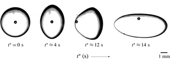
; Salipante & Vlahovska Reference Salipante and Vlahovska2010) for castor oil–silicone oil systems. As illustrated in figure 10, such three-dimensional instabilities may occur for deformations of modest amplitude. Here, the sequential images illustrate the silicone oil drop acquiring an oblate shape and then transitioning towards an unstable configuration.
Onset of rotation and three-dimensional flow of a silicone oil drop suspended in a castor oil medium at a field strength of
 $6.8~\text{kV}~\text{cm}^{-1}$
. An air bubble is present inside the drop. This bubble does not affect the experimental measurement; it allows the direction of flow to be traced.

6. Conclusion
We have analysed the nonlinear transient deformation of a leaky dielectric drop of permittivity
 ${\it\varepsilon}_{i}$
, resistivity
 ${\it\chi}_{i}$
and viscosity
 ${\it\mu}_{i}$
suspended in a medium with permittivity
 ${\it\varepsilon}_{o}$
, resistivity
 ${\it\chi}_{o}$
and viscosity
 ${\it\mu}_{o}$
. Our first contribution was the calculation of the transient deformation via an axisymmetric boundary integral method, which accounts for surface charge convection and a finite relaxation time scale for interfacial accumulation of charge. For steady oblate drops, the dominant electrical relaxation time scales
 ${\it\tau}_{e(i,o)}={\it\varepsilon}_{i,o}{\it\chi}_{i,o}$
yielded an initial prolate configuration due to a lack of sufficient charge at the interface (Supeene et al.
Reference Supeene, Koch and Bhattacharjee2008; Lanauze et al.
Reference Lanauze, Walker and Khair2013), which in turn caused the drop and medium to initially behave akin to perfect dielectrics. As the ratio of charge relaxation to capillary time scale (Saville number
 $\mathit{Sa}_{o}={\it\tau}_{e,o}/{\it\tau}_{c,o}$
) increased at a fixed capillary number
 $\mathit{Ca}_{o}$
, the prolate conformation became more pronounced and long-lived, while the steady-state deformation remained unchanged. Furthermore, charge convection was shown to restrain steady oblate deformations.
Our second contribution was a direct comparison of numerical simulation against experimental measurement with no adjustable parameters. Our focus on oblate drops was due to their flow-driven nature, which therefore accentuates interfacial charge convection (Feng Reference Feng1999). Both charge relaxation and charge convection were required to correctly quantify the time-dependent deformations measured experimentally. Furthermore, these two forms of surface charge transport were found to operate simultaneously rather than serially (see figure 8
b); that is, charge accumulates at the interface as the electrohydrodynamic flow convects the charge from pole to equator. Good agreement was observed for moderate electric field strengths (
 $1.6~\text{kV}~\text{cm}^{-1}$
,
 $2.1~\text{kV}~\text{cm}^{-1}$
). However, the computation failed as the field increased towards
 $6.1~\text{kV}~\text{cm}^{-1}$
, which was due to an onset of drop rotation and unsteady three-dimensional flow (Ha & Yang Reference Ha and Yang2000b
; Salipante & Vlahovska Reference Salipante and Vlahovska2010). Although the oblate deformations illustrated in figures 5 and 6 were moderate, charge convection provided a strong nonlinear effect on the interfacial charge distribution
 $q$
, as illustrated in figures 7(a) and 9(b). We have not encountered such distorted surface charge density profiles in published works that consider the effects of interfacial charge convection on steady oblate electrohydrodynamic drop deformation (Feng Reference Feng1999; Fernández Reference Fernández2013), which we believe is due to the lack of any reported results at such high electric Reynolds numbers,
 $\mathit{Re}_{i,o}={\it\tau}_{e(i,o)}/{\it\tau}_{f}$
. This effect, which mostly reduced
 $q$
throughout the interface, translates to a less-pronounced tangential flow
 $u_{t}$
(figure 7
b), and thus a reduced oblate deformation. Thus, the modest deformations measured experimentally required a nonlinear model to enable an accurate prediction.
Our boundary integral calculations enabled the prediction of the transient deformation of the castor oil–silicone oil system in tables 2 and 3; however, room for improvement of the experimental set-up exists. The most substantial issue in our system is the dielectrophoretic migration of silicone oil drops at high electric field strengths. Although care was taken when injecting the drop into the centre of the cell, we believe that more careful alignment of the electrodes would minimize the migration of these drops, and improve agreement between our computations and the experiments in figures 5 and 6. Our work emphasizes the need to consider both charge relaxation and charge convection when modelling the transient deformation of leaky dielectric systems at large Saville
 $\mathit{Sa}_{i,o}$
and electric Reynolds
 $\mathit{Re}_{i,o}$
numbers. The significant effects of these two phenomena serve as motivation to perform further experimental and computational studies that consider a wider range of systems with differing permittivity
 $S$
, resistivity
 $R$
and viscosity
 $M$
ratios. Finally, a fully three-dimensional boundary integral simulation would prove useful in predicting steady-state drop deformation at higher electric fields, as well as the exact field strength at the onset of drop rotation and unsteady flow observed in experiments (Ha & Yang Reference Ha and Yang2000b
; Salipante & Vlahovska Reference Salipante and Vlahovska2010).
Acknowledgements
We are grateful to P. Vlahovska, P. Salipante, E. Lac, A. Ramchandran and M. Loewenberg for rewarding discussions regarding experiments and computations. We also thank B. Yezer for performing electrochemical impedance spectroscopy measurements. Finally, we thank the National Science Foundation for support through grant number CBET-1066853.