
 L1





Nomenclature
-
 $d$
-
one of the shade-fixed principal axes in a direction normal to the axis of symmetry
-
$F$
-
force
-
$G$
-
universal gravitational constant
-
$I$
-
crosswise moment of inertia of the shade
-
${I}_{o}$
-
symmetry axis moment of inertia of the shade
-
$k$
-
constant associated with solar radiation pressure
-
$m$
-
mass of the shade
-
${M}_{E}$
-
mass of the Earth
-
${M}_{S}$
-
mass of the Sun
-
$o$
-
shade-fixed principal axis along the shade’s axis of symmetry
-
${o}_{B}$
-
height of the shade centre of mass above the apex
-
$q$
-
one of the shade-fixed principal axes running perpendicular to the axis of symmetry
-
$R$
-
radius of the shade
-
${r}_{E}$
-
distance from the Sun to the Earth
-
$x$
-
space-fixed axis running from the Sun to the Earth
-
$y$
-
space-fixed axis perpendicular to
$x$
and
$z$
-
$z$
-
space-fixed axis along the angular velocity of Earth in its rotation about the Sun
-
$\alpha $
-
parameter determining the curvature of the shade
-
$\varphi $
-
Euler angle to prescribe the orientation of the shade
-
$\theta $
-
Euler angle to prescribe the orientation of the shade
-
$\psi $
-
Euler angle to prescribe the orientation of the shade
-
$\sigma $
-
surface density of the shade
-
$\tau $
-
torque
-
$\mathrm{\Omega }$
-
angular velocity of Earth about Sun


1.0 Introduction
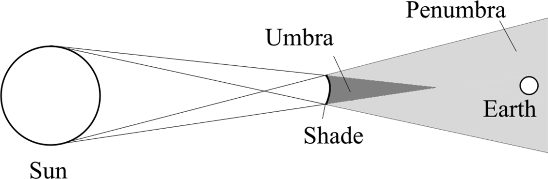
Unprecedented heat waves, melting of polar ice caps, drought and flooding conditions, as well as wildfires, have been attributed to climate change (e.g. Refs [Reference Shahgedanova and Letcher1, Reference Wehner, Arnold, Knutson, Kunkel and LeGrande2]). No part of the world has been spared the adverse effects. A multi-pronged strategy is required to mitigate the escalating impacts of climatic warming [3]. One mitigation approach consists of space-based solar shading, in which a gigantic shade is mounted in space to physically reduce the amount of solar radiation reaching the Earth’s surface. Through this option, an immediate (following deployment) and controlled reduction in insolation (incoming solar radiation) can be achieved on the Earth’s surface. Hence, one can mitigate global warming, while longer-term solutions are still under construction. A schematic representation of such a shade is shown in Fig. 1.
Schematic representation of the shade between the Sun and the Earth. The dimensions as well as distances are not to scale. Umbra and penumbra are shown.

The concept of a gigantic shade mounted in space was first proposed by Early [Reference Early4]. The idea featured a huge disk mounted at
 ${L}_{1}$
, the first Sun-Earth Lagrange point. Other early adherents of the concept include Mautner [Reference Mautner5], Govindasamy and Calderia [Reference Govindasamy and Calderia6] and Angel [Reference Angel7]. Among these, Mautner [Reference Mautner5] was in favour of a belt of reflective material in low-earth orbit, similar to Saturn’s rings. Govindasamy and Calderia [Reference Govindasamy and Calderia6] have considered both the Early and Mautner proposals, as well as others, highlighting the advantages and challenges associated with each. Angel [Reference Angel7] has proposed a cluster of innumerable small spacecraft at
 ${L}_{1}$
. It is noted that
 ${L}_{1}$
and the second Sun-Earth Lagrange point
 ${L}_{2}$
on the other side of the Earth are saddle points, which are unstable equilibrium points (see, e.g. Refs [Reference Cacolici, Hanson, Lejoly and Pearson8, Reference Muralidharan9]). Spacecraft in orbital motions about these Lagrange points, such as the James Webb telescope about the
 ${L}_{2}$
point and the Aditya
 ${L}_{1}$
probe of the Indian Space Research Organization about the
 ${L}_{1}$
point, need to use hydrazine thrusters to keep the spacecraft in position.
More recently, Sanchez and McInnes [Reference Sanchez and McInnes10] have performed a detailed analysis of orbiting configurations of occulting disks, which not only achieve a given reduction in incident solar energy, but also seek to minimise regional differences in impact. They have considered the effect of solar radiation pressure (SRP) acting on the shade and have shown that the equilibrium point is displaced to the Sun from
 ${L}_{1}$
. Given the density of the shade material, these authors have calculated the mass of shade required to obtain a given reduction in insolation at different points between the
 ${L}_{1}$
point and the Sun. They have found a minimum at a point approximately 50% farther away from Earth than the
 ${L}_{1}$
point. Borgue and Hein [Reference Borgue and Hein11] proposed a different kind of shade, which is based on refraction rather than reflection of sunlight. The absence of reflection results in zero radiation pressure on the shade. Hence, there is no mass requirement to ensure a location close to
 ${L}_{1}$
. Consequently, the shade can be made extremely light, and the cost of deployment is drastically reduced as compared to an occluding shade. However, the absence of SRP can be limiting in terms of both mobility and stability. Roy [Reference Roy12] has discussed the current status, along with future shade possibilities.
The use of SRP to achieve non-Keplerian orbits was first demonstrated by McInnes et al. [Reference Ceriotti and McInnes13, Reference Heiligers, Ceriotti, McInnes and Biggs14]. In these papers, pole-sitter orbits as well as displaced geostationary orbits are considered. These orbits are made feasible through the use of a combination of propellant, solar sail and solar electric propulsion thrusters. Soldini et al. [Reference Soldini, Colombo and Walker15] considered the use of these sails to facilitate the disposal of spacecraft in orbits of libration. Their strategy consists of moving the spacecraft to the unstable manifold of the libration orbit and then deploying the solar sail to increase the spacecraft’s energy and ensure its permanent separation from the Earth. Continuous regulation of the size and orientation of the solar sail has been suggested to utilise radiation pressure to achieve more complicated manoeuvres. Soldini et al. [Reference Soldini, Colombo and Walker15] have further shown how SRP can be used to achieve a transfer between two Lissajous orbits. Farres et al. [Reference Farres, Heiligers and Miguel16] have demonstrated the use of radiation pressure to transfer a spacecraft from the
 ${L}_{1}$
point to the remote
 ${L}_{4}$
and
 ${L}_{5}$
points. This has been extended by Fuglesang and Miciano [Reference Fuglesang and Miciano17] to achieve transfer of a solar sail from the Earth to the
 ${L}_{1}$
point. Sliding mode control has been used to design a trajectory starting from a low Earth orbit and ending at the
 ${L}_{1}$
point with zero speed.
With regard to the shape changing algorithm, Ceriotti et al. [Reference Ceriotti, Harkness, McRobb and Macdonald18] have shown that an adjustable quasi-rhombic pyramidal-shaped solar sail with bevel crux drive can enable management of the direction and magnitude of the thrust of the solar sail without resorting to propellant, control masses or variable-transmissibility materials. The geometry proposed by these authors [Reference Ceriotti, Harkness, McRobb and Macdonald18] is heliostable, in the sense that the torque on the sail always tends to orient it along a sun-facing direction. On the other hand, Ma et al. [Reference Ma, Murray and Munday19] have considered the problem of steering a solar sail by tunable radiation pressure. These authors propose a solar sail concept made of aluminium with polymer dispersed liquid crystal (PDLC) devices deployed along the periphery. PDLCs can be configured to allow light to pass through virtually unimpeded or to scatter it in forward as well as backward directions. There is no momentum transfer in the former case but positive transfer in the latter case, and this force is harnessed to achieve a torque and thereby a change in orientation of the solar sail. A different shape-changing algorithm has been considered by Russo et al. [Reference Russo, Robb, Soldini, Paoletti, Bailet, McInnes, Reveles, Sugihara, Bonardi and Mori20]. They consider an origami-inspired solar sail structure containing variable-reflectivity material. It is shown that by changing the reflectivity of the sail in some locations, origami folding and/or unfolding can be triggered, and the process can occur spontaneously thereafter. Further details of this can be found in the work of Robb et al. [Reference Robb, Russo, Soldini, Paoletti, Reveles, Bailet and McInnes21].
In the present work, the authors consider the paraboloidal shade at the Lagrange point
 ${L}_{1}$
, study the stability of the shade and propose a shape-changing control scheme. This work is a follow-up to the work presented in an invention disclosure [Reference Balachandran, Severinsky and Shayak22] and a conference presentation [Reference Shayak and Balachandran23]. The remainder of the paper is organised as follows. In Section 2, the model and setup are presented. In Section 3, the stability of the shade is considered, and the criteria for stability of translational and rotational modes are determined. In Section 4, the shade control architecture is discussed briefly, followed by brief discussions on a few stabilisation aspects. Limitations and practical feasibility of the proposed shade are then discussed in Section 5. The paper is concluded with a brief coda in Section 6.
2.0 Shade at the
$L_{1}$
point: system model and setup

In this section, the model is set up for the calculations that will follow. As an extended body, the shade is subject to different forces on the different component parts as a result of the Earth’s gravity field, the Sun’s gravity field, SRP and centrifugal and Coriolis forces. Due to these spatially heterogeneous forces, torques are also exerted about the centre of mass (CoM). It is desired to calculate the resultant forces and torques on the shade given the location in space of its apex. In particular, locations on the Earth-Sun axis near the Lagrange point
 ${L}_{1}$
will be of interest.
2.1 Geometry and coordinates
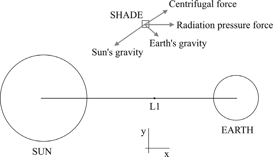
As shown in Fig. 2, let
 $x,y,z$
be directed along a set of dextral, orthogonal axes fixed in the reference frame centred at the Sun-Earth barycentre and rotating with the Earth. For all practical purposes, the origin may be taken as the centre of the Sun. The
 $x$
-axis is directed from the Sun to the Earth, the
 $z$
-axis is along the rotational angular velocity direction and the
 $y$
-axis is directed along the mutual perpendicular direction.
Schematic diagram of the Sun, the Earth and the shade for showing the axis convention and the frame of reference. The shade is shown as a point for clarity. The figure is not to scale.

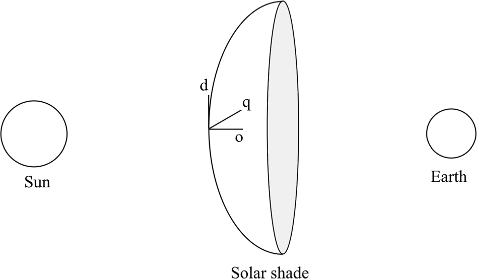
The shade is assumed to be a paraboloid of revolution and
 $q,d,o$
are associated with the shade’s principal axes with the origin at the apex and
 $o$
being associated with the axis of symmetry. The shade is treated as a surface; that is, a body of zero thickness. A schematic version is shown in Fig. 3. The equation for the shade surface takes the form
 \begin{align}o=\alpha \left({q}^{2}+{d}^{2}\right)\end{align}
where
 $\alpha $
is the curvature parameter. Let the shade have a radius
 $R$
so that it exists in the region
 \begin{align}{q}^{2}+{d}^{2}\le {R}^{2}\end{align}
The shade. It is shown as opening outwards from the Sun since that is essential for stability, as will be demonstrated later. This figure is not to scale.

An integration can be used to show that the CoM lies at the point
 $(\mathrm{0,0},{o}_{B})$
where
 \begin{align}{o}_{B}=\frac{{\big(4{\alpha }^{2}{R}^{2}+1\big)}^{3/2}\left(6{\alpha }^{2}{R}^{2}-1\right)+1}{10\alpha \left[{\left(4{\alpha }^{2}{R}^{2}+1\right)}^{3/2}-1\right]}\end{align}
In the limit of small
 $\alpha $
, when the shade is reduced to a disk, one finds
 \begin{align}{o}_{B}=\frac{\alpha {R}^{2}}{2}\end{align}
Any point on the shade is uniquely identified by the two coordinates
 $q,d$
. The infinitesimal area element at point
 $(q,d)$
is given by
 \begin{align}\mathrm{d}A=\sqrt{4{\alpha }^{2}{q}^{2}+4{\alpha }^{2}{d}^{2}+1}\mathrm{d}q\mathrm{d}d\end{align}
Let the surface density – that is, mass per unit area of the material – be
 $\sigma $
so that the infinitesimal mass element is
 \begin{align}\mathrm{d}m=\sigma \sqrt{4{\alpha }^{2}{q}^{2}+4{\alpha }^{2}{d}^{2}+1}\mathrm{d}q\mathrm{d}d\end{align}
The reference configuration of the shade features the apex (origin of the qdo basis) at the point
 $({x}_{0},\mathrm{0,0})$
where
 ${x}_{0}$
is determined from the equilibrium force balance. Furthermore, the
 $o$
-axis of the shade is coincident with the
 $x$
-axis so that
 $o,q,d$
correspond to
 $x,y,z$
in the reference configuration (the shade is chosen to open out away from the Sun). In the displaced configuration, the apex is translated by distances
 ${\eta }_{x}$
,
 ${\eta }_{y}$
, and
 ${\eta }_{z}$
along the three axes. Further, to model the angular perturbations, the shade is rotated first through angle
 $\varphi $
about the
 $y$
-axis, then through angle
 $\theta $
about the new
 $z$
-axis and finally through angle
 $\psi $
about the new
 $x$
-axis (shade axis of symmetry).
2.2 Structure of the equations of motion
The translational equations of motion of the shade are given by
 \begin{align}\begin{array}{ll}m{\ddot{\eta }}_{x} {} ={F}_{x}\\[3pt] m{\ddot{\eta }}_{y} {} ={F}_{y}\\[3pt] m{\ddot{\eta }}_{z} {} ={F}_{z}\end{array}\end{align}
where
 $m$
is the mass of the shade and
 ${F}_{x,y,z}$
are the resultant forces along the three fundamental directions. At this step, the displacements
 ${\eta }_{x}$
,
 ${\eta }_{y}$
and
 ${\eta }_{z}$
can be arbitrary, although they will be assumed to be small in magnitude later on.
The rotational dynamics of the shade are given by Euler’s equations, with the angular velocity being related to the Euler angle derivatives through the usual Tait–Bryan conventions [Reference Greenwood24]. The angular momentum balance equations are given by
 \begin{align}\begin{array}{ll} {} {I}_{q}{\dot{\omega }}_{q}+({I}_{o}-{I}_{d}){\omega }_{o}{\omega }_{d}={\tau }_{q}\\[3pt] {} {I}_{d}{\dot{\omega }}_{d}+({I}_{q}-{I}_{o}){\omega }_{q}{\omega }_{o}={\tau }_{d}\\[3pt] {} {I}_{o}{\dot{\omega }}_{o}+({I}_{d}-{I}_{q}){\omega }_{d}{\omega }_{q}={\tau }_{o}\end{array}\end{align}
with
 $\tau $
used to denote the torque and the angular velocity being given by
 \begin{align}\omega =\big(\dot{\theta }\,\mathrm{sin}\,\varphi +\dot{\psi }\,\mathrm{cos}\,\theta\, \mathrm{cos}\,\varphi \big){\hat{\mathbf{n}}}_{x}+\big(\dot{\varphi }+\dot{\psi }\,\mathrm{sin}\,\theta \big){\hat{\mathbf{n}}}_{y}+\big(\dot{\theta }\,\mathrm{cos}\,\varphi -\dot{\psi }\,\mathrm{cos}\,\theta \,\mathrm{sin}\,\varphi \big){\hat{\mathbf{n}}}_{z}\end{align}
where the orthogonal set of unit vectors
 ${\hat{\mathbf{n}}}_{x}$
,
 ${\hat{\mathbf{n}}}_{y}$
and
 ${\hat{\mathbf{n}}}_{z}$
are fixed at the shade centre. When the angles and angular velocities are small in magnitude, these equations can be simplified considerably. Since only small perturbations of the angles from the reference configuration are realistic in this problem, this assumption is immediately made. Then, the gyroscopic coupling terms in Euler’s equations disappear, and one is left with
 \begin{align}{I}_{o}{\dot{\omega }}_{o} {} &={\tau }_{o}\nonumber\\[3pt] I{\dot{\omega }}_{q} {} &={\tau }_{q}\\[3pt] I{\dot{\omega }}_{d} {} &={\tau }_{d}\nonumber\end{align}
where the moments of inertia
 ${I}_{q}$
and
 ${I}_{d}$
are related as
 ${I}_{q}={I}_{d}=I$
from symmetry. Due to the perfect symmetry of the shade, the angle
 $\psi $
does not influence the dynamics of
 $\varphi $
and
 $\theta $
. Hence, it can be assumed that
 $\psi =0$
throughout. For any vector
 $\mathbf{V}$
, the associated components can be transformed from the
 $xyz$
basis to the
 $oqd$
basis as per the rotation matrix
 \begin{align}\left[\begin{array}{l}{V}_{o}\\ {V}_{q}\\ {V}_{d}\\ \end{array}\right]={\mathbf{R}}_{xy}^{oqd}\left[\begin{array}{l}{V}_{x}\\ {V}_{y}\\ {V}_{z}\\ \end{array}\right]\end{align}
where
 \begin{align}{\mathbf{R}}_{xyz}^{oqd}=\left[\begin{array}{c@{\quad}c@{\quad}c}1& \theta& -\varphi \\ -\theta & 1& 0\\ \varphi& 0& 1\end{array}\right]\end{align}
This matrix is orthogonal up to
 $O(\varphi ,\theta )$
and is antisymmetric. By using this matrix, one can resolve the angular derivatives to form the angular velocity vector.
 $\dot{\varphi }$
, which is about the
 $y$
-axis, can be resolved into the
 $oqd$
bases as
 $\dot{\varphi }\left(\theta {\hat{\mathbf{n}}}_{o}+{\hat{\mathbf{n}}}_{q}\right)$
. After neglecting the second-order term, this vector can be treated as being directed about the
 $q$
-axis.
 $\dot{\theta },$
on the other hand, is about the new
 $z$
-axis, which is the
 $d$
-axis. Resolving it as
 $\dot{\theta }\left(\varphi {\hat{\mathbf{n}}}_{x}+{\hat{\mathbf{n}}}_{z}\right)$
, it can just as well be treated as the old
 $z$
-axis. Thus,
 $\dot{\varphi }$
and
 $\dot{\theta }$
can interchangeably be assumed to be along the
 $y$
-axis or
 $q$
-axis and the
 $z$
-axis or
 $d$
-axis, respectively. This enables one to write as
 \begin{align}\begin{array}{ll}I\ddot{\varphi } {} ={\tau }_{y}\\ I\ddot{\theta } {} ={\tau }_{z}\end{array}\end{align}
On the left-hand side (LHS) of Equation (13), the angle derivatives are assumed to be about the body principal axes, while on the right-hand side (RHS) they have been treated as being about the space-fixed axes. Finally, for the angle
 $\psi $
, one can obtain in a similar manner that
 \begin{align}{I}_{o}\ddot{\psi }={\tau }_{x}\end{align}
Equations (13) and (14) follow from linearisation in both the small angles and torques around the equilibrium point and neglecting second- and higher-order terms following the use of the rotation matrix in Equation (12) for conversion between the axes.
The end result is intuitive; that is, in the limit of infinitesimal rotations, the composite three-dimensional rotation decouples into three separate two-dimensional rotations.
The axial as well as crosswise moments of inertia can be evaluated through elementary integration. The results are given by
 \begin{align}{I}_{o}=\frac{\pi \sigma }{60{\alpha }^{4}}\big[{(4{\alpha }^{2}{R}^{2}+1)}^{3/2}(6{\alpha }^{2}{R}^{2}-1)+1\big]\end{align}
and
 \begin{align}I=\frac{\pi \sigma }{\alpha }\left[\begin{array}{ll} {} \dfrac{{\left(4{\alpha }^{2}{R}^{2}+1\right)}^{3/2}\left(30{\alpha }^{4}{R}^{4}-6{\alpha }^{2}{R}^{2}+1\right)-1}{420{\alpha }^{3}}-2{o}_{B}\dfrac{{\left(4{\alpha }^{2}{R}^{2}+1\right)}^{3/2}\left(6{\alpha }^{2}{R}^{2}-1\right)+1}{60{\alpha }^{2}}\\[9pt] {} +{o}_{B}^{2}\dfrac{{\left(4{\alpha }^{2}{R}^{2}+1\right)}^{3/2}-1}{6\alpha }\end{array}\right]\end{align}
In the limit of
 $\alpha =0$
, the shade is reduced from a paraboloid to a disk; for small
 $\alpha $
, the following are obtained:
 \begin{align}{I}_{o}=\frac{\pi \sigma {R}^{4}}{2}+\frac{2\pi \sigma {\alpha }^{2}{R}^{6}}{3}\end{align}
and
 \begin{align}I=\frac{\pi \sigma {R}^{4}}{4}+\frac{5\pi \sigma {\alpha }^{2}{R}^{6}}{12}\end{align}
Recognising that
 $\pi {R}^{2}\sigma $
is the mass of the disk when
 $\alpha =0$
, a consistency check can be made.
2.3 Individual forces and torques
As already mentioned, the shade is subjected to five force fields, namely the Sun’s gravity field, Earth’s gravity field, radiation pressure, centrifugal force and Coriolis force. To make the calculation analytically tractable (up to quadratures), a linearisation process is used. Since the intended size of the shade (radius about 1000 km) is orders of magnitude smaller than the Earth-Sun distance (
 $1.5\times 1{0}^{8}$
km), the force fields are linearised in the region containing the shade. Since shade locations close to the
 $x$
-axis are of interest, this linearisation is performed about the point
 $(x,y,z)=({x}_{0},\mathrm{0,0})$
. For any force field
 $\mathbf{F}\left(x,y,z\right)$
, one has at the point
 $({x}_{0},\mathrm{0,0})+(\xi ,\eta ,\zeta )$
, the expansion
 \begin{align}{F}_{x}\left({x}_{0}+\xi ,\eta ,\zeta \right)={F}_{x}\left({x}_{0},\mathrm{0,0}\right)+\frac{\partial {F}_{x}}{\partial x}\xi +\frac{\partial {F}_{x}}{\partial y}\eta +\frac{\partial {F}_{x}}{\partial z}\zeta \end{align}
and similar equations for
 ${F}_{y}$
and
 ${F}_{z}$
.
Next, each of the five forces acting on the shade is analysed. In each case, a computation is made of the force contribution on the infinitesimal element of the shade located at the point
 $(q,d)$
as per Equations (5) and (6). For brevity, the symbol
 ${w}_{0}$
is used to denote
 $\sqrt{4{\alpha }^{2}{q}^{2}+4{\alpha }^{2}{d}^{2}+1}$
. All computations have been performed using the software WXMaxima, a computer algebra system.
2.3.1 Sun’s gravity field
The force field has the form
 \begin{align}{\mathbf{F}}_{SG}=\frac{-G{M}_{S}\left({\hat{\mathbf{n}}}_{x}+y{\hat{\mathbf{n}}}_{y}+z{\hat{\mathbf{n}}}_{z}\right)}{{\left({x}^{2}+{y}^{2}+{z}^{2}\right)}^{3/2}}\end{align}
Performing the linearisation, the following is found for the force on the infinitesimal element:
 \begin{align} {} \mathrm{d}{\mathbf{F}}_{SG}&=\mathrm{d}q\mathrm{d}d\times \nonumber\\[4pt] {}& \quad {\hat{\mathbf{n}}}_{x}\left[-\dfrac{G{M}_{S}\sigma {w}_{0}}{{x}_{0}^{3}}\left({x}_{0}-2\alpha ({q}^{2}+{d}^{2})\right)+\dfrac{2G{M}_{S}\sigma {w}_{0}}{{x}_{0}^{3}}{\eta }_{x}\right]\nonumber\\[5pt] {}& \quad + {\hat{\mathbf{n}}}_{y}\left[-\dfrac{G{M}_{S}\sigma {w}_{0}}{{x}_{0}^{3}}{\eta }_{y}-\dfrac{G{M}_{S}\sigma {w}_{0}}{{x}_{0}^{3}}\alpha \left({q}^{2}+{d}^{2}\right)\theta \right]\\[5pt] {}& \quad + {\hat{\mathbf{n}}}_{z}\left[-\dfrac{G{M}_{S}\sigma {w}_{0}}{{x}_{0}^{3}}{\eta }_{z}+\dfrac{G{M}_{S}\sigma {w}_{0}}{{x}_{0}^{3}}\alpha \left({q}^{2}+{d}^{2}\right)\varphi \right]\nonumber\end{align}
2.3.2 Earth’s gravity field
The force field has the form
 \begin{align}{\mathbf{F}}_{EG}=-\frac{G{M}_{E}\left((x-{r}_{E}){\hat{\mathbf{n}}}_{x}+y{\hat{\mathbf{n}}}_{y}+z{\hat{\mathbf{n}}}_{z}\right)}{{\left({\left(x-{r}_{E}\right)}^{2}+{y}^{2}+{z}^{2}\right)}^{3/2}}\end{align}
and the linearisation yields the element-wise force
 \begin{align} \mathrm{d}{\mathbf{F}}_{EG}&=\mathrm{d}q\mathrm{d}d\times \nonumber\\[5pt] & \quad {\hat{\mathbf{n}}}_{x}\left[-\dfrac{G{M}_{E}\sigma {w}_{0}}{{\left({r}_{E}-{x}_{0}\right)}^{3}}\left(-\left({r}_{E}-{x}_{0}\right)-2\alpha ({q}^{2}+{d}^{2})\right)+\dfrac{2G{M}_{E}\sigma {w}_{0}}{{\left({r}_{E}-{x}_{0}\right)}^{3}}{\eta }_{x}\right]\nonumber\\[5pt] & {}\quad + {\hat{\mathbf{n}}}_{y}\left[-\dfrac{G{M}_{E}\sigma {w}_{0}}{{\left({r}_{E}-{x}_{0}\right)}^{3}}{\eta }_{y}-\dfrac{G{M}_{E}\sigma {w}_{0}}{{\left({r}_{E}-{x}_{0}\right)}^{3}}\alpha \left({q}^{2}+{d}^{2}\right)\theta \right]\\[5pt] & {}\quad + {\hat{\mathbf{n}}}_{z}\left[-\dfrac{G{M}_{E}\sigma {w}_{0}}{{\left({r}_{E}-{x}_{0}\right)}^{3}}{\eta }_{z}+\dfrac{G{M}_{E}\sigma {w}_{0}}{{\left({r}_{E}-{x}_{0}\right)}^{3}}\alpha \left({q}^{2}+{d}^{2}\right)\varphi \right]\nonumber\end{align}
2.3.3 Solar radiation pressure
This force arises from the impingement of the Sun’s photons on the shade surface. The photons themselves stream radially outward from the Sun. On every infinitesimal area of the shade, they transfer to the area element their component of momentum along the normal to the element. This transferred momentum is always along the outward normal of the area element.
The raw photon momentum is
 \begin{align}=\frac{k}{{r}^{2}}{\hat{\mathbf{e}}}_{r}\end{align}
where
 $k$
is a constant. At the point
 $(q,d)$
, the normal
 ${\hat{\mathbf{e}}}_{n}$
to the shade surface is
 \begin{align}{\hat{\mathbf{e}}}_{n}=\frac{-{\hat{\mathbf{n}}}_{o}+2\alpha {\hat{\mathbf{n}}}_{q}+2\alpha {\hat{\mathbf{n}}}_{d}}{{w}_{0}}\end{align}
which can be expressed in the
 $xyz$
bases by using the transpose of the rotation matrix Equation (12). The momentum component normal to the shade is given by the dot product of Equation (24) and Equation (25), and this component is directed along the outward normal, which is the negative of Equation (25) since the positive
 $o$
-axis is directed away from the Sun. After performing the computations, one finds the radiation pressure on the infinitesimal shade element to be
 \begin{align} {} \mathrm{d}{\mathbf{F}}_{RP}&=\frac{k}{{w}_{0}{x}_{0}^{3}}\mathrm{d}q\mathrm{d}d\times \nonumber\\[3pt] {}&\quad {\hat{\mathbf{n}}}_{x}\left[\begin{array}{ll} {} -{x}_{0}+4\alpha \left({q}^{2}+{d}^{2}\right)+2{\eta }_{x}+2\alpha q{\eta }_{}+2\alpha d{\eta }_{z}\nonumber\\[3pt] {} + \theta \left(-4\alpha q{x}_{0}+14{\alpha }^{2}{q}^{3}+14{\alpha }^{2}q{d}^{2}-3q\right)+\varphi \left(4\alpha d{x}_{0}-14{\alpha }^{2}{q}^{2}d-14{\alpha }^{2}{d}^{3}+3d\right) {} \end{array}\right]\nonumber\\[3pt] &\quad {}+ {\hat{\mathbf{n}}}_{y}\left[\begin{array}{ll} {} -2\alpha q{x}_{0}+8{\alpha }^{2}{q}^{3}+8{\alpha }^{2}q{d}^{2}+4\alpha q{\eta }_{x}+4{\alpha }^{2}{q}^{2}{\eta }_{y}+4{\alpha }^{2}qd{\eta }_{z}-\nonumber\\[3pt] {} \theta \left(-{x}_{0}+4{\alpha }^{2}{q}^{2}{x}_{0}-12{\alpha }^{3}{q}^{4}-12{\alpha }^{3}{q}^{2}{d}^{2}+10\alpha {q}^{2}+4\alpha {d}^{2}\right)\\[3pt] {} -\varphi \left(-4{\alpha }^{2}qd{x}_{0}+12{\alpha }^{3}{q}^{3}d+12{\alpha }^{3}q{d}^{3}-6\alpha qd\right) {} \end{array}\right]\nonumber\\[3pt] & \quad + {\hat{\mathbf{n}}}_{z}\left[\begin{array}{ll} {} -2\alpha d{x}_{0}+8{\alpha }^{2}{q}^{2}d+8{\alpha }^{2}{d}^{3}+4\alpha d{\eta }_{x}+4{\alpha }^{2}qd{\eta }_{y}+4{\alpha }^{2}{d}^{2}{\eta }_{z}-\nonumber\\[3pt] {} \theta \left(4{\alpha }^{2}qd{x}_{0}-12{\alpha }^{3}{q}^{3}d-12{\alpha }^{3}q{d}^{3}+6\alpha qd\right)-\nonumber\\[3pt] {} \varphi \left({x}_{0}-4{\alpha }^{2}{d}^{2}{x}_{0}+12{\alpha }^{3}{q}^{2}{d}^{2}+12{\alpha }^{3}{d}^{4}-4\alpha {q}^{2}-10\alpha {d}^{2}\right) {} \end{array}\right]\end{align}
2.3.4 Centrifugal force
The field is given by
 \begin{align}{\mathbf{F}}_{CF}={\mathrm{\Omega }}^{2}\left(x{\hat{\mathbf{n}}}_{x}+y{\hat{\mathbf{n}}}_{y}\right)\end{align}
and the elemental force follows as
 \begin{align}\begin{array}{ll} {} \mathrm{d}{\mathbf{F}}_{CF}=\mathrm{d}q\mathrm{d}d\times \\[5pt] {} {\hat{\mathbf{n}}}_{x}\left[\sigma {w}_{0}{\mathrm{\Omega }}^{2}\left({x}_{0}+\alpha ({q}^{2}+{d}^{2})\right)+\sigma {w}_{0}{\mathrm{\Omega }}^{2}{\eta }_{x}\right]+\\[8pt] {} {\hat{\mathbf{n}}}_{y}\left[\sigma {w}_{0}{\mathrm{\Omega }}^{2}{\eta }_{y}+\sigma {w}_{0}{\mathrm{\Omega }}^{2}\alpha \left({q}^{2}+{d}^{2}\right)\theta \right]+{\hat{\mathbf{n}}}_{z}\left[\sigma {w}_{0}{\mathrm{\Omega }}^{2}{\eta }_{z}-\sigma {w}_{0}{\mathrm{\Omega }}^{2}\alpha \left({q}^{2}+{d}^{2}\right)\varphi \right]\end{array}\end{align}
2.3.5 Coriolis force
The associated force follows from
 \begin{align}{\mathbf{F}}_{COR}=-2\mathbf{\Omega }\times \mathbf{v}\end{align}
and the elemental force is determined as
 \begin{align}\begin{array}{ll} {} \mathrm{d}{\mathbf{F}}_{COR}=2\sigma {w}_{0}\mathrm{\Omega }\mathrm{d}q\mathrm{d}d\times \\[5pt] {} {\hat{\mathbf{n}}}_{x}\left[{\dot{\eta }}_{y}+{x}_{p}\dot{\theta }\right]+{\hat{\mathbf{n}}}_{y}\left[-{\dot{\eta }}_{x}+\left(\dot{\varphi }{z}_{p}-\dot{\theta }{y}_{p}\right)\right]\end{array}\end{align}
where
 ${x}_{p}$
,
 ${y}_{p}$
and
 ${z}_{p}$
denote the
 $x$
,
 $y$
and
 $z$
coordinates from the CoM to a point on the shade. Since the rotation of the reference frame is about the
 $z$
-axis,
 ${\mathbf{F}}_{COR}$
does not have a
 $z$
-component.
The model has been set up in this section. In the following section, parametric studies are conducted.
3.0 System stability
Here, based on the shade model developed in the previous section, the stability of the shade is examined in the chosen parameter space.
3.1 Combined forces and torques
In this subsection, first, the combined forces and torques are given, based on the individual forces determined in the preceding subsection. The torques are always computed about the CoM of the shade. It is noted that the total forces and torques on the shade are obtained by integrating the element-wise expressions over the whole area of the shade. This integration takes the form
 \begin{align}force/torque=\underset{-R}{\overset{R}{\int }} \mathrm{d}q\underset{-\sqrt{{R}^{2}-{q}^{2}}}{\overset{\sqrt{{R}^{2}-{q}^{2}}}{\int }} \mathrm{d}df(q,d)\end{align}
and the two integration variables can be interchanged as well. If
 $f$
is antisymmetric in either variable, then the integration with respect to that variable will vanish. Hence, antisymmetric terms in
 $q$
and
 $d$
can be ignored while writing the force and torque expressions. With this stated, the following forms are found for the forces.
 \begin{align} {} {F}_{x} &=-\frac{G{M}_{S}\sigma {w}_{0}}{{x}_{0}^{3}}\left({x}_{0}-2\alpha ({q}^{2}+{d}^{2})\right)-\frac{G{M}_{E}\sigma {w}_{0}}{{\left({r}_{E}-{x}_{0}\right)}^{3}}\left({x}_{0}-2\alpha ({q}^{2}+{d}^{2})\right)+\frac{k}{{w}_{0}{x}_{0}^{3}}\left({x}_{0}-4\alpha ({q}^{2}+{d}^{2})\right)\nonumber\\ {}&\quad +\sigma {w}_{0}{\mathrm{\Omega }}^{2}\left({x}_{0}+\alpha ({q}^{2}+{d}^{2})\right)+{\eta }_{x}\left[\frac{2G{M}_{s}\sigma {w}_{0}}{{x}_{0}^{3}}+\frac{2G{M}_{E}\sigma {w}_{0}}{{\left({r}_{E}-{x}_{0}\right)}^{3}}-\frac{2k}{{w}_{0}{x}_{0}^{3}}+\sigma {w}_{0}{\mathrm{\Omega }}^{2}\right]+{\dot{\eta }}_{y}\left[2\sigma {w}_{0}\mathrm{\Omega }\right]\nonumber\\ {}&\quad +\dot{\theta }\left[2\sigma {w}_{0}\mathrm{\Omega }\left({q}^{2}+{d}^{2}\right)\right]\end{align}
 \begin{align} {} {F}_{y}&={\eta }_{y}\left[-\frac{G{M}_{S}\sigma {w}_{0}}{{x}_{0}^{3}}-\frac{G{M}_{E}\sigma {w}_{0}}{{\left({r}_{E}-{x}_{0}\right)}^{3}}+\frac{4k{\alpha }^{2}{q}^{2}}{{w}_{0}{x}_{0}^{3}}+\sigma {w}_{0}{\mathrm{\Omega }}^{2}\right]+{\dot{\eta }}_{x}\left[2\sigma {w}_{0}\mathrm{\Omega }\right]\nonumber\\[6pt] {} & \quad+ \theta \left[\begin{array}{ll} {} -\dfrac{G{M}_{S}\sigma {w}_{0}}{{x}_{0}^{3}}\alpha \left({q}^{2}+{d}^{2}\right)-\dfrac{G{M}_{E}\sigma {w}_{0}}{{\left({r}_{E}-{x}_{0}\right)}^{3}}\alpha \left({q}^{2}+{d}^{2}\right)\\ {} + \dfrac{k}{{w}_{0}{x}_{0}^{3}}\left(12{\alpha }^{3}{q}^{2}({q}^{2}+{d}^{2})-4{\alpha }^{2}{q}^{2}{x}_{0}-10\alpha {q}^{2}-4\alpha {d}^{2}+{x}_{0}\right)+\sigma {w}_{0}{\mathrm{\Omega }}^{2}\alpha \left({q}^{2}+{d}^{2}\right) {} \end{array}\right] {} \end{align}
 \begin{align} {} {F}_{z}&={\eta }_{z}\left[-\frac{G{M}_{S}\sigma {w}_{0}}{{x}_{0}^{3}}-\frac{G{M}_{E}\sigma {w}_{0}}{{\left({r}_{E}-{x}_{0}\right)}^{3}}+\frac{4k{\alpha }^{2}{d}^{2}}{{w}_{0}{x}_{0}^{3}}+\sigma {w}_{0}{\mathrm{\Omega }}^{2}\right]\nonumber\\[6pt] {} &\quad +\varphi \left[\begin{array}{ll} {} \dfrac{G{M}_{S}\sigma {w}_{0}}{{x}_{0}^{3}}\alpha \left({q}^{2}+{d}^{2}\right)+\dfrac{G{M}_{E}\sigma {w}_{0}}{{\left({r}_{E}-{x}_{0}\right)}^{3}}\alpha \left({q}^{2}+{d}^{2}\right)\\[4pt] {} +\dfrac{k}{{w}_{0}{x}_{0}^{3}}\left(-12{\alpha }^{3}{d}^{2}({q}^{2}+{d}^{2})+4{\alpha }^{2}{d}^{2}{x}_{0}+10\alpha {d}^{2}+4\alpha {q}^{2}-{x}_{0}\right)+\sigma {w}_{0}{\mathrm{\Omega }}^{2}\alpha \left({q}^{2}+{d}^{2}\right) {} \end{array}\right] {} \end{align}
One can observe that the coefficients in
 ${F}_{y}$
and
 ${F}_{z}$
are identical and/or negatives of each other, as is expected on account of the system symmetry.
For the torques, the following forms are obtained:
 \begin{align} {\tau }_{y}&={\eta }_{z}\left\{\begin{array}{ll} {} \dfrac{G{M}_{S}\sigma {w}_{0}}{{x}_{0}^{3}}\left[\alpha \left({q}^{2}+{d}^{2}\right)-{o}_{B}\right]+\dfrac{G{M}_{E}\sigma {w}_{0}}{{\left({r}_{E}-{x}_{0}\right)}^{3}}\left[\alpha \left({q}^{2}+{d}^{2}\right)-{o}_{B}\right]\nonumber\\[8pt] {} +\dfrac{k}{{w}_{0}{x}_{0}^{3}}\left[-4{\alpha }^{3}{d}^{2}\left({q}^{2}+{d}^{2}\right)+4{\alpha }^{2}{d}^{2}{o}_{B}-2\alpha {d}^{2}\right]+{\mathrm{\Omega }}^{2}\sigma {w}_{0}{x}_{0}\left[-\alpha \left({q}^{2}+{d}^{2}\right)+{o}_{B}\right] {} \end{array}\right\}\\[10pt] &\quad +\varphi \left\{\begin{array}{ll} {} \dfrac{G{M}_{S}\sigma {w}_{0}}{{x}_{0}^{3}}\big[-3{\alpha }^{2}{\left({q}^{2}+{d}^{2}\right)}^{2}+3\alpha \left({q}^{2}+{d}^{2}\right){o}_{B}+3{d}^{2}+{x}_{0}\left(\alpha ({q}^{2}+{d}^{2})-{o}_{B}\right)\big]\\[12pt] {}+ \dfrac{G{M}_{E}\sigma {w}_{0}}{{\left({r}_{E}-{x}_{0}\right)}^{3}}\big[-3{\alpha }^{2}{\left({q}^{2}+{d}^{2}\right)}^{2}+3\alpha \left({q}^{2}+{d}^{2}\right){o}_{B}+3{d}^{2}+\left({r}_{E}-{x}_{0}\right)\left(-\alpha ({q}^{2}+{d}^{2})+{o}_{B}\right)\big]\\[12pt] {}+ \dfrac{k}{{w}_{0}{x}_{0}^{3}}\Bigg[\begin{array}{ll} {} 12{\alpha }^{4}{d}^{2}{\left({q}^{2}+{d}^{2}\right)}^{2}-12{\alpha }^{3}{o}_{B}\left({q}^{2}{d}^{2}+{d}^{4}\right)+6\alpha {d}^{2}{o}_{B}-3{d}^{2}\\[6pt] {}+ {x}_{0}\left(-4{\alpha }^{3}{d}^{2}({q}^{2}+{d}^{2})+4{\alpha }^{2}{d}^{2}{o}_{B}-2\alpha {d}^{2}\right) {} \end{array}\Bigg]\\[14pt] +{\mathrm{\Omega }}^{2}\sigma {w}_{0}{x}_{0}\left[-\alpha \left({q}^{2}+{d}^{2}\right)+{o}_{B}\right] {} \end{array}\right\} {} \end{align}
and
 \begin{align}{\tau _z} &= {\eta _y}\left\{ \begin{array}{l}\dfrac{{G{M_S}\sigma {w_0}}}{{x_0^3}}\left[ { - \alpha \left( {{q^2} + {d^2}} \right) + {o_B}} \right] + \dfrac{{G{M_E}\sigma {w_0}}}{{{{\left( {{r_E} - {x_0}} \right)}^3}}}\left[ { - \alpha \left( {{q^2} + {d^2}} \right) + {o_B}} \right] \\[10pt]+ \dfrac{k}{{{w_0}x_0^3}}\left[ {4{\alpha ^3}{q^2}\left( {{q^2} + {d^2}} \right) - 4{\alpha ^2}{q^2}{o_B} + 2\alpha {q^2}} \right] + {{\rm{\Omega }}^2}\sigma {w_0}{x_0}\left[ {\alpha \left( {{q^2} + {d^2}} \right) - {o_B}} \right]\end{array} \right\}\nonumber\\[10pt]& \quad + \theta \left\{ \begin{array}{l}\dfrac{{G{M_S}\sigma {w_0}}}{{x_0^3}}\big[ { - 3{\alpha ^2}{{\left( {{q^2} + {d^2}} \right)}^2} + 3\alpha \left( {{q^2} + {d^2}} \right){o_B} + 3{q^2} + {x_0}\left( {\alpha \left( {{q^2} + {d^2}} \right) - {o_B}} \right)} \big] \\[10pt]+ \dfrac{{G{M_E}\sigma {w_0}}}{{{{\left( {{r_E} - {x_0}} \right)}^3}}}\big[ { - 3{\alpha ^2}{{\big( {{q^2} + {d^2}} \big)}^2} + 3\alpha \big( {{q^2} + {d^2}} \big){o_B} + 3{q^2} + \big( {{r_E} - {x_0}} \big)\big( { - \alpha \big( {{q^2} + {d^2}} \big) + {o_B}} \big)} \big] \\[10pt]+ \dfrac{k}{{{w_0}x_0^3}}\,\,\left[ \begin{array}{l}12{\alpha ^4}{q^2}{\left( {{q^2} + {d^2}} \right)^2} - 12{\alpha ^3}{o_B}{q^2}\left( {{q^2} + {d^2}} \right) + 6\alpha {q^2}{o_B} - 3{q^2} \\[10pt]+ {x_0}\left( { - 4{\alpha ^3}{q^2}\left( {{q^2} + {d^2}} \right) + 4{\alpha ^2}{q^2}{o_B} - 2\alpha {q^2}} \right)\end{array} \right]\\[15pt]+ {{\rm{\Omega }}^2}\sigma {w_0}{x_0}\left[ { - \alpha \left( {{q^2} + {d^2}} \right) + {o_B}} \right]\end{array} \right\}\end{align}
Once again, symmetries consistent with the setup are observed. The expression for
 ${\tau _x}$
is not displayed since it does not affect the system stability, as previously discussed.
3.2 System eigenvalues
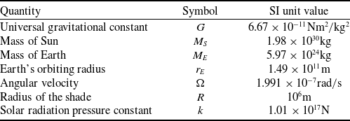
The system of governing equations given by Equation (7) and Equation (13) with forces and torques as described by Equations (32)–(36) is considered. This is by definition a linear system since linearisation was employed during the derivation of Equations (32)–(36). The parameter values used are as given in Table 1.
Parameters and values used in the model

Table 1. Long description
A table titled ‘Parameters and values used in the model’ contains seven rows and three columns. The columns are labeled ‘Quantity’, ‘Symbol’, and ‘SI unit value’. The table lists various astronomical and physical parameters along with their symbols and SI unit values. The rows are as follows: Row 1: Quantity, Universal gravitational constant; Symbol, G; SI unit value, 6.67 times 10 to the power of negative 11 newton meter squared per kilogram squared. Row 2: Quantity, Mass of Sun; Symbol, M subscript S; SI unit value, 1.98 times 10 to the power of 30 kilograms. Row 3: Quantity, Mass of Earth; Symbol, M subscript E; SI unit value, 5.97 times 10 to the power of 24 kilograms. Row 4: Quantity, Earth’s orbiting radius; Symbol, r subscript E; SI unit value, 1.49 times 10 to the power of 11 meters. Row 5: Quantity, Angular velocity; Symbol, omega; SI unit value, 1.991 times 10 to the power of negative 7 radians per second. Row 6: Quantity, Radius of the shade; Symbol, R; SI unit value, 10 to the power of 6 meters. Row 7: Quantity, Solar radiation pressure constant; Symbol, k; SI unit value, 1.01 times 10 to the power of 7 newtons.
The equilibrium position
 ${x_0}$
is found by equating to zero the terms not involving perturbations in Equation (32). In the absence of radiation pressure,
 ${x_0}$
reduces to the Lagrange point
 ${L_1}$
for a shade. When the radiation pressure is included, the equilibrium is shifted closer to the Sun. The eigenvalues associated with the equilibrium point are examined to determine which translational motions and which rotational motions are stable or unstable.
The two important parameters used to describe the shade are
 $\sigma $
and
 $\alpha $
. A
 $\sigma $
value of
 $765{\,\textrm{kg}}/{\textrm{k}}{{\textrm{m}}^2}$
results in a radiation pressure that can generate a force to balance the force due to Sun’s gravity for normal incidence. A sheet of paper typically weighs 50+ tons per
 ${\textrm{k}}{{\textrm{m}}^2}$
, so this density is two orders of magnitude lighter than paper. For
 $\alpha $
, a value of 0.001 means that the 1000 km radius shade has an axial extent of 1000 km.
With
 $\alpha = 0$
, two stable (centre, purely imaginary eigenvalue pair) and three unstable (saddle, positive and negative real eigenvalue pairs) modes are seen for all values of
 $\sigma $
. The two stable modes correspond to translational
 $y$
- and
 $z$
-displacements, while the unstable modes correspond to translational
 $x$
-displacement as well as rotational motions. For a given
 $\sigma $
, when
 $\alpha $
is increased, a change in stability of the rotational modes is observed as
 $\alpha $
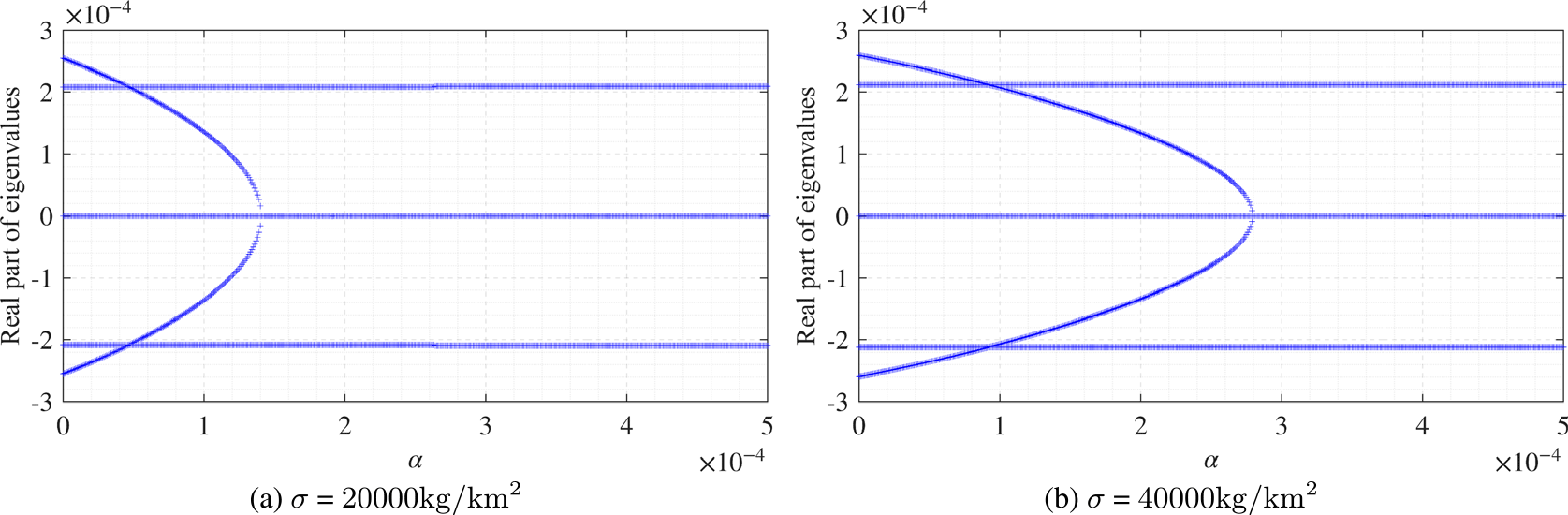
is increased beyond a cutoff. This is shown in Fig. 4, where after fixing the value of
 $\sigma $
at
 $20,000{\,\textrm{kg}}/{\textrm{k}}{{\textrm{m}}^2}$
and
 $40,000\frac{{{\textrm{kg}}}}{{{\textrm{k}}{{\textrm{m}}^2}}},$
respectively, in Fig. 4a and b,
 $\alpha $
is varied from 0 to 0.0005, and the real parts of the eigenvalues associated with a system equilibrium point are plotted. Since the eigenvalues arise in pairs with the same real parts, in Fig. 4a and b, there are only 5 loci for the loci plotted for the real parts of the 10 eigenvalues in each of the plots.
Real parts of the eigenvalues as the curvature parameter
 $\alpha $
is varied. There are 10 eigenvalues but there are only 5 loci, as more than 1 eigenvalue has the same real part. Simulation results for two different values of
 $\sigma $
have been shown.

The cases depicted in Fig. 4 are based on simulations involving paraboloid shades with uniform mass distribution. For all
 $\alpha $
values, a pair of real eigenvalues having the values
 $\pm 2.1 \times {10^4}$
is noted. This corresponds to the saddle point associated with the
 $x$
-displacement. The fixed points associated with the
 $y$
- and
 $z$
-displacements are centres and the corresponding eigenvalues are purely imaginary eigenvalues, with a zero real part, as shown in the diagram. In the case of
 $\sigma $
=
 $20,000{\,\textrm{kg}}/{\textrm{k}}{{\textrm{m}}^2}$
in Fig. 4a, for
 $\alpha $
values below
 $1.4 \times {10^{ - 4}}$
, a second pair of positive and negative real eigenvalues is observed to emerge. This pair, which actually occurs twice, corresponds to the two rotational modes. As
 $\alpha $
is increased from zero, the loci of the positive and negative eigenvalues are found to approach each other until they turn into a purely imaginary pair at
 $\alpha = 0.00014$
and remain so for higher values of
 $\alpha $
. A very similar trend is observed for
 $\sigma $
=
 $40,000{\,\textrm{kg}}/{\textrm{k}}{{\textrm{m}}^2}$
depicted in Fig. 4b, with the difference being that the cutoff value of
 $\alpha $
is higher (
 $\alpha = 2.8 \times {10^{ - 4}}$
) for stabilisation of the rotational modes.
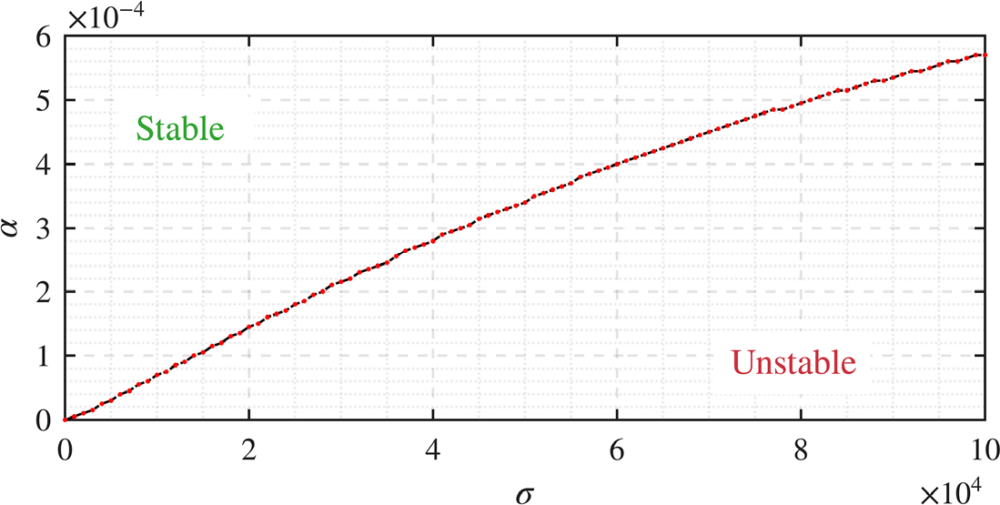
In Fig. 5, the cutoff value of
 $\alpha $
at which the rotational modes become stable is shown for different values of
 $\sigma $
. It can be seen that heavier shades need greater curvature to stabilise the rotational modes. This makes sense since gravity has a destabilising effect on these modes while radiation pressure has a stabilising one.
Transition curve in the
 $\sigma $
–
 $\alpha $
plane.

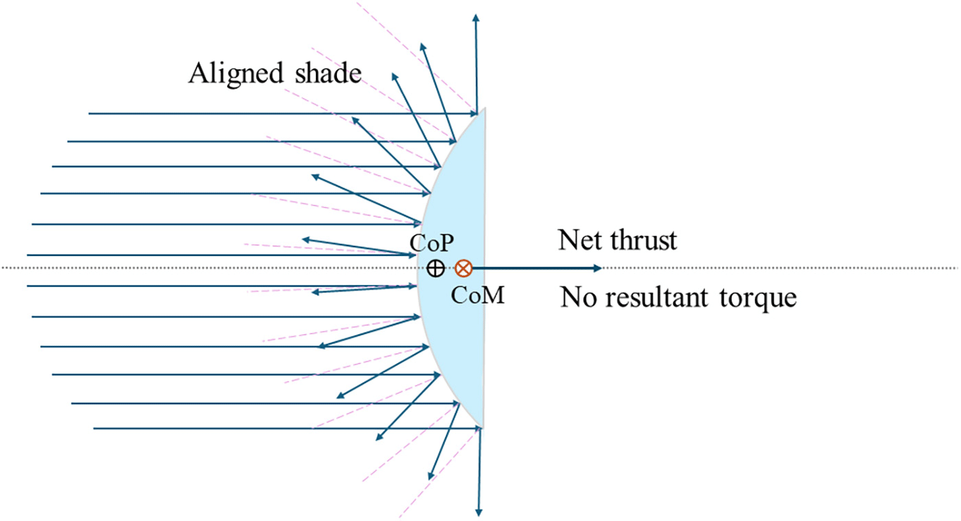
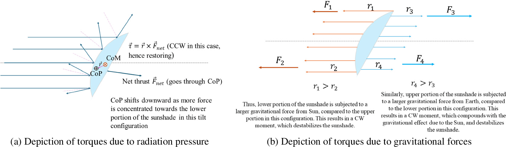
A set of illustrations is provided in Figs 6 and 7a and b to further elucidate the effects of radiation pressure and gravity with regard to stabilisation of rotational modes. The centre of pressure is computed by using the formula
 $\,{\vec {\!r}_{COP}} = {{\smallint \,\vec {\!r}d{F_{rp}}} \over {\smallint d{F_{rp}}}}$
, where
 $\,{\vec {\!r}_{COP}}$
is the centre of radiation pressure on the paraboloid shade,
 $d{F_{rp}}$
is the differential force due to radiation pressure at at a position
 $\vec r$
on the shade. The net resultant radiation force will pass through the centre of pressure located at
 $\,{\vec {\!r}_{COP}}$
.
An aligned configuration of the paraboloid shade, for depiction of the locations of the CoP and the CoM and the torque due to the radiation pressure.

A tilted configuration of the paraboloid shade, for depiction of the effects of gravitational forces from the Sun and the Earth on the shade and the resulting destabilising torque on the paraboloid shade.

As illustrated in Fig. 6, in an aligned configuration of a perfectly symmetric shade, the net resultant force is directed along the Sun-Earth axis and the
 $\,{\vec {\!r}_{COP}}$
and
 $\,{\vec {\!r}_{COM}}$
lie on the same axis. Here,
 $\,{\vec {\!r}_{COM}}$
is the CoM of the shade. The result is a net zero torque. In this configuration, the gravitational force due to the Sun and the Earth also does not result in a non-zero torque.
As illustrated in Fig. 7a, in a tilted configuration, the lower portion of the shade is subjected to higher radiation pressure compared to the upper portion of the shade owing to the closer orientation of the outward normal with the incident photon direction. The result is the movement of the centre of pressure (CoP) towards the lower portion of the shade. Given the net thrust
 $\,{\vec {\!F}_{rp,net}}$
passes through this location, the result is a counter-clockwise (CCW) torque about the CoM, which remains fixed. In this case, this is a restoring torque which provides stabilisation. A similar mechanism can be observed if the shade is tilted the other way, with the result being a clockwise (CW) restoring torque due to the radiation pressure force.
The effects of gravitational forces on the rotational mode stabilisation are illustrated through Fig. 7b. The gravitational forces comprise those due to the Sun’s gravity and the Earth’s gravity. When the shade is tilted in the configuration shown in Fig. 7b, the upper portions and the lower portions of the shade are at different distances from the Earth and the Sun, resulting in different gravitational forces, with the result being a torque in the CW direction for both the Sun’s and the Earth’s gravitational forces. This results in destabilisation of the shade.
4.0 Stabilisation considerations
Although a single degree of freedom control scheme is sufficient to stabilise the shade in theory, such a solution will not be robust in practice. Hence, an architecture is proposed to enable stabilisation of all possible modes of the shade. For this, it is sufficient for the shade to be able to generate a force in an arbitrary direction and a torque about an arbitrary axis.
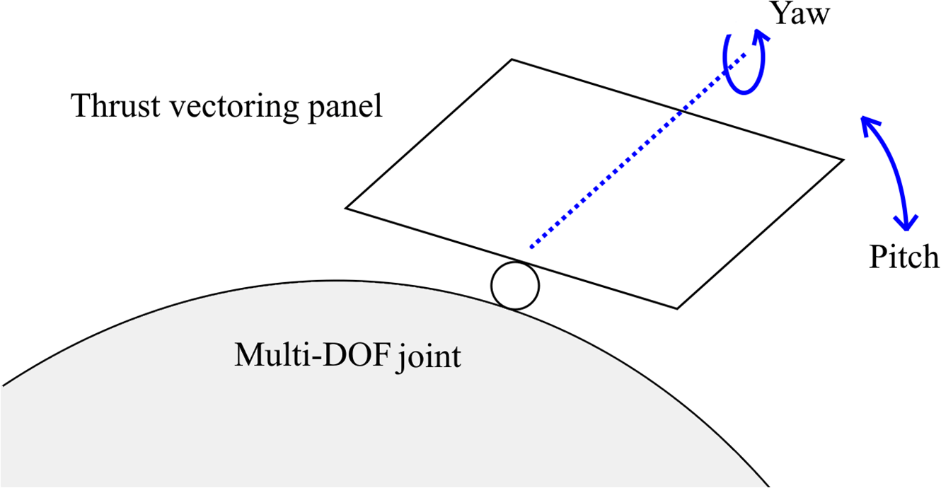
The proposed architecture consists of an array of movable panels all along the periphery of the shade together with a retractable panel at the centre. The peripheral panels are pivoted to the shade at one point so that the associated normal vectors can be oriented at any desired angle in space with respect to the symmetry axis of the shade. Practically, this means that two rotational degrees of freedom must be provided per panel. The configuration is shown in Fig. 8. By changing the configuration of the panel, one can vary the amount and direction of the SRP acting on the panel, thus adjusting the resultant force acting on the whole shade. The central panel can be designed to retract telescopically into itself; that is, overlap with other parts of the shade will be created so that this centre panel is no longer subject to SRP. The control is thus based on changing the shape of the shade. This concept is akin to shape change-based control concepts that have been studied by one of the authors in the context of control of ship crane load oscillations [Reference Kaipa and Balachandran25, Reference Li and Balachandran26]. A possible central panel retraction mechanism leading to the shade’s shape change is illustrated in Fig. 9. As illustrated in this figure, the panels occupying the central area of the shade are retracted behind the shade row-wise. This retraction is alternated between a row towards the top of the area and another towards the bottom. To fill the gap left by the retracted panels, the rows to the top/bottom cascade downwards/upwards to fill the gap. The panel sizes have been exaggerated in the schematic.
Schematic representation of a variable-geometry panel at the periphery of the shade.

Schematic representation of a possible mechanism for the retraction of the central panel for the proposed control architecture.

With the shade in the reference configuration, different panel adjustments can be used to realise different force outcomes as described below:
-
• Pitching up of two peripheral panels located 180 degrees apart would result in the generation of an
$x$
-direction force without moment. -
• Pitching up of two peripheral panels located at the ends of the
$y$
-axis and giving them opposite yaw angles will result in the retraction of the central panel. This will result in the generation of a
$z$
-direction force (the central panel retraction will compensate for the extra
$x$
-force arising from raising the peripheral panels). There is no moment generation. -
• A
$y$
-direction force may be generated exactly as described above, by activating panels at opposite ends of the
$z$
-axis. -
• Pitching up of the peripheral panel at the positive end of the
$y$
-axis and a suitable retraction of the central panel will result in the generation of a negative moment about the
$z$
-axis with no force. A positive moment is obtained if the panel at the negative end of the
$y$
-axis is activated. -
• A pure
$y$
-axis moment can be generated exactly as described above for a
$z$
-axis moment. -
• Pitching up of two panels at opposite ends of the shade with the same given nonzero yaw angle and appropriate retraction of the central panel will result in the generation of an
$x$
-axis moment.


Since
 $x$
axis is the major direction along which control is required, it is appropriate that the largest achievable forces are in that direction. The acceleration per unit control force is inversely proportional to the mass. When a control force
 ${F_{con}} = - {k_{con}}{\eta _x}$
is added to the force in Equation (32), it is expected that the
 $x$
-direction translation mode will also be stabilised. To examine this, the values
 $\sigma = 40,000{\,\textrm{kg}}/{\textrm{k}}{{\textrm{m}}^2}$
and
 $\alpha = 0.0004$
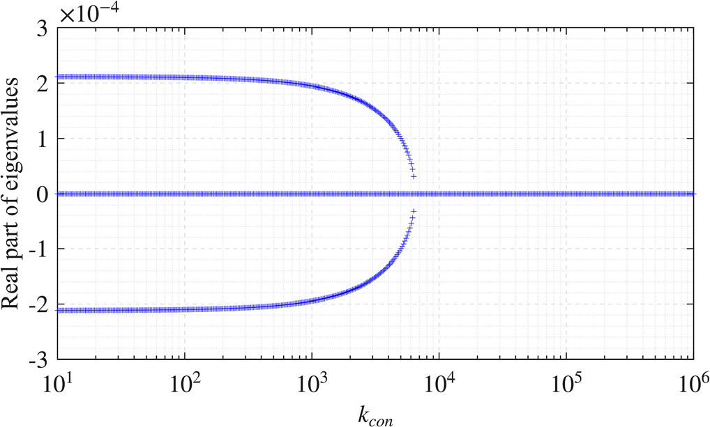
are considered. For this choice of parameter, all rotational modes are stable. Then, the control parameter
 ${k_{con}}$
is varied from 1 to
 ${10^{6}}{\textrm{N}}/{\textrm{km}}$
and the determined real parts of the eigenvalues are plotted in Fig. 10. As was observed with the rotational modes shown in Fig. 4 with respect to an increase in the
 $\alpha $
parameter, an identical behaviour is observed with the
 $x$
-translation mode as
 ${k_{con}}$
is increased, as shown in Fig. 10. Beyond a certain value of
 ${k_{con}}$
, there are no eigenvalues with non-zero real parts.
Plots of the real parts of the eigenvalues as
 ${k_{con}}$
is varied from a small value to a large value. It is noted that the
 $x$
-axis in this plot is on a logarithmic scale.

To numerically demonstrate control of the shade for motions along the
 $x$
axis, a simplified problem is considered. The simplification is necessary because the equations of motion used heretofore were obtained by linearisation about the apex of the shade. Next, the full nonlinear problem is considered with neglect of the rotational motions. The shade is treated as a disk that is always facing the Sun. Also, a two-dimensional motion (
 $x$
and
 $y$
only) is considered. The control strategy consists of varying the effective area
 $A$
of the shade exposed to the Sun. Let
 $A$
have the steady value such that the equilibrium radiation pressure is
 $k{A^{\rm{*}}} = 0.3G{M_S}$
, plus a perturbation
 ${\rm{\Delta }}A\left( t \right)$
which is used for control implementation. The equilibrium position is located at
 ${x^{\rm{*}}} = 1.326 \times {10^{11}}{\textrm{m}}$
. The specific relation chosen here is
 ${\rm{\Delta }}A = {10^{12}}\left( {x - {x^{\rm{*}}}} \right)/k$
. This corresponds to a stiffness
 ${k_{con}}$
exceeding
 $2 \times {10^6}{\textrm{N}}/{\textrm{km}}$
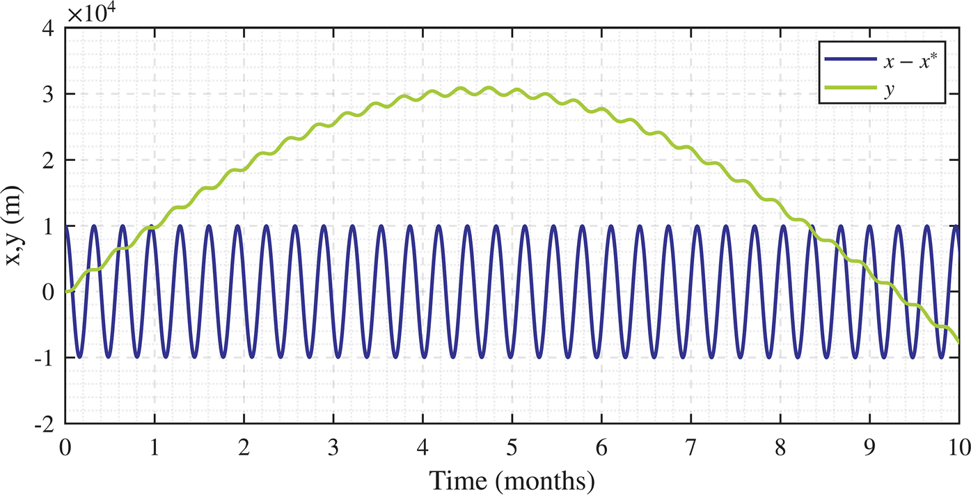
. For this control law, in Fig. 11, the variations in the
 $x$
direction and
 $y$
direction displacements of the shade over a nearly yearlong period are shown.
Plots of time traces of translational motions to illustrate stabilisation of a flat shade. The shade area is varied in proportion to the
 $x$
displacement.

Recalling that for the flat shade in the plane,
 $x$
direction displacements are unstable and
 $y$
direction displacements are stable, it is seen that control of the unstable translation mode alone is sufficient to stabilise the shade completely. This implies that for the paraboloid shade where five out of the six modes are inherently stable, control of the remaining mode will be sufficient to stabilise the shade. Nevertheless, the extensible solar panels enable control of all modes, for enhanced performance and stability.
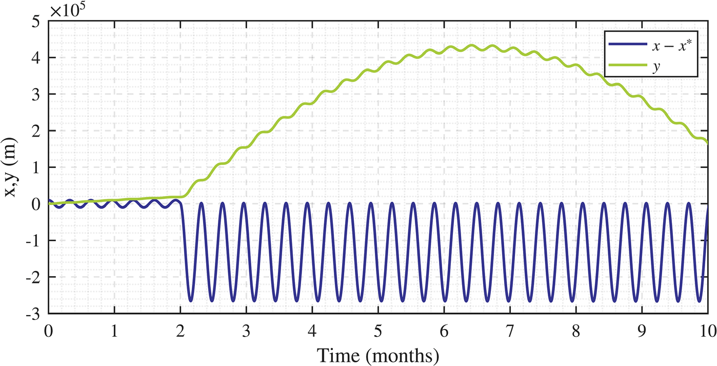
SRP is also subjected to temporal fluctuations as a result of the 11-year solar cycle and events like sunspots and solar storms. These variations are usually small, of the order of 0.1 percent [Reference Frohlich27–Reference Niccolai, Anderlini, Mengali and Quarta29]. A change in the radiation pressure, if not compensated by a change in effective area, can result in a significant shift of the equilibrium position of the shade, and hence give rise to large-amplitude oscillations between the old and new equilibrium positions. In Fig. 12, the situation of Fig. 11 is re-examined with
 $k{A^{\rm{*}}}$
being reduced by 0.3 percent after two months. The oscillation amplitude is seen to increase immediately. Although the amplitude and rapidity of the fluctuation in this schematic are significantly greater than what are observed in reality, for a precise control scheme, one will need to compensate for these fluctuations. Whenever such a motion is detected, the SRP will have to be measured, and the baseline area of the shade will have to be adjusted to keep the equilibrium in the same position.
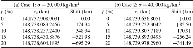
Equilibrium position shift due to reflectivity loss

Table 2. Long description
A table comparing equilibrium position shifts due to reflectivity loss in two cases. The table has two panels, each representing a different case. Panel A shows data for Case 1 with a reflectivity loss of 20,000 kilograms per square kilometer, and Panel B shows data for Case 2 with a reflectivity loss of 40,000 kilograms per square kilometer. Each panel contains four columns: f (percent), x0 (kilometers), and Shift (kilometers). The table has five rows, each representing different percentages of reflectivity loss (0 percent, 5 percent, 10 percent, 15 percent, and 20 percent). Panel A: Row 1: f, 0 percent; x0, 14,8737,908.9031 kilometers; Shift, 0 kilometers. Row 2: f, 5 percent; x0, 148,738,083.2456 kilometers; Shift, 174.34 kilometers. Row 3: f, 10 percent; x0, 148,738,257.2400 kilometers; Shift, 348.34 kilometers. Row 4: f, 15 percent; x0, 148,738,430.8876 kilometers; Shift, 521.98 kilometers. Row 5: f, 20 percent; x0, 148,738,604.1895 kilometers; Shift, 695.29 kilometers. Panel B: Row 1: f, 0 percent; x0, 148,739,636.8051 kilometers; Shift, 0 kilometers. Row 2: f, 5 percent; x0, 148,739,722.3042 kilometers; Shift, 85.50 kilometers. Row 3: f, 10 percent; x0, 148,739,807.7189 kilometers; Shift, 170.91 kilometers. Row 4: f, 15 percent; x0, 148,739,893.0495 kilometers; Shift, 256.24 kilometers. Row 5: f, 20 percent; x0, 148,739,978.2960 kilometers; Shift, 341.49 kilometers.
Plots of time traces of translational motions to depict stabilisation of a flat shade. The shade’s area is varied in proportion to the
 $x$
displacement. After two months, the value of radiation pressure suddenly drops by 0.3 percent, causing a substantial increase in amplitude of the oscillations.

A factor complicating the control of the shade will be the delay in the loop arising from the distance between the Earth-based control station and the shade itself. It takes light approximately 5 s to travel from Earth to the
 ${L_1}$
point. This would mean a minimum 10 s delay is bound to enter the control loop. A delay added to a neutrally stable system (harmonic oscillator) can destabilise this system. This can be countered by activating the panels to simulate damping of all modes of motion. A control algorithm based on the estimated position after the delay interval can also be incorporated.
In the next few subsections, the authors discuss a few stabilisation aspects that will need to be considered for detailed analyses in the future to be utilised for the practical implementation of the discussed shade concept.
4.1 Material reflectivity degradation
A set of investigations has been carried out to understand the effect of degradation of material reflectivity on the stability analysis of the shade. The results obtained are presented here.
The radiation pressure constant
 $k$
depends on the surface reflectivity of the shade, which is expected to change over the operational lifetime of the shade owing to different factors. A few simulations using optimal and slightly diminished values of
 $k$
for two different values of
 $\sigma $
were carried out to investigate the effect of material reflectivity loss on the equilibrium position
 ${x_0}$
. For these simulations, the radiation pressure constant
 $k$
was computed by using
 $\left( {1 - f} \right){k_0}$
, where
 ${k_0}$
is the nominal radiation pressure coefficient and
 $f$
is the fractional reflectivity loss. The results obtained for the two cases
 $\sigma = 20,000{\,\textrm{kg}}/{\textrm{k}}{{\textrm{m}}^2}$
,
 $\alpha = 0.0005{\textrm{k}}{{\textrm{m}}^{ - 1}}$
and
 $\sigma = 40,000{\,\textrm{kg}}/{\textrm{k}}{{\textrm{m}}^2}$
,
 $\alpha = 0.0005{\textrm{k}}{{\textrm{m}}^{ - 1}}$
(both stable regions) are summarised in Table 2.
From the results presented in Table 2, it can be inferred that due to the degradation of reflectivity, the net effect of the different forces results in a net sunward force at the nominal equilibrium position due to the reduced radiation pressure. To compensate for this force imbalance and realise a state of equilibrium, the position of the paraboloid shade needs to be shifted towards the Earth as outlined in Table 2. The equilibrium position shifts linearly for the reflectivity loss, with a
 $35{\,\textrm{km}}$
shift for
 $1{{\% }}$
reflectivity loss for
 $\sigma = 20,000{\,\textrm{kg}}/{\textrm{k}}{{\textrm{m}}^2}$
and around
 $17{\,\textrm{km}}$
shift for
 $\sigma = 40,000{\,\textrm{kg}}/{\textrm{k}}{{\textrm{m}}^2}$
.
The control architecture to compensate for this equilibrium shift involves the coordinated use of the peripheral panels to generate decoupled forces and moments as outlined in Section 4. The relevant control mode for this is the generation of a pure x-direction force that can be achieved by pitching up of two peripheral panels located
 ${180^ \circ }$
apart. Partially tilted peripheral panels in the reference configuration can help in adjusting the radiation pressure force in either direction in such cases. They can be rotated towards the Sun-facing orientation, increasing the effective radiation pressure contribution and restoring the outward force. Given the peripheral panels have an area of
 ${A_p}$
, the total shade area is
 $A$
, and considering the case where the nominal tilted configuration makes an angle
 $\beta $
with the Sun-Earth line, the maximum additional force which can be generated is
 $\frac{{{A_p}}}{A}\left( {1 - {\textrm{co}}{{\textrm{s}}^2}\beta } \right){F_{{\textrm{rad}}}}$
. Thus, to compensate for the reflectivity loss
 $f$
, we should have to satisfy
 $\frac{{{A_p}}}{A}\left( {1 - {\textrm{co}}{{\textrm{s}}^2}\beta } \right) \ge f$
.
4.2 Mass budget of the control system
Another stability constraint required to be considered is the mass budget of the control system. The proposed control architecture consists of actuators and hinges at the periphery, which together introduce additional mass towards the periphery. As a result, the CoM
 ${o_B}$
is shifted axially towards the rim of the paraboloid shade.
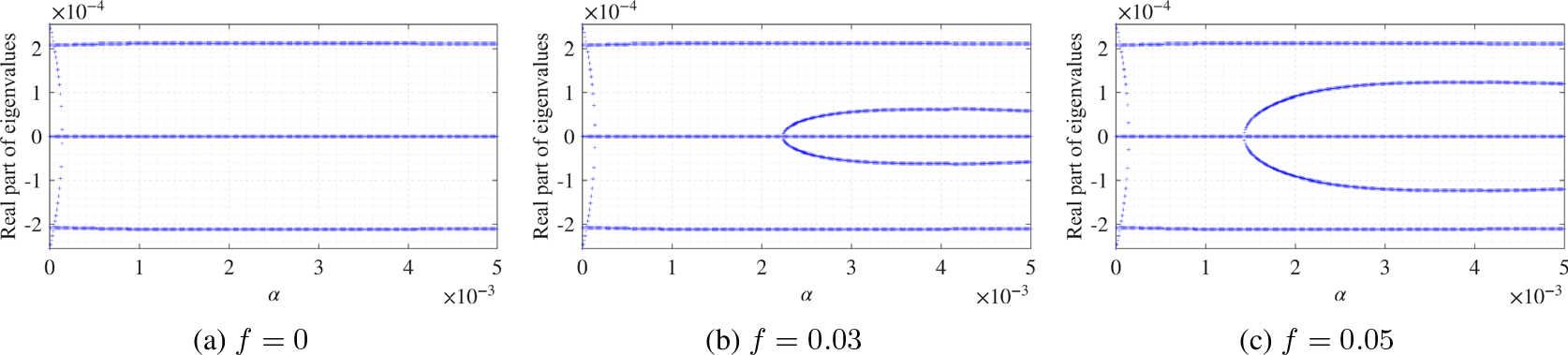
Real parts of eigenvalues for investigation of peripheral mass distribution on paraboloid shade stability, as the curvature parameter
 $\alpha $
is varied. Results of simulations for three different values of the rim mass enhancement factor
 $f$
have been shown for areal density
 $\sigma = 20,000{\,\textrm{kg}}/{\textrm{k}}{{\textrm{m}}^2}$
.

To investigate the effect of
 ${o_B}$
shift on the shade stability, the mass distribution over the paraboloid shade is made non-uniform through the use of two parameters, namely
 ${r_{rim}}$
and
 $f$
. Here,
 $f$
is the rim mass enhancement factor and
 ${r_{rim}}$
is the rim location. The CoM
 ${o_B}$
is then calculated using the formula in Equation (37).
 \begin{align}o_{B}=\frac{\displaystyle\int_{r\leq r_{\mathrm{rim}}}\alpha\left(q^{2}+d^{2}\right)w_{0}\,\mathrm{d}q\,\mathrm{d}d+\int_{r_{\mathrm{rim}}\leq r\leq R}(1+f)\alpha\left(q^{2}+d^{2}\right)w_{0}\,\mathrm{d}q\,\mathrm{d}d}{\displaystyle\int_{r\leq r_{\mathrm{rim}}}w_{0}\,\mathrm{d}q\,\mathrm{d}d+\int_{r_{\mathrm{rim}}\leq r\leq R}(1+f)w_{0}\,\mathrm{d}q\,\mathrm{d}d}\end{align}
This effectively means that the annular area marked by
 ${r_{rim}}$
has a larger areal density
 $\left( {1 + f} \right)\sigma $
, which results in the uneven mass distribution.
Simulations have been carried out for different values of
 ${r_{rim}}$
and
 $f$
for shades with different areal density
 $\sigma $
. The numerical studies have revealed a few important things as discussed below.
-
• Though the absolute
${o_B}$
values increased rapidly with
$\alpha $
(increasing from
${o_B} \approx 264{\,\textrm{km}}$
at
$\alpha = 0.0005$
to
${o_B} \approx 5990{\,\textrm{km}}$
at
$\alpha = 0.01$
), the fractional impact of rim mass enhancement factor
$f = 0.05$
from a uniform to non-uniform mass distribution on
${o_B}$
shift is around
$\approx 0.184{{\% }}$
over the range of
$\alpha $
. For
$f = 0.03$
, the fractional
${o_B}$
shift comes down to
$\approx 0.12{{\% }}$
. -
• The rotational stability structure of the shade has been found to be very sensitive to the shift in the
${o_B}$
position (mass distribution). The evolution of eigenvalues for
$\sigma = 20,000{\,\textrm{kg}}/{\textrm{k}}{{\textrm{m}}^2}$
for a range of rim mass enhancement values
$f$
is depicted in Fig. 13. In all these cases, the enhanced mass is concentrated in the outermost
$2{{\% }}$
of the shade. In the uniform-mass case
$\left(\, {f = 0} \right)$
, the rotational mode is stable for all
$\alpha $
above
$1.4 \times {10^{ - 4}}$
. For nonzero
$f$
, an instability appears within the otherwise-stable region, as can be observed in Fig 13b and c. A pair of eigenvalues has non-zero real parts over a finite range of
$\alpha $
, producing an ‘unstable bubble’ in the stability map. -
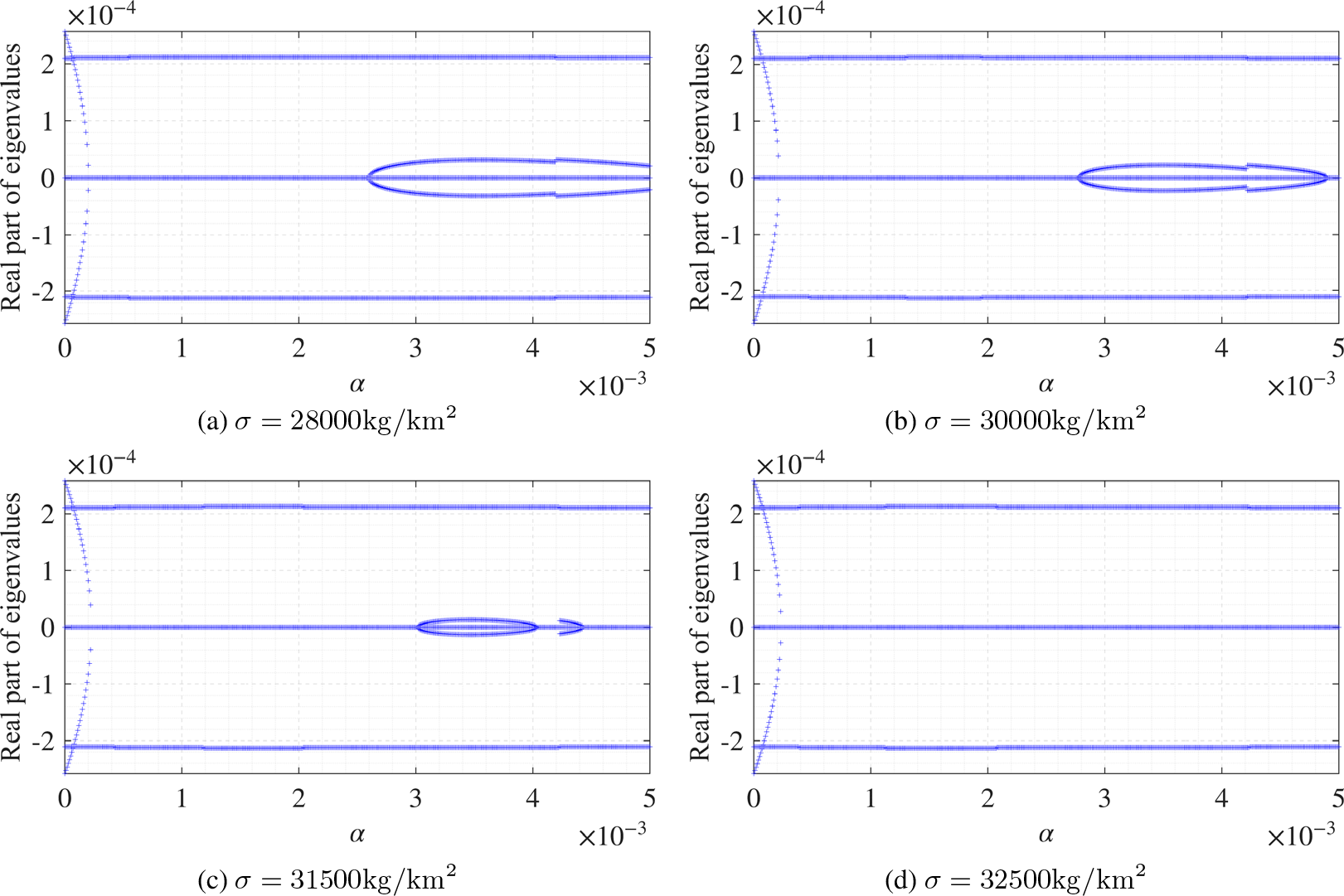
• The influence of the areal density on the stability regime of the paraboloid shade for non-uniform mass distribution was also investigated through another set of simulations. A representative figure depicting the stability behaviour for four areal density values for
$f = 0.03$
is illustrated in Fig. 14. It can be observed from the plots in Fig. 14 that the region of stability for rotational modes expands with an increase in areal density
$\sigma $
. The instability bubble observed for
$\sigma = 28,000{\,\textrm{kg}}/{\textrm{k}}{{\textrm{m}}^2}$
slowly diminishes and disappears at
$\sigma = 32,500{\,\textrm{kg}}/{\textrm{k}}{{\textrm{m}}^2}$
.


Real parts of eigenvalues for investigation of peripheral mass distribution on paraboloid shade stability, as the curvature parameter
 $\alpha $
is varied. Results of simulations for four different values of the areal density
 $\sigma $
have been shown for the rim mass enhancement factor
 $f = 0.03$
.

It can be inferred from the above set of simulation results that the mass distribution of the control hardware remains a critical design parameter for the architecture, and the control system mass budget must be specified exactly as part of any operational implementation. Compensation strategies can include optimal choice of
 $\alpha $
and
 $\sigma $
based on stability maps as well as use of counter-masses on the anti-Sun side of the shade close to the apex. This can be used for restoring the wider stability range of the uniform-density case.
4.3 Non-linear recovery for larger angular perturbations
As mentioned in Section 2.2, the stability analysis presented in this study is based on a rigid body model of the shade. Second, only small perturbations of the different Euler angles were assumed in Section 2.2, which was then followed by the derivation of the different force and torque equations. This has been carried out through a linearisation of the equations of motion about the equilibrium configuration, which is valid in the limit of small angular perturbations. However, to verify that the linear stability conclusions remain quantitatively valid for moderate perturbations of practical interest, a representative single degree-of-freedom rotational simulation was conducted and is presented here.
The investigated case is for the parameters
 $\sigma = 40,000{\,\textrm{kg}}/{\textrm{k}}{{\textrm{m}}^2}$
and
 $\alpha = 5 \times {10^{ - 4}}{\textrm{k}}{{\textrm{m}}^{ - 1}}$
. As depicted in Fig. 4b, stabilised rotational modes occur for this choice. The linearised rotational dynamics for this state can be said to be governed by an oscillator with a natural frequency of
 $\omega = 1.88 \times {10^{ - 4}}$
rad/s, which is the imaginary part of the corresponding eigenvalue. Physics wise, this corresponds to the rotational mode near the equilibrium, which can be modeled as follows:
 \begin{align}{\ddot{\theta}} + \omega^{2}\theta = 0\end{align}
Here,
 $\theta $
denotes the libration angle of the shade’s symmetry axis relative to the equilibrium (Sun-pointing) orientation, considered for a single transverse rotation axis. From the rotational symmetry, the single degree-of-freedom treatment considered for the simulations here is representative for both the pitch and roll modes.
A representative nonlinear extension of Equation (38) can be obtained by replacing the linear restoring torque with the form
 ${\omega ^2}{\textrm{sin}}\theta {\textrm{cos}}\theta $
, which reduces to the linear case at small angles. While the considered single degree-of-freedom model does not capture the full coupling present in the multi degree-of-freedom model of the original system, this analysis serves as a representative test of whether the period of oscillation is significantly altered by the nonlinear
 ${\textrm{sin}}\theta {\textrm{cos}}\theta $
dependence of the restoring torque.
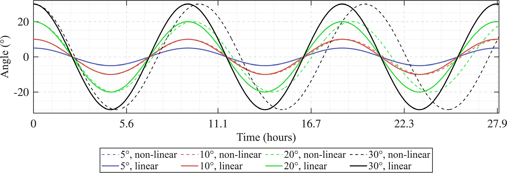
As depicted in Fig. 15, for initial perturbations of
 ${5^ \circ }$
and
 ${10^ \circ }$
, the nonlinear oscillation period departs from the linear prediction by
 $0.25{{\% }}$
and
 $0.85{{\% }},$
respectively. It is observed that the trajectory remains within
 ${0.17^ \circ }$
and
 ${1.32^ \circ }$
of the linear solution over multiple oscillation periods. However, the deviations between the linear solutions and the non-linear oscillations grow with amplitude. This becomes clear in the plots depicted in Fig. 15 beyond
 ${20^ \circ }$
. The results confirm that the linearised stability conclusions are quantitatively reliable throughout a moderate perturbation range till
 ${15^ \circ }$
. A complete nonlinear analysis with a multi degree-of-freedom model, including translation–rotation coupling and pitch and roll coupling, is identified as an important direction for future investigation.
Evolution of the recovery from different initial angular perturbations ranging from
 ${5^ \circ }$
to
 ${30^ \circ }$
. Dashed lines are used to depict the non-linear recovery trajectories and solid lines are used to depict the trajectories following the solution of the linearised eigenvalue problem.

5.0 Practical feasibility and limitations of the study
The work presented here is intended to serve as an initial foundation for the development of a paraboloid shade. To proceed further, one needs to address the associated limitations in terms of material properties, structural dynamics and other practical considerations for the construction of the shade. One important aspect is the construction of the paraboloid shade and the materials that can be utilised for this purpose. The value of
 $\sigma = 765{\,\textrm{kg}}/{\textrm{k}}{{\textrm{m}}^2}$
mentioned in Section 3.2 has been obtained through balancing of solar gravity and SRP forces, assuming perfect absorption when the curvature factor
 $\alpha = 0$
. Current space-qualified materials include aluminised polymer films like Kapton [30], which has a bulk density of
 $1420{\,\textrm{kg}}/{{\textrm{m}}^3}$
. The required thickness to achieve the above-mentioned surface density will be 550 nm (0.55
 ${\rm{\mu }}$
m). In the James Webb Space Telescope (JWST), five layers of Kapton [31] have been used, with the Sun-facing layer having a thickness of 50
 ${\rm{\mu }}$
m and each subsequent layer having a 25
 ${\rm{\mu }}$
m thickness. The surface density of a 25
 ${\rm{\mu }}$
m-thick Kapton sheet is about 35
 ${\textrm{g}}/{{\textrm{m}}^2}$
. With less-thick Kapton sheets, one can achieve the suggested surface density; however, this might result in brittleness of the structure. Aerographite is one of the lightest structural materials ever created, having a bulk density of
 $0.18{\rm{\;g}}/{{\textrm{m}}^3}$
[Reference Heller, Anglada-Escud´e, Hippke and Kervella32]. However, they can be fragile and have not been produced in large sheets. Beyond density, the shade material must also be able to survive UV and particle radiation over decades alongside thermal extremes. With an increase in curvature parameter
 $\alpha $
, the areal density required for stabilisation of the rotational modes will increase, which will allow for further options in materials that can be utilised.
In addition to this, the size of the paraboloid shade should also be carefully considered. That is independent of the material chosen for the construction. For a shade radius =
 $1000$
 ${\textrm{km}}$
, the total mass of the shade would be around 2.4 million tonnes when
 ${\rm{\alpha }} = 0$
, which is an exceptional logistical challenge. To partially address this challenge, a paraboloid of smaller radius can be explored.
The portion of the Sun’s disc blocked by a shade of radius r at a distance of d from the Earth can be approximated by:
 \begin{align}f= \frac{{{\textrm{solid angle of Sun blocked by shade}}}}{{{\textrm{solid angle of Sun}}}},\end{align}
where the solid angle
 ${\rm{\Omega }} = \pi {\theta ^2}$
and
 $\theta $
is the angular radius. As seen from a point on Earth, the angular radius subtended by the shade is
 \begin{align}{\theta _{{\textrm{shade}},{\textrm{Earth}}}} = \frac{r}{d} = \frac{{1000}}{{1,500,000}} = 6.67 \times {10^{ - 4}}{\textrm{rad}}.\end{align}
The angular radius subtended by the Sun is
 \begin{align}{\theta _{{\textrm{Sun}}}} = \frac{{{R_{{\textrm{Sun}}}}}}{{{d_{{\textrm{Sun}}}}}} = \frac{{696,000}}{{149,600,000}} = 4.65 \times {10^{ - 3}}{\textrm{rad}}.\end{align}
After using these values, the result is
 \begin{align}f = \frac{{\pi \theta _{{\textrm{shade}},{\textrm{Earth}}}^2}}{{\pi \theta _{{\textrm{Sun}}}^2}} = {\left( {\frac{{{\theta _{{\textrm{shade}},{\textrm{Earth}}}}}}{{{\theta _{{\textrm{Sun}}}}}}} \right)^2} = 2.05{{\% }}.\end{align}
For
 $r = 500$
km, this fraction reduces to
 $f = 0.51{{\% }}$
. Therefore, more than one such paraboloid Sun shade would be needed to achieve the same amount of blocking.
In sum, realisation of the prescribed density with sufficient tensile strength, radiation tolerance and operational lifetime over decadal timescales is a materials science challenge that has not been addressed in the existing literature and should be treated as a primary constraint in any follow-on systems study.
With regard to structural dynamics, in the present paraboloid shade analysis, as a first step, it has been assumed that the shade is a perfect rigid body with fixed moments of inertia and the curvature parameter
 $\alpha $
. This assumption is a significant idealisation for a structure of this scale. The following limitations need to be addressed for a practical realisation of the proposed concept:
-
• The stability scenarios established in this study depend on the curvature parameter
$\alpha $
. This parameter determines the location of the centre of SRP (CoP) relative to the CoM of the structure, and consequently, the SRP restoring torque coefficient. The stability boundaries depicted in Figs 4 and 13 are calculated based on a spatially constant value of
$\alpha $
, which may not hold due to the uneven distribution of the SRP on the structure. The SRP will decrease from the paraboloid apex towards the rim when
$\alpha \gt 0$
, and the non-uniform loading can cause the membrane to deform out of the normal paraboloid shape, which is referred to as billowing. This billowing can alter the SRP torque, and thus, the shade’s stability.


For axisymmetric billowing of a perfect paraboloid structure, the virtual focal point will be shifted along the Sun-Earth axis. This point moves closer to the surface when the shade curves more (increases
 $\alpha $
) and moves farther away when the shade flattens (decreases
 $\alpha $
). A single, well-defined focal point is preserved in this case. For non-axisymmetric billowing, the effective focal point becomes an extended region, as different parts of the shade deflect rays from different virtual locations. The CoP location will deviate from the location determined from the rigid body analysis, which can result in the generation of spurious torques and alter stability scenarios.
Wrinkling [Reference Huang, Zeng, Circi, Vulpetti and Qiao33] can result in localised inverted surface curvatures, which can lead to non-uniform force fields resulting in deviation from the SRP torque calculated based on the rigid-body assumption, and subsequently, stability regions.
-
• Shape oscillations can have a dynamic effect as well, wherein the structural vibration can result in time-varying
$\alpha $
. In turn, this can result in the introduction of a parametric excitation [Reference Chen, Shi, Dowell and Pei34] to the system and result in oscillations. The parametric instability mechanism is not present in the current rigid-body modeling and needs to be investigated in future studies. -
• Solar radiation simultaneously results in mechanical pressure as well as a thermal load [Reference Boni, Quarta and Mengali35] on the sunward face of the shade. The resulting temperature gradient across the small membrane thickness can induce a bending moment that can deform the membrane. Such deformations can alter
$\alpha $
in a non-uniform, spatial manner, which depends on the thermal properties of the material and temperature distribution. These aspects have not been included in the present model.


To summarise, in the rigid body model presented in this study, a constant
 $\alpha $
is assumed for the stability analysis. However, as discussed above,
 $\alpha $
can get spatially non-uniform due to a number of reasons, and a shade designed to operate at a particular
 $\alpha $
range can become unstable. As elucidated in Section 4, changes in alpha by
 $10{{\% }}$
can result in unstable rotational motion for the shade, and this warrants a complete stability assessment for which the membrane deformation and attitude motion will need to be determined simultaneously, with the actual equilibrium shape determined by the combined SRP, gravity-gradient, centrifugal and thermal loading in the reference configuration rather than by the nominal undeformed paraboloid.
6.0 Closure
In this article, the dynamics and stabilisation of a paraboloid shade at or near the Lagrange point
 ${L_1}$
point has been considered. It has been shown that for certain choices of the material density and curvature of the shade, all translation and rotation modes are stable other than the translational displacement along the Sun-Earth axis. A control strategy based on variable-orientation solar panels has been proposed to stabilise the
 $x$
-direction translation as well as add additional stability to the other modes if the need arises. In future work, different stabilisation considerations and aspects discussed in Sections 4 and 5 will need to be examined. Particularly, flexible body effects like time-varying moments of inertia, billowing and wrinkling, as well as thermal instabilities, will need to be integrated for a better practical realisation of the proposed shade at operationally relevant scales. Furthermore, the mass budgeting system for effective control of the shade and implications of the delay in the control loop due to the distance of the shade from Earth will need to be investigated.
To close, it is remarked that space-based solar shading is presented as a temporary solution to mitigate the effects of climatic warming, and not as an alternative to pursue efforts on Earth to combat this climate change.
Acknowledgement
The third author acknowledges the support of the Minta Martin Professorship for this study.
Author contributions
The author contributions are as follows: BS: Methodology, Software, Validation, Formal analysis, Investigation, Data curation, Writing – original draft. SC: Software, Investigation, Analysis, Writing- Editing. BB: Conceptualisation, Methodology, Analysis, Writing – review and editing, Supervision, Funding acquisition.
Competing interest
The authors have no competing interests.
 α
 σ
 σ
 α

 kcon
 x
 x
 x
 α
 f
 σ=20,000kg/km2
 α
 σ
 f=0.03
 5∘
 30∘

 Open access

