1. Introduction
The large-scale flow in the atmosphere and the ocean appears to be approximately in geostrophic balance and thus divergence free (Gill Reference Gill1982). The scale separation between fast gravity waves and slowly evolving balanced flow supports this observation. In a celebrated article, Rossby (Reference Rossby1938) used the one-dimensional rotating shallow water equations (RSW hereafter) to illustrate the phenomenon of geostrophic adjustment, where an unbalanced initial state attains balance after a long time due to the radiation of waves away from the local region of excitation. This remarkable result was due to the fact that the linear potential vorticity (hereafter PV) is independent of the wave activity and does not evolve in inertial time. Thus, the state of the system after a long time can be obtained by equating the initial and final PV, and then inverting the PV to get the velocity and pressure (or height) field. This was followed by a series of works that addressed the problem in different contexts and greater detail (see Blumen (Reference Blumen1972) and references therein). The scale separation between fast waves and balanced flow was used by Charney (Reference Charney1948) and Obukhov (Reference Obukhov1949) independently to derive the quasi-geostrophic (QG) equation. The most remarkable feature of QG theory is that one can track the slow evolution of the balanced flow without having any information on the dynamics of fast waves in the system.
This was followed by the introduction of the idea of a slow manifold (Leith Reference Leith1980; Lorenz Reference Lorenz1980), whereby the evolution of the balanced flow is obtained by projecting the dynamics onto a subset of the whole space. The slow manifold – its existence and exact definition – has been debated since its introduction (Lorenz Reference Lorenz1986; Vautard & Legras Reference Vautard and Legras1986; Lorenz & Krishnamurty Reference Lorenz and Krishnamurty1987). A major challenge to its existence is the phenomenon of spontaneous generation, by which an initially balanced flow can develop wave activity in finite time. Although investigations in this direction seem to indicate the non-existence of the slow manifold in its strict sense as a manifold of zero thickness in state space, at present, conventional wisdom seems to have established that in the regime
 $Ro\sim Fr\ll 1$
, where
 $Ro$
(ratio of rotational time scales to advective time scales) and
 $Fr$
(ratio of flow velocity to wave speed) refer to the Rossby and Froude numbers respectively, often called the QG regime, the amplitude of the waves excited spontaneously is exponentially small (see Vanneste (Reference Vanneste2013) and references therein and Vanneste & Yavneh (Reference Vanneste and Yavneh2004) for a specific example).
The problem we address in this work is not the evolution of balanced initial data and subsequent spontaneous generation of waves, but rather the evolution of unbalanced initial data in RSW and the resulting interaction between the waves and the balanced flow, both being of comparable magnitude. In such a setting, for
 ${\it\epsilon}=Ro\sim Fr\ll 1$
, several works have used formal asymptotic methods to derive the QG equation in RSW more systematically and establish the absence of the fast motion affecting the balanced flow up to
 $O({\it\epsilon})$
. Majda & Embid (Reference Majda and Embid1998) in spectral space and Dewar & Killworth (Reference Dewar and Killworth1995) in physical space illustrated that the geostrophic field is unaffected by the waves for time scales
 $t\lesssim 1/({\it\epsilon}f)$
,
 $f$
being the inertial frequency. Further numerical simulations by Dewar & Killworth showed a lack of energy exchange between the waves and the geostrophic modes. From a turbulence perspective, Warn (Reference Warn1986) used statistical mechanics investigations on RSW to conclude that after a long time most of the energy ends up with the waves. Warn speculated about the possibility of energy exchange between waves and geostrophic modes in the long-time limit. In a low-order truncated forced-dissipative setting, the presence of gravity waves even after long times was pointed out by Warn & Menard (Reference Warn and Menard1986). Careful numerical experiments on RSW by Farge & Sadourny (Reference Farge and Sadourny1989), however, did not find any energy exchange between the waves and the balanced flow, although they found that the presence of inertio-gravitational energy in the system prevented the inverse energy cascade of the geostrophic flow. Farge & Sadourny did point out the possibility that artificial dissipation, used for numerical stability in their simulations, could have prevented the system from relaxing to statistical equilibrium. The inertio-gravity waves in RSW, due to their specific form of dispersion relation, do not allow triad interactions (Babin, Mahalov & Nicolaenko Reference Babin, Mahalov and Nicolaenko1997; Majda Reference Majda2002). Hence, there are no resonant wave triads although the geostrophic modes can catalyse interaction between wave modes. This was investigated in detail by Ward & Dewar (Reference Ward and Dewar2010), who showed that a coherent wave energy distribution can be scattered and inhomogenized by the geostrophic modes. Numerical simulations of reduced models and a full RSW system did not find any energy exchange between the waves and the balanced flow. In an unbounded domain with compactly supported unbalanced initial data, which is the classical setting for the geostrophic adjustment problem, the waves do not influence the balanced flow even with nonlinear interactions due to their rapid propagation away from the initial region. Reznik, Zeitlin & Ben Jelloul (Reference Reznik, Zeitlin and Ben Jelloul2001) (RZB hereafter) used multiple time scale asymptotics in such a setting to argue that the waves do not affect the balanced flow up to
 $t\sim 1/({\it\epsilon}^{2}f)$
in RSW. Reznik & Grimshaw (Reference Reznik and Grimshaw2002) further investigated the adjustment problem in the half-plane, i.e. in the presence of a boundary at
 $y=0$
, a setting that can support Kelvin waves. For different sets of initial conditions considered, except in the case of periodic initial data in
 $x$
where the Kelvin waves were seen to affect the evolution of balanced dynamics, geostrophic adjustment leading to the slow evolution of the balanced flow unaffected by the waves was observed in all other cases. In a barotropic rotating fluid, without making the classical traditional approximation, i.e. neglecting the projection of Coriolis force on the rotating plane and in the absence of hydrostatic balance, Reznik (Reference Reznik2014) showed that gyroscopic waves can affect the evolution of balanced dynamics in the long-time limit.
At present, conventional wisdom seems to be that in the regime
 $Ro\sim Fr\ll 1$
of RSW with unbalanced initial data that can excite inertio-gravity waves and balanced flow of equal magnitude, the geostrophically balanced flow evolves slowly, as described by the QG equation, unaffected by the waves, while the balanced flow can catalyse interactions between the fast waves. The possibility of fast waves influencing the balanced flow in this regime still remains an open question, in spite of the many advances that have been made in geophysical flows. The differences in the various types of models used (forced-dissipative, truncated-inviscid, etc.) in the numerical works previously described also lead to different answers. The only theoretical work that has investigated the state of unbalanced initial conditions for very long time scales (
 $t\sim 1/({\it\epsilon}^{2}f)$
) in this particular parameter regime of RSW with an eye on the possibility of inertio-gravity waves affecting balanced dynamics, to the best of the present author’s knowledge, is RZB, their set-up being an unbounded domain with compact initial data, leading to geostrophic adjustment. This sets the main motivation for the present theoretical work aimed at investigating the possibility of fast waves affecting the balanced flow by investigating the evolution of unbalanced initial data in RSW.
We use the method of multiscale asymptotics to investigate fast–slow interactions in RSW. The initial conditions are arbitrary or unbalanced with data that would project on fast modes and balanced flow, the fast part consisting of inertio-gravity waves and inertial oscillations. Periodic and unbounded domains are given particular attention in the analysis. The periodic domain is given special emphasis as in such a setting the waves do not radiate to infinity leaving behind the balanced flow. In real geophysical flows such as in the atmosphere or the ocean, waves and balanced flow interact continuously for very long times. A finite domain with periodic boundary conditions acts as the simplest test bed to study such long-time interactions between waves and balanced flow.
In § 2, we proceed systematically using asymptotics to derive a higher-order slow evolution equation in RSW that is valid for
 $t\lesssim 1/({\it\epsilon}^{2}f)$
, i.e. a time scale exceeding that of QG dynamics (which is
 $t\lesssim 1/({\it\epsilon}f)$
). This new slow equation, accurate up to
 $O({\it\epsilon}^{2})$
, is used to argue that waves can influence the slow dynamics. We then show that the slow energy equation is not closed, but can exchange energy with fast waves. Potential enstrophy, which is seen to be an exact invariant of this new slow equation, is also affected by the waves. In § 3, we set up the problem in a periodic domain and use resonant wave interaction theory to construct a simple reduced system that illustrates fast waves influencing balanced flow. In this special system, the waves act as catalysts, modifying energy exchange between geostrophic modes. Section 4 summarizes the findings of the present work.
2. General results
We will use the method of multiple time scale asymptotics (see, e.g., Ablowitz (Reference Ablowitz2011), Chap. 4 for the particular method that we employ) to investigate the interaction between fast modes and slow balanced flow in RSW. Although the analysis in this section is quite general, we will later place special emphasis on periodic and unbounded domains. In the case of unbounded domains, compact support for initial data is not strictly enforced.
The RSW equations representing a thin layer (small aspect ratio) of fluid on a rotating plane are
 $$\begin{eqnarray}\displaystyle \left.\begin{array}{@{}c@{}}\displaystyle \frac{\partial \boldsymbol{v}}{\partial t}+\boldsymbol{f}\times \boldsymbol{v}+g\boldsymbol{{\rm\nabla}}h+\boldsymbol{{\rm\nabla}}\left(\frac{\boldsymbol{v}^{2}}{2}\right)+\hat{\boldsymbol{z}}\times {\it\zeta}\boldsymbol{v}=0,\\ \displaystyle \frac{\partial h}{\partial t}+\boldsymbol{{\rm\nabla}}\boldsymbol{\cdot }\{(H+h)\boldsymbol{v}\}=0,\end{array}\right\} & & \displaystyle\end{eqnarray}$$
where
 $\boldsymbol{f}=f\hat{\boldsymbol{z}}$
is the constant rotation rate (
 $\hat{\boldsymbol{z}}$
is the unit vector along the
 $z$
direction),
 ${\it\zeta}\hat{\boldsymbol{z}}=\boldsymbol{{\rm\nabla}}\times \boldsymbol{v}$
is the vorticity,
 $g$
is the acceleration due to gravity,
 $H$
is the constant mean fluid height and
 $h$
refers to the fluctuations about the mean, which will be assumed to be asymptotically small with respect to
 $H$
in this work.
We scale variables as
 $\boldsymbol{x}\rightarrow \sqrt{gH}/f\boldsymbol{x},t\rightarrow t/f,\boldsymbol{v}\rightarrow U\boldsymbol{v},h\rightarrow U/\sqrt{gH}\,Hh$
, where the deformation scale,
 $\sqrt{gH}/f$
, is a natural length scale arising in RSW systems. For this scaling,
 ${\it\epsilon}=Ro=Fr=U/\sqrt{gH}$
, where
 $Ro$
and
 $Fr$
are the Rossby and Froude numbers respectively and our interest is in the regime
 ${\it\epsilon}\ll 1$
. To capture the slowly evolving dynamics, we define a slow time scale,
 $T={\it\epsilon}t$
, and split the time derivative in the above equations as
 $\partial /\partial t\rightarrow \partial /\partial t+{\it\epsilon}\partial /\partial T$
. The previous equations are then modified as
 $$\begin{eqnarray}\displaystyle & \displaystyle \frac{\partial \boldsymbol{v}}{\partial t}+\hat{\boldsymbol{z}}\times \boldsymbol{v}+\boldsymbol{{\rm\nabla}}h+{\it\epsilon}\left(\frac{\partial \boldsymbol{v}}{\partial T}+\boldsymbol{{\rm\nabla}}\left(\frac{\boldsymbol{v}^{2}}{2}\right)+\hat{\boldsymbol{z}}\times {\it\zeta}\boldsymbol{v}\right)=0, & \displaystyle\end{eqnarray}$$
 $$\begin{eqnarray}\displaystyle & \displaystyle \frac{\partial h}{\partial t}+\boldsymbol{{\rm\nabla}}\boldsymbol{\cdot }\boldsymbol{v}+{\it\epsilon}\left(\frac{\partial h}{\partial T}+\boldsymbol{{\rm\nabla}}\boldsymbol{\cdot }(h\boldsymbol{v})\right)=0, & \displaystyle\end{eqnarray}$$
 $$\begin{eqnarray}\displaystyle & \displaystyle \frac{\partial q}{\partial t}+{\it\epsilon}\left(\frac{\partial q}{\partial T}+\boldsymbol{{\rm\nabla}}\boldsymbol{\cdot }(q\boldsymbol{v})\right)=0, & \displaystyle\end{eqnarray}$$
 $q={\it\zeta}-h$
, was obtained by subtracting (2.2b
) from the curl of (2.2a
).
We define averaging over fast time as
 $$\begin{eqnarray}\overline{{\it\psi}}(\boldsymbol{x},T)=\lim _{\tilde{T}\rightarrow \infty }\frac{1}{\tilde{T}}\int _{0}^{\tilde{T}}{\it\psi}(\boldsymbol{x},t,T)\,\text{d}t,\end{eqnarray}$$
so that all variables may be split into a slow and a fast part as
 ${\it\psi}(\boldsymbol{x},t,T)=\overline{{\it\psi}}(\boldsymbol{x},T)+{\it\psi}^{\prime }(\boldsymbol{x},t,T)$
, such that
 $\overline{{\it\psi}^{\prime }}=0$
.
2.1. Asymptotic analysis
All fields are now expanded in asymptotic series:
 $$\begin{eqnarray}(\boldsymbol{v},h,q\ldots )=(\boldsymbol{v}_{0},h_{0},q_{0}\ldots )+{\it\epsilon}(\boldsymbol{v}_{1},h_{1},q_{1}\ldots )+{\it\epsilon}^{2}(\boldsymbol{v}_{2},h_{2},q_{2}\ldots )+\cdots \,.\end{eqnarray}$$
 $O(1)$
equations

The equations at leading order are linear:
 $$\begin{eqnarray}\displaystyle & \displaystyle \frac{\partial \boldsymbol{v}_{0}}{\partial t}+\hat{\boldsymbol{z}}\times \boldsymbol{v}_{0}+\boldsymbol{{\rm\nabla}}h_{0}=0, & \displaystyle\end{eqnarray}$$
 $$\begin{eqnarray}\displaystyle & \displaystyle \frac{\partial h_{0}}{\partial t}+\boldsymbol{{\rm\nabla}}\boldsymbol{\cdot }\boldsymbol{v}_{0}=0, & \displaystyle\end{eqnarray}$$
 $$\begin{eqnarray}\displaystyle & \displaystyle \frac{\partial q_{0}}{\partial t}=0. & \displaystyle\end{eqnarray}$$
 $IO$
’, ‘
 $W$
’ and ‘
 $G$
’ respectively hereafter). We write the solution of the above system as a sum of these different parts:
 $$\begin{eqnarray}\boldsymbol{v}_{0}=\boldsymbol{v}_{IO}+\boldsymbol{v}_{W}+\boldsymbol{v}_{G},\quad h_{0}=h_{IO}+h_{W}+h_{G}.\end{eqnarray}$$
The equations that each of these parts separately satisfy are
 $$\begin{eqnarray}\left.\begin{array}{@{}c@{}}\displaystyle \frac{\partial \boldsymbol{v}_{IO}}{\partial t}+\hat{\boldsymbol{z}}\times \boldsymbol{v}_{IO}=0,\quad \frac{\partial \boldsymbol{v}_{W}}{\partial t}+\hat{\boldsymbol{z}}\times \boldsymbol{v}_{W}+\boldsymbol{{\rm\nabla}}h_{W}=0,\quad \hat{\boldsymbol{z}}\times \boldsymbol{v}_{G}+\boldsymbol{{\rm\nabla}}h_{G}=0,\\ \displaystyle \frac{\partial h_{IO}}{\partial t}=0,\quad \frac{\partial h_{W}}{\partial t}+\boldsymbol{{\rm\nabla}}\boldsymbol{\cdot }\boldsymbol{v}_{W}=0,\quad \boldsymbol{{\rm\nabla}}\boldsymbol{\cdot }\boldsymbol{v}_{G}=0.\end{array}\right\}\end{eqnarray}$$
Inertial oscillations are spatially uniform and are pure oscillations at inertial frequency. The height field of inertial oscillations is constant and is thus set to zero, i.e.
 $h_{IO}=0$
, since the constant mean height has already been removed. Inertio-gravity waves have superinertial frequency and form the fastest evolving part of the linear system. On the other hand, the divergence-free geostrophically balanced part does not evolve in this fast time (as may be inferred from (2.5c
) and (2.8) below) but is expected to evolve on a slower time scale. Of course, the fast waves will also evolve in this slow time scale. From (2.7), it follows that
 $$\begin{eqnarray}\displaystyle & \displaystyle q_{W}=0\Leftrightarrow {\it\zeta}_{W}=h_{W}\quad \text{and} & \displaystyle\end{eqnarray}$$
 $$\begin{eqnarray}\displaystyle & \displaystyle q_{0}=q_{G}=({\it\Delta}-1)h_{G}, & \displaystyle\end{eqnarray}$$
 ${\it\Delta}=\partial ^{2}/\partial x^{2}+\partial ^{2}/\partial y^{2}$
. Equation (2.8a
) implies that the leading-order PV is unaffected by waves, since the vorticity and the height field associated with the waves are equal. We shall make use of this relationship, i.e. (2.8a
), in several algebraic manipulations that follow.
Thus, at leading order, a strict splitting exists between balanced and unbalanced fields, with the fast unbalanced part consisting of inertio-gravity waves and inertial oscillations, and the slow part consisting of geostrophic balanced flow. This splitting may be expressed as
 $$\begin{eqnarray}\displaystyle & \displaystyle \boldsymbol{v}_{0}=\overline{\boldsymbol{v}}_{0}(\boldsymbol{x},T)+\boldsymbol{v}_{0}^{\prime }(\boldsymbol{x},t,T),\quad \overline{\boldsymbol{v}}_{0}=\boldsymbol{v}_{G}\text{ and }\boldsymbol{v}_{0}^{\prime }=\boldsymbol{v}_{IO}+\boldsymbol{v}_{W}, & \displaystyle\end{eqnarray}$$
 $$\begin{eqnarray}\displaystyle & \displaystyle h_{0}=\overline{h}_{0}(\boldsymbol{x},T)+h_{0}^{\prime }(\boldsymbol{x},t,T),\quad \overline{h}_{0}=h_{G}\text{ and }h_{0}^{\prime }=h_{W}, & \displaystyle\end{eqnarray}$$
 $$\begin{eqnarray}\displaystyle & \displaystyle q_{0}=\overline{q}_{0}(\boldsymbol{x},T)+q_{0}^{\prime }(\boldsymbol{x},t,T),\quad \overline{q}_{0}=q_{G}\text{ and }q_{0}^{\prime }=0. & \displaystyle\end{eqnarray}$$
$O({\it\epsilon})$
equations

The equations at this order are
 $$\begin{eqnarray}\displaystyle & \displaystyle \frac{\partial \boldsymbol{v}_{1}}{\partial t}+\frac{\partial \boldsymbol{v}_{0}}{\partial T}+\hat{\boldsymbol{z}}\times (\boldsymbol{v}_{1}+{\it\zeta}_{0}\boldsymbol{v}_{0})+\boldsymbol{{\rm\nabla}}\left(h_{1}+\frac{\boldsymbol{v}_{0}^{2}}{2}\right)=0, & \displaystyle\end{eqnarray}$$
 $$\begin{eqnarray}\displaystyle & \displaystyle \frac{\partial h_{1}}{\partial t}+\frac{\partial h_{0}}{\partial T}+\boldsymbol{{\rm\nabla}}\boldsymbol{\cdot }(\boldsymbol{v}_{1}+h_{0}\boldsymbol{v}_{0})=0, & \displaystyle\end{eqnarray}$$
 $$\begin{eqnarray}\displaystyle & \displaystyle \frac{\partial q_{1}}{\partial t}+\frac{\partial q_{0}}{\partial T}+\boldsymbol{{\rm\nabla}}\boldsymbol{\cdot }(q_{0}\boldsymbol{v}_{0})=0. & \displaystyle\end{eqnarray}$$
 $$\begin{eqnarray}\boldsymbol{v}_{1}=\overline{\boldsymbol{v}}_{1}(\boldsymbol{x},T)+\boldsymbol{v}_{1}^{\prime }(\boldsymbol{x},t,T),\quad h_{1}=\overline{h}_{1}(\boldsymbol{x},T)+h_{1}^{\prime }(\boldsymbol{x},t,T),\quad q_{1}=\overline{q}_{1}(\boldsymbol{x},T)+q_{1}^{\prime }(\boldsymbol{x},t,T),\end{eqnarray}$$
such that
 $\overline{\boldsymbol{v}_{1}^{\prime }}=\overline{h_{1}^{\prime }}=\overline{q_{1}^{\prime }}=0$
. For arbitrary initial data, the initial condition at
 $O({\it\epsilon})$
(which may or may not be zero) will be satisfied by the sum of the fast and slow parts of each variable. We then substitute (2.11) into (2.10) and average in fast time to obtain the slow equations:
 $$\begin{eqnarray}\displaystyle & \displaystyle \frac{\partial \boldsymbol{v}_{G}}{\partial T}+\hat{\boldsymbol{z}}\times (\overline{\boldsymbol{v}}_{1}+{\it\zeta}_{G}\boldsymbol{v}_{G}+\overline{h_{W}\boldsymbol{v}_{W}})+\boldsymbol{{\rm\nabla}}\left(\overline{h}_{1}+\frac{\boldsymbol{v}_{G}^{2}}{2}+\frac{\overline{\boldsymbol{v}_{W}^{2}}}{2}\right)=0, & \displaystyle\end{eqnarray}$$
 $$\begin{eqnarray}\displaystyle & \displaystyle \frac{\partial h_{G}}{\partial T}+\boldsymbol{{\rm\nabla}}\boldsymbol{\cdot }(\overline{\boldsymbol{v}}_{1}+h_{G}\boldsymbol{v}_{G}+\overline{h_{W}\boldsymbol{v}_{W}})=0, & \displaystyle\end{eqnarray}$$
 $$\begin{eqnarray}\displaystyle & \displaystyle \frac{\partial q_{0}}{\partial T}+\boldsymbol{{\rm\nabla}}\boldsymbol{\cdot }(q_{0}\boldsymbol{v}_{G})=0. & \displaystyle\end{eqnarray}$$
 $T\sim O(1)$
, is the famous QG equation. At this order of asymptotics, the fast modes do not affect the slow evolution of the balanced flow, and as a result one can describe the slow dynamics of the balanced flow without having any information on the fast modes.
We now use (2.12) to obtain the
 $O({\it\epsilon})$
slow velocity field. Unlike the case at leading order, (2.9), an exact splitting between balanced and unbalanced modes does not exist anymore and the slow velocity field at
 $O({\it\epsilon})$
consists of wave–wave (WW) interaction terms in addition to geostrophic–geostrophic (GG) terms. We will split the slow terms we obtain at this order of asymptotics into two parts – a part that emerges from wave interactions alone, and the remaining part that would be present even in the absence of wave activity. From (2.12a
) and (2.12b
) we obtain
 $$\begin{eqnarray}\displaystyle & \displaystyle \overline{\boldsymbol{v}}_{1}={\overline{\boldsymbol{v}}_{1}}_{W}+{\overline{\boldsymbol{v}}_{1}}_{G},\quad \text{where} & \displaystyle\end{eqnarray}$$
 $$\begin{eqnarray}\displaystyle & \displaystyle {\overline{\boldsymbol{v}}_{1}}_{W}=-\overline{h_{W}\boldsymbol{v}_{W}}+\hat{\boldsymbol{z}}\times \boldsymbol{{\rm\nabla}}\left(\frac{\overline{\boldsymbol{v}_{W}^{2}}}{2}\right)\quad \text{and} & \displaystyle\end{eqnarray}$$
 $$\begin{eqnarray}\displaystyle & \displaystyle {\overline{\boldsymbol{v}}_{1}}_{G}=-{\it\zeta}_{G}\boldsymbol{v}_{G}+\hat{\boldsymbol{z}}\times \left\{\frac{\partial \boldsymbol{v}_{G}}{\partial T}+\boldsymbol{{\rm\nabla}}\left(\overline{h}_{1}+\frac{\boldsymbol{v}_{G}^{2}}{2}\right)\!\right\}, & \displaystyle\end{eqnarray}$$
 $$\begin{eqnarray}\displaystyle & \displaystyle \frac{\partial h_{G}}{\partial T}=-\boldsymbol{{\rm\nabla}}\boldsymbol{\cdot }\overline{\boldsymbol{v}}_{1}, & \displaystyle\end{eqnarray}$$
 ${\overline{\boldsymbol{v}}_{1}}_{W}$
is the fast-time independent part of
 $\boldsymbol{v}_{1}$
due to nonlinear wave–wave interactions and
 ${\overline{\boldsymbol{v}}_{1}}_{G}$
is the remaining part of the slow velocity field. In the absence of waves,
 $\overline{\boldsymbol{v}}_{1}={\overline{\boldsymbol{v}}_{1}}_{G}$
. Equation (2.13d
) follows directly from (2.12b
) if we observe that
 $\boldsymbol{{\rm\nabla}}\boldsymbol{\cdot }(h_{G}\boldsymbol{v}_{G})=\boldsymbol{{\rm\nabla}}\boldsymbol{\cdot }(\overline{h_{W}\boldsymbol{v}_{W}})=0$
(using (2.7)). It should also be noted that since (2.12a,b
) are not linearly independent (but are related via (2.12c
)), (2.13d
) is not a separate condition but may be obtained by taking the divergence of (2.13a
) and then using (2.12c
). From (2.13a
) we obtain
 $$\begin{eqnarray}\displaystyle & \displaystyle \overline{q}_{1}=\overline{{\it\zeta}}_{1}-\overline{h}_{1}=\hat{\boldsymbol{z}}\boldsymbol{\cdot }(\boldsymbol{{\rm\nabla}}\times \overline{\boldsymbol{v}}_{1})-\overline{h}_{1}={\overline{q}_{1}}_{W}+{\overline{q}_{1}}_{G},\quad \text{where} & \displaystyle\end{eqnarray}$$
 $$\begin{eqnarray}\displaystyle & \displaystyle {\overline{q}_{1}}_{W}={\overline{{\it\zeta}}_{1}}_{W}=\hat{\boldsymbol{z}}\boldsymbol{\cdot }(\boldsymbol{{\rm\nabla}}\times {\overline{\boldsymbol{v}}_{1}}_{W})={\it\Delta}\frac{\overline{\boldsymbol{v}_{W}^{2}}}{2}-\overline{h_{W}^{2}}-\hat{\boldsymbol{z}}\boldsymbol{\cdot }(\overline{\boldsymbol{{\rm\nabla}}h_{W}\times \boldsymbol{v}_{W}})\quad \text{and} & \displaystyle\end{eqnarray}$$
 $$\begin{eqnarray}\displaystyle & \displaystyle {\overline{q}_{1}}_{G}={\overline{{\it\zeta}}_{1}}_{G}-\overline{h}_{1}=\hat{\boldsymbol{z}}\boldsymbol{\cdot }(\boldsymbol{{\rm\nabla}}\times {\overline{\boldsymbol{v}}_{1}}_{G})-\overline{h}_{1}=({\it\Delta}-1)\overline{h}_{1}+{\it\Delta}\frac{\boldsymbol{v}_{G}^{2}}{2}-\boldsymbol{{\rm\nabla}}\boldsymbol{\cdot }({\it\zeta}_{G}\boldsymbol{{\rm\nabla}}h_{G}).\quad & \displaystyle\end{eqnarray}$$
 $O({\it\epsilon})$
into two parts, identifying a part that depends only on wave interactions. If the initial data were completely balanced,
 $\overline{q}_{1}={\overline{q}_{1}}_{G}$
. Subtracting (2.12c
) from (2.10c
) gives the fast PV equation at
 $O({\it\epsilon})$
:
 $$\begin{eqnarray}\frac{\partial q_{1}^{\prime }}{\partial t}=-\boldsymbol{{\rm\nabla}}\boldsymbol{\cdot }\{q_{0}(\boldsymbol{v}_{IO}+\boldsymbol{v}_{W})\}=q_{0}\frac{\partial h_{W}}{\partial t}-\boldsymbol{v}_{W}\boldsymbol{\cdot }\boldsymbol{{\rm\nabla}}q_{0}-\boldsymbol{v}_{IO}\boldsymbol{\cdot }\boldsymbol{{\rm\nabla}}q_{0},\end{eqnarray}$$
which can be integrated to obtain
 $$\begin{eqnarray}\displaystyle & \displaystyle q_{1}^{\prime }={q_{1}^{\prime }}_{W}+{q_{1}^{\prime }}_{IO},\quad \text{where} & \displaystyle\end{eqnarray}$$
 $$\begin{eqnarray}\displaystyle & \displaystyle {q_{1}^{\prime }}_{W}=q_{0}h_{W}-\boldsymbol{{\rm\nabla}}q_{0}\boldsymbol{\cdot }\int ^{t}\boldsymbol{v}_{W}\,\text{d}t\quad \text{and} & \displaystyle\end{eqnarray}$$
 $$\begin{eqnarray}\displaystyle & \displaystyle {q_{1}^{\prime }}_{IO}=-\boldsymbol{{\rm\nabla}}q_{0}\boldsymbol{\cdot }\int ^{t}\boldsymbol{v}_{IO}\,\text{d}t. & \displaystyle\end{eqnarray}$$
 $\int ^{t}$
stands for evaluating the integrated function at
 $t$
. (We note that the expressions in (2.16) can be expressed in alternate forms. For instance, from (2.7), one can show that
 $(\partial ^{2}/\partial t^{2}+1-{\it\Delta})\boldsymbol{v}_{W}=0$
, which may be used to obtain
 $\boldsymbol{{\rm\nabla}}q_{0}\boldsymbol{\cdot }\int ^{t}\boldsymbol{v}_{W}\,\text{d}t=\{\boldsymbol{{\rm\nabla}}q_{0}\boldsymbol{\cdot }[({\it\Delta}-1)^{-1}\boldsymbol{v}_{W}]\}_{t}$
. Similarly,
 $\boldsymbol{{\rm\nabla}}q_{0}\boldsymbol{\cdot }\int ^{t}\boldsymbol{v}_{IO}\,\text{d}t=-\{\boldsymbol{{\rm\nabla}}q_{0}\boldsymbol{\cdot }\boldsymbol{v}_{IO}\}_{t}$
. From these alternate expressions, it is easier to see that
 $\overline{{q_{1}^{\prime }}_{W}}=\overline{{q_{1}^{\prime }}_{IO}}=0$
. An equivalent alternative approach is to use the primitive of fast variables, as in RZB (see their equations (3.35) and (3.33)).)
Thus, at this point we have obtained the full PV at
 $O({\it\epsilon})$
, given by the sum of (2.14a
) and (2.16a
), and the fast-time independent part of the
 $O({\it\epsilon})$
velocity field given by (2.13a
). To obtain a higher-order slow evolution equation of RSW valid for
 $t\lesssim 1/{\it\epsilon}^{2}$
, we rewrite (2.12c
) as
 $$\begin{eqnarray}\displaystyle \frac{\partial q_{0}}{\partial T}+\boldsymbol{{\rm\nabla}}\boldsymbol{\cdot }(q_{0}\boldsymbol{v}_{G})={\it\epsilon}{\it\Phi}(\boldsymbol{x},T)+O({\it\epsilon}^{2}). & & \displaystyle\end{eqnarray}$$
We will obtain the correction term
 ${\it\Phi}$
by eliminating resonance at the next order of asymptotics (
 $O({\it\epsilon}^{2})$
). We also retain an ‘
 $O({\it\epsilon}^{2})$
’ on the right-hand side of the above equation (a convention that we shall follow hereafter) to emphasis that this higher-order equation that we derive holds for
 $T\lesssim 1/{\it\epsilon}$
, but not for
 $T\gg 1/{\it\epsilon}$
. The reader is referred to appendix A for more details related to this technique of obtaining
 $O({\it\epsilon})$
correction terms by preventing resonance at
 $O({\it\epsilon}^{2})$
and thus obtaining an equation valid for time scales
 $t\lesssim 1/{\it\epsilon}^{2}$
, and also for a comparison with multiscale asymptotics using two slow time scales.
$O({\it\epsilon}^{2})$
equations

The PV equation at this order is
 $$\begin{eqnarray}\frac{\partial q_{2}}{\partial t}+{\it\Phi}(\boldsymbol{x},T)+\frac{\partial q_{1}}{\partial T}+\boldsymbol{{\rm\nabla}}\boldsymbol{\cdot }(q_{0}\boldsymbol{v}_{1}+q_{1}\boldsymbol{v}_{0})=0.\end{eqnarray}$$
Substituting (2.9) and (2.11) into (2.18) and averaging over fast time leads to
 $$\begin{eqnarray}{\it\Phi}(\boldsymbol{x},T)+\frac{\partial \overline{q}_{1}}{\partial T}+\boldsymbol{{\rm\nabla}}\boldsymbol{\cdot }(q_{0}\overline{\boldsymbol{v}}_{1}+\overline{q}_{1}\boldsymbol{v}_{G}+\overline{{q_{1}^{\prime }}_{W}\boldsymbol{v}_{W}}+\overline{{q_{1}^{\prime }}_{IO}\boldsymbol{v}_{IO}})=0,\end{eqnarray}$$
where, once again, we note that interaction terms involving inertial oscillations and inertio-gravity waves do not project onto the above slow equation. Furthermore, the interaction term above due to inertial oscillations remarkably cancels, as shown below:
 $$\begin{eqnarray}\displaystyle \boldsymbol{{\rm\nabla}}\boldsymbol{\cdot }\overline{({q_{1}^{\prime }}_{IO}\boldsymbol{v}_{IO})} & = & \displaystyle \overline{\boldsymbol{v}_{IO}\boldsymbol{\cdot }\boldsymbol{{\rm\nabla}}{q_{1}^{\prime }}_{IO}}=-\overline{(\boldsymbol{v}_{IO}\boldsymbol{\cdot }\boldsymbol{{\rm\nabla}})\left(\int ^{t}\,\text{d}t(\boldsymbol{v}_{IO}\boldsymbol{\cdot }\boldsymbol{{\rm\nabla}})\right)q_{0}}\nonumber\\ \displaystyle & = & \displaystyle -\overline{\left(\left(\int ^{t}\,\text{d}t(\boldsymbol{v}_{IO}\boldsymbol{\cdot }\boldsymbol{{\rm\nabla}})\right)^{2}\frac{q_{0}}{2}\right)_{t}}=0.\end{eqnarray}$$
Thus, inertial oscillations do not affect the balanced flow up to
 $O({\it\epsilon}^{2})$
.
Using (2.19) and (2.20) in (2.17) gives
 $$\begin{eqnarray}\frac{\partial }{\partial T}(q_{0}+{\it\epsilon}\overline{q}_{1})+\boldsymbol{{\rm\nabla}}\boldsymbol{\cdot }\{(q_{0}+{\it\epsilon}\overline{q}_{1})\boldsymbol{v}_{G}+{\it\epsilon}q_{0}\overline{\boldsymbol{v}}_{1}+{\it\epsilon}\overline{{q_{1}^{\prime }}_{W}\boldsymbol{v}_{W}}\}+O({\it\epsilon}^{2})=0,\end{eqnarray}$$
which can be written using (2.13a ) and (2.14a ) as
 $$\begin{eqnarray}\displaystyle & & \displaystyle \frac{\partial }{\partial T}(q_{0}+{\it\epsilon}{\overline{q}_{1}}_{G}+{\it\epsilon}{\overline{q}_{1}}_{W})\nonumber\\ \displaystyle & & \displaystyle \quad +\,\boldsymbol{{\rm\nabla}}\boldsymbol{\cdot }\{(q_{0}+{\it\epsilon}{\overline{q}_{1}}_{G}+{\it\epsilon}{\overline{q}_{1}}_{W})\boldsymbol{v}_{G}+{\it\epsilon}q_{0}{\overline{\boldsymbol{v}}_{1}}_{G}+{\it\epsilon}q_{0}{\overline{\boldsymbol{v}}_{1}}_{W}+{\it\epsilon}\overline{{q_{1}^{\prime }}_{W}\boldsymbol{v}_{W}}\}+O({\it\epsilon}^{2})=0.\qquad\end{eqnarray}$$
Equation (2.22) is the slow evolution equation of RSW (2.2) for arbitrary initial data up to
 $O({\it\epsilon}^{2})$
. With the
 $O({\it\epsilon})$
correction terms, this equation describes the evolution of the slow dynamics of RSW for arbitrary and unbalanced initial data for
 $t\lesssim 1/{\it\epsilon}^{2}$
, (2.12c
) being the slow evolution equation for time scales
 $t\lesssim 1/{\it\epsilon}$
. One can also express the above equation in an expanded form using the
 $O({\it\epsilon})$
fields that we obtained before. For instance, substituting (2.13b,c
), (2.14b,c
) and (2.16b
) into (2.22), we obtain
 $$\begin{eqnarray}\displaystyle & & \displaystyle \!\!\!\frac{\partial }{\partial T}\left\{({\it\Delta}-1)(h_{G}+{\it\epsilon}\overline{h}_{1})+{\it\epsilon}\left({\it\Delta}\frac{\boldsymbol{v}_{G}^{2}}{2}-\boldsymbol{{\rm\nabla}}\boldsymbol{\cdot }({\it\zeta}_{G}\boldsymbol{{\rm\nabla}}h_{G})+{\it\Delta}\frac{\overline{\boldsymbol{v}_{W}^{2}}}{2}-\overline{h_{W}^{2}}-\hat{\boldsymbol{z}}\boldsymbol{\cdot }(\overline{\boldsymbol{{\rm\nabla}}h_{W}\times \boldsymbol{v}_{W}})\right)\!\right\}\nonumber\\ \displaystyle & & \displaystyle \quad +\,\boldsymbol{{\rm\nabla}}\boldsymbol{\cdot }\left[\left\{({\it\Delta}-1)(h_{G}+{\it\epsilon}\overline{h}_{1})\right.\right.\nonumber\\ \displaystyle & & \displaystyle \quad +\,\left.{\it\epsilon}\left({\it\Delta}\frac{\boldsymbol{v}_{G}^{2}}{2}-\boldsymbol{{\rm\nabla}}\boldsymbol{\cdot }({\it\zeta}_{G}\boldsymbol{{\rm\nabla}}h_{G})+{\it\Delta}\frac{\overline{\boldsymbol{v}_{W}^{2}}}{2}-\overline{h_{W}^{2}}-\hat{\boldsymbol{z}}\boldsymbol{\cdot }(\overline{\boldsymbol{{\rm\nabla}}h_{W}\times \boldsymbol{v}_{W}})\right)\right\}\boldsymbol{v}_{G}\nonumber\\ \displaystyle & & \displaystyle \quad +\,{\it\epsilon}q_{0}\left\{-{\it\zeta}_{G}\boldsymbol{v}_{G}+\hat{\boldsymbol{z}}\times \left\{\frac{\partial \boldsymbol{v}_{G}}{\partial T}+\boldsymbol{{\rm\nabla}}\left(\overline{h}_{1}+\frac{\boldsymbol{v}_{G}^{2}}{2}\right)\right\}\right\}\nonumber\\ \displaystyle & & \displaystyle \quad +\left.{\it\epsilon}\hat{\boldsymbol{z}}\times q_{0}\boldsymbol{{\rm\nabla}}\left(\frac{\overline{\boldsymbol{v}_{W}^{2}}}{2}\right)-{\it\epsilon}\overline{\left(\boldsymbol{{\rm\nabla}}q_{0}\boldsymbol{\cdot }\int ^{t}\boldsymbol{v}_{W}\,\text{d}t\right)\boldsymbol{v}_{W}}\right]\nonumber\\ \displaystyle & & \displaystyle \quad +\,O({\it\epsilon}^{2})=0.\qquad\end{eqnarray}$$
Equation (2.23) which describes the slow evolution of the total slow height field
 $h_{G}+{\it\epsilon}\overline{h}_{1}$
(or
 $\overline{h}_{0}+{\it\epsilon}\overline{h}_{1}$
) is influenced by the fast waves and hence by itself does not form a closed equation. An equivalent slow evolution equation for the waves along with (2.23) will form a coupled system that describes the fast–slow interactions in RSW for very long time scales.
In the absence of waves, one simply sets the wave interaction terms in (2.22) to zero to obtain the slow evolution of balanced data:
 $$\begin{eqnarray}\frac{\partial }{\partial T}(q_{0}+{\it\epsilon}{\overline{q}_{1}}_{G})+\boldsymbol{{\rm\nabla}}\boldsymbol{\cdot }\{(q_{0}+{\it\epsilon}{\overline{q}_{1}}_{G})\boldsymbol{v}_{G}+{\it\epsilon}q_{0}{\overline{\boldsymbol{v}}_{1}}_{G}\}+O({\it\epsilon}^{2})=0,\end{eqnarray}$$
or in expanded form (which follows directly from (2.23))
 $$\begin{eqnarray}\displaystyle & & \displaystyle \frac{\partial }{\partial T}\left\{({\it\Delta}-1)(h_{G}+{\it\epsilon}\overline{h}_{1})+{\it\epsilon}\left({\it\Delta}\frac{\boldsymbol{v}_{G}^{2}}{2}-\boldsymbol{{\rm\nabla}}\boldsymbol{\cdot }({\it\zeta}_{G}\boldsymbol{{\rm\nabla}}h_{G})\right)\!\right\}\nonumber\\ \displaystyle & & \displaystyle \quad +\,\boldsymbol{{\rm\nabla}}\boldsymbol{\cdot }\left[\left\{({\it\Delta}-1)(h_{G}+{\it\epsilon}\overline{h}_{1})+{\it\epsilon}\left({\it\Delta}\frac{\boldsymbol{v}_{G}^{2}}{2}-\boldsymbol{{\rm\nabla}}\boldsymbol{\cdot }({\it\zeta}_{G}\boldsymbol{{\rm\nabla}}h_{G})\right)\!\right\}\boldsymbol{v}_{G}\right.\nonumber\\ \displaystyle & & \displaystyle \quad \left.+\,{\it\epsilon}q_{0}\left\{-{\it\zeta}_{G}\boldsymbol{v}_{G}+\hat{\boldsymbol{z}}\times \left\{\frac{\partial \boldsymbol{v}_{G}}{\partial T}+\boldsymbol{{\rm\nabla}}\left(\overline{h}_{1}+\frac{\boldsymbol{v}_{G}^{2}}{2}\right)\right\}\right\}\right]+O({\it\epsilon}^{2})=0.\end{eqnarray}$$
The slow evolution equation (2.24) or (2.25), unlike (2.23), forms a closed system since it is unaffected by fast waves. This higher-order balance equation, (2.12c
) being the lower-order one, is in the same spirit as quasi-geostrophy since it describes the evolution of the balanced slow height field (
 $h_{G}+{\it\epsilon}\overline{h}_{1}$
) by completely ignoring the fast waves (note that knowledge of
 $h_{G}$
fixes all other geostrophic terms in (2.25) using the linear relationships (2.7) and (2.8b
)). With initial conditions for
 $h_{G}+{\it\epsilon}\overline{h}_{1}$
, one may numerically integrate (2.25) (or equivalent forms – see appendix B) to track the evolution of slow balanced flow ignoring fast waves. Furthermore, (2.24) conserves energy and enstrophy, as we show below.
Although a generalized higher-order slow equation for the evolution of arbitrary initial data in RSW (such as (2.22) or (2.23)) does not seem to have been derived before, several authors (Allen Reference Allen1993, Warn et al. Reference Warn, Bokhove, Shepherd and Vallis1995, RZB) have obtained equivalent forms of the higher-order balance equation (2.25) in different settings. For instance, while Warn et al. (Reference Warn, Bokhove, Shepherd and Vallis1995) ignore fast waves and use slaving principles to obtain the higher-order balanced equation, RZB admit arbitrary but compact supported initial data that lead to the dispersive decay of wave fields, leading to geostrophic adjustment. Since our approach is closest to that of RZB, using multi-time-scale asymptotics, we show in appendix B that our slow equation devoid of wave activity, (2.24), is equivalent to the higher-order balance equation of RZB.
We conclude the derivation of higher-order slow equations by emphasizing that if the initial data are arbitrary and can excite fast waves, the slow dynamics is affected by fast waves, and thus the slow evolution equation is not closed in the long-time limit. This breaks down the basic idea of quasi-geostrophy since to track the slow dynamics, one needs to know the parallel evolution of fast dynamics, due to the fast–slow coupling.
The special case of an unbounded domain with compact initial data
It is interesting to note that in the case of an unbounded domain, if initial data have compact support, the interaction terms due to waves identically vanish. This is because in such a set-up, the amplitude of the waves decays as
 $1/t$
, as demonstrated by RZB using the standard stationary-phase calculation. For instance, in (2.13b
),
 $$\begin{eqnarray}\overline{h_{W}\boldsymbol{v}_{W}}\sim \frac{\overline{\boldsymbol{v}_{W}^{2}}}{2}\sim \lim _{\tilde{T}\rightarrow \infty }\frac{1}{\tilde{T}}\int ^{\tilde{T}}\frac{c}{t^{2}}\,\text{d}t=0\Rightarrow {\overline{\boldsymbol{v}}_{1}}_{W}=0.\end{eqnarray}$$
Other wave–wave terms also vanish in similar fashion on averaging, and as a result the slow evolution equation is devoid of wave activity. Thus, although the initial data are arbitrary and thus unbalanced, the balanced flow remains unaffected by the waves up to
 $O({\it\epsilon}^{2})$
, and an adjustment to a balanced state would always exist in such a set-up. Due to the algebraic decay of wave amplitudes, RZB mention the possibility of a lack of fast modes affecting the balanced flow even in higher-order correction terms.
However, in a generic domain, the wave interaction terms are non-zero and thus the waves will affect the slow dynamics of the balanced flow. As a consequence, solving for the slow dynamics of the balanced flow would require knowledge of the wave dynamics.
2.2. Energy and enstrophy exchange between waves and balanced flow
Energy and enstrophy of RSW
We now investigate the possibility of energy and enstrophy exchange between fast and slow dynamics. We begin by recalling the energy equation of RSW (2.2),
 $$\begin{eqnarray}\frac{\text{d}}{\text{d}T}\overline{\left\langle (1+{\it\epsilon}h)\frac{\boldsymbol{v}^{2}}{2}+\frac{h^{2}}{2}\right\rangle }=0,\end{eqnarray}$$
where we averaged over the fast time
 $t$
and
 $\langle \quad \rangle$
refers to the spatial averaging operation. For example, in the case of a periodic domain
 $[-L_{x},L_{x}]\times [-L_{y},L_{y}]$
,
 $$\begin{eqnarray}\displaystyle \langle F\rangle =\frac{1}{4L_{x}L_{y}}\int _{-L_{x}}^{L_{x}}\int _{-L_{y}}^{L_{y}}F\,\text{d}x\,\text{d}y, & & \displaystyle\end{eqnarray}$$
whereas the limit
 $L_{x},L_{y}\rightarrow \infty$
would be taken in the case of an unbounded domain. We substitute the asymptotic expansions (2.4) in (2.27) to obtain the energy conservation equation of RSW up to
 $O({\it\epsilon}^{2})$
,
 $$\begin{eqnarray}\frac{\text{d}}{\text{d}T}\overline{\left\langle (1+{\it\epsilon}h_{0})\left(\frac{\boldsymbol{v}_{0}^{2}}{2}\right)+{\it\epsilon}\boldsymbol{v}_{0}\boldsymbol{\cdot }\boldsymbol{v}_{1}+\left(\frac{h_{0}^{2}}{2}+{\it\epsilon}h_{0}h_{1}\right)\right\rangle }+O({\it\epsilon}^{2})=0.\end{eqnarray}$$
Another integral invariant associated with RSW is the Ertel potential enstrophy. This Casimir corresponding to (2.2) is given by (after fast time averaging)
 $$\begin{eqnarray}\frac{\text{d}}{\text{d}T}\overline{\left\langle \frac{(1+{\it\epsilon}{\it\zeta})^{2}}{(1+{\it\epsilon}h)}\right\rangle }=0.\end{eqnarray}$$
Now,
 $$\begin{eqnarray}\frac{(1+{\it\epsilon}{\it\zeta})^{2}}{(1+{\it\epsilon}h)}=\frac{\{(1+{\it\epsilon}h)+{\it\epsilon}q\}^{2}}{(1+{\it\epsilon}h)}=1+{\it\epsilon}(h+2q)+{\it\epsilon}^{2}\frac{q^{2}}{1+{\it\epsilon}h},\end{eqnarray}$$
where we used
 ${\it\zeta}=q+h$
. Substituting (2.31) in (2.30) after simplification gives
 $$\begin{eqnarray}\frac{\text{d}}{\text{d}T}\overline{\langle q^{2}(1-{\it\epsilon}h)\rangle }+O({\it\epsilon}^{2})=0.\end{eqnarray}$$
Substituting (2.4) in (2.32) gives the enstrophy equation up to
 $O({\it\epsilon}^{2})$
,
 $$\begin{eqnarray}\frac{\text{d}}{\text{d}T}\overline{\langle q_{0}^{2}(1-{\it\epsilon}h_{0})+2{\it\epsilon}q_{0}q_{1}\rangle }+O({\it\epsilon}^{2})=0.\end{eqnarray}$$
The slow energy equation
After multiplying (2.22) by
 $h_{G}$
and some rearrangements, we obtain
 $$\begin{eqnarray}\displaystyle & & \displaystyle h_{G}\frac{\partial q_{0}}{\partial T}+{\it\epsilon}\frac{\partial }{\partial T}\{h_{G}({\overline{q}_{1}}_{G}+{\overline{q}_{1}}_{W})\}\nonumber\\ \displaystyle & & \displaystyle \quad +\,\boldsymbol{{\rm\nabla}}\boldsymbol{\cdot }\{h_{G}((q_{0}+{\it\epsilon}{\overline{q}_{1}}_{G}+{\it\epsilon}{\overline{q}_{1}}_{W})\boldsymbol{v}_{G}+{\it\epsilon}q_{0}({\overline{\boldsymbol{v}}_{1}}_{W}+{\overline{\boldsymbol{v}}_{1}}_{G})+{\it\epsilon}\overline{{q_{1}^{\prime }}_{W}\boldsymbol{v}_{W}})\}\nonumber\\ \displaystyle & & \displaystyle \quad -\,{\it\epsilon}\left\{{\overline{q}_{1}}_{G}\frac{\partial h_{G}}{\partial T}+q_{0}\boldsymbol{{\rm\nabla}}h_{G}\boldsymbol{\cdot }{\overline{\boldsymbol{v}}_{1}}_{G}+{\overline{q}_{1}}_{W}\frac{\partial h_{G}}{\partial T}+q_{0}\boldsymbol{{\rm\nabla}}h_{G}\boldsymbol{\cdot }{\overline{\boldsymbol{v}}_{1}}_{W}+\overline{(\boldsymbol{{\rm\nabla}}h_{G}\boldsymbol{\cdot }\boldsymbol{v}_{W}){q_{1}^{\prime }}_{W}}\right\}\nonumber\\ \displaystyle & & \displaystyle \quad +\,O({\it\epsilon}^{2})=0.\end{eqnarray}$$
After some straightforward manipulations, we obtain the energy equation corresponding to the slow dynamics (the reader may refer to appendix C for the details involved in the derivation),
 $$\begin{eqnarray}\displaystyle & & \displaystyle \frac{\text{d}}{\text{d}T}\left\langle (1+{\it\epsilon}h_{G})\frac{\boldsymbol{v}_{G}^{2}}{2}+\frac{h_{G}^{2}}{2}+{\it\epsilon}(\boldsymbol{v}_{G}\boldsymbol{\cdot }{\overline{\boldsymbol{v}}_{1}}_{G}+h_{G}\overline{h}_{1})\right\rangle =-{\it\epsilon}\frac{\text{d}}{\text{d}T}\langle \boldsymbol{v}_{G}\boldsymbol{\cdot }{\overline{\boldsymbol{v}}_{1}}_{W}\rangle \nonumber\\ \displaystyle & & \displaystyle \quad -\,{\it\epsilon}\left\langle \left(\frac{\overline{\boldsymbol{v}_{W}^{2}}}{2}\right)\frac{\partial h_{G}}{\partial T}+\frac{\partial \boldsymbol{v}_{G}}{\partial T}\boldsymbol{\cdot }\overline{h_{W}\boldsymbol{v}_{W}}\right\rangle +{\it\epsilon}\overline{\left\langle (\boldsymbol{{\rm\nabla}}h_{G}\boldsymbol{\cdot }\boldsymbol{v}_{W})\left(\boldsymbol{{\rm\nabla}}q_{0}\boldsymbol{\cdot }\int ^{t}\boldsymbol{v}_{W}\,\text{d}t\right)\right\rangle }\nonumber\\ \displaystyle & & \displaystyle \quad +\,O({\it\epsilon}^{2})=0.\end{eqnarray}$$
It is seen that the energy associated with the slow equation is not conserved, but contains terms that are potentially capable of energy exchange with fast dynamics. To see this more explicitly, we substitute (2.6) (ignoring inertial oscillations) and (2.11) in (2.29) to obtain the complete energy conservation equation of RSW up to
 $O({\it\epsilon}^{2})$
,
 $$\begin{eqnarray}\displaystyle & & \displaystyle \frac{\text{d}}{\text{d}T}\left\langle \vphantom{\left(\overline{h_{W}\frac{\boldsymbol{v}_{W}^{2}}{2}}\right)}(1+{\it\epsilon}h_{G})\frac{\boldsymbol{v}_{G}^{2}}{2}+\frac{h_{G}^{2}}{2}+{\it\epsilon}(\boldsymbol{v}_{G}\boldsymbol{\cdot }{\overline{\boldsymbol{v}}_{1}}_{G}+h_{G}\overline{h}_{1})\right.\nonumber\\ \displaystyle & & \displaystyle \quad \left.+\,(1+{\it\epsilon}h_{G})\frac{\overline{\boldsymbol{v}_{W}^{2}}}{2}+\frac{\overline{h_{W}^{2}}}{2}+{\it\epsilon}\left(\overline{h_{W}\boldsymbol{v}_{W}}\boldsymbol{\cdot }\boldsymbol{v}_{G}+\boldsymbol{v}_{G}\boldsymbol{\cdot }{\overline{\boldsymbol{v}}_{1}}_{W}+\overline{\boldsymbol{v}_{W}\boldsymbol{\cdot }\boldsymbol{v}_{1}^{\prime }}+\overline{h_{W}h_{1}^{\prime }}+\overline{h_{W}\frac{\boldsymbol{v}_{W}^{2}}{2}}\right)\right\rangle \nonumber\\ \displaystyle & & \displaystyle \quad +\,O({\it\epsilon}^{2})=0.\end{eqnarray}$$
On comparing (2.35) and (2.36) we see that only part of the total energy is associated with the slow equation, which itself is not conserved, i.e. it may be exchanged with the fast dynamics (in particular, note the appearance of terms such as
 $\text{d}\langle h_{G}\overline{\boldsymbol{v}_{W}^{2}}/2\rangle /\text{d}T$
in the full energy conservation equation, (2.36), while part of the term,
 $\langle (\partial h_{G}/\partial T)\overline{\boldsymbol{v}_{W}^{2}}/2\rangle$
, appears in the slow energy equation, (2.35)). A long-time evolution equation for the fast waves and the corresponding energy equation associated with the fast dynamics would in combination with the slow energy equation, (2.35), close the energy budget, yielding the total energy conservation equation, (2.36). Thus, energetic interaction between the fast and slow dynamics is possible in the long-time limit. We also note that in the absence of waves, the slow evolution equation associated with balanced dynamics, (2.24), exactly conserves energy, given by
 $$\begin{eqnarray}\displaystyle \frac{\text{d}}{\text{d}T}\left\langle (1+{\it\epsilon}h_{G})\frac{\boldsymbol{v}_{G}^{2}}{2}+\frac{h_{G}^{2}}{2}+{\it\epsilon}(\boldsymbol{v}_{G}\boldsymbol{\cdot }{\overline{\boldsymbol{v}}_{1}}_{G}+h_{G}\overline{h}_{1})\right\rangle +O({\it\epsilon}^{2})=0, & & \displaystyle\end{eqnarray}$$
which may be obtained by setting all wave interaction terms in (2.35) (or (2.36)) to zero. We therefore conclude that the energetics associated with the balanced flow is different in the presence and absence of waves.
The slow enstrophy equation
To obtain the potential enstrophy equation corresponding to the slow dynamics, we multiply (2.21) by
 $q_{0}$
and after some manipulations we obtain
 $$\begin{eqnarray}\displaystyle & & \displaystyle \frac{\partial }{\partial T}(q_{0}^{2}+{\it\epsilon}q_{0}\overline{q}_{1})-\frac{\partial q_{0}}{\partial T}(q_{0}+{\it\epsilon}\overline{q}_{1})+\boldsymbol{{\rm\nabla}}\boldsymbol{\cdot }\left\{q_{0}\left((q_{0}+{\it\epsilon}\overline{q}_{1})\boldsymbol{v}_{G}+{\it\epsilon}q_{0}\overline{\boldsymbol{v}}_{1}+{\it\epsilon}\overline{{q_{1}^{\prime }}_{W}\boldsymbol{v}_{W}}\right)\right\}\nonumber\\ \displaystyle & & \displaystyle \quad -\,(\boldsymbol{v}_{G}\boldsymbol{\cdot }\boldsymbol{{\rm\nabla}}q_{0})(q_{0}+{\it\epsilon}\overline{q}_{1})-{\it\epsilon}\boldsymbol{{\rm\nabla}}\left(\frac{q_{0}^{2}}{2}\right)\boldsymbol{\cdot }\overline{\boldsymbol{v}}_{1}-{\it\epsilon}\boldsymbol{{\rm\nabla}}q_{0}\boldsymbol{\cdot }\overline{{q_{1}^{\prime }}_{W}\boldsymbol{v}_{W}}=O({\it\epsilon}^{2})\nonumber\\ \displaystyle & & \displaystyle \quad \Rightarrow \frac{\partial }{\partial T}\left(\frac{q_{0}^{2}}{2}+{\it\epsilon}q_{0}\overline{q}_{1}\right)-{\it\epsilon}\left(\frac{\partial q_{0}}{\partial T}+\boldsymbol{v}_{G}\boldsymbol{\cdot }\boldsymbol{{\rm\nabla}}q_{0}\right)\overline{q}_{1}-\boldsymbol{{\rm\nabla}}\boldsymbol{\cdot }\left(\frac{q_{0}^{2}}{2}\boldsymbol{v}_{G}\right)\nonumber\\ \displaystyle & & \displaystyle \quad -\,{\it\epsilon}\boldsymbol{{\rm\nabla}}\boldsymbol{\cdot }\left(\frac{q_{0}^{2}}{2}\overline{\boldsymbol{v}}_{1}\right)+{\it\epsilon}\frac{q_{0}^{2}}{2}\boldsymbol{{\rm\nabla}}\boldsymbol{\cdot }\overline{\boldsymbol{v}}_{1}-{\it\epsilon}\boldsymbol{{\rm\nabla}}q_{0}\boldsymbol{\cdot }\overline{{q_{1}^{\prime }}_{W}\boldsymbol{v}_{W}}\nonumber\\ \displaystyle & & \displaystyle \quad +\,\boldsymbol{{\rm\nabla}}\boldsymbol{\cdot }\{q_{0}((q_{0}+{\it\epsilon}\overline{q}_{1})\boldsymbol{v}_{G}+{\it\epsilon}q_{0}\overline{\boldsymbol{v}}_{1}+{\it\epsilon}\overline{{q_{1}^{\prime }}_{W}\boldsymbol{v}_{W}})\}=O({\it\epsilon}^{2}).\end{eqnarray}$$
We further observe that
 $$\begin{eqnarray}\displaystyle \boldsymbol{{\rm\nabla}}q_{0}\boldsymbol{\cdot }\overline{{q_{1}^{\prime }}_{W}\boldsymbol{v}_{W}} & = & \displaystyle \boldsymbol{{\rm\nabla}}q_{0}\boldsymbol{\cdot }\left\{q_{0}\overline{h_{W}\boldsymbol{v}_{W}}-\overline{\left(\boldsymbol{{\rm\nabla}}q_{0}\boldsymbol{\cdot }\int ^{t}\boldsymbol{v}_{W}\,\text{d}t\right)\boldsymbol{v}_{W}}\right\}\nonumber\\ \displaystyle & = & \displaystyle \boldsymbol{{\rm\nabla}}\boldsymbol{\cdot }\left(\frac{q_{0}^{2}}{2}\overline{h_{W}\boldsymbol{v}_{W}}\right)-\frac{1}{2}\overline{\left(\int ^{t}\boldsymbol{{\rm\nabla}}q_{0}\boldsymbol{\cdot }\boldsymbol{v}_{W}\,\text{d}t\right)_{t}^{2}}=\boldsymbol{{\rm\nabla}}\boldsymbol{\cdot }\left(\frac{q_{0}^{2}}{2}\overline{h_{W}\boldsymbol{v}_{W}}\right),\quad\end{eqnarray}$$
where we used
 $\boldsymbol{{\rm\nabla}}\boldsymbol{\cdot }\overline{(h_{W}\boldsymbol{v}_{W})}=0$
. Using (2.39), (2.17) and (2.13d
) in (2.38) and spatially averaging gives
 $$\begin{eqnarray}\frac{\text{d}}{\text{d}T}\left\langle \frac{q_{0}^{2}}{2}+{\it\epsilon}q_{0}\overline{q}_{1}\right\rangle -{\it\epsilon}\left\langle \frac{q_{0}^{2}}{2}\frac{\partial h_{G}}{\partial T}\right\rangle +O({\it\epsilon}^{2})=0.\end{eqnarray}$$
From (2.17),
 $$\begin{eqnarray}\displaystyle & & \displaystyle h_{G}\frac{\partial }{\partial T}\left(\frac{q_{0}^{2}}{2}\right)+\boldsymbol{{\rm\nabla}}\boldsymbol{\cdot }\left(\frac{q_{0}^{2}}{2}h_{G}\boldsymbol{v}_{G}\right)=O({\it\epsilon})\nonumber\\ \displaystyle & & \displaystyle \quad \Rightarrow {\it\epsilon}\left\langle h_{G}\frac{\partial }{\partial T}\left(\frac{q_{0}^{2}}{2}\right)\right\rangle =O({\it\epsilon}^{2}).\end{eqnarray}$$
Combining (2.40) and (2.41) gives
 $$\begin{eqnarray}\frac{\text{d}}{\text{d}T}\left\langle \frac{q_{0}^{2}}{2}(1-{\it\epsilon}h_{G})+{\it\epsilon}q_{0}\overline{q}_{1}\right\rangle +O({\it\epsilon}^{2})=0.\end{eqnarray}$$
Thus,
 $(q_{0}^{2}/2)(1-{\it\epsilon}h_{G})+{\it\epsilon}q_{0}\overline{q}_{1}$
is an exact integral invariant of (2.21). It should be noted that this invariant is the Ertel potential enstrophy of RSW accurate up to
 $O({\it\epsilon}^{2})$
, as we obtained in (2.33). Using (2.14b,c
), we rewrite (2.42) as
 $$\begin{eqnarray}\displaystyle & & \displaystyle \frac{\text{d}}{\text{d}T}\left\langle \frac{q_{0}^{2}}{2}(1-{\it\epsilon}h_{G})+{\it\epsilon}q_{0}{\overline{q}_{1}}_{G}\right\rangle =-{\it\epsilon}\frac{\text{d}}{\text{d}T}\langle q_{0}{\overline{q}_{1}}_{W}\rangle +O({\it\epsilon}^{2})\nonumber\\ \displaystyle \Rightarrow \!\! & & \displaystyle \frac{\text{d}}{\text{d}T}\left\langle \frac{q_{0}^{2}}{2}(1-{\it\epsilon}h_{G})+{\it\epsilon}q_{0}\left(({\it\Delta}-1)\overline{h}_{1}+{\it\Delta}\frac{\boldsymbol{v}_{G}^{2}}{2}-\boldsymbol{{\rm\nabla}}\boldsymbol{\cdot }({\it\zeta}_{G}\boldsymbol{{\rm\nabla}}h_{G})\right)\right\rangle\end{eqnarray}$$
 $$\begin{eqnarray}\displaystyle & & \displaystyle =-{\it\epsilon}\frac{\text{d}}{\text{d}T}\left\langle q_{0}\left({\it\Delta}\frac{\overline{\boldsymbol{v}_{W}^{2}}}{2}-\overline{h_{W}^{2}}-\hat{\boldsymbol{z}}\boldsymbol{\cdot }(\overline{\boldsymbol{{\rm\nabla}}h_{W}\times \boldsymbol{v}_{W}})\right)\right\rangle +O({\it\epsilon}^{2}).\end{eqnarray}$$
The analysis in this section leads to the conclusion that the long-time evolution of slow dynamics in RSW is affected by fast waves, or, in other words, prediction of slow dynamics requires knowledge of the evolution of fast waves. If unbalanced initial data are allowed to evolve in RSW, an adjustment towards a balanced state cannot take place in a generic domain where wave activity does not diminish due to dispersive propagation or dissipation. As a result, QG theory, by which one can predict the slow evolution of the balanced flow only by using the balanced part of the initial data, fails, since knowledge of the fast fields becomes equally important.
If waves are absent or artificially filtered, a balanced flow evolves, as given by the higher-order balance equation. This equation conserves energy and enstrophy and thus forms a closed system. In the presence of waves, however, the slow equation is affected by the fast dynamics, and so are the energy and enstrophy associated with balanced dynamics. Thus, the dynamics of the balanced flow is expected to differ in the presence and absence of fast waves.
Although the interaction terms we derived are of
 $O({\it\epsilon})$
for
 $T\sim O(1)$
, significant interactions and energy and enstrophy exchanges between fast waves and the balanced flow are possible in the long-time limit as
 $T\gg O(1)$
. To demonstrate that considerable fast–slow interactions can take place in the long-time limit, we proceed to construct a simple reduced system as a special example in the next section.
3. Quadruple wave-balanced flow interactions in a periodic domain
Our primary goal in this section is to construct a simple example for waves influencing balanced modes in the long-time limit in a doubly periodic domain. Rather than continuing the general analysis in the previous section, we focus on constructing a set of amplitude equations that capture slow–fast interactions using resonant wave interaction theory (Phillips Reference Phillips1960; Benney Reference Benney1962; Craik Reference Craik1985). From among the different kinds of wave-balanced flow interactions contained in (2.23), we ignore triad interactions and focus on quadruple wave-balanced mode interactions. Due to prevalent triad interactions of the form GGG (leading to the QG equation) and WGW (resulting in scattering of waves by G modes), quadruple fast–slow interactions have received very little attention in RSW. This also acts as a strong motive to construct a simple set of amplitude equations that capture waves influencing balanced flow.
3.1. A reduced system consisting of two waves and two geostrophic modes
To construct the minimal system, we consider two balanced modes and two wave modes of the form
 $$\begin{eqnarray}\displaystyle & \displaystyle (\boldsymbol{v}_{G},h_{G})=(\boldsymbol{v}^{G1},h^{G1})\exp \{\text{i}\boldsymbol{k}^{G1}\boldsymbol{\cdot }\boldsymbol{x}\}+(\boldsymbol{v}^{G2},h^{G2})\exp \{\text{i}\boldsymbol{k}^{G2}\boldsymbol{\cdot }\boldsymbol{x}\}+\text{c.c.}, & \displaystyle\end{eqnarray}$$
 $$\begin{eqnarray}\displaystyle & \displaystyle (\boldsymbol{v}_{W},h_{W})=(\boldsymbol{v}^{W1},h^{W1})\exp \{\text{i}(\boldsymbol{k}^{W1}\boldsymbol{\cdot }\boldsymbol{x}-{\it\omega}t)\}+(\boldsymbol{v}^{W2},h^{W2})\exp \{\text{i}(\boldsymbol{k}^{W2}\boldsymbol{\cdot }\boldsymbol{x}+{\it\omega}t)\}+\text{c.c.}, & \displaystyle \nonumber\\ \displaystyle & & \displaystyle\end{eqnarray}$$
 $$\begin{eqnarray}\displaystyle & & \displaystyle \text{such that }|\boldsymbol{k}^{W1}|=|\boldsymbol{k}^{W2}|=k,\quad {\it\omega}=\sqrt{1+k^{2}},\quad \boldsymbol{k}^{G2}=\boldsymbol{k}^{G1}+\boldsymbol{k}^{W1}+\boldsymbol{k}^{W2}\nonumber\\ \displaystyle & & \displaystyle \quad \text{and c.c. refers to complex conjugate.}\end{eqnarray}$$
 $$\begin{eqnarray}\displaystyle {\overline{q}_{1}}_{W} & = & \displaystyle -\!\left\{(\boldsymbol{k}^{W2}\boldsymbol{\cdot }\boldsymbol{v}^{W1})(\boldsymbol{k}^{W1}+\boldsymbol{k}^{W2})\boldsymbol{\cdot }\boldsymbol{v}^{W2}\right.\nonumber\\ \displaystyle & & \displaystyle +\,\left.(\boldsymbol{k}^{W1}\boldsymbol{\cdot }\boldsymbol{v}^{W2})(\boldsymbol{k}^{W1}+\boldsymbol{k}^{W2})\boldsymbol{\cdot }\boldsymbol{v}^{W1}\!\right\}\exp \{\text{i}(\boldsymbol{k}^{W1}+\boldsymbol{k}^{W2})\boldsymbol{\cdot }\boldsymbol{x}\}+\text{c.c.}\end{eqnarray}$$
Modes in (3.1b
) become a single wave if we set
 $\boldsymbol{k}^{W2}=-\boldsymbol{k}^{W1}$
and
 $(\boldsymbol{v}^{W2},h^{W2})=(\boldsymbol{v}^{W1^{\ast }},h^{W2^{\ast }})$
. For this special case of a single wave,
 ${\overline{q}_{1}}_{W}=0$
, as may be inferred from (3.2). Similarly, one can show that all wave–wave interaction terms in (2.23) cancel out for the special case of a single wave.
If we imagine a hypothetical situation consisting of only two geostrophic modes, as in (3.1), there are no triad interactions. For such a special setting, we may ignore the term
 $\boldsymbol{{\rm\nabla}}\boldsymbol{\cdot }(q_{0}\boldsymbol{v}_{G})$
and redefine the relevant slow time as
 ${\it\tau}={\it\epsilon}T={\it\epsilon}^{2}t$
. To see the effect of waves on the balanced flow, we also temporarily ignore the interactions between geostrophic modes to rewrite (2.22) in the form
 $$\begin{eqnarray}\frac{\partial q_{0}}{\partial {\it\tau}}+\boldsymbol{{\rm\nabla}}\boldsymbol{\cdot }\{{\overline{q}_{1}}_{W}\boldsymbol{v}_{G}+q_{0}{\overline{\boldsymbol{v}}_{1}}_{W}+\overline{{q_{1}^{\prime }}_{W}\boldsymbol{v}_{W}}\}=0.\end{eqnarray}$$
It should be noted that only the time derivative of leading PV appears above since terms such as
 $\partial {\overline{q}_{1}}_{W}/\partial T={\it\epsilon}\partial {\overline{q}_{1}}_{W}/\partial {\it\tau}$
are
 $O({\it\epsilon}^{2})$
in (2.22). Substituting (3.1) in (3.3), we obtain slow equations for the two geostrophic modes
 $\boldsymbol{k}^{G1}$
and
 $\boldsymbol{k}^{G2}$
as
 $$\begin{eqnarray}\displaystyle & & \displaystyle \frac{\text{d}q^{G1}}{\text{d}{\it\tau}}+[\boldsymbol{k}^{G1}\boldsymbol{\cdot }(\boldsymbol{k}^{W1}+\boldsymbol{k}^{W2})^{\bot }](\boldsymbol{v}^{W1^{\ast }}\boldsymbol{\cdot }\boldsymbol{v}^{W2^{\ast }})q^{G2}\nonumber\\ \displaystyle & & \displaystyle \quad -\,\text{i}(\boldsymbol{k}^{G1}\boldsymbol{\cdot }\boldsymbol{v}^{G2})(\boldsymbol{k}^{W1}+\boldsymbol{k}^{W2})\cdot [(\boldsymbol{k}^{W2}\boldsymbol{\cdot }\boldsymbol{v}^{W1^{\ast }})\boldsymbol{v}^{W2^{\ast }}+(\boldsymbol{k}^{W1}\boldsymbol{\cdot }\boldsymbol{v}^{W2^{\ast }})\boldsymbol{v}^{W1^{\ast }}]\nonumber\\ \displaystyle & & \displaystyle \quad -\,\text{i}\frac{q^{G2}}{{\it\omega}}\{(\boldsymbol{k}^{G2}\boldsymbol{\cdot }\boldsymbol{v}^{W1^{\ast }})(\boldsymbol{k}^{G1}\boldsymbol{\cdot }\boldsymbol{v}^{W2^{\ast }})-(\boldsymbol{k}^{G2}\boldsymbol{\cdot }\boldsymbol{v}^{W2^{\ast }})(\boldsymbol{k}^{G1}\boldsymbol{\cdot }\boldsymbol{v}^{W1^{\ast }})\}=0,\end{eqnarray}$$
 $$\begin{eqnarray}\displaystyle & & \displaystyle \frac{\text{d}q^{G2}}{\text{d}{\it\tau}}-[\boldsymbol{k}^{G2}\boldsymbol{\cdot }(\boldsymbol{k}^{W1}+\boldsymbol{k}^{W2})^{\bot }](\boldsymbol{v}^{W1}\boldsymbol{\cdot }\boldsymbol{v}^{W2})q^{G1}\nonumber\\ \displaystyle & & \displaystyle \quad -\,\text{i}(\boldsymbol{k}^{G2}\boldsymbol{\cdot }\boldsymbol{v}^{G1})(\boldsymbol{k}^{W1}+\boldsymbol{k}^{W2})\boldsymbol{\cdot }[(\boldsymbol{k}^{W2}\boldsymbol{\cdot }\boldsymbol{v}^{W1})\boldsymbol{v}^{W2}+(\boldsymbol{k}^{W1}\boldsymbol{\cdot }\boldsymbol{v}^{W2})\boldsymbol{v}^{W1}]\nonumber\\ \displaystyle & & \displaystyle \quad -\,\text{i}\frac{q^{G1}}{{\it\omega}}\{(\boldsymbol{k}^{G2}\boldsymbol{\cdot }\boldsymbol{v}^{W1})(\boldsymbol{k}^{G1}\boldsymbol{\cdot }\boldsymbol{v}^{W2})-(\boldsymbol{k}^{G2}\boldsymbol{\cdot }\boldsymbol{v}^{W2})(\boldsymbol{k}^{G1}\boldsymbol{\cdot }\boldsymbol{v}^{W1})\}=0.\end{eqnarray}$$
 $$\begin{eqnarray}\displaystyle \frac{\text{d}E_{G}}{\text{d}{\it\tau}} & = & \displaystyle \frac{\text{d}}{\text{d}{\it\tau}}[(1+|\boldsymbol{k}^{G1}|^{2})|h^{G1}|^{2}+(1+|\boldsymbol{k}^{G2}|^{2})|h^{G2}|^{2}]\nonumber\\ \displaystyle & = & \displaystyle \text{i}\{|\boldsymbol{k}^{G2}|^{2}-|\boldsymbol{k}^{G1}|^{2}\}\left\{\vphantom{\frac{1}{{\it\omega}}}\text{i}[\boldsymbol{k}^{G1}\boldsymbol{\cdot }(\boldsymbol{k}^{W1}+\boldsymbol{k}^{W2})^{\bot }](\boldsymbol{v}^{W1}\boldsymbol{\cdot }\boldsymbol{v}^{W2})\right.\nonumber\\ \displaystyle & & \displaystyle \left.+\,\frac{1}{{\it\omega}}\{(\boldsymbol{k}^{G2}\boldsymbol{\cdot }\boldsymbol{v}^{W2})(\boldsymbol{k}^{G1}\boldsymbol{\cdot }\boldsymbol{v}^{W1})-(\boldsymbol{k}^{G2}\boldsymbol{\cdot }\boldsymbol{v}^{W1})(\boldsymbol{k}^{G1}\boldsymbol{\cdot }\boldsymbol{v}^{W2})\}\right\}h^{G1}h^{G2^{\ast }}+\text{c.c.}\end{eqnarray}$$
Hence, all geostrophic modes that satisfy
 $|\boldsymbol{k}^{G1}|^{2}\neq |\boldsymbol{k}^{G2}|^{2}$
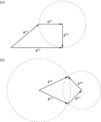
are potentially capable of exchanging energy with the waves via four-wave resonance (see figure 1). For example, consider the special case
 $\boldsymbol{k}^{W1}=\boldsymbol{k}^{W2}=\boldsymbol{k}$
,
 $\boldsymbol{k}^{G1}=\boldsymbol{k}^{\bot }$
and
 $\boldsymbol{k}^{G2}=\boldsymbol{k}^{\bot }+2\boldsymbol{k}$
, where
 $\boldsymbol{k}^{\bot }=\hat{\boldsymbol{z}}\times \boldsymbol{k}$
. For this system, (3.5) becomes
 $$\begin{eqnarray}\frac{\text{d}E_{G}}{\text{d}{\it\tau}}=8k^{4}h^{W1}h^{W2}h^{G1}h^{G2^{\ast }}+\text{c.c.}\end{eqnarray}$$
However, such an example is highly artificial and difficult to realize in practice, since an arbitrary set of two geostrophic modes will excite new geostrophic modes by triad interactions and transfer energy to those modes for time scales
 $T\sim O(1)$
. As a result, a simple set of four amplitude equations that demonstrate energetic interaction between waves and geostrophic modes does not seem plausible.
3.2. A special set of geostrophic modes
A special set of geostrophic modes that deserve attention are modes that satisfy
 $|\boldsymbol{k}^{G1}|^{2}=|\boldsymbol{k}^{G2}|^{2}$
. These geostrophic modes are special since in the absence of other modes they do not excite new geostrophic modes by triad interaction due to the fact that
 $\boldsymbol{v}_{G}\boldsymbol{\cdot }\boldsymbol{{\rm\nabla}}q_{0}=0$
for this set of modes (see appendix D for the proof). Thus, if we consider a system consisting of two such geostrophic modes and two wave modes of the same frequency (such that triad wave–geostrophic–wave interactions are absent), the leading nonlinear interactions would be quadruple interactions. The wave modes are expected to catalyse energy exchange between geostrophic modes in such a system. Of course, as follows from (3.5), these geostrophic modes will preserve their total energy.
We derive an example to demonstrate this mechanism by considering two waves (W1 and W2) and two geostrophic modes (G1 and G2). The waves are chosen from opposite branches but have the same wavenumber,
 $\boldsymbol{k}^{W1}=\boldsymbol{k}^{W2}=\boldsymbol{k}$
. The geostrophic modes have wavenumbers
 $\boldsymbol{k}^{G1}=2\boldsymbol{k}^{\bot }+\boldsymbol{k}$
and
 $\boldsymbol{k}^{G2}=2\boldsymbol{k}^{\bot }-\boldsymbol{k}$
. Such a set of wavenumbers with
 $\boldsymbol{k}$
as the only free parameter is a conscious choice to simplify the algebraic calculations involved in constructing the reduced system. For this special choice of two waves and two geostrophic modes there are no triad interactions. Since four-wave resonant interactions are expected to appear due to cubic nonlinearity at
 $O({\it\epsilon}^{2})$
in the asymptotic expansions, the slow time is chosen to be
 ${\it\tau}={\it\epsilon}^{2}t$
. The slowly evolving amplitude equations for these four modes are given by (details of the derivation are given in appendix E)
 $$\begin{eqnarray}\displaystyle & \displaystyle \frac{\text{d}h^{W1}}{\text{d}{\it\tau}}+\text{i}c_{ggw}h^{G1}h^{G2^{\ast }}h^{W2^{\ast }}+\text{i}(c_{ww}|h^{W1}|^{2}+c_{g1}|h^{G1}|^{2}+c_{g2}|h^{G2}|^{2})h^{W1}=0, & \displaystyle\end{eqnarray}$$
 $$\begin{eqnarray}\displaystyle & \displaystyle \frac{\text{d}h^{W2}}{\text{d}{\it\tau}}-\text{i}c_{ggw}h^{G1}h^{G2^{\ast }}h^{W1^{\ast }}-\text{i}(c_{ww}|h^{W2}|^{2}+c_{g1}|h^{G1}|^{2}+c_{g2}|h^{G2}|^{2})h^{W2}=0, & \displaystyle\end{eqnarray}$$
 $$\begin{eqnarray}\displaystyle & \displaystyle \frac{\text{d}h^{G1}}{\text{d}{\it\tau}}+c_{wwg}h^{G2}h^{W1}h^{W2}+c_{gg}|h^{G2}|^{2}h^{G1}=0, & \displaystyle\end{eqnarray}$$
 $$\begin{eqnarray}\displaystyle & \displaystyle \frac{\text{d}h^{G2}}{\text{d}{\it\tau}}-c_{wwg}h^{G1}h^{W1^{\ast }}h^{W2^{\ast }}-c_{gg}|h^{G1}|^{2}h^{G2}=0. & \displaystyle\end{eqnarray}$$
 $$\begin{eqnarray}\displaystyle \left.\begin{array}{@{}c@{}}c_{ggw}=4k^{2}(9k^{4}+2k^{2}-3)/3{\it\omega}^{3},\quad c_{ww}=3{\it\omega}k^{2},\\ c_{g1}=c_{g2}=(312k^{4}+128k^{2}-152)k^{2}/42{\it\omega}^{3},\\ c_{wwg}=4(k^{2}-3)k^{2}/(1+5k^{2}),\quad c_{gg}=-24k^{4}.\end{array}\right\} & & \displaystyle\end{eqnarray}$$
We then have the following energy equations from (3.7):
 $$\begin{eqnarray}\displaystyle \frac{\text{d}E^{W1}}{\text{d}{\it\tau}} & = & \displaystyle \frac{2\text{i}{\it\omega}^{2}c_{ggw}}{k^{2}}h^{G1^{\ast }}h^{G2}h^{W1}h^{W2}+\text{c.c.}=-\frac{\text{d}E^{W2}}{\text{d}{\it\tau}}\nonumber\\ \displaystyle & \Rightarrow & \displaystyle E_{W}=E^{W1}+E^{W2}=\frac{2{\it\omega}^{2}}{k^{2}}|h^{W1}|^{2}+\frac{2{\it\omega}^{2}}{k^{2}}|h^{W2}|^{2}=E_{W}(0),\end{eqnarray}$$
 $$\begin{eqnarray}\displaystyle \frac{\text{d}E^{G1}}{\text{d}{\it\tau}} & = & \displaystyle -(1+5k^{2})(c_{wwg}h^{G1^{\ast }}h^{G2}h^{W1}h^{W2}+c_{gg}|h^{G1}|^{2}|h^{G2}|^{2}+\text{c.c.})=-\frac{\text{d}E^{G2}}{\text{d}{\it\tau}}\nonumber\\ \displaystyle & \Rightarrow & \displaystyle E_{G}=E^{G1}+E^{G2}=(1+5k^{2})|h^{G1}|^{2}+(1+5k^{2})|h^{G2}|^{2}=E_{G}(0).\end{eqnarray}$$
 $$\begin{eqnarray}Q({\it\tau})=Q^{G1}+Q^{G2}=(1+5k^{2})^{2}|h^{G1}|^{2}+(1+5k^{2})^{2}|h^{G2}|^{2}=Q(0).\end{eqnarray}$$
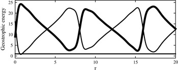
The main point we wish to make with the help of (3.7) is that the energetic interaction between balanced modes is affected by the presence of waves, although (3.7) conserves the total wave energy and total geostrophic energy separately. For an illustration of this, (3.7) is solved numerically using RK-4 for the initial conditions
 $h^{W1}=1,h^{W2}=2,h^{G1}=3,h^{G2}=4$
and
 $|\boldsymbol{k}|=1/4$
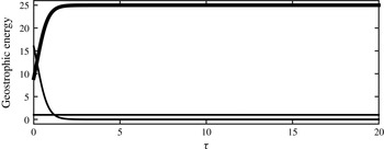
. Figure 2 shows the energy exchange between the geostrophic modes in the absence of waves, i.e. obtained by solving (3.7c,d
) after setting
 $c_{wwg}=0$
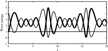
. It is seen that the G1 mode extracts all of the energy from G2, asymptotically gaining all of the energy in the system, while G2 asymptotes towards zero energy, leading to its demise. Figure 3 shows the effect of having waves in the system obtained by solving the complete system (3.7). In this case, the waves continuously transfer energy between the geostrophic modes in such a way that the G2 mode does not lose all of its energy to the G1 mode. As a minor point, we also observe that the geostrophic modes catalyse energy exchanges between the wave modes, as is shown in figure 4. (In the absence of the geostrophic modes, the waves do not interact, as may be inferred from (3.7a
) and (3.7b
).)
(a) The general case of quadruple interactions between waves and geostrophic modes in the absence of resonant triads. Two waves (W1 and W2) of the same frequency
 $(|\boldsymbol{k}^{W1}|^{2}=|\boldsymbol{k}^{W2}|^{2})$
can interact with two geostrophic modes (G1 and G2). The interaction can result in energy exchange between the waves and the geostrophic modes when
 $|\boldsymbol{k}^{G1}|^{2}\neq |\boldsymbol{k}^{G2}|^{2}$
. (b) A special case when
 $|\boldsymbol{k}^{G1}|^{2}=|\boldsymbol{k}^{G2}|^{2}$
. Geostrophic modes that fall into this category do not interact among themselves via triad interactions. In such a setting, the waves can catalyse energy exchange between the geostrophic modes, and the geostrophic modes can catalyse energy exchange between the waves. More specifically, the energetic interaction between geostrophic modes is modified by the presence of waves. However, there is no net transfer of energy between geostrophic modes and waves, i.e. the total geostrophic and total wave energies remain separately conserved.

Energy of the geostrophic modes (scaled by
 $1+5k^{2}$
) in the absence of wave modes. Thick and thin lines correspond to
 $|h^{G1}|^{2}$
and
 $|h^{G2}|^{2}$
respectively. The total geostrophic energy (scaled by the initial value) is conserved, as indicated by the straight line.

Energy of the geostrophic modes (scaled by
 $1+5k^{2}$
) in the presence of wave modes. Thick and thin lines correspond to
 $|h^{G1}|^{2}$
and
 $|h^{G2}|^{2}$
respectively. The total geostrophic energy (scaled by the initial value) is conserved, as indicated by the straight line.

Energy of the wave modes (scaled by
 $2{\it\omega}^{2}/k^{2}$
) in the presence of geostrophic modes. Thick and thin lines correspond to
 $|h^{W1}|^{2}$
and
 $|h^{W2}|^{2}$
respectively. The total wave energy (scaled by the initial value) is conserved, as indicated by the straight line.

4. Summary
This paper was aimed at investigating the evolution of unbalanced initial data in RSW in the regime
 $Ro\sim Fr\ll 1$
, with the main focus on interactions between slow balanced flow and fast waves. Using the method of multiple time scale asymptotic analysis, we derived an evolution equation for the slow dynamics of RSW valid for
 $t\lesssim 1/Ro^{2}$
, the well known classical QG equation being valid for
 $t\lesssim 1/Ro$
. Inertio-gravity waves were seen to influence the balanced flow, while spatially homogeneous inertial oscillations did not affect the geostrophic field up to
 $O(Ro^{2})$
. In the case of an unbounded domain with compact support for initial data, the wave-balanced flow interaction terms were seen to identically vanish due to fast decay of the wave amplitudes via dispersive propagation, in complete agreement with the results of RZB. In such a set-up, the process of geostrophic adjustment takes place and the slow balanced flow evolves unaffected by the fast modes, i.e quasi-geostrophy still holds, although the new governing equation is a higher-order balance equation (or an improved QG PV equation) with additional cubic nonlinear geostrophic interaction terms. However, in the case of a general domain that prevents dispersive propagation of waves and in the absence of dissipation (this may be real physical dissipation or artificial/numerical dissipation), the waves can influence the balanced flow. Furthermore, the energy equation corresponding to the slow evolution equation is not closed, implying that the slow dynamics can interact energetically with the fast modes. Thus, in the long-time limit, a splitting between fast and slow energy does not hold. Ertel potential enstrophy was shown to be an exact invariant of the higher-order slow evolution equation, although it contains contributions from the balanced part and the fast dynamics. Thus, fast–slow enstrophy exchanges are also possible in the long-time limit.
Hence, in the long-time limit,
 $t\gg 1/Ro$
, it is clear that an adjustment process leading to the slow evolution of the balanced flow uninfluenced by the fast fields is not possible and the QG framework of describing the evolution of balanced flow without information on wave dynamics breaks down. As a result, if the initial data are unbalanced, a slow manifold cannot exist in the long-time limit. Therefore, the central result of this work is that the slow dynamics obtained by filtering fast waves can deviate significantly from the slow dynamics obtained by tracking both fast and slow modes of the full parent model, which in this case is RSW. It is possible that the presence of wave activity influencing the geostrophic cascade as observed by Farge & Sadourny (Reference Farge and Sadourny1989) could be an indication of the early stages of interaction between the waves and the balanced flow. Significant interactions might occur if the dynamics were investigated for longer times with near-inviscid conditions, i.e. in a setting such that numerical dissipation does not considerably affect the dynamics for time scales of the order
 $t\sim 1/Ro^{2}$
.
The interaction was further investigated in a periodic domain with the goal of constructing a reduced system of slowly evolving amplitude equations. In the long-time limit,
 $t\sim 1/Ro^{2}$
, significant four-wave resonant interactions are expected to take place. In a system consisting of four modes (chosen such that there are no resonant triads in the system), two waves of the same frequency and two arbitrary geostrophic modes, the total geostrophic energy is not conserved but is exchanged with the fast waves. However, two arbitrary geostrophic modes in general do not form a closed system and can resonantly excite new geostrophic modes by triad interaction. A special case of non-resonant geostrophic modes, i.e. modes that do not excite new geostrophic modes via triad interactions, was chosen to derive the reduced system. Although the total geostrophic energy is conserved in such a system, the presence of waves modifies the energy exchange between the geostrophic modes. That is, the energetic interaction between balanced modes can be very greatly modified in the presence of waves, as was illustrated with a particular example. The geostrophic modes also act as catalysts for energetic interaction between the waves, although the total wave energy is also separately conserved in this reduced system. However, this reduced system only serves as a special example to illustrate that significant fast–slow interactions are possible in the long-time limit. High-accuracy numerical solutions of RSW will have to be undertaken to investigate the long-time state of unbalanced initial data.
Acknowledgements
The author acknowledges the Geophysical Fluid Dynamics – 2014 summer programme at Woods Hole Oceanographic Institution where some of the preliminary analysis that led to this paper was carried out. S. Smith is thanked for interesting discussions on the wave-balanced flow interaction problem, with a focus on periodic domains to investigate the long-time dynamics, for encouraging the author to write this paper and also for useful comments on an earlier version of this paper. The author is indebted to I. Grooms for pointing out some inaccuracies in the first draft and for helping to revise some of the early versions of this paper with critical but constructive comments and suggestions. O. Bühler is thanked for comments and suggestions that helped in the revision of an earlier draft. Three anonymous reviewers are also gratefully acknowledged for comments and suggestions that led to significant improvement of the paper.
Appendix A. Equivalence of two methods of multi-time-scale asymptotic analysis
Here, we show that the asymptotic technique that we used to derive the higher-order slow evolution equation of RSW using a single slow time scale, following Ablowitz (Reference Ablowitz2011), is equivalent to a method that uses two slow time scales. Consider a weakly nonlinear system of the form
 $$\begin{eqnarray}\frac{\partial u}{\partial t}+\mathscr{L}u+{\it\epsilon}\mathscr{B}(u,u)+{\it\epsilon}^{2}\mathscr{N}(u)=0,\end{eqnarray}$$
where
 $u\in \mathbb{R}$
,
 $\mathscr{L}$
is a linear self-adjoint operator,
 $\mathscr{B}(u,u)$
is a bilinear operator and
 $\mathscr{N}(u)$
is an arbitrary nonlinear operator acting on
 $u$
– these operators may be algebraic or differential (although here we restrict ourselves to the case of
 $u$
being a scalar field, all of these ideas may be easily extended to higher dimensions).
Two slow time scales
We introduce two slow times
 $T={\it\epsilon}t$
and
 ${\it\tau}={\it\epsilon}^{2}t$
to rewrite (A 1) as
 $$\begin{eqnarray}\frac{\partial u}{\partial t}+{\it\epsilon}\frac{\partial u}{\partial T}+{\it\epsilon}^{2}\frac{\partial u}{\partial {\it\tau}}+\mathscr{L}u+{\it\epsilon}\mathscr{B}(u,u)+{\it\epsilon}^{2}\mathscr{N}(u)=0.\end{eqnarray}$$
Using an asymptotic expansion of the form
 $u=u_{0}+{\it\epsilon}u_{1}+{\it\epsilon}^{2}u_{2}+\cdots \,$
, we write the leading-order solution of (A 2) as
 $u_{0}=\text{e}^{-\mathscr{L}t}U(T,{\it\tau})$
, where
 $\text{e}^{-\mathscr{L}t}$
is the linear solution in abstract form, with
 $\mathscr{L}$
being an algebraic or differential operator and
 $U(T,{\it\tau})$
being the slowly evolving amplitude. At
 $O({\it\epsilon})$
we obtain
 $$\begin{eqnarray}\frac{\partial u_{1}}{\partial t}+\mathscr{L}u_{1}=-\!\left\{\frac{\partial u_{0}}{\partial T}+\mathscr{B}(u_{0},u_{0})\!\right\}.\end{eqnarray}$$
We use the solvability condition to suppress secular growth of
 $u_{1}$
and obtain the slow evolution equation valid for
 $T\sim 1$
(
 $t\sim 1/{\it\epsilon}$
),
 $$\begin{eqnarray}\frac{\partial U}{\partial T}+\mathscr{R}\{\mathscr{B}(u_{0},u_{0})\}=0,\end{eqnarray}$$
where
 $\mathscr{R}({\it\psi})$
is the projection of
 ${\it\psi}$
on the linear solution
 $\text{e}^{-\mathscr{L}t}$
, i.e.
 $$\begin{eqnarray}\mathscr{R}\{{\it\psi}(\boldsymbol{x},t,T)\}=\lim _{\tilde{T}\rightarrow \infty }\frac{1}{\tilde{T}}\int _{0}^{\tilde{T}}\text{e}^{\mathscr{L}t}{\it\psi}(\boldsymbol{x},t,T)\,\text{d}t.\end{eqnarray}$$
By deriving (A 4), we have filtered the fast-time (
 $t\sim 1$
) dynamics from the leading-order solution, a process that is accompanied by several advantages. For example, numerical solution of (A 4) can use larger time steps than those allowed by (A 1). After removing the resonant terms, we can solve (A 3) to obtain
 $u_{1}$
. At
 $O({\it\epsilon}^{2})$
of (A 2), we obtain
 $$\begin{eqnarray}\frac{\partial u_{2}}{\partial t}+\mathscr{L}u_{2}=-\!\left\{\frac{\partial u_{1}}{\partial T}+\frac{\partial u_{0}}{\partial {\it\tau}}+\mathscr{B}(u_{0},u_{1})+\mathscr{B}(u_{1},u_{0})+\mathscr{N}(u_{0})\right\},\end{eqnarray}$$
where
 $\mathscr{B}(u_{0},u_{1})+\mathscr{B}(u_{1},u_{0})$
represent the terms that arise due to interactions between
 $u_{0}$
and
 $u_{1}$
in abstract form. We use the solvability condition again to eliminate
 $t$
dependence and obtain the second slow equation valid up to
 ${\it\tau}\sim 1$
(
 $t\sim 1/{\it\epsilon}^{2}$
),
 $$\begin{eqnarray}\frac{\partial U}{\partial {\it\tau}}+\mathscr{R}\left\{\frac{\partial u_{1}}{\partial T}+\mathscr{B}(u_{0},u_{1})+\mathscr{B}(u_{1},u_{0})+\mathscr{N}(u_{0})\right\}=0.\end{eqnarray}$$
Equation (A 7) has variables that evolve on two time scales –
 $T$
and
 ${\it\tau}$
. The
 $T$
dependence appears above since (1)
 $u_{1}$
obtained by solving (A 3) (after removing resonant terms) depends on
 $u_{0}$
; (2) nonlinear interactions,
 $\mathscr{B}(u_{0},u_{1})$
,
 $\mathscr{B}(u_{1},u_{0})$
and
 $N(u_{0})$
, have
 $T$
dependence,
 $u_{0}$
depending on
 $T$
as given by (A 4). Equation (A 7) is thus coupled to (A 4). In general, writing an evolution equation for the leading-order field valid for
 ${\it\tau}\sim 1$
, with the first slow time dependence removed, is a formidable task. Most of the difficulty arises because (A 4) is in general nonlinear and hence difficult to treat exactly. In short, constructing a solvability condition based on (A 4) and using it in (A 7) to filter off
 $T$
dependence, along the same lines that we adopted in passing from (A 3) to (A 4), is often difficult, except for some special solvable forms of (A 4). In hindsight this is hardly surprising, since we were able to introduce the solvability condition in (A 3) simply because the leading-order equation was linear, due to which we wrote down an exact solution to it. Once we encounter a nonlinear equation at higher order in asymptotics, such as (A 4), except for special cases, exact treatment is not easy.
A pragmatic strategy that bypasses all of these difficulties is to combine the two slow equations and write a single equation that holds for
 $T\sim 1$
to
 $T\sim 1/{\it\epsilon}$
. This is done by summing (A 4)
 $+$
 ${\it\epsilon}$
(A 7) and defining
 $\partial /\partial T+{\it\epsilon}\partial /\partial {\it\tau}\rightarrow \partial /\partial T$
, which gives a slow equation
 $$\begin{eqnarray}\frac{\partial U}{\partial T}+\mathscr{R}\{\mathscr{B}(u_{0},u_{0})\}+{\it\epsilon}\mathscr{R}\left\{\frac{\partial u_{1}}{\partial T}+\mathscr{B}(u_{0},u_{1})+\mathscr{B}(u_{1},u_{0})+\mathscr{N}(u_{0})\right\}=0,\end{eqnarray}$$
which is valid for
 $T\sim 1/{\it\epsilon}$
or
 $t\sim 1/{\it\epsilon}^{2}$
. At this point, one must realize that we have given up the idea of distinguishing between two slow time scales,
 $T$
and
 ${\it\tau}$
. Instead, a single slow time
 $T$
is allowed to vary from
 $O(1)$
to
 $O(1/{\it\epsilon})$
in (A 8). However, it must be noted that in spite of (A 8) containing
 ${\it\epsilon}$
, one is at a higher advantage solving (A 8) than solving (A 1) (up to
 $t\sim 1/{\it\epsilon}^{2}$
), which has fast dynamics
 $t\sim 1$
and hence requires very small time steps. Although the impact of the higher-order terms, i.e. terms multiplied by
 ${\it\epsilon}$
, is weak for
 $T\sim O(1)$
time scales, these terms may change the leading-order field by a significant amount in longer time scales,
 $T\sim 1/{\it\epsilon}$
.
A single slow time scale
We now show that one may obtain (A 8) by using a single slow time, i.e. without explicitly introducing two slow time scales, but by modifying the analysis slightly. We introduce a single slow time
 $T={\it\epsilon}t$
and rewrite (A 2) as
 $$\begin{eqnarray}\frac{\partial u}{\partial t}+{\it\epsilon}\frac{\partial u}{\partial T}+\mathscr{L}u+{\it\epsilon}\mathscr{B}(u,u)+{\it\epsilon}^{2}\mathscr{N}(u)=0.\end{eqnarray}$$
At
 $O({\it\epsilon})$
we rewrite (A 4) as
 $$\begin{eqnarray}\frac{\partial U}{\partial T}+\mathscr{R}\{\mathscr{B}(u_{0},u_{0})\}={\it\epsilon}{\it\Phi}(\boldsymbol{x},T)+O({\it\epsilon}^{2}),\end{eqnarray}$$
where
 ${\it\Phi}$
is a higher-order correction term and will be obtained at the next order. We also retain
 $O({\it\epsilon}^{2})$
on the right-hand side of the above equation to indicate the order of error terms involved and hence to imply that (A 10) is valid for
 $T\lesssim 1/{\it\epsilon}$
but not for
 $T\gg 1/{\it\epsilon}$
. At
 $O({\it\epsilon}^{2})$
of asymptotics we obtain
 $$\begin{eqnarray}\frac{\partial u_{2}}{\partial t}+\mathscr{L}u_{2}=-\!\left\{\frac{\partial u_{1}}{\partial T}+\text{e}^{-\mathscr{L}t}{\it\Phi}(\boldsymbol{x},T)+\mathscr{B}(u_{0},u_{1})+\mathscr{B}(u_{1},u_{0})+\mathscr{N}(u_{0})\right\}.\end{eqnarray}$$
Suppressing secular growth, we obtain
 $$\begin{eqnarray}{\it\Phi}(\boldsymbol{x},T)+\mathscr{R}\left\{\frac{\partial u_{1}}{\partial T}+\mathscr{B}(u_{0},u_{1})+\mathscr{B}(u_{1},u_{0})+\mathscr{N}(u_{0})\right\}=0.\end{eqnarray}$$
We combine (A 10) and (A 12) to obtain
 $$\begin{eqnarray}\frac{\partial U}{\partial T}+\mathscr{R}\{\mathscr{B}(u_{0},u_{0})\}+{\it\epsilon}\mathscr{R}\left\{\frac{\partial u_{1}}{\partial T}+\mathscr{B}(u_{0},u_{1})+\mathscr{B}(u_{1},u_{0})+\mathscr{N}(u_{0})\right\}+O({\it\epsilon}^{2})=0.\end{eqnarray}$$
Equation (A 13) is the slow equation valid for
 $t\sim 1/{\it\epsilon}^{2}$
, since we eliminated secular growth up to
 $O({\it\epsilon}^{2})$
. It should be noted that this is the same equation we obtained using two time scale asymptotics (A 8). Alternatively, if we redefine the time derivative in (A 13) as
 $\partial /\partial T\rightarrow \partial /\partial T+{\it\epsilon}\partial /\partial {\it\tau}$
and write the corresponding equations at
 $O(1)$
and
 $O({\it\epsilon})$
, we obtain (A 4) and (A 7). One may use (A 10) to modify the part of (A 13) multiplied by
 ${\it\epsilon}$
. The error involved in the process is
 $O({\it\epsilon}^{2})$
and is insignificant for
 $T\lesssim 1/{\it\epsilon}$
. This technique of using a single slow time and eliminating resonance up to
 $O({\it\epsilon}^{2})$
to derive a slow equation for RSW valid up to
 $t\sim 1/{\it\epsilon}^{2}$
was adopted in this paper. The reader may refer to Ablowitz (Reference Ablowitz2011) for particular examples that take advantage of this method.
Appendix B. Higher-order balance equation
Here, we show that the higher-order balance equation we derived in the absence of waves, (2.24), is equivalent to the improved QG PV equation of RZB.
We ignore waves (i.e. set
 $\boldsymbol{v}_{W}=h_{W}=0$
) and use
 $\hat{\boldsymbol{z}}\times {\it\zeta}_{G}\boldsymbol{v}_{G}+\boldsymbol{{\rm\nabla}}(v_{G}^{2}/2)=\boldsymbol{v}_{G}\boldsymbol{\cdot }\boldsymbol{{\rm\nabla}}\boldsymbol{v}_{G}$
in (2.12a
) to obtain an alternate form of (2.13c
),
 $$\begin{eqnarray}\displaystyle & \displaystyle {\overline{\boldsymbol{v}}_{1}}_{G}=-\boldsymbol{{\rm\nabla}}\frac{\partial h_{G}}{\partial T}+\hat{\boldsymbol{z}}\times \boldsymbol{{\rm\nabla}}\overline{h}_{1}-(\boldsymbol{v}_{G}\boldsymbol{\cdot }\boldsymbol{{\rm\nabla}})(\boldsymbol{{\rm\nabla}}h_{G}) & \displaystyle\end{eqnarray}$$
 $$\begin{eqnarray}\displaystyle & \displaystyle \Rightarrow \quad {\overline{q}_{1}}_{G}=\hat{\boldsymbol{z}}\boldsymbol{\cdot }(\boldsymbol{{\rm\nabla}}\times {\overline{\boldsymbol{v}}_{1}}_{G})-\overline{h}_{1}=({\it\Delta}-1)\overline{h}_{1}-2\partial [{h_{G}}_{x},{h_{G}}_{y}], & \displaystyle\end{eqnarray}$$
 $\partial [f,g]=f_{x}g_{y}-f_{y}g_{x}$
. Now,
 $$\begin{eqnarray}\displaystyle \boldsymbol{{\rm\nabla}}\boldsymbol{\cdot }(q_{0}{\overline{\boldsymbol{v}}_{1}}_{G}) & = & \displaystyle -q_{0}\frac{\partial h_{G}}{\partial T}+{\overline{\boldsymbol{v}}_{1}}_{G}\boldsymbol{\cdot }\boldsymbol{{\rm\nabla}}q_{0}\nonumber\\ \displaystyle & & \displaystyle (\text{using a modified form of (2.13d)},\boldsymbol{{\rm\nabla}}\boldsymbol{\cdot }{\overline{\boldsymbol{v}}_{1}}_{G}=-\partial h_{G}/\partial T)\nonumber\\ \displaystyle & = & \displaystyle -\frac{\partial }{\partial T}(q_{0}h_{G})+h_{G}\frac{\partial q_{0}}{\partial T}+(\hat{\boldsymbol{z}}\times \boldsymbol{{\rm\nabla}}\overline{h}_{1})\boldsymbol{\cdot }\boldsymbol{{\rm\nabla}}q_{0}-\boldsymbol{{\rm\nabla}}q_{0}\boldsymbol{\cdot }\frac{\partial }{\partial T}(\boldsymbol{{\rm\nabla}}h_{G})\nonumber\\ \displaystyle & & \displaystyle -\,\boldsymbol{{\rm\nabla}}q_{0}\boldsymbol{\cdot }\{(\boldsymbol{v}_{G}\boldsymbol{\cdot }\boldsymbol{{\rm\nabla}})\boldsymbol{{\rm\nabla}}h_{G}\}\quad (\text{using (B 1a)})\nonumber\\ \displaystyle & = & \displaystyle -\frac{\partial }{\partial T}(q_{0}h_{G})-h_{G}\boldsymbol{{\rm\nabla}}\boldsymbol{\cdot }(q_{0}\boldsymbol{v}_{G})+(\hat{\boldsymbol{z}}\times \boldsymbol{{\rm\nabla}}\overline{h}_{1})\boldsymbol{\cdot }\boldsymbol{{\rm\nabla}}q_{0}-\frac{\partial }{\partial T}\{\boldsymbol{{\rm\nabla}}q_{0}\boldsymbol{\cdot }\boldsymbol{{\rm\nabla}}h_{G}\}\nonumber\\ \displaystyle & & \displaystyle +\,\left\{\boldsymbol{{\rm\nabla}}h_{G}\boldsymbol{\cdot }\frac{\partial }{\partial T}\boldsymbol{{\rm\nabla}}q_{0}-\boldsymbol{{\rm\nabla}}q_{0}\boldsymbol{\cdot }\{(\boldsymbol{v}_{G}\boldsymbol{\cdot }\boldsymbol{{\rm\nabla}})\boldsymbol{{\rm\nabla}}h_{G}\}\right\}+O({\it\epsilon})\nonumber\\ \displaystyle & & \displaystyle (\text{using (2.17)})\nonumber\\ \displaystyle & = & \displaystyle -\frac{\partial }{\partial T}(q_{0}h_{G}+\boldsymbol{{\rm\nabla}}q_{0}\boldsymbol{\cdot }\boldsymbol{{\rm\nabla}}h_{G})-\boldsymbol{{\rm\nabla}}\boldsymbol{\cdot }(h_{G}q_{0}\boldsymbol{v}_{G})+(\hat{\boldsymbol{z}}\times \boldsymbol{{\rm\nabla}}\overline{h}_{1})\boldsymbol{\cdot }\boldsymbol{{\rm\nabla}}q_{0}\nonumber\\ \displaystyle & & \displaystyle -\,[\boldsymbol{{\rm\nabla}}h_{G}\boldsymbol{\cdot }\boldsymbol{{\rm\nabla}}(\boldsymbol{v}_{G}\boldsymbol{\cdot }\boldsymbol{{\rm\nabla}}q_{0})+\boldsymbol{{\rm\nabla}}q_{0}\boldsymbol{\cdot }\{(\boldsymbol{v}_{G}\boldsymbol{\cdot }\boldsymbol{{\rm\nabla}})\boldsymbol{{\rm\nabla}}h_{G}\}]+O({\it\epsilon})\nonumber\\ \displaystyle & & \displaystyle (\text{using (2.17) again}).\end{eqnarray}$$
After some manipulations, one can show that
 $$\begin{eqnarray}\displaystyle \boldsymbol{{\rm\nabla}}h_{G}\boldsymbol{\cdot }\boldsymbol{{\rm\nabla}}(\boldsymbol{v}_{G}\boldsymbol{\cdot }\boldsymbol{{\rm\nabla}}q_{0})=\boldsymbol{{\rm\nabla}}h_{G}\boldsymbol{\cdot }(\boldsymbol{v}_{G}\boldsymbol{\cdot }\boldsymbol{{\rm\nabla}})\boldsymbol{{\rm\nabla}}q_{0}+\left\{\hat{\boldsymbol{z}}\times \boldsymbol{{\rm\nabla}}\left({\textstyle \frac{1}{2}}(\boldsymbol{{\rm\nabla}}h_{G})^{2}\right)\right\}\boldsymbol{\cdot }\boldsymbol{{\rm\nabla}}q_{0}. & & \displaystyle\end{eqnarray}$$
Substituting (B 3) in (B 2) gives
 $$\begin{eqnarray}\displaystyle \boldsymbol{{\rm\nabla}}\boldsymbol{\cdot }(q_{0}{\overline{\boldsymbol{v}}_{1}}_{G}) & = & \displaystyle -\frac{\partial }{\partial T}(q_{0}h_{G}+\boldsymbol{{\rm\nabla}}q_{0}\boldsymbol{\cdot }\boldsymbol{{\rm\nabla}}h_{G})-\boldsymbol{{\rm\nabla}}\boldsymbol{\cdot }(h_{G}q_{0}\boldsymbol{v}_{G})+\partial [\overline{h}_{1},q_{0}]\nonumber\\ \displaystyle & & \displaystyle -\,(\boldsymbol{v}_{G}\boldsymbol{\cdot }\boldsymbol{{\rm\nabla}})(\boldsymbol{{\rm\nabla}}q_{0}\boldsymbol{\cdot }\boldsymbol{{\rm\nabla}}h_{G})-\partial \left[\frac{1}{2}(\boldsymbol{{\rm\nabla}}h_{G})^{2},q_{0}\right]+O({\it\epsilon}).\end{eqnarray}$$
Substituting (B 1b ) and (B 4) in (2.24) and rearranging gives
 $$\begin{eqnarray}\displaystyle & & \displaystyle \frac{\partial Q}{\partial T}+\partial \left[\left\{(h_{G}+{\it\epsilon}\overline{h}_{1})-{\it\epsilon}\frac{1}{2}(\boldsymbol{{\rm\nabla}}h_{G})^{2}\right\},Q\right]+O({\it\epsilon}^{2})=0,\nonumber\\ \displaystyle & & \displaystyle \quad \text{where }Q=({\it\Delta}-1)(h_{G}+{\it\epsilon}\overline{h}_{1})-2{\it\epsilon}\partial [{h_{G}}_{x},{h_{G}}_{y}]-{\it\epsilon}q_{0}h_{G}-{\it\epsilon}\boldsymbol{{\rm\nabla}}q_{0}\boldsymbol{\cdot }\boldsymbol{{\rm\nabla}}h_{G}.\end{eqnarray}$$
One may further combine the slow height fields as
 $\overline{h}=h_{G}+{\it\epsilon}\overline{h}_{1}$
to rewrite the above equation as
 $$\begin{eqnarray}\displaystyle & & \displaystyle \hspace{-12.0pt}\frac{\partial Q}{\partial T}+\partial \left[\left\{\overline{h}-{\it\epsilon}\frac{1}{2}(\boldsymbol{{\rm\nabla}}\overline{h})^{2}\right\},Q\right]+O({\it\epsilon}^{2})=0,\nonumber\\ \displaystyle & & \displaystyle \hspace{-12.0pt}\quad \text{where }Q=({\it\Delta}-1)\overline{h}-2{\it\epsilon}\partial [\overline{h}_{x},\overline{h}_{y}]-{\it\epsilon}\overline{h}({\it\Delta}-1)\overline{h}-{\it\epsilon}\boldsymbol{{\rm\nabla}}\overline{h}\boldsymbol{\cdot }\boldsymbol{{\rm\nabla}}\{({\it\Delta}-1)\overline{h}\}+O({\it\epsilon}^{2}).\qquad\end{eqnarray}$$
The error involved in the operation is
 $O({\it\epsilon}^{2})$
, which is insignificant for time scales
 $T\lesssim O(1/{\it\epsilon})$
. The above equation is the improved QG PV equation (3.72) of RZB, which was also derived by Allen (Reference Allen1993) and Warn et al. (Reference Warn, Bokhove, Shepherd and Vallis1995).
Appendix C. Derivation of the slow energy equation
Here, we describe the steps leading to the slow energy equation, (2.35). We spatially average (2.34) to obtain
 $$\begin{eqnarray}\displaystyle & & \displaystyle \left\langle h_{G}\frac{\partial q_{0}}{\partial T}+{\it\epsilon}\frac{\partial }{\partial T}\{h_{G}({\overline{q}_{1}}_{G}+{\overline{q}_{1}}_{W})\}\right\rangle \nonumber\\ \displaystyle & & \displaystyle \quad -\,{\it\epsilon}\left\langle {\overline{q}_{1}}_{G}\frac{\partial h_{G}}{\partial T}+q_{0}\boldsymbol{{\rm\nabla}}h_{G}\boldsymbol{\cdot }{\overline{\boldsymbol{v}}_{1}}_{G}+{\overline{q}_{1}}_{W}\frac{\partial h_{G}}{\partial T}+q_{0}\boldsymbol{{\rm\nabla}}h_{G}\boldsymbol{\cdot }{\overline{\boldsymbol{v}}_{1}}_{W}+\overline{(\boldsymbol{{\rm\nabla}}h_{G}\boldsymbol{\cdot }\boldsymbol{v}_{W}){q_{1}^{\prime }}_{W}}\right\rangle \nonumber\\ \displaystyle & & \displaystyle \quad +\,O({\it\epsilon}^{2})=0.\end{eqnarray}$$
We now observe that
 $$\begin{eqnarray}\displaystyle h_{G}\frac{\partial q_{0}}{\partial T} & = & \displaystyle h_{G}\frac{\partial }{\partial T}({\it\Delta}h_{G}-h_{G})=-\frac{\partial }{\partial T}\left(\frac{\boldsymbol{v}_{G}^{2}}{2}+\frac{h_{G}^{2}}{2}\right)+\boldsymbol{{\rm\nabla}}\boldsymbol{\cdot }\left(h_{G}\boldsymbol{{\rm\nabla}}\frac{\partial h_{G}}{\partial T}\right)\nonumber\\ \displaystyle & \Rightarrow & \displaystyle \left\langle h_{G}\frac{\partial q_{0}}{\partial T}\right\rangle =-\!\frac{\partial }{\partial T}\left\langle \left(\frac{\boldsymbol{v}_{G}^{2}}{2}+\frac{h_{G}^{2}}{2}\right)\right\rangle .\end{eqnarray}$$
We use (2.14) to obtain
 $$\begin{eqnarray}\displaystyle h_{G}{\overline{q}_{1}}_{G} & = & \displaystyle \hat{\boldsymbol{z}}\boldsymbol{\cdot }(h_{G}\boldsymbol{{\rm\nabla}}\times {\overline{\boldsymbol{v}}_{1}}_{G})-h_{G}\overline{h}_{1}=\hat{\boldsymbol{z}}\boldsymbol{\cdot }\boldsymbol{{\rm\nabla}}\times (h_{G}{\overline{\boldsymbol{v}}_{1}}_{G})-\hat{\boldsymbol{z}}\boldsymbol{\cdot }(\boldsymbol{{\rm\nabla}}h_{G}\times {\overline{\boldsymbol{v}}_{1}}_{G})-h_{G}\overline{h}_{1}\nonumber\\ \displaystyle & = & \displaystyle \hat{\boldsymbol{z}}\boldsymbol{\cdot }\boldsymbol{{\rm\nabla}}\times (h_{G}{\overline{\boldsymbol{v}}_{1}}_{G})-(\boldsymbol{v}_{G}\boldsymbol{\cdot }{\overline{\boldsymbol{v}}_{1}}_{G}+h_{G}\overline{h}_{1})\nonumber\\ \displaystyle & \Rightarrow & \displaystyle \langle h_{G}{\overline{q}_{1}}_{G}\rangle =-\langle \boldsymbol{v}_{G}\boldsymbol{\cdot }{\overline{\boldsymbol{v}}_{1}}_{G}+h_{G}\overline{h}_{1}\rangle\end{eqnarray}$$
and
 $$\begin{eqnarray}\displaystyle h_{G}{\overline{q}_{1}}_{W} & = & \displaystyle \hat{\boldsymbol{z}}\boldsymbol{\cdot }(h_{G}\boldsymbol{{\rm\nabla}}\times {\overline{\boldsymbol{v}}_{1}}_{W})=\hat{\boldsymbol{z}}\boldsymbol{\cdot }\boldsymbol{{\rm\nabla}}\times (h_{G}{\overline{\boldsymbol{v}}_{1}}_{W})-\hat{\boldsymbol{z}}\boldsymbol{\cdot }(\boldsymbol{{\rm\nabla}}h_{G}\times {\overline{\boldsymbol{v}}_{1}}_{W})\nonumber\\ \displaystyle & = & \displaystyle \hat{\boldsymbol{z}}\boldsymbol{\cdot }\boldsymbol{{\rm\nabla}}\times (h_{G}{\overline{\boldsymbol{v}}_{1}}_{W})-\boldsymbol{v}_{G}\boldsymbol{\cdot }{\overline{\boldsymbol{v}}_{1}}_{W}\nonumber\\ \displaystyle & \Rightarrow & \displaystyle \langle h_{G}{\overline{q}_{1}}_{W}\rangle =-\langle \boldsymbol{v}_{G}\boldsymbol{\cdot }{\overline{\boldsymbol{v}}_{1}}_{W}\rangle .\end{eqnarray}$$
Equation (2.14c ) is used for
 $$\begin{eqnarray}\displaystyle \frac{\partial h_{G}}{\partial T}{\overline{q}_{1}}_{G} & = & \displaystyle \frac{\partial h_{G}}{\partial T}{\it\Delta}\overline{h}_{1}-\frac{\partial h_{G}}{\partial T}\overline{h}_{1}+\frac{\partial h_{G}}{\partial T}{\it\Delta}\left(\frac{\boldsymbol{v}_{G}^{2}}{2}\right)-\frac{\partial h_{G}}{\partial T}\boldsymbol{{\rm\nabla}}\boldsymbol{\cdot }({\it\zeta}_{G}\boldsymbol{{\rm\nabla}}h_{G})\nonumber\\ \displaystyle & = & \displaystyle \overline{h}_{1}{\it\Delta}\frac{\partial h_{G}}{\partial T}-\overline{h}_{1}\frac{\partial h_{G}}{\partial T}+\boldsymbol{{\rm\nabla}}\boldsymbol{\cdot }\left(\frac{\partial h_{G}}{\partial T}\boldsymbol{{\rm\nabla}}\overline{h}_{1}-\overline{h}_{1}\boldsymbol{{\rm\nabla}}\frac{\partial h_{G}}{\partial T}\right)+\left(\frac{\boldsymbol{v}_{G}^{2}}{2}\right){\it\Delta}\frac{\partial h_{G}}{\partial T}\nonumber\\ \displaystyle & & \displaystyle +\,\boldsymbol{{\rm\nabla}}\boldsymbol{\cdot }\left(\frac{\partial h_{G}}{\partial T}\boldsymbol{{\rm\nabla}}\left(\frac{\boldsymbol{v}_{G}^{2}}{2}\right)-\left(\frac{\boldsymbol{v}_{G}^{2}}{2}\right)\boldsymbol{{\rm\nabla}}\frac{\partial h_{G}}{\partial T}\right)\nonumber\\ \displaystyle & & \displaystyle -\,\boldsymbol{{\rm\nabla}}\boldsymbol{\cdot }\left({\it\zeta}_{G}\frac{\partial h_{G}}{\partial T}\boldsymbol{{\rm\nabla}}h_{G}\right)+{\it\zeta}_{G}\frac{\partial }{\partial T}\left(\frac{\boldsymbol{v}_{G}^{2}}{2}\right)\nonumber\\ \displaystyle & \Rightarrow & \displaystyle \left\langle \frac{\partial h_{G}}{\partial T}{\overline{q}_{1}}_{G}\right\rangle =\left\langle \overline{h}_{1}\frac{\partial q_{0}}{\partial T}+\frac{\partial }{\partial T}\left({\it\zeta}_{G}\frac{\boldsymbol{v}_{G}^{2}}{2}\right)\right\rangle\end{eqnarray}$$
and (2.13c ) is used to obtain
 $$\begin{eqnarray}\displaystyle q_{0}\boldsymbol{{\rm\nabla}}h_{G}\boldsymbol{\cdot }{\overline{\boldsymbol{v}}_{1}}_{G} & = & \displaystyle -q_{0}\boldsymbol{v}_{G}\boldsymbol{\cdot }\left\{\frac{\partial \boldsymbol{v}_{G}}{\partial T}+\boldsymbol{{\rm\nabla}}\left(\overline{h}_{1}+\frac{\boldsymbol{v}_{G}^{2}}{2}\right)\right\}\nonumber\\ \displaystyle & = & \displaystyle -q_{0}\frac{\partial }{\partial T}\left(\frac{\boldsymbol{v}_{G}^{2}}{2}\right)-\boldsymbol{{\rm\nabla}}\boldsymbol{\cdot }\left\{q_{0}\boldsymbol{v}_{G}\left(\overline{h}_{1}+\frac{\boldsymbol{v}_{G}^{2}}{2}\right)\right\}+\left(\overline{h}_{1}+\frac{\boldsymbol{v}_{G}^{2}}{2}\right)\boldsymbol{{\rm\nabla}}\boldsymbol{\cdot }(q_{0}\boldsymbol{v}_{G})\nonumber\\ \displaystyle & = & \displaystyle -\frac{\partial }{\partial T}\left(q_{0}\frac{\boldsymbol{v}_{G}^{2}}{2}\right)-\overline{h}_{1}\frac{\partial q_{0}}{\partial T}-\boldsymbol{{\rm\nabla}}\boldsymbol{\cdot }\left\{q_{0}\boldsymbol{v}_{G}\left(\overline{h}_{1}+\frac{\boldsymbol{v}_{G}^{2}}{2}\right)\right\}+O({\it\epsilon})\nonumber\\ \displaystyle & & \displaystyle \text{(using (2.17))}\nonumber\\ \displaystyle & \Rightarrow & \displaystyle \langle q_{0}\boldsymbol{{\rm\nabla}}h_{G}\boldsymbol{\cdot }{\overline{\boldsymbol{v}}_{1}}_{G}\rangle =-\left\langle \frac{\partial }{\partial T}\left(q_{0}\frac{\boldsymbol{v}_{G}^{2}}{2}\right)+\overline{h}_{1}\frac{\partial q_{0}}{\partial T}\right\rangle +O({\it\epsilon}).\end{eqnarray}$$
We use (2.14b ) for
 $$\begin{eqnarray}\displaystyle \frac{\partial h_{G}}{\partial T}{\overline{q}_{1}}_{W} & = & \displaystyle \frac{\partial h_{G}}{\partial T}{\it\Delta}\left(\frac{\overline{\boldsymbol{v}_{W}^{2}}}{2}\right)-\frac{\partial h_{G}}{\partial T}\overline{h_{W}^{2}}-\hat{\boldsymbol{z}}\boldsymbol{\cdot }\left(\overline{\boldsymbol{{\rm\nabla}}h_{W}\times \boldsymbol{v}_{W}}\frac{\partial h_{G}}{\partial T}\right)\nonumber\\ \displaystyle & = & \displaystyle \left(\frac{\overline{\boldsymbol{v}_{W}^{2}}}{2}\right)\frac{\partial }{\partial T}{\rm\Delta}h_{G}+\boldsymbol{{\rm\nabla}}\boldsymbol{\cdot }\left(\frac{\partial h_{G}}{\partial T}\boldsymbol{{\rm\nabla}}\left(\frac{\overline{\boldsymbol{v}_{W}^{2}}}{2}\right)-\left(\frac{\overline{\boldsymbol{v}_{W}^{2}}}{2}\right)\boldsymbol{{\rm\nabla}}\frac{\partial h_{G}}{\partial T}\right)-\frac{\partial h_{G}}{\partial T}\overline{h_{W}^{2}}\nonumber\\ \displaystyle & & \displaystyle -\,\left\{\hat{\boldsymbol{z}}\boldsymbol{\cdot }\boldsymbol{{\rm\nabla}}\times \left(\frac{\partial h_{G}}{\partial T}\overline{h_{W}\boldsymbol{v}_{W}}\right)-\frac{\partial h_{G}}{\partial T}\overline{h_{W}^{2}}-\frac{\partial \boldsymbol{v}_{G}}{\partial T}\boldsymbol{\cdot }\overline{h_{W}\boldsymbol{v}_{W}}\right\}\nonumber\\ \displaystyle & \Rightarrow & \displaystyle \left\langle \frac{\partial h_{G}}{\partial T}{\overline{q}_{1}}_{W}\right\rangle =\left\langle \left(\frac{\overline{\boldsymbol{v}_{W}^{2}}}{2}\right)\frac{\partial {\it\zeta}_{G}}{\partial T}+\frac{\partial \boldsymbol{v}_{G}}{\partial T}\cdot \overline{h_{W}\boldsymbol{v}_{W}}\right\rangle\end{eqnarray}$$
and (2.13b ) to obtain
 $$\begin{eqnarray}\displaystyle \boldsymbol{{\rm\nabla}}h_{G}\boldsymbol{\cdot }q_{0}{\overline{\boldsymbol{v}}_{1}}_{W} & = & \displaystyle -q_{0}\boldsymbol{{\rm\nabla}}h_{G}\boldsymbol{\cdot }\overline{h_{W}\boldsymbol{v}_{W}}-q_{0}\boldsymbol{v}_{G}\boldsymbol{\cdot }\boldsymbol{{\rm\nabla}}\left(\frac{\overline{\boldsymbol{v}_{W}^{2}}}{2}\right)\nonumber\\ \displaystyle & = & \displaystyle -q_{0}\boldsymbol{{\rm\nabla}}h_{G}\boldsymbol{\cdot }\overline{h_{W}\boldsymbol{v}_{W}}+\left(\frac{\overline{\boldsymbol{v}_{W}^{2}}}{2}\right)\boldsymbol{{\rm\nabla}}\boldsymbol{\cdot }(q_{0}\boldsymbol{v}_{G})-\boldsymbol{{\rm\nabla}}\boldsymbol{\cdot }\left(q_{0}\boldsymbol{v}_{G}\frac{\overline{\boldsymbol{v}_{W}^{2}}}{2}\right)\nonumber\\ \displaystyle & \Rightarrow & \displaystyle \langle \boldsymbol{{\rm\nabla}}h_{G}\boldsymbol{\cdot }q_{0}{\overline{\boldsymbol{v}}_{1}}_{W}\rangle =-\left\langle q_{0}\boldsymbol{{\rm\nabla}}h_{G}\boldsymbol{\cdot }\overline{h_{W}\boldsymbol{v}_{W}}+\frac{\partial q_{0}}{\partial T}\left(\frac{\overline{\boldsymbol{v}_{W}^{2}}}{2}\right)\right\rangle +O({\it\epsilon}),\quad\end{eqnarray}$$
where we used (2.17). Finally, we use (2.16b ) to obtain
 $$\begin{eqnarray}\displaystyle \overline{(\boldsymbol{{\rm\nabla}}h_{G}\boldsymbol{\cdot }\boldsymbol{v}_{W}){q_{1}^{\prime }}_{W}}=q_{0}\boldsymbol{{\rm\nabla}}h_{G}\boldsymbol{\cdot }\overline{(h_{W}\boldsymbol{v}_{W})}-\overline{(\boldsymbol{{\rm\nabla}}h_{G}\boldsymbol{\cdot }\boldsymbol{v}_{W})\boldsymbol{{\rm\nabla}}q_{0}\boldsymbol{\cdot }\int ^{t}\boldsymbol{v}_{W}\,\text{d}t}. & & \displaystyle\end{eqnarray}$$
Substituting (C 2)–(C 9) in (C 1) and simplifying gives the energy equation (2.35).
Appendix D. Non-resonant geostrophic modes in the periodic domain
Here, we prove that geostrophic modes having the same wavenumber vector magnitude do not excite new modes via triad interaction since
 $\boldsymbol{v}_{G}\boldsymbol{\cdot }\boldsymbol{{\rm\nabla}}q=0$
for these modes. We note that for a particular mode,
 $$\begin{eqnarray}\displaystyle & \displaystyle q=({\it\Delta}-1)h_{G}\Rightarrow q_{k}=-(1+|\boldsymbol{k}|^{2})h_{k}, & \displaystyle\end{eqnarray}$$
 $$\begin{eqnarray}\displaystyle & \displaystyle \boldsymbol{v}_{G}=\hat{\boldsymbol{z}}\times \boldsymbol{{\rm\nabla}}h_{G}\Rightarrow \boldsymbol{v}_{k}=\text{i}h_{k}\boldsymbol{k}^{\bot }. & \displaystyle\end{eqnarray}$$
 $(\boldsymbol{v}_{G},q)=(\boldsymbol{v}_{1},q_{1})\text{e}^{\boldsymbol{k}_{1}\boldsymbol{\cdot }\boldsymbol{x}}+(\boldsymbol{v}_{2},q_{2})\text{e}^{\boldsymbol{k}_{2}\boldsymbol{\cdot }\boldsymbol{x}}+\text{c.c.}$
Then,
 $$\begin{eqnarray}\displaystyle & & \displaystyle \boldsymbol{v}_{G}\boldsymbol{\cdot }\boldsymbol{{\rm\nabla}}q\nonumber\\ \displaystyle & & \displaystyle \quad =\text{i}\{(\boldsymbol{k}_{1}\boldsymbol{\cdot }\boldsymbol{v}_{2})q_{1}+(\boldsymbol{k}_{2}\boldsymbol{\cdot }\boldsymbol{v}_{1})q_{2}\}\text{e}^{\text{i}(\boldsymbol{k}_{1}+\boldsymbol{k}_{2})\boldsymbol{\cdot }\boldsymbol{x}}+\text{i}\{(\boldsymbol{k}_{1}\boldsymbol{\cdot }\boldsymbol{v}_{2}^{\ast })q_{1}-(\boldsymbol{k}_{2}\boldsymbol{\cdot }\boldsymbol{v}_{1})q_{2}^{\ast }\}\text{e}^{\text{i}(\boldsymbol{k}_{1}-\boldsymbol{k}_{2})\boldsymbol{\cdot }\boldsymbol{x}}+\text{c.c.}\nonumber\\ \displaystyle & & \displaystyle \quad =-\{(|\boldsymbol{k}_{1}|^{2}-|\boldsymbol{k}_{2}|^{2})(\boldsymbol{k}_{1}\boldsymbol{\cdot }\boldsymbol{k}_{2}^{\bot })\}\{h_{1}h_{2}\text{e}^{\text{i}(\boldsymbol{k}_{1}+\boldsymbol{k}_{2})\boldsymbol{\cdot }\boldsymbol{x}}-h_{1}h_{2}^{\ast }\text{e}^{\text{i}(\boldsymbol{k}_{1}-\boldsymbol{k}_{2})\boldsymbol{\cdot }\boldsymbol{x}}\}+\text{c.c.},\end{eqnarray}$$
where we used (D 2). Thus, there will be no triad interactions, and
 $\boldsymbol{v}_{G}\boldsymbol{\cdot }\boldsymbol{{\rm\nabla}}q=0$
if
 $$\begin{eqnarray}|\boldsymbol{k}_{1}|^{2}=|\boldsymbol{k}_{2}|^{2}\quad \text{or }\boldsymbol{k}_{1}=c\boldsymbol{k}_{2},\end{eqnarray}$$
where
 $c$
is an arbitrary constant.
Appendix E. Derivation of the amplitude equations for quadruple wave-balanced mode interactions
We derive amplitude equations for a system consisting of two geostrophic and two wave modes. Since we will not encounter triad interactions for this reduced system, we let the slow time be
 ${\it\tau}={\it\epsilon}^{2}t$
and rewrite (2.2) as
 $$\begin{eqnarray}\displaystyle & \displaystyle \frac{\partial \boldsymbol{v}}{\partial t}+\hat{\boldsymbol{z}}\times \boldsymbol{v}+\boldsymbol{{\rm\nabla}}h+{\it\epsilon}\boldsymbol{v}\boldsymbol{\cdot }\boldsymbol{{\rm\nabla}}\boldsymbol{v}+{\it\epsilon}^{2}\frac{\partial \boldsymbol{v}}{\partial {\it\tau}}=0, & \displaystyle\end{eqnarray}$$
 $$\begin{eqnarray}\displaystyle & \displaystyle \frac{\partial h}{\partial t}+\boldsymbol{{\rm\nabla}}\boldsymbol{\cdot }\boldsymbol{v}+{\it\epsilon}\boldsymbol{{\rm\nabla}}\boldsymbol{\cdot }(h\boldsymbol{v})+{\it\epsilon}^{2}\frac{\partial h}{\partial {\it\tau}}=0, & \displaystyle\end{eqnarray}$$
 $$\begin{eqnarray}\displaystyle & \displaystyle \frac{\partial q}{\partial t}+{\it\epsilon}\boldsymbol{{\rm\nabla}}\boldsymbol{\cdot }(q\boldsymbol{v})+{\it\epsilon}^{2}\frac{\partial q}{\partial {\it\tau}}=0. & \displaystyle\end{eqnarray}$$
 $O(1)$
equations
Equations (2.5) form the
 $O(1)$
equations. We write the solution of this system as
 $$\begin{eqnarray}\displaystyle (\boldsymbol{v}_{0},h_{0}) & = & \displaystyle (\boldsymbol{v}^{G1},h^{G1})\exp \{\text{i}(2\boldsymbol{k}^{\bot }+\boldsymbol{k})\boldsymbol{\cdot }\boldsymbol{x}\}+(\boldsymbol{v}^{G2},h^{G2})\exp \{\text{i}(2\boldsymbol{k}^{\bot }-\boldsymbol{k})\boldsymbol{\cdot }\boldsymbol{x}\}\nonumber\\ \displaystyle & & \displaystyle +\,(\boldsymbol{v}^{W1},h^{W1})\exp \{\text{i}(\boldsymbol{k}\boldsymbol{\cdot }\boldsymbol{x}-{\it\omega}t)\}+(\boldsymbol{v}^{W2},h^{W2})\exp \{\text{i}(\boldsymbol{k}\boldsymbol{\cdot }\boldsymbol{x}+{\it\omega}t)\}+\text{c.c.}\qquad\end{eqnarray}$$
 $O({\it\epsilon})$
equations
The equations at this order are
 $$\begin{eqnarray}\displaystyle & \displaystyle \frac{\partial \boldsymbol{v}_{1}}{\partial t}+\hat{\boldsymbol{z}}\times \boldsymbol{v}_{1}+\boldsymbol{{\rm\nabla}}h_{1}=-\boldsymbol{v}_{0}\boldsymbol{\cdot }\boldsymbol{{\rm\nabla}}\boldsymbol{v}_{0}, & \displaystyle\end{eqnarray}$$
 $$\begin{eqnarray}\displaystyle & \displaystyle \frac{\partial h_{1}}{\partial t}+\boldsymbol{{\rm\nabla}}\boldsymbol{\cdot }\boldsymbol{v}_{1}=-\boldsymbol{{\rm\nabla}}\boldsymbol{\cdot }(h_{0}\boldsymbol{v}_{0}), & \displaystyle\end{eqnarray}$$
 $$\begin{eqnarray}\displaystyle & \displaystyle \frac{\partial q_{1}}{\partial t}=-\boldsymbol{{\rm\nabla}}\boldsymbol{\cdot }(q_{0}\boldsymbol{v}_{0}). & \displaystyle\end{eqnarray}$$
 $$\begin{eqnarray}\displaystyle \boldsymbol{v}_{1} & = & \displaystyle \{(4\text{i}{\it\omega}-3-(19+12\text{i}{\it\omega})k^{2})\boldsymbol{k}+(3\text{i}{\it\omega}+4+(20+23\text{i}{\it\omega})k^{2})\boldsymbol{k}^{\bot }\}\nonumber\\ \displaystyle & & \displaystyle \times \,\frac{h^{G1}h^{W1}}{7{\it\omega}k^{2}}\exp \{\text{i}((2\boldsymbol{k}+2\boldsymbol{k}^{\bot })\boldsymbol{\cdot }\boldsymbol{x}-{\it\omega}t)\}\nonumber\\ \displaystyle & & \displaystyle +\,\{(4\text{i}{\it\omega}+1-15k^{2})\boldsymbol{k}+(4-\text{i}{\it\omega}+(4+3\text{i}{\it\omega})k^{2})\boldsymbol{k}^{\bot }\}\frac{h^{G2}h^{W1}}{3{\it\omega}k^{2}}\exp \{\text{i}(2\boldsymbol{k}^{\bot }\boldsymbol{\cdot }\boldsymbol{x}-{\it\omega}t)\}\nonumber\\ \displaystyle & & \displaystyle +\,\{(1-4\text{i}{\it\omega}-15k^{2})\boldsymbol{k}+(-(4+\text{i}{\it\omega})+(3\text{i}{\it\omega}-4)k^{2})\boldsymbol{k}^{\bot }\}\nonumber\\ \displaystyle & & \displaystyle \times \,\frac{h^{G1^{\ast }}h^{W1}}{3{\it\omega}k^{2}}\exp \{\text{i}(-2\boldsymbol{k}^{\bot }\boldsymbol{\cdot }\boldsymbol{x}-{\it\omega}t)\}\nonumber\\ \displaystyle & & \displaystyle +\,\{(-(4\text{i}{\it\omega}+3)+(12\text{i}{\it\omega}-19)k^{2})\boldsymbol{k}+(3\text{i}{\it\omega}-4+(23\text{i}{\it\omega}-20)k^{2})\boldsymbol{k}^{\bot }\}\nonumber\\ \displaystyle & & \displaystyle \times \,\frac{h^{G2^{\ast }}h^{W1}}{7{\it\omega}k^{2}}\exp \{\text{i}((2\boldsymbol{k}-2\boldsymbol{k}^{\bot })\boldsymbol{\cdot }\boldsymbol{x}-{\it\omega}t)\}\nonumber\\ \displaystyle & & \displaystyle +\,\{(4\text{i}{\it\omega}+3-(12\text{i}{\it\omega}-19)k^{2})\boldsymbol{k}+(3\text{i}{\it\omega}-4+(23\text{i}{\it\omega}-20)k^{2})\boldsymbol{k}^{\bot }\}\nonumber\\ \displaystyle & & \displaystyle \times \,\frac{h^{G1}h^{W2}}{7{\it\omega}k^{2}}\exp \{\text{i}((2\boldsymbol{k}+2\boldsymbol{k}^{\bot })\boldsymbol{\cdot }\boldsymbol{x}+{\it\omega}t)\}\nonumber\\ \displaystyle & & \displaystyle +\,\{(4\text{i}{\it\omega}-1+15k^{2})\boldsymbol{k}+(-(4+\text{i}{\it\omega})+(3\text{i}{\it\omega}-4)k^{2})\boldsymbol{k}^{\bot }\}\nonumber\\ \displaystyle & & \displaystyle \times \,\frac{h^{G2}h^{W2}}{3{\it\omega}k^{2}}\exp \{\text{i}(2\boldsymbol{k}^{\bot }\boldsymbol{\cdot }\boldsymbol{x}+{\it\omega}t)\}\nonumber\\ \displaystyle & & \displaystyle +\,\{(-(1+4\text{i}{\it\omega})+15k^{2})\boldsymbol{k}+(4-\text{i}{\it\omega}+(3\text{i}{\it\omega}+4)k^{2})\boldsymbol{k}^{\bot }\}\nonumber\\ \displaystyle & & \displaystyle \times \,\frac{h^{G1^{\ast }}h^{W2}}{3{\it\omega}k^{2}}\exp \{\text{i}(-2\boldsymbol{k}^{\bot }\boldsymbol{\cdot }\boldsymbol{x}+{\it\omega}t)\}\nonumber\\ \displaystyle & & \displaystyle +\,\{(3-4\text{i}{\it\omega}+(12\text{i}{\it\omega}+19)k^{2})\boldsymbol{k}+(3\text{i}{\it\omega}+4+(23\text{i}{\it\omega}+20)k^{2})\boldsymbol{k}^{\bot }\}\nonumber\\ \displaystyle & & \displaystyle \times \,\frac{h^{G2^{\ast }}h^{W2}}{7{\it\omega}k^{2}}\exp \{\text{i}((2\boldsymbol{k}-2\boldsymbol{k}^{\bot })\boldsymbol{\cdot }\boldsymbol{x}+{\it\omega}t)\}\nonumber\\ \displaystyle & & \displaystyle +\,16\text{i}k^{2}\boldsymbol{k}^{\bot }h^{G1}h^{G2^{\ast }}\exp \{\text{i}2\boldsymbol{k}\boldsymbol{\cdot }\boldsymbol{x}\}-8\text{i}k^{2}\boldsymbol{k}h^{G1}h^{G2}\exp \{\text{i}4\boldsymbol{k}^{\bot }\boldsymbol{\cdot }\boldsymbol{x}\}\nonumber\\ \displaystyle & & \displaystyle +\,\{(1+2k^{2}){\it\omega}\boldsymbol{k}-\text{i}{\it\omega}^{2}\boldsymbol{k}^{\bot }\}\frac{h_{W1}^{2}}{k^{2}}\exp \{\text{i}(2\boldsymbol{k}\boldsymbol{\cdot }\boldsymbol{x}-2{\it\omega}t)\}\nonumber\\ \displaystyle & & \displaystyle -\,\{(1+2k^{2}){\it\omega}\boldsymbol{k}+\text{i}{\it\omega}^{2}\boldsymbol{k}^{\bot }\}\frac{h_{W2}^{2}}{k^{2}}\exp \{\text{i}(2\boldsymbol{k}\boldsymbol{\cdot }\boldsymbol{x}+2{\it\omega}t)\}\nonumber\\ \displaystyle & & \displaystyle -\,\frac{2\text{i}{\it\omega}^{2}}{k^{2}}\boldsymbol{k}^{\bot }h^{W1}h^{W2}\exp \{\text{i}2\boldsymbol{k}\boldsymbol{\cdot }\boldsymbol{x}\}+\text{c.c.}+\frac{2{\it\omega}}{k^{2}}\boldsymbol{k}(|h^{W2}|^{2}-|h^{W1}|^{2}),\end{eqnarray}$$
 $$\begin{eqnarray}\displaystyle h_{1} & = & \displaystyle 8(2{\it\omega}+\text{i}k^{2})\frac{h^{G1}h^{W1}}{7{\it\omega}}\exp \{\text{i}((2\boldsymbol{k}+2\boldsymbol{k}^{\bot })\boldsymbol{\cdot }\boldsymbol{x}-{\it\omega}t)\}+8({\it\omega}-\text{i})\nonumber\\ \displaystyle & & \displaystyle \times \,\frac{h^{G2}h^{W1}}{3{\it\omega}}\exp \{\text{i}(2\boldsymbol{k}^{\bot }\boldsymbol{\cdot }\boldsymbol{x}-{\it\omega}t)\}\nonumber\\ \displaystyle & & \displaystyle +\,8({\it\omega}+\text{i})\frac{h^{G1^{\ast }}h^{W1}}{3{\it\omega}}\exp \{\text{i}(-2\boldsymbol{k}^{\bot }\boldsymbol{\cdot }\boldsymbol{x}-{\it\omega}t)\}+8(2{\it\omega}-\text{i}k^{2})\nonumber\\ \displaystyle & & \displaystyle \times \,\frac{h^{G2^{\ast }}h^{W1}}{7{\it\omega}}\exp \{\text{i}((2\boldsymbol{k}-2\boldsymbol{k}^{\bot })\boldsymbol{\cdot }\boldsymbol{x}-{\it\omega}t)\}\nonumber\\ \displaystyle & & \displaystyle +\,8(2{\it\omega}-\text{i}k^{2})\frac{h^{G1}h^{W2}}{7{\it\omega}}\exp \{\text{i}((2\boldsymbol{k}+2\boldsymbol{k}^{\bot })\boldsymbol{\cdot }\boldsymbol{x}+{\it\omega}t)\}+8({\it\omega}+\text{i})\nonumber\\ \displaystyle & & \displaystyle \times \,\frac{h^{G2}h^{W2}}{3{\it\omega}}\exp \{\text{i}(2\boldsymbol{k}^{\bot }\boldsymbol{\cdot }\boldsymbol{x}+{\it\omega}t)\}\nonumber\\ \displaystyle & & \displaystyle +\,8({\it\omega}-\text{i})\frac{h^{G1^{\ast }}h^{W2}}{3{\it\omega}}\exp \{\text{i}(-2\boldsymbol{k}^{\bot }\boldsymbol{\cdot }\boldsymbol{x}+{\it\omega}t)\}+8(2{\it\omega}+\text{i}k^{2})\nonumber\\ \displaystyle & & \displaystyle \times \,\frac{h^{G2^{\ast }}h^{W2}}{7{\it\omega}}\exp \{\text{i}((2\boldsymbol{k}-2\boldsymbol{k}^{\bot })\boldsymbol{\cdot }\boldsymbol{x}+{\it\omega}t)\}\nonumber\\ \displaystyle & & \displaystyle +\,2{\it\omega}^{2}h_{W1}^{2}\exp \{\text{i}(2\boldsymbol{k}\boldsymbol{\cdot }\boldsymbol{x}-2{\it\omega}t)\}+2{\it\omega}^{2}h_{W2}^{2}\exp \{\text{i}(2\boldsymbol{k}\boldsymbol{\cdot }\boldsymbol{x}+2{\it\omega}t)\}+\text{c.c.}\end{eqnarray}$$
The homogeneous solution of (E 3) can be absorbed in (E 2). Thus, the homogeneous solution up to
 $O({\it\epsilon})$
can be written as
 $(1+{\it\epsilon})\boldsymbol{v}_{0},(1+{\it\epsilon})h_{0}$
, which is the standard procedure (see, e.g., Ablowitz Reference Ablowitz2011). We then proceed to
 $O({\it\epsilon}^{2})$
, where the above solutions interact with
 $O(1)$
solutions to induce four-wave resonance.
 $O({\it\epsilon}^{2})$
equations
Since equations at this order are cumbersome, we write the forcing terms in abstract form as
 $$\begin{eqnarray}\displaystyle & & \displaystyle \frac{\partial \boldsymbol{v}_{2}}{\partial t}+\hat{\boldsymbol{z}}\times \boldsymbol{v}_{2}+\boldsymbol{{\rm\nabla}}h_{2}=F_{v}^{W1}\exp \{\text{i}(\boldsymbol{k}\boldsymbol{\cdot }\boldsymbol{x}-{\it\omega}t)\}+F_{v}^{W2}\exp \{\text{i}(\boldsymbol{k}\boldsymbol{\cdot }\boldsymbol{x}+{\it\omega}t)\}\nonumber\\ \displaystyle & & \displaystyle \quad +\,F_{v}^{G1}\exp \{\text{i}(2\boldsymbol{k}^{\bot }+\boldsymbol{k})\boldsymbol{\cdot }\boldsymbol{x}\}+F_{v}^{G2}\exp \{\text{i}(2\boldsymbol{k}^{\bot }-\boldsymbol{k})\boldsymbol{\cdot }\boldsymbol{x}\}+\text{NR},\end{eqnarray}$$
 $$\begin{eqnarray}\displaystyle & & \displaystyle \frac{\partial h_{2}}{\partial t}+\boldsymbol{{\rm\nabla}}\boldsymbol{\cdot }\boldsymbol{v}_{2}=F_{h}^{W1}\exp \{\text{i}(\boldsymbol{k}\boldsymbol{\cdot }\boldsymbol{x}-{\it\omega}t)\}+F_{h}^{W2}\exp \{\text{i}(\boldsymbol{k}\boldsymbol{\cdot }\boldsymbol{x}+{\it\omega}t)\}\nonumber\\ \displaystyle & & \displaystyle \quad +\,F_{h}^{G1}\exp \{\text{i}(2\boldsymbol{k}^{\bot }+\boldsymbol{k})\boldsymbol{\cdot }\boldsymbol{x}\}+F_{h}^{G2}\exp \{\text{i}(2\boldsymbol{k}^{\bot }-\boldsymbol{k})\boldsymbol{\cdot }\boldsymbol{x}\}+\text{NR},\end{eqnarray}$$
 $$\begin{eqnarray}\displaystyle & & \displaystyle \frac{\partial q_{2}}{\partial t}=F_{q}^{G1}\exp \{\text{i}(2\boldsymbol{k}^{\bot }+\boldsymbol{k})\boldsymbol{\cdot }\boldsymbol{x}\}+F_{q}^{G2}\exp \{\text{i}(2\boldsymbol{k}^{\bot }-\boldsymbol{k})\boldsymbol{\cdot }\boldsymbol{x}\}+\text{NR},\end{eqnarray}$$
 $$\begin{eqnarray}\displaystyle & \displaystyle \left(\frac{\partial }{\partial t^{2}}+1-{\it\Delta}\right)v_{2}=\tilde{F}_{v}^{W1}\exp \{\text{i}(\boldsymbol{k}\boldsymbol{\cdot }\boldsymbol{x}-{\it\omega}t)\}+\tilde{F}_{v}^{W2}\exp \{\text{i}(\boldsymbol{k}\boldsymbol{\cdot }\boldsymbol{x}+{\it\omega}t)\}+\text{NR}, & \displaystyle\end{eqnarray}$$
 $$\begin{eqnarray}\displaystyle & \displaystyle \left(\frac{\partial }{\partial t^{2}}+1-{\it\Delta}\right)h_{2}=\tilde{F}_{h}^{W1}\exp \{\text{i}(\boldsymbol{k}\boldsymbol{\cdot }\boldsymbol{x}-{\it\omega}t)\}+\tilde{F}_{h}^{W2}\exp \{\text{i}(\boldsymbol{k}\boldsymbol{\cdot }\boldsymbol{x}+{\it\omega}t)\}+\text{NR}. & \displaystyle\end{eqnarray}$$