Introduction
Titanium (Ti) is one of the most widely used metals [Reference Donachie1, Reference Leyens and Peters2] because of its good fracture strength [Reference Niinomi3] and ductility [Reference Conrad4]. Owing to its hexagonal close packed (HCP) structure [Reference Partridge5], Ti has a high tendency to engender deformation twins [Reference Kim, Kim, Shin, Liao and Zhu6]. The twins can be divided into compression twins and tension twins according to their different loading methods. The most generally known compression twins are  $\left\{ {11\bar{1}2} \right\}$,
 $\left\{ {11\bar{2}4} \right\}$, and
 $\left\{ {10\bar{1}1} \right\}$, whereas those for tension twins are
 $\left\{ {10\bar{1}2} \right\}$ and
 $\left\{ {11\bar{2}1} \right\}$ [Reference Xiao7, Reference Yoo8].
In recent years, a great deal of attention has been paid to the mechanism of deformation twins. Deformation twins are usually affected by defects, temperature, and strain rate [Reference Christian and Mahajan9]. Rawat and Mitra [Reference Rawat and Mitra10] investigated the evolution of compression twinning and dislocations of single-crystal Ti under uniaxial stress conditions using molecular dynamics. Barrett et al. [Reference Barrett, Tschopp and El Kadiri11] distinctly identified twin embryos and twin variants, calculated the twin volume fractions, and analyzed the grain evolution. Lainé and Knowles [Reference Lainé and Knowles12] showed the existence of  $\left\{ {11\bar{2}4} \right\}$ twinning as a rare deformation twinning mode in coarse-grained commercial purity Ti using electron backscattered diffraction and transmission electron microscopy at room temperature.
The twinning-induced plastic deformation in HCP metals, such as Mg and Ti, is usually investigated using crystal plasticity finite element simulations [Reference Zhang and Joshi13]. In the process of finite element simulation, the twin volume fraction is computed and each twin system is traced by labeling each Gauss point. When the whole twin volume fraction at any Gauss point reaches a critical value, the volume relevant to that Gauss point is reoriented on the basis of the dominant twin variant of a twin system. In this study, we assume that the activation and evolution of twin systems and their variants follow the Schmid criterion. With the Schmid factor, the Schmid criterion can predict the twin variant’s dominance and evolution. A huge challenge in this process is how to measure the evolution of twin variants in situ [Reference Rawat and Mitra10].
The microstructure of a metal has many defects, including point defects, line defects, surface defects, and body defects [Reference Askeland and Phule14]. Defects significantly affect the mechanical properties, strength, ductility, and modulus of metals. Previous studies have mainly focused on the effect of dislocation, but rarely on the effect of body defect (void), on plastic deformation of metals. Void growth and defect have been a research hotspot in recent years [Reference Needleman15, Reference Koplik and Needleman16]. Void growth and coalescence in single-crystal nickel [Reference Sung and Chen17], copper [Reference Zhao, Chen, Shen and Lu18], and magnesium [Reference Tang, Kim and Horstemeyer19] have been investigated using molecular dynamics. Different forms of body defects (such as cracks, void) affect the plastic deformation of metals.
Recently, Aghababaei and Joshi [Reference Aghababaei and Joshi20] have discussed nucleation, growth, and coalescence contributions in the evolution of the overall twin volume fraction using molecular dynamics simulation; Rawat and Joshi [Reference Rawat and Joshi21] have performed the evolution of  $\left\{ {10\bar{1}2} \right\}$ twining in magnesium crystals with multiaxial loading. Liu et al. [Reference Liu, Li, Shao, Gong, Wang, McCabe, Jiang and Tomé22] have characterized experimentally and via molecular dynamics simulation the structure of the lateral side of
 $\left\{ {10\bar{1}2} \right\}$ twin in Mg. In this work, we focused on the evolution of twinning and dislocation under uniaxial stress state.
In this work, we studied the twin and dislocation processes during the plastic deformation of Ti with different void sizes. We investigated the effect of void defects on the plastic deformation of Ti by studying the changes in the volume fraction and dislocation density of twin variants. We also investigated the effect of void defects on the plastic deformation of single-crystal Ti by observing the evolution of microstructures.
Results and discussion
Stress–time profile
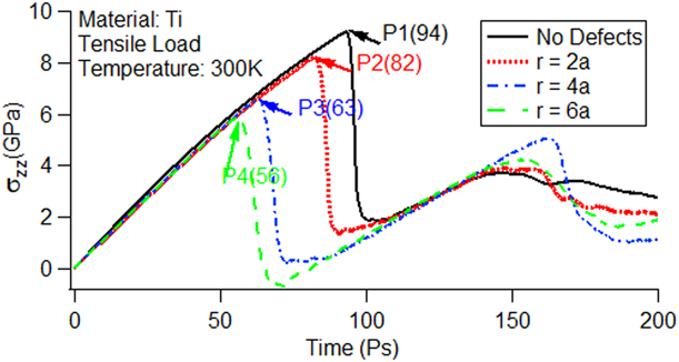
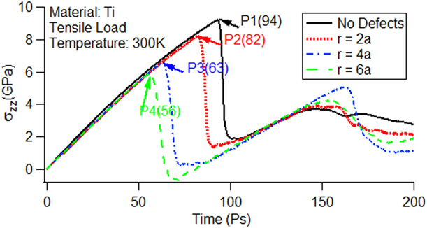
The stress–time curves with and without void defects under uniaxial stress conditions are shown in Fig. 1. From the figure, we can analyze the deformation process of single-crystal Ti during tension. When the material is in the elastic stage, its corresponding Young’s modulus is basically equal, but the peak value decreases with the increase in void size, which is similar to the previously reported results [Reference Yang, Zhang and Zhao23]. We used P1 to represent peak with no defects and P2, P3, and P4 to represent peaks with void sizes with radii of r = 2a, r = 4a, and r = 6a, respectively. The numbers in parentheses stand for the corresponding time in picoseconds. Rawat and Mitra explained the reason for the appearance of peaks in an investigation of the c-axis compression of single-crystal Ti under uniaxial stress conditions [Reference Rawat and Mitra10].
Axial stress–time curves for single-crystal titanium using the Henning potential.
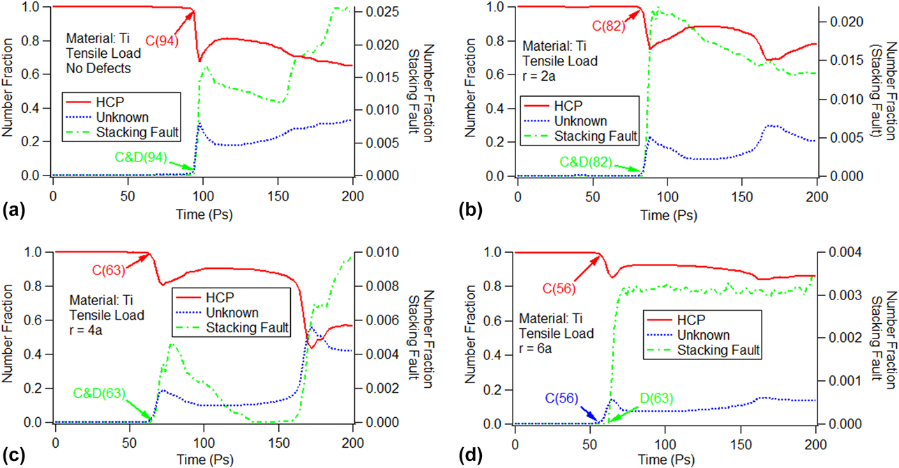
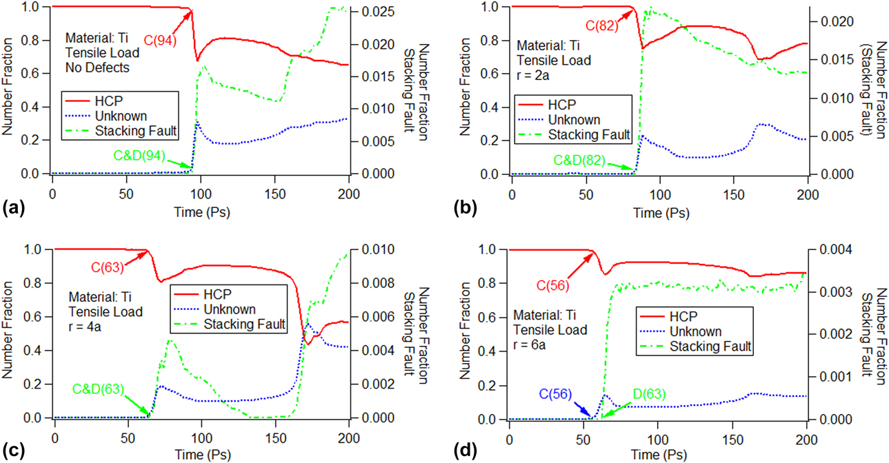
To verify the cause of the peaks in Fig. 1, we used the crystal analysis tool (CAT). The number fraction of the HCP structure (atoms are part of the parent HCP structure), stacking fault (atoms are part of the stacking fault), and unknown structure (atoms with an unknown coordination number) versus time is shown in Fig. 2. In the figure, the vertical axis on the left side is for the number fraction of the HCP and unknown structures, whereas that on the right side is for the number fraction of the stacking fault. The figure shows that the number fraction of the HCP structure is approximately 100%, whereas that for the unknown structures and the stacking fault is small for the cases with no defects and other void sizes at the beginning. We use “C” to mark the break points for the number fraction decrease of the HCP structure as well as the appearance for the unknown structures, and use “D” to mark the creation of the stacking fault in the figure. In addition to the marks, the corresponding times are enclosed in parentheses. It is obvious that for the cases with no defects [Fig. 2(a)] and with void sizes of r = 2a [Fig. 2(b)] and r = 4a [Fig. 2(c)], the corresponding times for the break points marked with “C” and “D” are the same as those for the P1, P2, and P3 points in the stress–time curves shown in Fig. 1. For the void size of r = 6a, the number fraction decrease of the HCP structure and the appearance of the unknown structure occur at the same time, i.e., 56 ps as shown in Fig. 2(d). The time is identical to that at the P4 peak in the stress–time curves (see Fig. 1). However, the stacking fault is created at 63 ps, which is marked as “D” in Fig. 2(d), and is later than the appearance of the HCP or unknown structure. We can conclude that the peaks in the stress–time curves could be due to the appearance of the unknown structure.
Time evolution of the atomic number fraction for the HCP structure, stacking fault, and unknown structure without voids and with different void sizes: (a) no defects, (b) r = 2a, (c) r = 4a, and (d) r = 6a.
Twin analysis
The peaks in the stress–time curves in Fig. 1 could be due to lattice rotation. The simulation of single-crystal Ti under uniaxial stress conditions reveals that some HCP atom clusters have different orientations compared with the parent HCP atom clusters, which indicates the activation of tension twins. To identify this, we performed a c-axis misorientation analysis, indicating the activation of the  $\left\{ {10\bar{1}2} \right\}$ twin system [Reference Rawat and Mitra24]. Table I shows the Schmid factors for all six variants (three conjugate variant pairs) calculated for the loading directions [Reference Bao, Schuman, Lecomte, Philippe, Zhao and Esling25, Reference Godet, Jiang, Luo and Jonas26]. To distinguish the variants from each other, the twin variants are labeled as V1, V2, V3, V4, V5, and V6. According to the Schmid criterion, the larger the Schmid factor of the twin system, the easier it is to activate.
Schmid factor and misorientation angle for the tension twin systems.

For the  $\left\{ {10\bar{1}2} \right\}$ twin systems, the activation of all twin variants meets the Schmid criterion in the perfect single-crystal Ti. In contrast, whether the activation of the
 $\left\{ {10\bar{1}2} \right\}$ twin variants meet the Schmid criterion for the defective single-crystal Ti needs further verification.
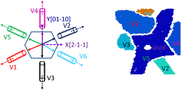
The snapshots of the activated twin variants of the  $\left\{ {10\bar{1}2} \right\}$ twin system with a void size of radius r = 2a at 82 ps are shown in Fig. 3. There are six twin variants for the
 $\left\{ {10\bar{1}2} \right\}$ twin system, which are represented in different colors.
Snapshots of the activated twin variants of the  $\left\{ {10\bar{1}2} \right\}$ twin system (r = 2a) (82 ps).
The time evolution of the total twin volume fraction and twin variant volume fraction for the  $\left\{ {10\bar{1}2} \right\}$ twin system is shown in Fig. 4. The vertical axis in the figure is the twin volume fraction (atoms are part of different twin variants). Whether or not the model contained voids, the total twin volume fraction first appears to increase rapidly as a result of the rapid growth of the twins. Thereafter, it increases slowly as a result of the interaction between twins belonging to other variants, which obstructs the growth of the twins. For the model without void defects [Fig. 4(a)], all twin variants of the
 $\left\{ {10\bar{1}2} \right\}$ twin system appear simultaneously and continue to increase slowly. As the stretching process proceeds, all twin variants remain; however, each twin variant has a different volume fraction, although they have the same Schmid factor. This indicates that the evolution and dominance of the twin variants do not meet the Schmid criterion.
Time evolution of the total twin volume fraction and twin variant volume fraction for the  $\left\{ {10\bar{1}2} \right\}$ twin system: (a) no defects, (b) r = 2a, (c) r = 4a, and (d) r = 6a.
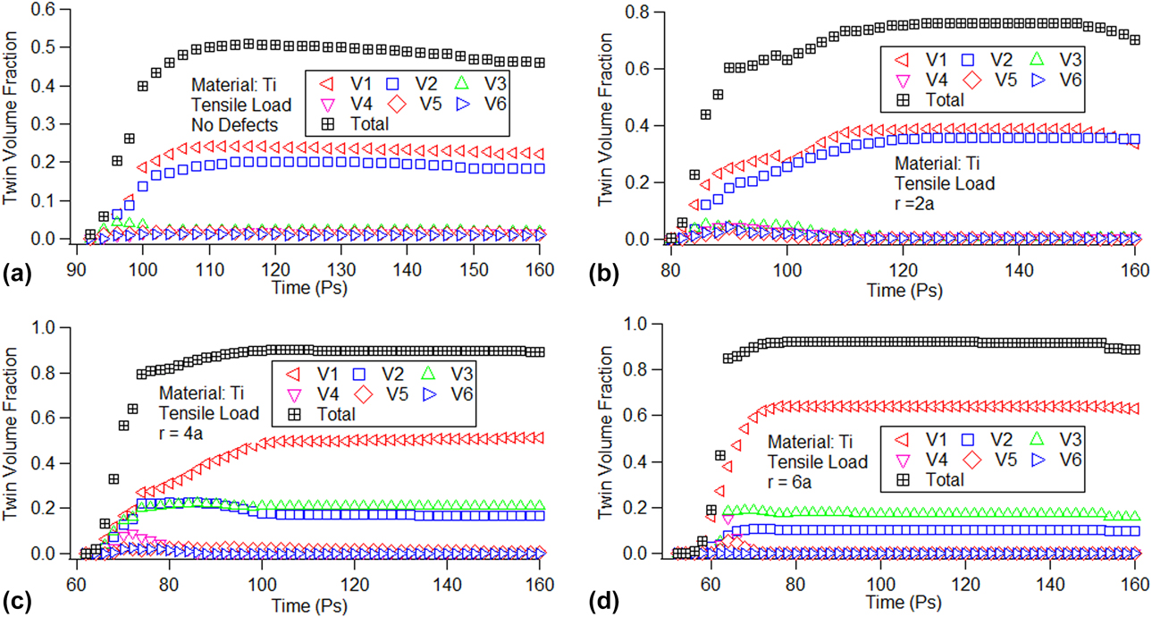
To further explore the effect of void sizes on the dominance of the V1, V2, and V3 twin variants, we analyzed the relationship between void sizes and these three twin variants. Figure 4 shows that all the twin variants begin to decrease after 150 ps. We chose this time point for analysis, and the volume fractions of the V1, V2 and, V3 twin variants at 150 ps are shown in S1 (see Supplementary material S1). Because the volume fractions of the V4, V5, and V6 twin variants are too small, we do not discuss them further here. S1 shows that the volume fraction of the V1 twin variant increases almost linearly, whereas those of the V2 and V3 twin variants increase once and then decrease with the increase in void size. This indicates that the void sizes affect the spatial distribution of nucleated twins belonging to different variants. The exact reasons need to be further studied.
Dislocation analysis
The formal results indicate that the microstructure evolution of the model with existing voids is quite different from that of the perfect model. To understand the activation of the slip systems and the microstructure evolution, we performed a dislocation analysis using the dislocation extraction algorithm (DXA) implemented in OVITO. The DXA separates the crystal into good and bad crystal regions using the common neighbor analysis method [Reference Honeycutt and Andersen27]. To obtain the dislocation information, the algorithm uses the Delaunay tessellation, wherein the tessellation edges (which define a set of elementary atom-to-atom steps) are used to construct the Burgers circuit. As it is not possible to construct all possible Burgers circuits to find the dislocation in a crystal, the algorithm extracts the information for a boundary surface separating the good and the bad regions. This boundary, known as the interface mesh, includes those triangular Delaunay facets, which have a good tetrahedral element on one side and a bad element on the other side. Once the interface meshes are identified, the algorithm constructs all possible Burgers circuits on the interface meshes to find all dislocations [Reference Lubarda, Schneider, Kalantar, Remington and Meyers28].
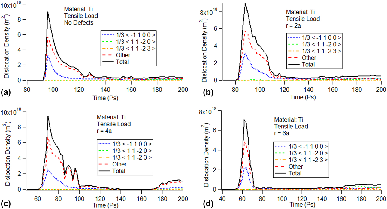
The evolution of the dislocation density versus time with and without a void size is shown in Fig. 5. The vertical axis in the figure is the dislocation density of the system. Analysis of the Burgers vector shows that there are three types of dislocation present in the system: (i)  ${1 \over 3}\left\langle {\bar{1}100} \right\rangle$ partial dislocations on the basal plane, (ii)
 ${1 \over 3}\left\langle {11\bar{2}0} \right\rangle$ prismatic dislocations, and (iii)
 ${1 \over 3}\left\langle {11\bar{2}3} \right\rangle$ pyramidal dislocations. Some other dislocations could not be identified by the DXA.
Evolution of the dislocation density determined using the Henning potential: (a) no defects, (b) r = 2a, (c) r = 4a, and (d) r = 6a.
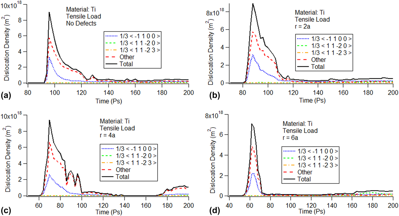
In Fig. 5, the trend of the dislocation density is similar regardless of whether the model contains void defects. In Fig. 5(b), for example, all dislocations increase rapidly at the beginning and then all the dislocation densities reached the maximum almost simultaneously before rapidly dropping to the minimum. The  ${1 \over 3}\left\langle {\bar{1}100} \right\rangle$ partial dislocation density and other dislocation densities are dominant in the total dislocation density. In contrast, the
 ${1 \over 3}\left\langle {11\bar{2}0} \right\rangle$ prismatic dislocation density and the
 ${1 \over 3}\left\langle {11\bar{2}3} \right\rangle$ pyramidal dislocation density have less of an impact on the total dislocation density. For the cases with no defect [Fig. 5(a)] and with void sizes of r = 2a [Fig. 5(b)], r = 4a [Fig. 5(c)], and r = 6a [Fig. 5(d)], the trend of the dislocation density is the same; however, the maximum value of the
 ${1 \over 3}\left\langle {\bar{1}100} \right\rangle$ partial dislocation density decreases with the increase in void size. Comparing Figs. 5 with 4, the dislocations appear at basically the same the time as the activation of the twin variants, which indicates the possible correlation between the two.
For the  ${1 \over 3}\left\langle {\bar{1}100} \right\rangle$ partial dislocation, the maximum value of the
 ${1 \over 3}\left\langle {\bar{1}100} \right\rangle$ partial dislocation density for the model without and with different void sizes is shown in S2 (see Supplementary material S2). The peak value of dislocation density of the
 ${1 \over 3}\left\langle {\bar{1}100} \right\rangle$ partial dislocation decreases with the increase in void size, which indicates that void size has an impact on the emission and movement of dislocation loops.
Microstructure analysis
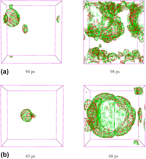
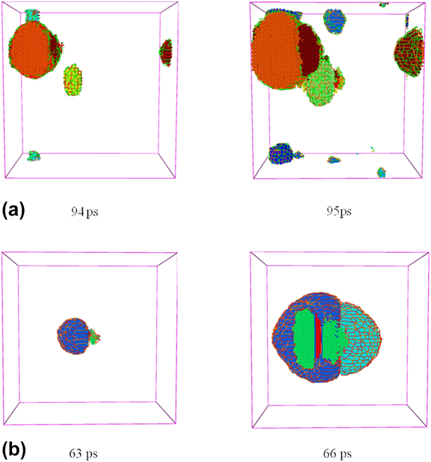
To better explore the correlation between twin volume fraction and dislocation density, we performed a microstructure analysis for the single-crystal Ti model. We chose two cases: one without void defects and the other with void defects. The snapshots of the microstructure changes at different time are shown in Fig. 6. We chose the time point corresponding to the first stress drop in the stress–time curve. The different colors represent the different dislocation networks ( ${1 \over 3}\left\langle {\bar{1}100} \right\rangle$ partial dislocations are in red, other dislocations are in green,
 ${1 \over 3}\left\langle {11\bar{2}0} \right\rangle$ prismatic dislocations are in violet, and
 ${1 \over 3}\left\langle {11\bar{2}3} \right\rangle$ pyramidal dislocations are in yellow). For the model without defects, shown in Figs. 6(a) and 6(b), we observe the evolution of the dislocation density during the tension processes, the emission of dislocation loops starts from the sides, and the number of dislocation loops increases as the tension progresses. However, when there is a void in the model, the emission of dislocation loops starts from the void [Reference Lubarda, Schneider, Kalantar, Remington and Meyers28, Reference Ohashi29, Reference Traiviratana, Bringa, Benson and Meyers30]; thereafter, it gradually starts from the sides.
Snapshots of the evolution of the dislocation densities: (a) no defects and (b) r = 4a.
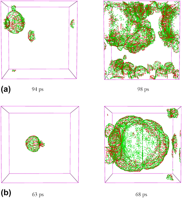
Figure 6 shows that the red ( ${1 \over 3}\left\langle {\bar{1}100} \right\rangle$ partial dislocations) and green (other dislocations) dislocation networks are dominant in the super cell, which indicates that the dislocation density is relatively high. This result is consistent with the previous dislocation density curves, as shown in Fig. 5.
Next, we analyzed the activation of the twin variants. When the model does not contain voids, the twin variants are first activated around the sides, whereas when it contains a void, the twin variants are first activated around the void. The activation process of the twin variants is very similar to that of the emission of dislocation loops, which indicates that the two processes are intrinsically linked. The snapshots of the microstructural evolution of twin variants and emission of dislocation loops, as observed in OVITO, show that twin variants increase with the movement of dislocation loops (Fig. 7).
Snapshots of microstructural evolution of twin variants and the emission of the dislocation loops: (a) no defects and (b) r = 4a.
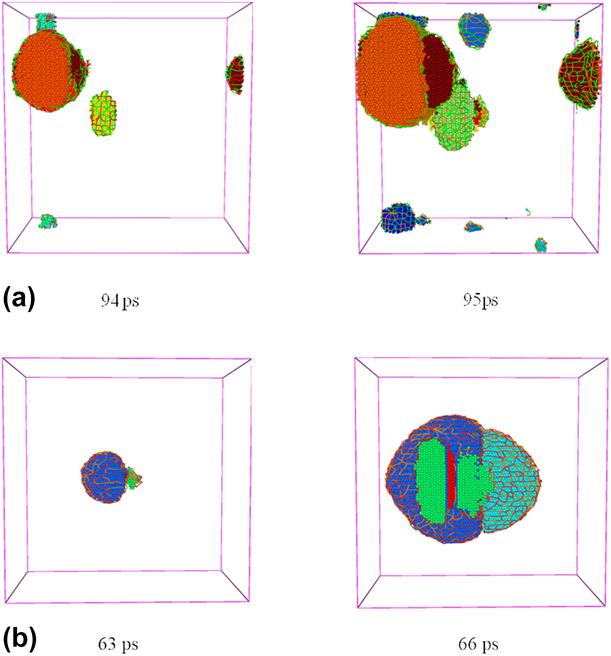
Cottrell and Bilby proposed that twin formation occurs through the polar axis mechanism of dislocation multiplication [Reference Cottrell and Bilby31, Reference Cottrell and Bilby32]. Through the movement of Shockley partial dislocations, the swept atomic layer keeps twinning. Therefore, the existence of a void is conducive to the emission of partial dislocation loops, which, in turn, is conducive to the activation and growth of twin variants. Figure 7 shows different colored atom clusters representing different twin variants. A layer of dislocation networks surrounds the cluster. As the tension proceeds, dislocation networks continue to expand to the model sides and twin variants continue to grow simultaneously with the movements of the dislocation network at the same time. The volume fraction varies for different clusters, which indicates that the evolution and dominance of the  $\left\{ {10\bar{1}2} \right\}$ twin variants do not follow the Schmid criterion even with the same Schmid factor. This phenomenon reveals whether the model contains defects, as the evolution and dominance of the
 $\left\{ {10\bar{1}2} \right\}$ twin variants do not follow the Schmid criterion in the tension process of single-crystal Ti.
Summary and conclusions
In this study, we simulated the c-axis tension of single-crystal Ti under uniaxial stress conditions without void defects and with different initial void sizes using the Henning potential. We also analyzed the tension twins and dislocations.
We found that the void defect has a significant effect on the plastic deformation of single-crystal Ti. We also found that single-crystal Ti with void defects does not meet the Schmid factor in the activation and evolution of twin variants. The existence of void defects affects not only the emission but also the movement of dislocation loops. The main conclusions are as follows:
(1) The activated twin variants do not contribute equally to the total twin volume with the same Schmid factor. The phenomenon becomes even more obvious with the increase in void size, which indicates that the Schmid factor does not effectively predict the evolution and dominance of the twin variants.
(2) The peak value of stress–strain curve decreases due to the generation of unknown structures, and the existence of void defects is beneficial to the generation of unknown structures.
(3) Without void defects, the emission of dislocation loops begins at the sides; in contrast, with void defects, it starts from the void. The existence of void defects exactly influences the density of the dislocation loops, and the void changes the nucleation site or the emission site of the variants and loops.
(4) The existence of voids hinders the movement of dislocation loops. With the increase in void sizes, the peak value of the
 ${1 \over 3}\left\langle {\bar{1}100} \right\rangle$ partial dislocation density decreases continuously.

Computational method
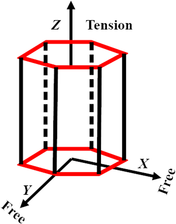
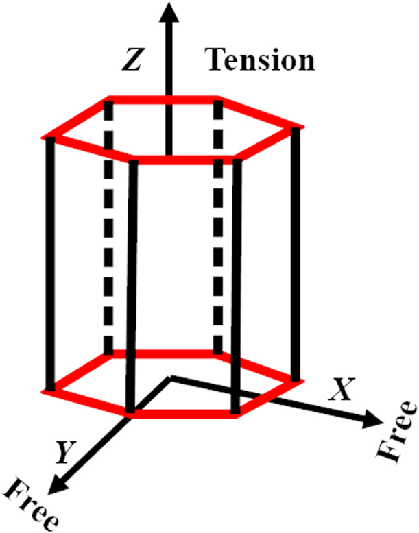
In this work, we simulated the c-axis tension of single-crystal Ti at room temperature under uniaxial stress conditions using the Henning potential [Reference Hennig, Lenosky, Trinkle, Rudin and Wilkins33]. A representative diagram of the uniaxial stress and strain conditions is shown in Fig. 8. For the uniaxial stress conditions, the pressure of X- and Y-directions is kept at 0 bar, thereby allowing the material to change size and shape along these directions.
c-axis tension under uniaxial stress conditions.
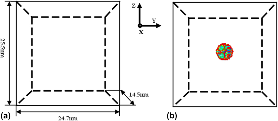
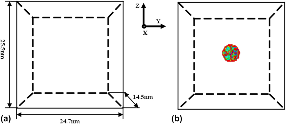
We used Large-scale Atomic/Molecular Massively Parallel Simulator (LAMMPS) [Reference Plimpton34] to simulate single-crystal Ti subjected to axial tension under uniaxial stress conditions (σxx = 0, σyy = 0, σzz ≠ 0). The size of the model is 14.5 nm × 24.7 nm × 25.5 nm and it contains 5 × 10⁵ atoms. The X-, Y-, and Z-directions of the simulation correspond to  $\left\langle {2\bar{1}10} \right\rangle$,
 $\left\langle {01\bar{1}0} \right\rangle$, and 〈0001〉, respectively. We adopted the periodic boundary conditions in the model and chose the velocity Verlet algorithm to integrate the equation of motion with a time step of 2 fs [Reference Martys and Mountain35]. We selected a spline-based modified embedded atom method potential called the Henning potential [Reference Hennig, Lenosky, Trinkle, Rudin and Wilkins33]. We adopted the Nose–Hoover thermostat and barostat to control the temperature and pressure [Reference Evans and Holian36]. When the system was at initial equilibrium state, the temperature and pressure were set to 300 K and 0 bar, respectively. The total relaxation time was 40 ps, and then a strain rate of 1 × 10⁹ s−1 was applied along the Z-axis (c-axis) to stretch the system at a constant temperature of 300 K; meanwhile, the pressure along the X- and Y directions was kept at 0 bar by applying an NPT ensemble.
Void defects in single crystals have a great influence on its properties. The existence of void defects has an effect on twinning and dislocation evolution in single-crystal plastic deformation. In this paper, we will consider adding void defects in single-crystal titanium. The voids are spherical, and their radii are 2a, 4a, and 6a (where a is a lattice constant, which is equal to 2.95 Å). Figure 9 shows a schematic diagram of the models without and with void defects (r = 6a). The different colors for atoms in Fig. 9(b) indicate the distance between atoms that is determined with common neighbor analysis [Reference Honeycutt and Andersen27]. Then, using a basal plane [Reference Barrett, Tschopp and El Kadiri11] and a CAT [Reference Stukowski, Bulatov and Arsenlis37], we performed a post-processing of the atomic data. The results were visualized in OVITO [Reference Stukowski38].
Schematic diagram of the models: (a) no defects; (b) r = 6a.
Supplementary material
To view supplementary material for this article, please visit https://doi.org/10.1557/jmr.2019.279.
Acknowledgments
The authors would like to deeply appreciate the support from the National Natural Sciences Foundation of China (11572191, 51701117, and 51779139) and the Shanghai Science and Technology Committee Foundation (17411962200).