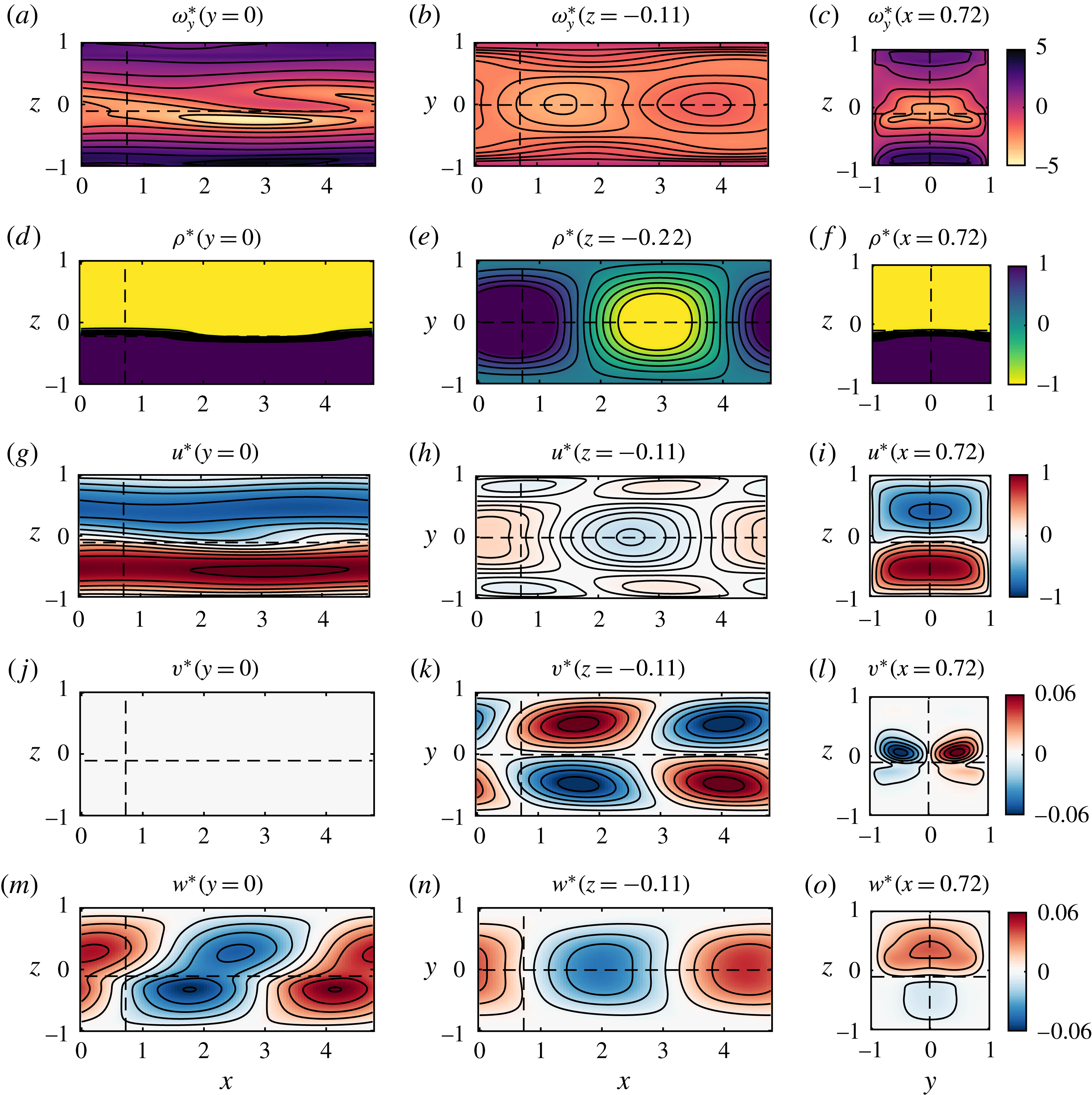
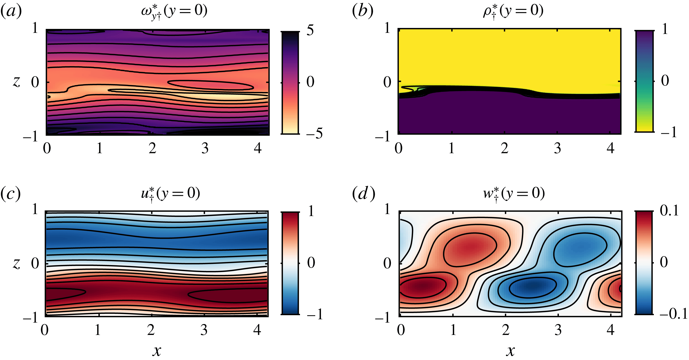
1 Introduction
The onset of instabilities triggering the transition to turbulence and consequent irreversible mixing in stratified shear flows is a fundamental problem in fluid mechanics, and was first recognised as such by Osborne Reynolds who observed instabilities on an interface between two immiscible fluids. In his classic paper, usually cited for his pipe flow experiments, Reynolds (Reference Reynolds1883) established a shear flow in a two-layer fluid by tilting a closed tube. He noted it was ‘a very pretty experiment’ which showed that ‘there is a critical velocity…at which direct motion becomes unstable’ and that ‘the instability…did not depend on the magnitude of the disturbances’. The first application of linear stability theory to stratified shear flows was described by G. I. Taylor in his Adams Prize essay of 1915 entitled ‘Turbulent motion in fluids’. Though Taylor published his stability predictions ‘without waiting for experimental results’ (Taylor Reference Taylor1931), the influential and beautiful ‘tilting tank’ experiments by Thorpe (Reference Thorpe1971) demonstrated that the development and turbulent break down of classical linear instabilities of stratified shear flows can be observed and measured in the laboratory.
Since the pioneering work of Woods (Reference Woods1968), observational evidence has also accumulated that finite-amplitude manifestations of stratified shear flow instabilities occur frequently in the oceans and atmosphere (see e.g. van Haren et al. Reference van Haren, Gostiaux, Morozov and Tarakanov2014, Mahrt Reference Mahrt2014). The mixing induced by the turbulence following these instabilities is thought to play a key role in diapycnal transport (see Ivey, Winters & Koseff Reference Ivey, Winters and Koseff2008 for a review). Since turbulent mixing occurs on small scales relative to the current resolution of general circulation and climate models, the development of subgrid-scale parameterisations to model diapycnal mixing remains essential. However, there is still uncertainty concerning the causal relationship between bulk flow properties, spatio-temporally intermittent turbulence and irreversible mixing.
A promising avenue of research to address this uncertainty is to analyse stratified turbulence in a dynamical systems framework, focusing on spatio-temporal structures rather than statistics. Within this approach, an interesting hypothesis is that the dynamics of turbulence can be described as an, in general complicated, trajectory in phase space that spends significant periods in the vicinity of a set of unstable nonlinear exact solutions of the Navier–Stokes equations called ‘exact coherent states’ (see e.g. Gibson, Halcrow & Cvitanović Reference Gibson, Halcrow and Cvitanović2008). In certain circumstances, these exact coherent states can be traced back, generically through a sequence of bifurcations, to linear instabilities (Lucas, Caulfield & Kerswell Reference Lucas, Caulfield and Kerswell2017). They can also provide useful insights into the properties of the turbulent attractor, for example by allowing for reduced-order modelling of key quantities such as energy dissipation (Lucas & Kerswell Reference Lucas and Kerswell2015) and irreversible mixing in stratified flows (Lucas & Caulfield Reference Lucas and Caulfield2017). It is, however, proving extremely challenging to identify such exact coherent states in numerical simulations of flows prone to vigorous turbulence. This issue is particularly significant in stratified flows relevant to the ocean due to the large values of the Prandtl number
 $Pr\equiv \unicode[STIX]{x1D708}/\unicode[STIX]{x1D705}\approx 7$
and Schmidt number
 $Sc\equiv \unicode[STIX]{x1D708}/\unicode[STIX]{x1D705}_{s}\approx 700$
, where
 $\unicode[STIX]{x1D708}$
is the kinematic viscosity,
 $\unicode[STIX]{x1D705}$
is the thermal diffusivity and
 $\unicode[STIX]{x1D705}_{s}$
is the salt diffusivity. The tendency of those flows to develop well-mixed layers separated by sharp density gradients (at least intermittently; see Salehipour, Caulfield & Peltier Reference Salehipour, Caulfield and Peltier2016), makes their direct numerical simulation beyond current computational capabilities. Therefore, laboratory experiments have an important role to play in guiding theoretical and numerical work towards the identification of dynamically important exact coherent states, under the hypothesis that they leave a distinctive signature in experimental turbulent flow, as observable, inherently nonlinear, yet relatively long-lived coherent structures.
In this paper, we describe an apparently previously unidentified coherent structure in a sustained laboratory stratified shear flow. The stratified inclined duct experiment, described by Meyer & Linden (Reference Meyer and Linden2014), generates a two-layer stratified exchange flow in an inclined duct connecting two reservoirs containing fluids of different densities. As discussed in more detail by Meyer & Linden (Reference Meyer and Linden2014), variations in the density difference and/or inclination angle (a few degrees at most) lead to four qualitatively different observed flow states:
(i) laminar flow, characterised by a thin, flat density interface;
(ii) a largely coherent, but non-parallel flow state characterised by robust, propagating, quasi-periodic waves on the interface;
(iii) spatio-temporally intermittent turbulence with small-scale structures and mixing;
(iv) fully developed turbulence with significant small-scale structures and a thick mixed interfacial density layer.
Here we focus on the coherent wave state (ii), which Meyer & Linden (Reference Meyer and Linden2014) described as the ‘Holmboe regime’, since the waves observed using a shadowgraph were very similar in appearance to the finite-amplitude manifestation of the instability predicted by Holmboe (Reference Holmboe1962), observed experimentally by Thorpe (Reference Thorpe1968) in tilting tank experiments, and numerically simulated (in two-dimensional flows) first by Smyth, Klaassen & Peltier (Reference Smyth, Klaassen and Peltier1988). As we shall see, the coherent structure that we observe has close connections to the finite-amplitude waves arising from the traditional (two-dimensional) Holmboe instability, but exhibits three-dimensionality and spanwise confinement within our experimental duct. Therefore, we refer to this structure as a ‘confined Holmboe wave’ (CHW). The aim of this paper is to characterise this structure, and to understand how it originates, in the specific sense of identifying and understanding the underlying physical mechanisms that lead to the observed behaviour.
We characterise the three-dimensional structure of the CHW using a novel technique allowing time-resolved near-instantaneous measurements of all three velocity components and density field over a three-dimensional volume. We demonstrate that many aspects of the observed CHW are consistent with the predictions of a linear normal mode stability analysis of the experimentally measured, quasi-steady background flow which develops within the duct. We call this instability the ‘confined Holmboe instability’ (CHI). Note that, in the rest of the paper, we aim to distinguish in general between
(i) an infinitesimally small perturbation that is linearly unstable, which we typically refer to as an instability;
(ii) a finite-amplitude, nonlinear wave, which we typically refer to as a wave.
To address our above-mentioned aim of characterising and identifying the physical mechanisms at the origin of the CHW observed in the stratified inclined duct, the remainder of this paper is organised as follows. In § 2 we review relevant previous work, particularly on the traditional, two-dimensional Holmboe instability, to contextualise and motivate our study. In § 3 we describe the experiment and measurement technique, and present the experimental results to characterise the CHW in § 4. In § 5 we describe our linear stability analyses and compare their predictions (including the CHI) with our experimental data in § 6. Finally we present our conclusions, and suggest possible future research directions in § 7.
2 Context and motivation
2.1 Holmboe instabilities
Holmboe (Reference Holmboe1962) considered the stability of an idealised two-layer stratification embedded within a shear layer of finite depth, and demonstrated that, for sufficiently strong stratification, such inviscid flows are always linearly unstable over a finite band of wavenumbers. He considered a symmetric configuration, with the density interface located at the mid-point of the shear layer, so there are two normal modes (with equal and opposite phase speeds) with equal growth rates in this instability band of wavenumbers.
This instability, which we refer to as the ‘traditional’ Holmboe instability, can be interpreted physically as being due to a resonance between infinitesimal internal wave-like perturbations localised at the density interface and infinitesimal Rayleigh (or ‘vorticity’) wave-like perturbations localised at the edges of the shear layers (Baines & Mitsudera Reference Baines and Mitsudera1994; Caulfield Reference Caulfield1994). This interpretation is a particular example of the ‘wave interaction theory’ for the identification and classification of instabilities (see Carpenter et al. (Reference Carpenter, Tedford, Heifetz and Lawrence2013) for a review). The symmetric problem considered by Holmboe (Reference Holmboe1962) has two such resonances simultaneously, leading to two instabilities: one localised in the upper half of the shear layer, the other in the lower half of the shear layer. However, this physical internal wave–vorticity wave interaction instability mechanism is generic and gives rise to instabilities sharing the same essential features as the traditional Holmboe instability in more general stratified shear flows with finite depth shear layers with embedded ‘sharp’ density interfaces. It is this generic class of instabilities that we, for simplicity, refer to as Holmboe instabilities (HIs).
Lawrence, Browand & Redekopp (Reference Lawrence, Browand and Redekopp1991) generalised the original stability calculations of Holmboe to consider asymmetric flows where the sharp density interface and the mid-point of the shear layer are not coincident. This breaks the symmetry of the traditional stability problem, giving rise to two instabilities with different growth rates, phase speeds and wavenumber bands for a given stratification. For flows in domains that are not bounded vertically, the resonance between the infinitesimal internal wave-like perturbation localised at the density interface and the vorticity wave-like perturbation localised at the further edge of shear layer gives rise to the assumed dominant instability band, with larger maximum predicted growth rate, smaller magnitude phase speed and smaller wavenumbers. Haigh & Lawrence (Reference Haigh and Lawrence1999) further demonstrated that vertical confinement by sufficiently close top and bottom boundaries could switch the dominant branch of instability, consistent with the seminal work of Hazel (Reference Hazel1972).
2.2 Holmboe waves: laboratory observations and numerical simulations
Finite-amplitude manifestations of HIs, which we refer to as Holmboe waves (HWs), have been observed experimentally in a wide range of shear flows containing relatively sharp density interfaces (see e.g. Macagno & Rouse Reference Macagno and Rouse1961; Thorpe Reference Thorpe1968; Browand & Winant Reference Browand and Winant1973; Maxworthy & Browand Reference Maxworthy and Browand1975; Caulfield et al. Reference Caulfield, Peltier, Yoshida and Ohtani1995; Zhu & Lawrence Reference Zhu and Lawrence2001; Hogg & Ivey Reference Hogg and Ivey2003; Tedford, Pieters & Lawrence Reference Tedford, Pieters and Lawrence2009; Carpenter et al. Reference Carpenter, Tedford, Rahmani and Lawrence2010; Meyer & Linden Reference Meyer and Linden2014). Generically, cusped waves are observed at the interface, propagating at a phase speed intermediate between the propagation speed of the density interface and the maximum speed of the sheared fluid, in qualitative agreement with linear stability theory.
Zhu & Lawrence (Reference Zhu and Lawrence2001) observed both symmetric (up–down) and asymmetric (only up or only down) HWs in a laboratory exchange flow. They compared their observations with two different normal mode stability calculations. One calculation used the piecewise-linear profiles originally considered by Holmboe (Reference Holmboe1962), while the other used smooth parallel velocity and density profiles, calculated as solutions to the Taylor–Goldstein equation by Nishida & Yoshida (Reference Nishida and Yoshida1990). They found only qualitative agreement with the predicted phase speeds and wavelengths, perhaps unsurprisingly due to the highly idealised nature of the assumed velocity and density profiles compared to the actual laboratory flows. Tedford et al. (Reference Tedford, Pieters and Lawrence2009) and Carpenter et al. (Reference Carpenter, Tedford, Rahmani and Lawrence2010) conducted further experiments, and the latter made the first comparison with three-dimensional direct numerical simulations (DNS). They attributed the discrepancy between experiments and linear theory to wave stretching (increasing wavelength by the streamwise convective acceleration of the mean flow), and the discrepancy between DNS and linear theory to wave merging (increasing wavelength by vortex merging events). They also found that the wave amplitude was larger in the DNS than in the experiments, although the simulations did not correspond exactly to the experimental situation, in particular in the choice of the Schmidt number.
In the first two-dimensional DNS of HWs, Smyth et al. (Reference Smyth, Klaassen and Peltier1988) established that the counter-propagating trains of HWs above and below the (symmetrically located) density interface accelerate when the crests of the characteristic cusped waves are aligned vertically, and slow down when they are laterally far apart. As is apparent in their figure 7, this behaviour is associated with the relative location of the elliptical spanwise vortices that develop in front of the density crests, with the slowing occurring when the two vortices are close to being aligned vertically (corresponding to density crests being far apart). Indeed, for sufficiently weak stratification, these two vortices ‘lock’ and then roll up the interface into an array or ‘train’ of elliptical billows, i.e. the finite-amplitude manifestation of the Rayleigh instability of a finite-depth shear layer (see Rayleigh Reference Rayleigh1879, and for further discussion of this phenomenon for ‘marginal’ HWs, Smyth & Peltier Reference Smyth and Peltier1991). Such structures are commonly referred to as ‘Kelvin–Helmholtz billows’, even though Kelvin (Thomson Reference Thomson1871) and Helmholtz (Reference Helmholtz1878) only considered a discontinuous velocity profile, which does not exhibit the scale selection characteristic of billow trains.
The elliptical vortices of HWs develop close to the critical layers of the linear instability (i.e. where the predicted phase speed of the linear instability matches the flow speed). Due to the relatively strong baroclinic vorticity generation associated with the cusped waves, these vortices do not typically correspond to the maximum vorticity magnitude within the flow, although they typically induce the entrainment of ‘wisps’ of fluid from the crest of the propagating cusped waves.
Smyth & Peltier (Reference Smyth and Peltier1991) used secondary linear Floquet stability analysis, (i.e. the linear stability analysis of non-parallel flow fields extracted from two-dimensional numerical simulations under the assumption that these flow fields were ‘frozen’ in time) in an attempt to understand how a two-dimensional saturated HW becomes three-dimensional, breaks down and hence has the potential to undergo the transition to turbulence. Simulations at moderate Reynolds numbers suggested that HWs could be robust and identifiable over relatively long times (see for example Smyth & Winters Reference Smyth and Winters2003, Carpenter, Lawrence & Smyth Reference Carpenter, Lawrence and Smyth2007 and Smyth, Carpenter & Lawrence Reference Smyth, Carpenter and Lawrence2007). However, through simulations at significantly higher Reynolds number, Salehipour et al. (Reference Salehipour, Caulfield and Peltier2016) demonstrated that finite-amplitude symmetric HWs are prone to a wide range of secondary instabilities of both convective and shear-driven types, which destroy the coherence of the primary instability and trigger a relatively long period (at least in comparison to KH billow trains) of turbulent motions characterised by enhanced turbulent dissipation and irreversible mixing. Nevertheless, these behaviours at higher Reynolds numbers may well be inherently linked to the transient run-down nature of such simulations, with no forcing acting to re-energise the initial shear flow, and the initial profiles and computational domain geometry being chosen to be susceptible to specific (and typically monochromatic) linear instabilities.
2.3 Limitations of previous research
In this paper, we attempt to address some of the limitations of the previous studies of HWs, which we classify in three categories: steadiness; dissipation; and three-dimensionality.
2.3.1 Steadiness
To the best of our knowledge, all numerical calculations have considered the time evolution of an initially unstable state, analogous to the time-dependent instabilities observed in ‘tilting tank’ experiments of Reynolds (Reference Reynolds1883) and Thorpe (Reference Thorpe1971). This set-up is convenient for comparison with the predictions of linear stability theory in an initial value problem. However, many geophysically relevant flows – such as exchange flows in straits, estuaries (e.g. Geyer et al. Reference Geyer, Lavery, Scully and Trowbridge2010), coastal inlets (e.g. Farmer & Armi Reference Farmer and Armi1999), deep ocean overflows (e.g. van Haren et al. Reference van Haren, Gostiaux, Morozov and Tarakanov2014) and stratified flows in the atmospheric boundary layer (e.g. Mahrt Reference Mahrt2014) – are sustained in time through slowly varying forcing, such that a quasi-steady nonlinear state can exist. Such natural flows are not the product of carefully designed initial conditions chosen to trigger specific primary instabilities, which as noted above lead to inherently transient flow evolution and, in particular, preclude any possibility of finite-amplitude coherent structures emerging which are both robust and long-lived.
In contrast, the stratified inclined duct experiment sets up a statistically steady flow that is not the inevitable result of carefully designed initial conditions. HWs propagate throughout the duct and nonlinearly influence the mean flow that sustains them. This situation is more representative of environmental flows, yet there is no a priori rigorous argument justifying a connection between observed saturated nonlinear waves and linear instabilities predicted to grow from infinitesimal perturbations using the horizontally averaged mean flow as a notional, though not actually realised, base flow. In this paper we show that despite the undoubted challenge to this modelling approach, the comparison is, perhaps fortuitously, good.
2.3.2 Dissipation
The majority of the experiments and numerical calculations of which we are aware considered flows at relatively low Reynolds numbers of
 $O(10{-}100)$
(based on the definition (3.4) adopted later in this paper), with the recent exception of Salehipour et al. (Reference Salehipour, Caulfield and Peltier2016). Moreover, the ‘run-down’ character means that a strictly restricted amount of energy, set at the beginning of the flow evolution, is available to dissipate, and that this dissipation is inherently limited in time. Indeed, the stratified turbulence literature (see e.g. the review of Ivey et al. (Reference Ivey, Winters and Koseff2008)) increasingly highlights the importance of the ‘buoyancy Reynolds number’
 $Re_{b}$
, defined as
 $$\begin{eqnarray}\displaystyle Re_{b}\equiv \frac{\unicode[STIX]{x1D716}_{0}}{\unicode[STIX]{x1D708}N_{0}^{2}}. & & \displaystyle\end{eqnarray}$$
Here,
 $\unicode[STIX]{x1D716}_{0}$
is a characteristic (volume-averaged) value of the rate of dissipation of total kinetic energy
 $\unicode[STIX]{x1D716}\equiv 2\unicode[STIX]{x1D708}\unicode[STIX]{x1D634}_{ij}\unicode[STIX]{x1D634}_{ij}$
(where
 $\unicode[STIX]{x1D634}_{ij}\equiv (\unicode[STIX]{x2202}_{x_{i}}u_{j}+\unicode[STIX]{x2202}_{x_{j}}u_{i})/2$
is the symmetric strain rate tensor) and
 $N_{0}$
is a characteristic value of the buoyancy frequency
 $N\equiv \sqrt{-(g/\unicode[STIX]{x1D70C}_{0})\unicode[STIX]{x2202}_{z}\unicode[STIX]{x1D70C}}$
. This non-dimensional number, sometimes referred to as the ‘activity parameter’ or
 $Gn$
(Portwood et al.
Reference Portwood, de Bruyn Kops, Taylor, Salehipour and Caulfield2016), is the (square) ratio of the frequencies associated with kinetic energy dissipation
 $\sqrt{\unicode[STIX]{x1D716}/\unicode[STIX]{x1D708}}$
and buoyancy
 $N$
. An alternative and illuminating interpretation is to express
 $Re_{b}$
as a ratio of length scales:
 $Re_{b}=(L_{o}/L_{k})^{4/3}$
where
 $L_{o}=(\unicode[STIX]{x1D716}/N^{3})^{1/2}$
is the Ozmidov scale, the vertical scale below which turbulent eddies are not significantly affected by stratification, and
 $L_{k}=(\unicode[STIX]{x1D708}^{3}/\unicode[STIX]{x1D716})^{1/4}$
is the Kolmogorov scale, below which viscous dissipation dominates. The ratio
 $Re_{b}$
therefore measures the range of scales that are not significantly affected either by stratification (suppressing vertical scales
 ${\gtrsim}L_{o}$
) or by viscosity (damping scales
 ${\lesssim}10L_{k}$
). Although caution needs to be exercised when comparing different studies and flow geometries where
 $Re_{b}$
may be defined in different ways, consensus is developing, not least motivated by the arguments of Gibson (Reference Gibson and Nihoul1980) and Gibson (Reference Gibson1999), that
 $Re_{b}\gtrsim 20{-}30$
is required for the flow to exhibit any of the key characteristics of stratified turbulence (see Bartello & Tobias Reference Bartello and Tobias2013; Portwood et al.
Reference Portwood, de Bruyn Kops, Taylor, Salehipour and Caulfield2016 for further discussion).
In the stratified inclined duct experiment, we estimate the volume-averaged
 $Re_{b}\approx Re\sin \unicode[STIX]{x1D703}$
(see (3.4) and (3.6)) and CHWs are found to exist for
 $Re_{b}$
up to
 ${\approx}50$
, controlled by increasing either the Reynolds number
 $Re$
or the tilt angle of the duct
 $\unicode[STIX]{x1D703}$
(see § 3.4.1 for more details). We are therefore able to generate waves that maintain relatively high dissipation for hundreds of advective times units, making this experiment a viable attempt to reproduce inertia-dominated flows of geophysical relevance in the laboratory.
2.3.3 Three-dimensionality
Temporal linear stability analyses of parallel shear flows with a background streamwise velocity
 $U(z)\hat{\boldsymbol{x}}$
focus on wave-like disturbances, i.e. normal modes, of the form
 $$\begin{eqnarray}\displaystyle \unicode[STIX]{x1D6F9}^{\prime }(\boldsymbol{x}_{\bot },z,t)\equiv \hat{\unicode[STIX]{x1D6F9}}(z)\exp (\text{i}\boldsymbol{k}\boldsymbol{\cdot }\boldsymbol{x}_{\bot }+\unicode[STIX]{x1D70E}t), & & \displaystyle\end{eqnarray}$$
where
 $\hat{\unicode[STIX]{x1D6F9}}(z)$
is the one-dimensional complex eigenfunction of any perturbation variable;
 $z$
is the vertical coordinate;
 $\boldsymbol{x}_{\bot }\equiv x\hat{\boldsymbol{x}}+y\hat{\boldsymbol{y}}$
is the horizontal coordinate vector;
 $\boldsymbol{k}\equiv |\boldsymbol{k}|(\cos \unicode[STIX]{x1D6FD}\hat{\boldsymbol{x}}+\sin \unicode[STIX]{x1D6FD}\hat{\boldsymbol{y}})$
is the real horizontal wave vector; and
 $\unicode[STIX]{x1D70E}$
is the complex growth rate. Conventionally,
 $\boldsymbol{k}$
is taken to be aligned with the background flow along
 $x$
, i.e.
 $\unicode[STIX]{x1D6FD}=0$
. In this paper, we refer to such an analysis as ‘2P-1B’, for two-dimensional perturbations on a one-dimensional base flow and to the more general analysis with
 $\unicode[STIX]{x1D6FD}\neq 0$
as ‘2.5P-1B’, for its intermediate character between two- and three-dimensional perturbations. The focus on 2P-1B analyses can generically be justified by appealing to a corollary of ‘Squire’s theorem’ (Squire Reference Squire1933) in unstratified flows at finite Reynolds number, and the analogous ‘Yih’s theorem’ (Yih Reference Yih1955; Smyth et al.
Reference Smyth, Klaassen and Peltier1988) in (inviscid) stratified flow.
Both theorems rely on the observation that ‘three-dimensional’ normal modes aligned at some angle
 $\unicode[STIX]{x1D6FD}\neq 0$
to the background flow, having growth rate
 $\unicode[STIX]{x1D70E}$
, wavenumber
 $|\boldsymbol{k}|$
in a flow with Reynolds number
 $Re$
and bulk Richardson number
 $Ri$
are equivalent to ‘two-dimensional’ normal modes having
 $\unicode[STIX]{x1D6FD}=0$
with lower growth rate
 $(\unicode[STIX]{x1D70E}\cos \unicode[STIX]{x1D6FD})$
and larger wavenumber
 $(|\boldsymbol{k}|/\text{cos}\,\unicode[STIX]{x1D6FD})$
in an equivalent flow with lower Reynolds number
 $(Re\cos \unicode[STIX]{x1D6FD})$
and higher bulk Richardson number
 $(Ri/\text{cos}^{2}\,\unicode[STIX]{x1D6FD})$
. This statement is summarised by the relation (see Smyth & Peltier Reference Smyth and Peltier1990)
 $$\begin{eqnarray}\displaystyle \unicode[STIX]{x1D70E}(|\boldsymbol{k}|,\unicode[STIX]{x1D6FD},Re,Ri)=\cos \unicode[STIX]{x1D6FD}\;\unicode[STIX]{x1D70E}\left(\frac{|\boldsymbol{k}|}{\cos ~\unicode[STIX]{x1D6FD}},0,Re\cos \unicode[STIX]{x1D6FD},\frac{Ri}{\cos ^{2}\unicode[STIX]{x1D6FD}}\right). & & \displaystyle\end{eqnarray}$$
It is then natural to consider the locus of the two-dimensional modes (
 $\unicode[STIX]{x1D6FD}=0$
) with maximum growth rate
 $\unicode[STIX]{x1D70E}_{m}$
across all wavenumbers for given values of the external flow parameters
 $Re$
and
 $Ri$
. For an unstratified flow, if
 $\unicode[STIX]{x1D70E}_{m}(Re)$
decreases more slowly than
 $1/Re$
(i.e.
 $\unicode[STIX]{x1D70E}_{m}(Re)\times Re$
increases with
 $Re$
), then the most unstable two-dimensional modes have higher growth rates than any three-dimensional mode, a circumstance which is generic for shear flow instabilities. In particular, if instability occurs only above a critical Reynolds number (i.e. for
 $Re\geqslant Re_{c}$
), this condition implies that the marginal instability mode must be two-dimensional (as any three-dimensional mode in a flow with
 $Re=Re_{c}$
experiences an equivalent flow with
 $Re<Re_{c}$
, and hence is stable).
The equivalent statement for (inviscid) stratified flows is, if
 $\unicode[STIX]{x1D70E}_{m}(Ri)$
increases more slowly than
 $\sqrt{Ri}$
(i.e.
 $\unicode[STIX]{x1D70E}_{m}(Ri)/\sqrt{Ri}$
decreases with increasing
 $Ri$
), then the most unstable two-dimensional modes have higher growth rates than any three-dimensional mode. For stratified flows, the dominance of two-dimensional modes is not so clear cut, as HIs (for example) only occur in stratified flows, and occur for all bulk Richardson numbers, thus making it at least plausible that
 $\unicode[STIX]{x1D70E}_{m}(Ri)$
increases more rapidly than
 $\sqrt{Ri}$
. Indeed, in a stratified flow at finite Reynolds number, Smyth & Peltier (Reference Smyth and Peltier1990) identified a small parameter range in
 $Re{-}Ri$
space where
 $\unicode[STIX]{x1D70E}_{m}(Ri)$
does increase more rapidly than
 $\sqrt{Ri}$
and HIs at an angle
 $\unicode[STIX]{x1D6FD}\neq 0$
were predicted to be dominant, but it has proved difficult to test these predictions either experimentally or numerically.
It is important to recognise that such ‘three-dimensional’ modes considered by the 2.5P-1B analysis (in this precise sense of travelling at angle
 $\unicode[STIX]{x1D6FD}\neq 0$
to the background flow) are strictly only well defined in infinite domains with translational invariance in
 $x$
and
 $y$
. As another example of a ‘three-dimensional’ stability analysis, Drazin (Reference Drazin1974) considered the linear instability of an inviscid flow with two layers of different density, where the upper layer has a non-zero streamwise velocity which varies slowly in the spanwise direction. This flow is prone to a (truly) three-dimensional variant of the conventional Kelvin–Helmholtz instability, yet the background flow was still not confined or localised in any sense. Such flow instabilities, just like the flow instabilities ‘propagating at an angle’, are therefore unlikely to be observed experimentally. Furthermore, the modal structure (2.2) assumed for such perturbations inevitably imposes the same spanwise periodicity on the perturbation density and velocity components, thereby strongly restricting their possible spatial structure. As we discuss in more detail in this paper, perturbations with a more complex spatial structure are, in fact, consistent with our experimental observations.
Indeed, experimental observations of HWs are typically compared to HI ‘2P-1B’ predictions (often representing
 $U(z)$
by hyperbolic-tangent or error-function vertical profiles in unbounded domains). Analogously, three-dimensional numerical simulations typically consider periodic boundary conditions in both of the horizontal directions, avoiding potential issues with horizontal boundary conditions interacting with HWs. However, viscous effects and the presence of confining side walls in an experimental tank make any experimental mean flow inherently dependent on the spanwise (
 $y$
) and vertical (
 $z$
) coordinates and affect any waves which may develop by requiring the perturbations to decay to zero at these walls. Many of the geophysical flows mentioned in § 2.3.1 also exhibit two- or three-dimensional base flows and significant spatial confinement. It is therefore desirable to understand the effects of this inherent three-dimensionality and confinement and model them appropriately. Our experimental apparatus is designed to obtain data to achieve this.
3 The experiment
3.1 The stratified inclined duct
We consider the flow in a duct connecting two reservoirs containing aqueous salt solutions of densities
 $\unicode[STIX]{x1D70C}_{0}\pm \unicode[STIX]{x0394}\unicode[STIX]{x1D70C}/2$
(figure 1). The seal between the duct and the barrier separating the two reservoirs is made of flexible rubber, allowing the duct to tilt at a relatively small angle
 $\unicode[STIX]{x1D703}$
from the horizontal. The duct has length
 $L=1350$
mm and has a square cross-section of height and width
 $H=45$
mm (aspect ratio
 $L/H=30$
). At the start of the experiment, the duct is opened, initiating an exchange flow (with zero net volume flux) between the reservoirs.
Experimental flow geometry: an inclined duct (1) connects a reservoir of dense fluid (2) and a reservoir of light fluid (3). All fluid is seeded with particles for stereo particle image velocimetry (sPIV), and fluid initially in (3) is dyed for planar laser induced fluorescence (PLIF). The laser beam emitted from (4) is directed to the pair of oscillating mirrors in (5), before entering the light-sheet-producing optics mounted on the linear traverse (6). The scanning light sheet sweeps a measurement volume (7) whose successive planes are imaged for sPIV by cameras (8) and (9) and for PLIF by camera (10). The measurement volume inset shows the coordinate system and notation used, as discussed in § 3.2.

This flow is a two-layer stratified shear flow, forced by gravity in two distinct ways. The first contribution is a hydrostatic pressure gradient in each layer, resulting from the end of each duct sitting in reservoirs containing fluids of different densities, and is sufficient to drive an exchange flow at
 $\unicode[STIX]{x1D703}=0^{\circ }$
. The second contribution depends on the tilt angle: the resulting non-zero projection of gravity along the duct provides additional buoyancy forces. A positive angle
 $\unicode[STIX]{x1D703}>0^{\circ }$
(defined here by the duct being raised in the denser reservoir) reinforces the exchange flow by accelerating the light layer up (to the left) and the heavy layer down (to the right). Each individual reservoir measures
 $1\times 0.2\times 0.5$
m and holds approximately 100 l, allowing us to maintain a statistically steady exchange flow for several minutes. This steady flow continues until the controls at the ends of the duct (see below) are flooded by the accumulation of fluid of a different density coming from the other reservoir.
As outlined in § 1, Meyer & Linden (Reference Meyer and Linden2014) described and mapped four qualitatively different flow states obtained by varying the main parameters
 $\unicode[STIX]{x0394}\unicode[STIX]{x1D70C}/\unicode[STIX]{x1D70C}_{0}$
and
 $\unicode[STIX]{x1D703}$
, using shadowgraph observations and a larger square duct with length
 $L=3000$
mm and height
 $H=100$
mm. At low
 $\unicode[STIX]{x0394}\unicode[STIX]{x1D70C}/\unicode[STIX]{x1D70C}_{0}$
and
 $\unicode[STIX]{x1D703}$
, the flow is laminar with an undistorted interface. At larger values of either or both parameters, persistent coherent HWs distort the interface. Higher values of the forcing give rise to spatio-temporally intermittent turbulence at the interface, and eventually, fully developed turbulence with a thick mixing layer. Their measurements of layer-averaged velocities through mass flux balances support the hypothesis that the flow is hydraulically controlled at both ends of the duct for
 $\unicode[STIX]{x1D703}\gtrsim 1^{\circ }$
. The flow is subcritical (with respect to long, small-amplitude, interfacial disturbances) inside the duct, and undergoes two transitions at each end: a smooth one to a supercritical state shortly after exiting the duct, and an abrupt one further downstream (in the form of a jump) from supercritical to subcritical, to match the reservoir conditions. These hydraulic controls ensure that the exchange flow taking place through the duct is maximal, i.e. that its layer-averaged velocities obey the Froude number condition (3.1) (see Armi Reference Armi1986).
The practical consequence of this hydraulic control is that positive angles cannot increase the exchange flow rate, or mean flow velocities, beyond a certain value. The additional kinetic energy input provided by gravity through a positive tilt angle must be dissipated by the flow within the duct, either by increased wave activity or turbulence. We are therefore able to control the dissipation rate by the tilt angle, and to maintain target dissipation rates in a statistically steady sense for extended periods of time. The dissipation achieved is expressed non-dimensionally as a buoyancy Reynolds number in § 3.2, and depends on two free experimental parameters: the Reynolds number (when appropriately defined as in (3.4) and the tilt angle.
The inclined duct experiment is thus ideally suited to study HWs for the following reasons.
(i) It naturally sets up a flow with large shear layer thickness/density interface thickness ratio. The low diffusivity of salt compared to momentum (or high Schmidt number
 $Sc\approx 700$
, as defined in § 1), and the continuous supply of unmixed fluid from both reservoirs in the open duct mean that the interface thickness ratio resulting from interfacial diffusion of vorticity compared to interfacial diffusion of density is of the order of
$\sqrt{Sc}=O(10)$
.
(ii) It naturally sets up a flow with large bulk Richardson number. The hydraulic control sets an upper bound for the speeds achieved inside the duct and, as we shall see in § 3.2 and from (3.5), effectively sets the overall or bulk Richardson number to an
$O(0.1{-}1)$
constant, regardless of the forcing parameters.(iii) Both symmetric and asymmetric HWs can be observed. Experiments at low angles
$\unicode[STIX]{x1D703}\lesssim 2^{\circ }$
typically exhibit flows where the density interface is close to the centre of the shear layer and so is prone to symmetric HWs (i.e. two waves propagating in opposite directions with similar amplitude). In contrast, experiments at higher angles
$\unicode[STIX]{x1D703}\gtrsim 2^{\circ }$
exhibit an offset between the mid-point of the shear layer and the density interface sufficient to give rise to asymmetric (i.e. one-sided) HWs, where the instability with smaller growth rate is apparently being sufficiently suppressed such that it does not reach an observable ‘wave’ with finite amplitude. The mechanism leading to the offset of the interface is thought to be related to the complex pressure adjustment necessary to match the different hydrostatic pressures in each reservoirs when the duct is tilted. We will use this empirical knowledge to our advantage in this paper, deliberately selecting parameters for which asymmetric HWs are observed.


3.2 Notation and non-dimensional parameters
The notation we use in the paper is shown in the measurement volume inset in figure 1. The streamwise
 $x$
axis is aligned along the duct and the spanwise
 $y$
axis across the duct, making the
 $z$
axis tilted at an angle
 $\unicode[STIX]{x1D703}$
from the vertical (resulting in a non-zero streamwise projection of gravity). All coordinates are centred in the middle of the duct, such that
 $-L/2\leqslant x\leqslant L/2$
and
 $-H/2\leqslant y,z\leqslant H/2$
. The velocity vector field has components
 $\unicode[STIX]{x1D66A}(x,y,z,t)=(u,v,w)$
along
 $x,y,z$
, respectively, and we denote the density field by
 $\unicode[STIX]{x1D70C}(x,y,z,t)$
.
Only a limited number of parameters are believed to play important roles in this experiment. The geometrical parameters are
 $L$
,
 $H$
,
 $\unicode[STIX]{x1D703}$
and the dynamical parameters are the acceleration due to gravity
 $g$
, the non-dimensional density difference
 $\unicode[STIX]{x0394}\unicode[STIX]{x1D70C}/\unicode[STIX]{x1D70C}_{0}$
, the kinematic viscosity of water
 $\unicode[STIX]{x1D708}$
and the molecular diffusivity of salt
 $\unicode[STIX]{x1D705}_{s}$
. The relative density difference (
 ${<}0.1\,\%$
in the experiment reported here) is sufficiently small so that the Boussinesq approximation requiring that
 $\unicode[STIX]{x0394}\unicode[STIX]{x1D70C}/\unicode[STIX]{x1D70C}_{0}\ll 1$
is valid, and density differences only play a dynamically relevant role through the reduced gravity
 $g^{\prime }\equiv g\unicode[STIX]{x0394}\unicode[STIX]{x1D70C}/\unicode[STIX]{x1D70C}_{0}$
. Since the six free parameters
 $L,H,\unicode[STIX]{x1D703},g^{\prime },\unicode[STIX]{x1D708},\unicode[STIX]{x1D705}_{s}$
have two independent dimensions (length and time), it is possible to construct four independent non-dimensional parameters, as we do below.
It is important to note at this point that the experiment does not have any imposed velocity scale. However, to a good approximation, the hydraulic controls at the ends of the duct require that the composite Froude number
 $$\begin{eqnarray}\displaystyle G^{2}\equiv F_{1}^{2}+F_{2}^{2}=1, & & \displaystyle\end{eqnarray}$$
where
 $F_{i}^{2}\equiv \langle u_{i}^{2}\rangle _{y,z}/(g^{\prime }h_{i})$
is the Froude number of layer
 $i$
and
 $\langle \cdot \rangle _{y,z}$
denotes spanwise and vertical averaging over the depth
 $h_{i}$
of each layer. The symmetry of this Boussinesq exchange flow implies that both layers have equal depth and Froude number in the central section of the duct
 $$\begin{eqnarray}\displaystyle F^{2}\equiv F_{1}^{2}(x=0)=F_{2}^{2}(x=0), & & \displaystyle\end{eqnarray}$$
such that for each layer
 $$\begin{eqnarray}\displaystyle F=\frac{\langle u\rangle _{y,z}}{\sqrt{g^{\prime }(H/2)}}=\pm \frac{1}{\sqrt{2}},\quad \text{or}\quad \langle u\rangle _{y,z}=\pm \frac{\sqrt{g^{\prime }H}}{2}. & & \displaystyle\end{eqnarray}$$
Due to the moderate values of
 $Re$
, the mean velocity profile is affected by viscosity and we find that the peak velocities in each layer are approximately twice the layer-averaged values, i.e.
 $\max |u|\approx \sqrt{g^{\prime }H}$
. We choose to non-dimensionalise velocities by this characteristic peak value, or half the total (peak-to-peak) velocity jump
 $\unicode[STIX]{x0394}U/2\equiv \sqrt{g^{\prime }H}$
. We define
 $(\tilde{u} ,\tilde{v},\tilde{w})\equiv (u,v,w)/(\unicode[STIX]{x0394}U/2)$
such that
 $-1\lesssim \tilde{u} \lesssim 1$
(note that in general
 $|\tilde{v}|,|\tilde{w}|\ll |\tilde{u} |$
; see § 6.1.2). For consistency, we choose
 $H/2$
as the length scale, such that
 $-1\leqslant {\tilde{y}},\tilde{z}\leqslant 1$
, and
 $-L/H\leqslant \tilde{x}\leqslant L/H$
. Consequently, the natural time scale for non-dimensionalisation is the advective time
 $H/\unicode[STIX]{x0394}U=H/(2\sqrt{g^{\prime }H})$
. The resulting non-dimensional time units will be referred to as advective time units (ATU). The relevant Boussinesq density field is
 $\tilde{\unicode[STIX]{x1D70C}}\equiv (\unicode[STIX]{x1D70C}-\unicode[STIX]{x1D70C}_{0})/(\unicode[STIX]{x0394}\unicode[STIX]{x1D70C}/2)$
, where we use
 $\unicode[STIX]{x0394}\unicode[STIX]{x1D70C}/2$
to non-dimensionalise density such that
 $-1\leqslant \tilde{\unicode[STIX]{x1D70C}}\leqslant 1$
.
Using the previously defined scales, it is natural to construct the Reynolds number
 $$\begin{eqnarray}\displaystyle Re\equiv \frac{\displaystyle \frac{\unicode[STIX]{x0394}U}{2}\frac{H}{2}}{\unicode[STIX]{x1D708}}=\frac{\sqrt{g^{\prime }H}H}{2\unicode[STIX]{x1D708}}, & & \displaystyle\end{eqnarray}$$
which, for a given duct geometry and fluid, is a function of the driving density difference
 $\unicode[STIX]{x0394}\unicode[STIX]{x1D70C}$
alone.
The Froude condition (3.1) artificially adds another dimensional parameter, the velocity scale, to our previous set of six parameters. It will prove useful in the rest of the paper (e.g. for the governing equations (5.1)) to define the overall Richardson number of the flow, expressed as the non-dimensional product of the density, length and inverse square velocity scales
 $$\begin{eqnarray}\displaystyle Ri\equiv \frac{\displaystyle \frac{g}{\unicode[STIX]{x1D70C}_{0}}\frac{\unicode[STIX]{x0394}\unicode[STIX]{x1D70C}}{2}\frac{H}{2}}{\left(\displaystyle \frac{\unicode[STIX]{x0394}U}{2}\right)^{2}}=\frac{1}{4}, & & \displaystyle\end{eqnarray}$$
by definition of
 $\unicode[STIX]{x0394}U$
. Note that the value of
 $Ri$
is set and not a free parameter; it is simply an equivalent formulation of the Froude condition (3.1):
 $Ri=1/(8F^{2})=1/(4G^{2})$
and
 $G^{2}=1$
. We choose the Schmidt number
 $Sc$
(defined in § 1),
 $L/H$
and
 $\unicode[STIX]{x1D703}$
as the last parameters. In summary, we have a total of four free independent non-dimensional parameters:
 $Sc$
,
 $L/H$
,
 $\unicode[STIX]{x1D703}$
,
 $Re$
and one imposed parameter
 $Ri$
. For the apparatus considered, we have
 $Sc=700$
,
 $L/H=30$
,
 $Ri=1/4$
, and we have the freedom to vary
 $\unicode[STIX]{x1D703}$
and
 $Re$
(through varying
 $\unicode[STIX]{x0394}\unicode[STIX]{x1D70C}$
).
A characteristic buoyancy Reynolds number
 $Re_{b}$
(see § 1 and (2.1)) can be estimated for
 $\unicode[STIX]{x1D703}>0^{\circ }$
, assuming complete dissipation of the instantaneous power gained by the fluid moving at a layer-averaged velocity
 $\unicode[STIX]{x0394}U/4$
in the streamwise gravity field
 $g^{\prime }\sin \unicode[STIX]{x1D703}$
, i.e. the characteristic dissipation scale is
 $\unicode[STIX]{x1D716}_{0}\approx g^{\prime }(\unicode[STIX]{x0394}U/4)\sin \unicode[STIX]{x1D703}$
. Using the characteristic buoyancy frequency
 $N_{0}^{2}=g\unicode[STIX]{x0394}\unicode[STIX]{x1D70C}/(2\unicode[STIX]{x1D70C}_{0})/(H/2)=g^{\prime }/H$
, we find that
 $$\begin{eqnarray}\displaystyle Re_{b}\approx \frac{g^{\prime }\displaystyle \frac{\unicode[STIX]{x0394}U}{4}\sin \unicode[STIX]{x1D703}}{\unicode[STIX]{x1D708}\displaystyle \frac{g^{\prime }}{H}}=\frac{\unicode[STIX]{x0394}UH}{4\unicode[STIX]{x1D708}}\sin \unicode[STIX]{x1D703}=Re\sin \unicode[STIX]{x1D703}. & & \displaystyle\end{eqnarray}$$
Note that this is a volume-averaged estimate that includes the dissipation due to viscous stresses on the duct walls, and that the actual dissipation can be highly heterogeneous in space. Therefore, it is necessary to be cautious when comparing the specific numerical values of
 $Re_{b}$
reported here with other studies where other definitions have been used. For positive angles
 $\unicode[STIX]{x1D703}>0^{\circ }$
, the three main qualitative bifurcations in flow regimes have been found to scale with
 $Re\sin \unicode[STIX]{x1D703}$
over a wide range of
 $Re$
and
 $\unicode[STIX]{x1D703}$
. Based on hundreds of shadowgraph observations, HWs are observed for
 $20\lesssim Re_{b}\lesssim 50$
, intermittent turbulence is observed for
 $50\lesssim Re_{b}\lesssim 100$
and steady turbulence for
 $Re_{b}\gtrsim 100$
(Lefauve Reference Lefauve2018).
Henceforth, we drop the tildes and, unless explicitly stated otherwise, use non-dimensional variables throughout.
3.3 Three-dimensional volumetric sPIV/PLIF measurements
We obtained time-resolved, three-dimensional, volumetric measurements of the three components of velocity using a novel method that combines successive two-dimensional planar stereo particle image velocimetry (sPIV) measurements to construct a volume. The flow was illuminated by a thin, pulsed, vertical laser sheet, which was rapidly scanned back and forth in the spanwise
 $y$
direction (figure 1), sweeping the volume of interest. The fundamental technical challenge with this approach is to obtain pairs of images, separated by a small time interval appropriate for PIV, at the same spanwise locations without relying on the overlap of successive laser sheets achieved either from the continuous traverse of an excessively thick laser sheet (which would compromise the spanwise resolution) or from a very slow scanning speed (which would compromise the near-instantaneous character of the measurements). The novelty of the system employed here is the conversion of the continuous motion of a traverse into a discontinuous motion of the light sheet. The laser beam was directed onto a pair of oscillating mirrors controlled by galvanometers (for accurate and fast positioning) that deflect its position before entering the optics mounted on a fast-moving linear traverse. This allowed us to control the successive positions of the pulsed laser sheet independently of the traverse, and thus obtain pairs of images at the same spanwise location while continuously scanning the thin laser sheet across the measurement volume. A detailed description of the scanning system and other aspects of the sPIV/planar laser induced fluorescence (PLIF) measurements can be found in Partridge, Lefauve & Dalziel (Reference Partridge, Lefauve and Dalziel2018).
The disadvantage of this approach is that the measurements are not instantaneous as successive planes have a time lag. However, this time lag can be made very small by increasing the scanning speed while maintaining the co-location of laser sheet pairs. As discussed in more detail in Partridge et al. (Reference Partridge, Lefauve and Dalziel2018), this method has three main advantages over existing methods for obtaining three-dimensional experimental diagnostics of a stratified flow across a volume: it is less sensitive to unavoidable residual refractive index variations; it yields a higher spatial resolution; and crucially, it allows simultaneous measurements of the density field.
Simultaneous measurements of the density field were achieved by combining successive PLIF measurements in the same fashion. PLIF requires an additional camera imaging the concentration of a fluorescent dye marking one of the fluids (in our case, the less dense solution, initially in region (3) of figure 1). The dye emits light at a slightly longer wavelength than the wavelength of the absorbed laser light. Narrow bandpass filters in front of the PIV cameras and a suitable long-pass filter for the PLIF camera allow separation of the two signals.
3.4 Experimental details
3.4.1 Flow parameters
As discussed in § 3.2, HWs are observed for a wide range of parameters
 $(\unicode[STIX]{x1D703},Re)$
. For
 $\unicode[STIX]{x1D703}=0^{\circ }$
, the HWs are typically symmetric and are observed for
 $2000\lesssim Re\lesssim 4500$
. For
 $\unicode[STIX]{x1D703}=5^{\circ }$
the HWs are typically asymmetric and observed for
 $300\lesssim Re\lesssim 600$
.
In order to gain insight into the three-dimensional structure of CHWs, analysing the propagation of an asymmetric Holmboe wave train, propagating only in one direction proves more straightforward. Moreover, the current limitation of our system in terms of scanning speed and the maximum displacement that can be achieved by the oscillating mirror means that a forward or backward scan cannot be achieved in less than approximately one second. At the current values of
 $H$
and
 $\unicode[STIX]{x1D708}$
, a one-second scanning duration corresponds to
 $\unicode[STIX]{x0394}U/H=4\unicode[STIX]{x1D708}Re/H^{2}=Re/482$
ATU, making the measurement of flows with, for example,
 $Re=O(500)$
in
 $O(1~\text{ATU})$
more reasonably assumed to be near to instantaneous than those with
 $Re=O(5000)$
in
 $O(10~\text{ATU})$
. For these reasons, the principal experiment discussed in this paper was carried out at
 $\unicode[STIX]{x1D703}=5^{\circ }$
,
 $Re=440$
, corresponding to
 $Re_{b}=38$
.
Four additional experiments were carried out with the same parameters except for slightly different
 $Re\in [400,490]$
and initial transients resulting from different experimental initialisation procedures. The data from these additional experiments confirm that the conclusions drawn from the principal experiment presented in this paper are robust. For the sake of brevity, and also because the data from these additional experiments are of inferior quality by comparison to the data from the principal experiment, we do not discuss these experiments further.
3.4.2 Fluids
The success of both the sPIV and PLIF measurements relies on both fluids having very similar refractive indices, such that both particles and dye concentration can be accurately imaged without aberrations. Two salt solutions were used for that purpose: sodium chloride (NaCl) for the light layer and sodium nitrate (
 $\text{NaNO}_{3}$
) for the heavy layer. Using a handheld refractometer (Reichert Technologies Goldberg) it was possible to obtain the desired density difference
 $\unicode[STIX]{x0394}\unicode[STIX]{x1D70C}$
while matching refractive indices within a relative error of
 $\unicode[STIX]{x0394}n/n\approx 10^{-4}$
, small enough to obtain sharp and accurate particle images. The difference in diffusivity of these solutions is negligible, and does not introduce any additional dynamics, as discussed in Olsthoorn & Dalziel (Reference Olsthoorn and Dalziel2017).
Densities were measured at the temperature of
 $20\,^{\circ }\text{C}$
(at which the experiment was carried out) using a density meter (Anton Paar DMA 5000). Here
 $\unicode[STIX]{x1D70C}_{0}-\unicode[STIX]{x0394}\unicode[STIX]{x1D70C}/2=1.003242~\text{g}~\text{cm}^{-3}$
and
 $\unicode[STIX]{x1D70C}_{0}+\unicode[STIX]{x0394}\unicode[STIX]{x1D70C}/2=1.004190~\text{g}~\text{cm}^{-3}$
, giving
 $\unicode[STIX]{x0394}\unicode[STIX]{x1D70C}/\unicode[STIX]{x1D70C}_{0}=9.44\times 10^{-4}$
and
 $Re=440$
using an average viscosity
 $\unicode[STIX]{x1D708}=1.05\times 10^{-6}~\text{m}^{2}~\text{s}^{-1}$
. The angle of the duct was set to
 $\unicode[STIX]{x1D703}=5.0^{\circ }$
using a digital inclinometer (Digi-Pas DWL-280Pro).
Both fluids were seeded with polyamide particles of diameter
 $d_{p}=50~\unicode[STIX]{x03BC}\text{m}$
and density
 $\unicode[STIX]{x1D70C}_{p}=1.03~\text{g}~\text{cm}^{-3}$
for PIV. Their small size and near-neutral density ensured that they accurately followed the flow, as evidenced by the small ratio of settling to mean flow velocities, or Stokes number
 $Sk=(\unicode[STIX]{x1D70C}_{p}-\unicode[STIX]{x1D70C}_{0})gd_{p}^{2}/(9\unicode[STIX]{x1D70C}_{0}\unicode[STIX]{x1D708}\unicode[STIX]{x0394}U)=1.7\times 10^{-3}$
. The less dense layer was dyed with rhodamine 6G at
 $1.5\times 10^{-8}~\text{g}~\text{cm}^{-3}$
for PLIF, a low enough concentration to produce no visible attenuation of the laser sheet over the height of the duct, nor to affect the density of the fluid.
3.4.3 Optics
The light sheet was produced by a dual-cavity Litron Nano L 100 Nd:YAG laser, providing 50 mJ per pulse of duration
 $O(10~\text{ns})$
for each cavity, here used at a frequency of 50 Hz. The thickness of the laser sheet varied between
 ${\approx}2~\text{mm}$
at the centre and
 ${\approx}1~\text{mm}$
at the edges of the measurement volume.
Experiments were recorded using three 8 MPixel Teledyne Dalsa Falcon2 cameras, each connected to a workstation and triggered by a timing system for accurate laser pulse - camera trigger synchronisation, handled via the DigiFlow software package. The same timing system controlled the galvo-mirrors and traverse responsible for scanning the laser sheet. The two PIV cameras were fitted with Micro Nikkor 60 mm f/2.8D lenses at aperture f/8 and were positioned at a distance of 0.6 m from the measurement volume. As those cameras must image the flow at an angle (figure 1), Scheimpflug adaptors were fitted in order to keep focus on oblique planes. The PLIF camera was fitted with a Nikkor 50 mm f/1.2D at aperture f/1.2 and positioned at a distance of 1 m from the measurement volume. With these parameters, all cameras maintained good focus on all the planes scanned. As explained above, the cameras were equipped with filters to separate the signals from either the particles or the dye.
To ensure that particles in the reservoir did not interfere with PLIF measurements by blocking light coming from the duct, a box filled with pure water was inserted between the duct outer wall and the reservoir inner wall (not shown in figure 1) to allow an unobstructed view of the test section. This box, as well as the duct and reservoirs, was made of smooth, transparent Perspex (acrylic) sheets with good optical clarity.
3.4.4 Scanning parameters and coordinates
The scanning system was set up so that a measurement volume was spanned by 30 parallel planes to avoid redundancy of data by overlapping light sheets (average spanwise separation
 $=45/30=1.5$
mm, which is the average light sheet thickness). Therefore, to construct each volume, a forward scan or a backward scan captured 60 frames (noting that two frames are needed for each velocity slice). At a camera speed, or capture rate, of 50 fps (for adequate particle displacement between frames) each forward or backward scan therefore took 1.2 s to complete, or 1.1 advective time units (ATU). This proved to be fast enough to ‘freeze’ adequately the structure of waves travelling at the (relatively small) phase speed of the order of 5–10 % of the maximum advective speed, as our data will show.
A total of 309 volumes were captured, spanning 370 s or 335 ATU and representing 150 GB of raw data. The recording was started at an arbitrary time origin
 $t=0$
once the flow was established, a few seconds after the gravity current following the opening of one end of the duct had exited the other open end of the duct. The measurement volume spanned 248 mm in the streamwise direction and the full cross-section
 $45\times 45$
mm, or
 $11\times 2\times 2$
in non-dimensional units. The corresponding non-dimensional coordinates of our measurement volume are
 $(x,y,z,t)\in [-17.5,-6.5]\times [-1,1]\times [-1,1]\times [0,335]$
, where
 $(x,y,z)=(0,0,0)$
is the centre of the duct.
3.4.5 Data processing and resolution
In order for multi-plane measurements in pixel coordinates from three cameras to be mapped into a three-dimensional volume with real world coordinates, a careful calibration technique was employed. It relied on using a two-plane calibration target, each plane containing approximately 100 white circles on a black background at known positions, inserted inside the duct prior to the experiment. The process of capturing still images of the target was repeated by shifting the target in the spanwise direction to three different
 $(x,z)$
planes inside the duct to obtain a set of approximately 600 points used to fit a least-square polynomial mapping between pixel and
 $(x,y,z)$
world coordinates. Given the importance of an accurate mapping for sPIV reconstruction, and since the light sheet is not infinitely thin, a further step of coordinate mapping refinement was used, as discussed in Partridge et al. (Reference Partridge, Lefauve and Dalziel2018).
Initial, two-dimensional, sPIV processing for each camera was carried out using the DigiFlow software package using a multi-pass adaptive algorithm that includes the distortion of interrogation windows. Here we used a nominal window size of
 $31\times 31$
pixels and a spacing of 8 pixels. The pixel-based velocity fields from each camera were then combined using the coordinate system, again in DigiFlow, to produce the three-dimensional velocity field for each plane. By aggregating fields from across a scan, a final resolution of
 $440\times 30\times 70\times 309$
is achieved in
 $x,y,z,t$
, corresponding to a vector spacing of
 $0.025\times 0.067\times 0.028\times 1.08$
(or 0.55 mm
 $\times$
1.5 mm
 $\times$
0.64 mm
 $\times$
1.2 s). For comparison, the Kolmogorov scale (see § 2.3.2) in this flow is measured as
 $L_{k}=0.032$
(or 0.72 mm), hence our streamwise and vertical resolutions are better than
 $L_{k}$
, while our spanwise resolution is around
 $2L_{k}$
. Prior to computing vorticity using second-order finite differences, the velocity field is filtered in each
 $(x,z)$
plane using an isotropic two-dimensional Gaussian filter with modest standard deviation of 1 vector spacing. Vorticity data are then shown raw, except for the three-dimensional isosurfaces, which were smoothed by an isotropic three-dimensional Gaussian filter with standard deviation of 1 vector spacing.
PLIF post-processing was used to deduce the density field from the imaged dye fluorescence. A careful calibration step was required, using full volume scans of images in which the duct was empty and then full of dye. The minimum (background) and maximum light intensity were used to rescale the dye images, in order to account for non-uniformity and divergence of the light sheet. Particles sitting in the tank below the duct interfered with the incoming light sheet and generated spatio-temporally dependent tilted rays, fanned out by the cylindrical sheet-producing optics. These artefacts were removed on all frames by first projecting the processed images into ray coordinates (making the rays vertical), then normalising by a reference image produced by vertically averaging a section in the upper layer (which should always be of uniform density in this two-layer flow) before finally being projected back to world coordinates. Only one of the two PLIF planes obtained for each sPIV plane was used, as the second one was found to contain little additional information. Due to its higher
 $(x,z)$
resolution compared with the velocity field (around six times higher in both
 $x$
and
 $z$
), the density field was first filtered in each plane using a median filter of size
 $3\times 3$
pixels, before being interpolated onto the grid of the sPIV data.
4 Experimental results
4.1 Instantaneous snapshots
Figure 2 shows four snapshots of the flow (in non-dimensional units), in the vertical mid-plane of the duct
 $y=0$
. The spanwise component of vorticity
 $\unicode[STIX]{x1D714}_{y}=\unicode[STIX]{x2202}_{z}u-\unicode[STIX]{x2202}_{x}w$
(a,c,e,g) is shown together with the density field
 $\unicode[STIX]{x1D70C}$
(b,d,f,h) at four different times
 $t=0,250,300,335$
(our choice of times is motivated by the analysis in § 4.3). A movie showing the full dynamics is available as supplementary movie 1 (https://doi.org/10.1017/jfm.2018.324). Both fields exhibit a quasi-periodic wave pattern corrugating the interface by upward-pointing cusps that propagate leftwards (with negative phase speed), as will be shown in § 4.2. The vorticity field shows concentration of negative vorticity that spans the interface downward to the right in tilde-shaped bands. The wavelength of these patterns shows some temporal variation, but both fields are coupled in the sense that their wavelength changes together. It is this wave that we refer to as a confined Holmboe wave (CHW).
A small amount of mixed fluid is present above the sharp interface, consistent with thin wisp-like ejections characteristic of asymmetric HWs, as discussed by Carpenter et al. (Reference Carpenter, Lawrence and Smyth2007) (see their figure 19). No wisp ejection was detected within the measurement volume; mixed fluid was either advected from other regions inside the duct where ejection took place and/or was a residual from the start of the experiment that had not been flushed out due to small velocities at the density interface.
Snapshots of spanwise vorticity
 $\unicode[STIX]{x1D714}_{y}$
(a,c,e,g) and density
 $\unicode[STIX]{x1D70C}$
(b,d,f,h) in the mid-plane
 $y=0$
at
 $t=0$
(a,b),
 $t=250$
(c,d),
 $t=300$
(e,f) and
 $t=335$
(g,h). Axes are to scale. Throughout the paper, all data are shown in non-dimensional units.

To gain insight into the three-dimensional structure of the vorticity field, figure 3 shows, for the same times, the isosurface
 $\unicode[STIX]{x1D714}_{y}=-\unicode[STIX]{x1D714}_{max}/2=-2.5$
, where
 $\unicode[STIX]{x1D714}_{max}=5.0$
is the maximum value of
 $|\unicode[STIX]{x1D714}_{y}|$
found in the domain. This value represents a good intermediate value that shows the structure of interest. (Values
 $\unicode[STIX]{x1D714}_{y}\gtrsim -2$
mostly show the
 $x$
-independent mean shear while values
 $\unicode[STIX]{x1D714}_{y}\lesssim -3$
show only a small part of the wave structure.) To make observation easier, the
 $z$
axis is stretched by a factor of three, so it is important to remember that the actual structure is closer to horizontal than displayed.
The vorticity structure is confined both in the spanwise (
 $y$
) and vertical (
 $z$
) directions and takes the form of inclined, distorted, prolate spheroids with a wide (in
 $y$
) ‘body’ and a progressively (in the negative
 $x$
direction) narrower ‘head’ (as indicated by the arrows in figure 3
a). A chevron shape at the posterior side of the body is partially visible in figure 3(c,d). The structures overlap one another and are connected by their bodies at the edges (the extent of the connection between structures naturally depends on the chosen isosurface). It is unknown whether the observed regular annular banding of the isosurface is a real, coherent signal or the result of the isosurface rendering of noise in the data. A movie showing the full dynamics is available as supplementary movie 2.
Isosurfaces of spanwise vorticity
 $\unicode[STIX]{x1D714}_{y}=-2.5$
at the same times as in figure 2. The
 $z$
axis is stretched by a factor of 3 and only
 $z\in [-0.5,0.3]$
is shown.

4.2 Spatio-temporal behaviour
Figure 4 shows the spatio-temporal behaviour of the CHW. Slices of the vorticity field (figure 4
a) and density field (figure 4
b) taken at the mean positions of the respective interfaces (
 $z=-0.11$
for the velocity interface,
 $z=-0.22$
for the density interface) are stacked in time to form a spatio-temporal (Hovmöller) diagram.
The wave propagates leftwards in both fields, i.e. with phase speed
 $c<0$
. The coupling of the fields is confirmed, as both travel at the same instantaneous phase speed and undergo the same gradual change in wavelength. The range of wavelengths observed from this figure is
 $\unicode[STIX]{x1D706}\in [3.5,6.0]$
, corresponding to a range in wavenumber
 $k\in [1.05,1.80]$
. The range of phase speeds, as determined by the slope of the characteristics, is
 $c\in [-0.18,0.05]$
.
There is evidence of a preferred wavelength, as splitting events occur when the wavelength becomes ‘too large’, presumably due to wave stretching (e.g. at
 $t\approx 180$
and
 $t\approx 270$
), consistent with some development in
 $x$
of the mean flow (Tedford et al.
Reference Tedford, Pieters and Lawrence2009; Carpenter et al.
Reference Carpenter, Tedford, Rahmani and Lawrence2010). This development of the mean flow along
 $x$
is an inevitable consequence of the convective acceleration of the flow as it travels along the duct. In experiments for which gravity forcing dominates over the longitudinal pressure gradient (
 $\unicode[STIX]{x1D703}\gtrsim \tan ^{-1}(H/L)\approx 2^{\circ }$
, as in the present case) this effect is small and the flow is nearly parallel. Splitting events require a difference in phase speed between the parent and daughter structures (stretching–splitting) and we indeed observe for a short time a daughter wave propagating with slightly positive phase speed while the parent continues at unchanged, negative phase speed (at
 $x\approx -10$
,
 $t\approx 180$
and
 $x\approx -13$
,
 $t\approx 270$
in figure 4).
(a,b) Spatio-temporal diagrams taken in the vertical mid-plane and horizontal interfacial plane: (a)
 $\unicode[STIX]{x1D714}_{y}(y=0,z=-0.11)$
and (b)
 $\unicode[STIX]{x1D70C}(y=0,z=-0.22)$
. Dashed sloping lines are characteristics with phase speed
 $c=-0.078$
and wavelength
 $\unicode[STIX]{x1D706}=2\unicode[STIX]{x03C0}/1.46=4.3$
. Black solid horizontal lines indicate the start (
 $t=300$
) and end (
 $t=335$
) of the phase-averaging window, represented by thick sloping lines. (c,d) Two views of the isosurface of phase-averaged spanwise vorticity
 $\langle \unicode[STIX]{x1D714}_{y}\rangle =-2.5$
. Two wavelengths are shown by repeating the structure along
 $x$
. Note the slight lack of periodicity evidenced by the discontinuity at
 $x=4.30$
. The
 $z$
axis is stretched by a factor of 3 and only
 $z\in [-0.5,0.3]$
is shown.

4.3 Phase-averaged properties
To characterise the ‘typical’ structure of the CHW and reduce its spatio-temporal complexity, we phase-average the flow variables over a single wavelength by following the wave along a characteristic, an operation denoted by
 $\langle \cdot \rangle$
. To make this calculation, we determine the phase speed
 $c$
and wavelength
 $\unicode[STIX]{x1D706}$
by considering the interval
 $t\in [300,335]$
towards the end of the experiment. This period, indicated by solid horizontal lines in figure 4(a,b), was selected as it is during this period that the wave has reached a very nearly constant negative phase speed and a steady wavelength, making the analysis easier and more meaningful. We determine the phase speed
 $c=-0.078$
and wavelength
 $\unicode[STIX]{x1D706}=4.30$
(wavenumber
 $k=1.46$
) by fitting in time the location of the vorticity minimum contained within the wavelength denoted by two thick solid sloping lines in figure 4(a,b). The dashed sloping lines having slope
 $c$
and spacing
 $\unicode[STIX]{x1D706}$
, drawn half a wavelength from the solid lines, extend over the entire spatio-temporal plot and demonstrate that the phase-averaged properties are representative of the flow at earlier times.
The three-dimensional structure of the resulting phase-averaged vorticity in the region
 $x\in [0,4.30]$
is shown in figure 4(c,d), using the same isosurface level
 $\langle \unicode[STIX]{x1D714}_{y}\rangle =-2.5$
as in figure 3. For better visualisation, this region has been replicated to
 $x\in [4.30,8.60]$
) to show two wavelengths for the structure. The two panels show views from different angles. Naturally, we recover the features identified in figure 3, but are able to discern further details. The structure is remarkably symmetrical about
 $y=0$
and very nearly periodic (see the small discontinuity at
 $x=\unicode[STIX]{x1D706}=4.30$
where the replicated structures join), despite the slow stretching in
 $x$
discussed above. It is also triply connected, and its tilt with respect to
 $x$
(the duct axis) is
 $10^{\circ }$
(maximum angle at the inflection point).
We discuss further details of the phase-averaged structure of the CHW (including the other flow variables
 $\unicode[STIX]{x1D70C},u,v,w$
) in § 6 when comparing it with the linear confined Holmboe instability (CHI) predicted by the stability analysis introduced in the next section § 5.
5 Linear stability: formulation
In this section, we derive the eigenvalue problem describing the linear stability of the experimental flow from the governing equations. We model the flow by the incompressible Navier–Stokes equations under the Boussinesq approximation. The non-dimensional equations of motion under the notation and conventions adopted in § 3.2 are
 $$\begin{eqnarray}\displaystyle \unicode[STIX]{x1D735}\boldsymbol{\cdot }\unicode[STIX]{x1D66A} & = & \displaystyle 0,\end{eqnarray}$$
 $$\begin{eqnarray}\displaystyle \unicode[STIX]{x2202}_{t}\unicode[STIX]{x1D66A}+\unicode[STIX]{x1D66A}\boldsymbol{\cdot }\unicode[STIX]{x1D735}\unicode[STIX]{x1D66A} & = & \displaystyle -\unicode[STIX]{x1D735}p+Ri(-\cos \unicode[STIX]{x1D703}\,\hat{\boldsymbol{z}}+\sin \unicode[STIX]{x1D703}\,\hat{\boldsymbol{x}})\unicode[STIX]{x1D70C}+Re^{-1}\unicode[STIX]{x1D6FB}^{2}\unicode[STIX]{x1D66A},\end{eqnarray}$$
 $$\begin{eqnarray}\displaystyle \unicode[STIX]{x2202}_{t}\unicode[STIX]{x1D70C}+\unicode[STIX]{x1D66A}\boldsymbol{\cdot }\unicode[STIX]{x1D735}\unicode[STIX]{x1D70C} & = & \displaystyle (Re\,Sc)^{-1}\unicode[STIX]{x1D6FB}^{2}\unicode[STIX]{x1D70C},\end{eqnarray}$$
 $\unicode[STIX]{x1D703}=5^{\circ }$
,
 $Re=440$
,
 $Ri=0.25$
,
 $Sc=700$
(see § 3.4.1).
We first consider the general case of three-dimensional perturbations on a two-dimensional base flow (3P-2B) in § 5.1 before showing how the equations can be simplified to the more commonly used study of two-dimensional perturbations on a one-dimensional base flow (2P-1B) in § 5.2. We discuss our choice of base flow in § 5.3.
5.1 Three-dimensional perturbations, two-dimensional base flow (3P-2B)
We assume a steady parallel two-dimensional base flow
 $\boldsymbol{U}\equiv [U(y,z),0,0]$
and one-dimensional density distribution
 $R(z)$
(note that (5.1) do not support steady states with this base flow and
 $R(y,z)$
). We superimpose three-dimensional infinitesimal perturbations, so that the full velocity field is
 $$\begin{eqnarray}\displaystyle \unicode[STIX]{x1D66A}\equiv \left[\begin{array}{@{}c@{}}U(y,z)\\ 0\\ 0\end{array}\right]+\unicode[STIX]{x1D700}\left[\begin{array}{@{}c@{}}u^{\prime }(x,y,z,t)\\ v^{\prime }(x,y,z,t)\\ w^{\prime }(x,y,z,t)\end{array}\right], & & \displaystyle\end{eqnarray}$$
and similarly
 $\unicode[STIX]{x1D70C}\equiv R(z)+\unicode[STIX]{x1D700}\unicode[STIX]{x1D70C}^{\prime }(x,y,z,t),p\equiv P(z)+\unicode[STIX]{x1D700}p^{\prime }(x,y,z,t)$
, (
 $|\unicode[STIX]{x1D700}|\ll 1$
). We assume that each perturbation variable
 $\unicode[STIX]{x1D713}^{\prime }$
has periodic wavelike behaviour in
 $x$
and
 $t$
,
 $$\begin{eqnarray}\displaystyle \unicode[STIX]{x1D713}^{\prime }(x,y,z,t)\equiv \hat{\unicode[STIX]{x1D713}}(y,z)\exp (\text{i}kx+\unicode[STIX]{x1D70E}t), & & \displaystyle\end{eqnarray}$$
where the real part is implied. Note the fundamental distinction between this 3P-2B form and the 2.5P-1B form in (2.2). We tackle the temporal stability problem by specifying the perturbation wavenumber
 $k>0\in \mathbb{R}$
and solve the following eigenvalue problem for the (temporal) growth rate
 $\unicode[STIX]{x1D70E}\in \mathbb{C}$
and eigenfunctions
 $\hat{\unicode[STIX]{x1D713}}(y,z)\in \mathbb{C}$
:
 $$\begin{eqnarray}\displaystyle \unicode[STIX]{x1D70E}\left[\begin{array}{@{}ccc@{}}\unicode[STIX]{x1D6FB}^{2} & & \\ & \unicode[STIX]{x1D6FB}^{2} & \\ & & {\mathcal{I}}\end{array}\right]\left[\begin{array}{@{}c@{}}\hat{v}\\ {\hat{w}}\\ \hat{\unicode[STIX]{x1D70C}}\end{array}\right]=\left[\begin{array}{@{}ccc@{}}{\mathcal{L}}_{v} & {\mathcal{L}}_{vw} & {\mathcal{L}}_{v\unicode[STIX]{x1D70C}}\\ {\mathcal{L}}_{wv} & {\mathcal{L}}_{w} & {\mathcal{L}}_{w\unicode[STIX]{x1D70C}}\\ & {\mathcal{L}}_{\unicode[STIX]{x1D70C}w} & {\mathcal{L}}_{\unicode[STIX]{x1D70C}}\end{array}\right]\left[\begin{array}{@{}c@{}}\hat{v}\\ {\hat{w}}\\ \hat{\unicode[STIX]{x1D70C}}\end{array}\right], & & \displaystyle\end{eqnarray}$$
where
 $$\begin{eqnarray}\displaystyle {\mathcal{L}}_{v} & \equiv & \displaystyle -\text{i}kU\unicode[STIX]{x1D6FB}^{2}+\text{i}k(\unicode[STIX]{x2202}_{yy}U-\unicode[STIX]{x2202}_{zz}U)-2\text{i}k\unicode[STIX]{x2202}_{z}U\unicode[STIX]{x2202}_{z}+Re^{-1}\unicode[STIX]{x1D6FB}^{4},\end{eqnarray}$$
 $$\begin{eqnarray}\displaystyle {\mathcal{L}}_{w} & \equiv & \displaystyle -\text{i}kU\unicode[STIX]{x1D6FB}^{2}+\text{i}k(\unicode[STIX]{x2202}_{zz}U-\unicode[STIX]{x2202}_{yy}U)-2\text{i}k\unicode[STIX]{x2202}_{y}U\unicode[STIX]{x2202}_{y}+Re^{-1}\unicode[STIX]{x1D6FB}^{4},\end{eqnarray}$$
 $$\begin{eqnarray}\displaystyle {\mathcal{L}}_{vw} & \equiv & \displaystyle 2\text{i}k(\unicode[STIX]{x2202}_{yz}U+\unicode[STIX]{x2202}_{z}U\unicode[STIX]{x2202}_{y}),\end{eqnarray}$$
 $$\begin{eqnarray}\displaystyle {\mathcal{L}}_{wv} & \equiv & \displaystyle 2\text{i}k(\unicode[STIX]{x2202}_{yz}U+\unicode[STIX]{x2202}_{y}U\unicode[STIX]{x2202}_{z}),\end{eqnarray}$$
 $$\begin{eqnarray}\displaystyle {\mathcal{L}}_{\unicode[STIX]{x1D70C}} & \equiv & \displaystyle -\text{i}kU+(Re\,Sc)^{-1}\unicode[STIX]{x1D6FB}^{2},\end{eqnarray}$$
 $$\begin{eqnarray}\displaystyle {\mathcal{L}}_{v\unicode[STIX]{x1D70C}} & \equiv & \displaystyle Ri(\cos \unicode[STIX]{x1D703}\,\unicode[STIX]{x2202}_{yz}-\text{i}k\sin \unicode[STIX]{x1D703}\,\unicode[STIX]{x2202}_{y}),\end{eqnarray}$$
 $$\begin{eqnarray}\displaystyle {\mathcal{L}}_{w\unicode[STIX]{x1D70C}} & \equiv & \displaystyle Ri\{\cos \unicode[STIX]{x1D703}\,(\unicode[STIX]{x2202}_{zz}-\unicode[STIX]{x1D6FB}^{2})-\text{i}k\sin \unicode[STIX]{x1D703}\,\unicode[STIX]{x2202}_{z}\},\end{eqnarray}$$
 $$\begin{eqnarray}\displaystyle {\mathcal{L}}_{\unicode[STIX]{x1D70C}w} & \equiv & \displaystyle -\unicode[STIX]{x2202}_{z}R.\end{eqnarray}$$
 ${\mathcal{I}}$
is the identity,
 $\unicode[STIX]{x1D6FB}^{2}\equiv -k^{2}+\unicode[STIX]{x2202}_{yy}+\unicode[STIX]{x2202}_{zz}$
and
 $\unicode[STIX]{x1D6FB}^{4}\equiv k^{4}+\unicode[STIX]{x2202}_{yyyy}+\unicode[STIX]{x2202}_{zzzz}+2\unicode[STIX]{x2202}_{yy}\unicode[STIX]{x2202}_{zz}-2k^{2}(\unicode[STIX]{x2202}_{yy}+\unicode[STIX]{x2202}_{zz})$
. The streamwise velocity eigenfunction is then deduced as
 $$\begin{eqnarray}\displaystyle \hat{u} =-\frac{\text{i}}{k}(\unicode[STIX]{x2202}_{y}\hat{v}+\unicode[STIX]{x2202}_{z}{\hat{w}}). & & \displaystyle\end{eqnarray}$$
The derivation of (5.4)–(5.6) is given in appendix A.
We represent the rigid, impermeable walls of the duct by imposing no-slip boundary conditions for velocity perturbations:
 $\hat{v}={\hat{w}}=0$
along
 $y,z=\pm 1$
. To impose
 $\hat{u} =0$
along
 $y,z=\pm 1$
, (5.6) requires that we further impose
 $\unicode[STIX]{x2202}_{y}\hat{v}=0$
along
 $y=\pm 1$
and
 $\unicode[STIX]{x2202}_{z}{\hat{w}}=0$
along
 $z=\pm 1$
. Physically, no salt diffuses through the walls of the duct, hence the boundary conditions for the density perturbation are
 $\unicode[STIX]{x2202}_{y}\hat{\unicode[STIX]{x1D70C}}=0$
along
 $y=\pm 1$
and
 $\unicode[STIX]{x2202}_{z}\hat{\unicode[STIX]{x1D70C}}=0$
along
 $z=\pm 1$
.
We solve the eigenvalue problem (5.4) numerically, using second-order finite-difference discretisation with uniform spacing in both
 $y$
and
 $z$
. A resolution of
 $120\times 120$
proved to be sufficient for convergence of the results, and required solving a
 $(3\times 118^{2})\times (3\times 118^{2})$
eigenvalue problem. The results are presented in § 6.1.
5.2 Two-dimensional perturbations, one-dimensional base flow (2P-1B)
To contextualise the results of the formulation introduced above, we will also discuss the results of the more commonly used 2P-1B analysis. This represents the special case for which the spanwise velocity perturbation
 $v$
and all variations in the spanwise direction
 $y$
are ignored, so that the full velocity field is
 $$\begin{eqnarray}\displaystyle \unicode[STIX]{x1D66A}_{\dagger }\equiv \left[\begin{array}{@{}c@{}}U(z)\\ 0\\ 0\end{array}\right]+\unicode[STIX]{x1D700}\left[\begin{array}{@{}c@{}}u_{\dagger }^{\prime }(x,z,t)\\ 0\\ w_{\dagger }^{\prime }(x,z,t)\end{array}\right], & & \displaystyle\end{eqnarray}$$
and
 $\unicode[STIX]{x1D70C}_{\dagger }\equiv R(z)+\unicode[STIX]{x1D700}\unicode[STIX]{x1D70C}_{\dagger }^{\prime }(x,z,t),p_{\dagger }\equiv P(z)+\unicode[STIX]{x1D700}p_{\dagger }^{\prime }(x,z,t),$
with all perturbations
 $$\begin{eqnarray}\displaystyle \unicode[STIX]{x1D713}_{\dagger }^{\prime }(x,z,t)\equiv \hat{\unicode[STIX]{x1D713}}_{\dagger }(z)\exp (\text{i}kx+\unicode[STIX]{x1D70E}t). & & \displaystyle\end{eqnarray}$$
Note that this 2P-1B form corresponds to the special case
 $\unicode[STIX]{x1D6FD}=0$
of the 2.5-1B form in (2.2). Here and below, the subscript/superscript
 $\dagger$
distinguishes the variables and operators of the 2P-1B analysis from those of the 3P-2B analysis.
The governing equations for this problem are obtained from (5.4)–(5.6) by removing
 $\hat{v}$
and setting
 $\unicode[STIX]{x2202}_{y}=0$
, i.e.
 $$\begin{eqnarray}\displaystyle \unicode[STIX]{x1D70E}\left[\begin{array}{@{}cc@{}}\unicode[STIX]{x1D6FB}_{\dagger }^{2} & \\ & {\mathcal{I}}\end{array}\right]\left[\begin{array}{@{}c@{}}{\hat{w}}_{\dagger }\\ \hat{\unicode[STIX]{x1D70C}}_{\dagger }\end{array}\right]=\left[\begin{array}{@{}cc@{}}{\mathcal{L}}_{w}^{\dagger } & {\mathcal{L}}_{w\unicode[STIX]{x1D70C}}^{\dagger }\\ {\mathcal{L}}_{\unicode[STIX]{x1D70C}w}^{\dagger } & {\mathcal{L}}_{\unicode[STIX]{x1D70C}}^{\dagger }\end{array}\right]\left[\begin{array}{@{}c@{}}{\hat{w}}_{\dagger }\\ \hat{\unicode[STIX]{x1D70C}}_{\dagger }\end{array}\right], & & \displaystyle\end{eqnarray}$$
where
 $$\begin{eqnarray}\displaystyle {\mathcal{L}}_{w}^{\dagger } & \equiv & \displaystyle -\text{i}kU\unicode[STIX]{x1D6FB}_{\dagger }^{2}+\text{i}k\unicode[STIX]{x2202}_{zz}U+Re^{-1}\unicode[STIX]{x1D6FB}_{\dagger }^{4},\end{eqnarray}$$
 $$\begin{eqnarray}\displaystyle {\mathcal{L}}_{\unicode[STIX]{x1D70C}}^{\dagger } & \equiv & \displaystyle -\text{i}kU+(Re\,Sc)^{-1}\unicode[STIX]{x1D6FB}_{\dagger }^{2},\end{eqnarray}$$
 $$\begin{eqnarray}\displaystyle {\mathcal{L}}_{w\unicode[STIX]{x1D70C}}^{\dagger } & \equiv & \displaystyle Ri\{\cos \unicode[STIX]{x1D703}(\unicode[STIX]{x2202}_{zz}-\unicode[STIX]{x1D6FB}_{\dagger }^{2})-\text{i}k\sin \unicode[STIX]{x1D703}\,\unicode[STIX]{x2202}_{z}\},\end{eqnarray}$$
 $$\begin{eqnarray}\displaystyle {\mathcal{L}}_{\unicode[STIX]{x1D70C}w}^{\dagger } & \equiv & \displaystyle -\unicode[STIX]{x2202}_{z}R,\end{eqnarray}$$
 $\unicode[STIX]{x1D6FB}_{\dagger }^{2}\equiv -k^{2}+\unicode[STIX]{x2202}_{zz}$
,
 $\unicode[STIX]{x1D6FB}_{\dagger }^{4}\equiv k^{4}+\unicode[STIX]{x2202}_{zzzz}-2k^{2}+\unicode[STIX]{x2202}_{zz}$
. The streamwise velocity eigenfunction is simply
 $\hat{u} _{\dagger }=-(i/k)\unicode[STIX]{x2202}_{z}{\hat{w}}_{\dagger }$
. As in § 5.1, we discretise (5.9) in
 $z$
using second-order finite differences and the boundary conditions at
 $z=\pm 1$
are no-slip for
 ${\hat{w}}_{\dagger },\hat{u} _{\dagger }$
:
 ${\hat{w}}_{\dagger }=\unicode[STIX]{x2202}_{z}{\hat{w}}_{\dagger }=0$
and no-flux for
 $\hat{\unicode[STIX]{x1D70C}}_{\dagger }$
:
 $\unicode[STIX]{x2202}_{z}\hat{\unicode[STIX]{x1D70C}}_{\dagger }=0$
. The results are presented in § 6.2.
5.3 Experimental base flow
In order to obtain linear stability predictions which are most relevant for comparison with the CHW observed in the experiment, we use averages of the experimental flow. To obtain a representative, canonical
 $U(y,z)$
for the 3P-2B analysis, the streamwise velocity
 $u$
was first averaged along
 $x$
and over 50 ATU before the start of the phase-averaging window, i.e. for
 $t\in [250,300]$
, and symmetrised about
 $y=0$
:
 $U(y,z)\equiv [\langle u\rangle _{x,t}(y,z)+\langle u\rangle _{x,t}(-y,z)]/2$
(figure 5
a). The profile used for the 2P-1B analysis is
 $U(z)\equiv U(y=0,z)$
(figure 5
b). Note that since the flow is close to steady, the duration of
 $50$
ATU for the phase-averaging window is arbitrary and the results were only weakly sensitive to this choice.
The measured density field was averaged over the same
 $x$
and
 $t$
windows, with an additional averaging over
 $y\in [-1,1]$
since only the one-dimensional base density profile
 $R(z)$
enters the stability problem. Being distorted by a finite-amplitude HW, the interface does not lie on
 $z=\text{const}$
. Since the linear stability properties of HIs are known to be sensitive to the thickness of the interface, it is important to ensure that
 $R(z)$
has a thickness representative of undistorted local profiles. We achieve this by conditionally averaging over
 $x$
and
 $y$
, i.e. shifting all profiles vertically in order to align them at the interface before averaging them (shown in dashed green in figure 5
c). Finally, our aim is to elucidate the origin of CHWs (i.e. to identify and understand the underlying physical mechanisms leading to their observed behaviour) and not to capture either the initial transient of the experiment or the nonlinear wisp ejection dynamics, which presumably produces the slightly mixed region in the region
 $-0.2\lesssim z\lesssim 0.1$
described in § 4.1. We therefore eliminate this mixed region by fitting a hyperbolic tangent function (shown in solid black) to the lower (unmixed) region (
 $z\leqslant -0.2$
) of the previously obtained conditional average. The best-fit base profile we use for the 3P-2B and 2P-1B analyses is
 $R(z)\equiv -\tanh \{(z-z_{0})/\unicode[STIX]{x1D6FF}\}$
with
 $z_{0}=-0.22$
and
 $\unicode[STIX]{x1D6FF}=0.047$
.
Base flow for stability analysis using experimental flow averaged over
 $t\in [250,300]$
before the phase-averaging window. (a) Streamwise velocity
 $U(y,z)$
for the 3P-2B analysis. (b)
 $U(z)=U(y=0,z)$
for the 2P-1B analysis. (c) Density: in dashed green,
 $\langle \unicode[STIX]{x1D70C}\rangle _{x,y,t}$
conditioned at the interface, and in solid black,
 $R(z)$
the
 $\tanh$
fit with the mixed layer removed as used for the 3P-2B and 2P-1P analyses (see text for details).

6 Linear stability: predictions, comparison and discussion
6.1 3P-2B results
6.1.1 Dispersion relation
The dispersion relation
 $\unicode[STIX]{x1D70E}(k)$
, where
 $\unicode[STIX]{x1D70E}\equiv \unicode[STIX]{x1D70E}_{r}+\text{i}\unicode[STIX]{x1D70E}_{i}$
(growth rate
 $\unicode[STIX]{x1D70E}_{r}$
and phase speed
 $c\equiv -\unicode[STIX]{x1D70E}_{i}/k$
), is shown for growing modes
 $\unicode[STIX]{x1D70E}_{r}>0$
only in figure 6 (thick blue curve). We observe a lower wavenumber band of positive growth rate signalling an unstable mode for the range of wavenumbers
 $k\in [0.8,2.2]$
, as well as another band with lower growth rate for
 $k\in [2.3,5.0]$
. The fastest-growing mode (with largest
 $\unicode[STIX]{x1D70E}_{r}$
) is predicted to occur at
 $k=1.32$
with growth rate
 $\unicode[STIX]{x1D70E}_{r}=0.0824$
and negative phase speed
 $c=-0.213$
. The other mode of instability has maximum growth rate of
 $\unicode[STIX]{x1D70E}_{r}=0.0192$
and positive phase speed
 $c=0.55$
. As discussed in § 2, the existence of a faster and a slower-growing Holmboe modes with different phase speed magnitudes, growth rates and wavenumbers is typical of asymmetric profiles (where the relatively sharp density interface and mid-point of the shear layer are not coincident). In the following we will focus on the faster-growing, leftward-propagating band of instability, which we identify as a confined Holmboe instability (CHI).
Dispersion relation: (a) positive growth rate
 $\unicode[STIX]{x1D70E}_{r}$
and (b) phase speed
 $c$
. 3P-2B analysis (thick blue curve) and 2P-1B analysis (green dotted curve). (The blue star and green square mark the respective theoretically predicted fastest-growing modes.) Experimental range observed and values used for the phase average are respectively indicated by grey shading and black dashed lines.

The ranges of wavenumbers and phase speeds observed in the experimental CHW (figure 4
a,b) are shown as grey shading:
 $k\in [1.05,1.80]$
,
 $c\in [-0.18,0.05]$
, and the phase-average values (
 $k=1.46$
,
 $c=-0.078$
) as black dashed lines. The wavenumber of the fastest-growing mode compares well with the experimental values, and with the phase-averaged structure (
 $k=1.32$
versus
 $k=1.46$
). The agreement in phase speed is qualitatively good overall, despite the fastest-growing mode travelling significantly faster (in magnitude) than the representative phase-average value (
 $c=-0.213$
versus
 $c=-0.078$
). There is overlap between the unstable branch and the intersection of the two perpendicular grey boxes in figure 6(b), i.e. the shortest observed CHWs having
 $k\in [1.5,1.8]$
and moving at the highest speeds
 $c\in [-0.18,-0.15]$
are consistent with the slower-growing modes of the CHI.
A variety of causes can be invoked for the discrepancy in phase speed.
(i) The base velocity (i.e. with
$\unicode[STIX]{x2202}_{x}U(y,z)=0$
) is only an approximation to the slowly developing, non-parallel experimental flow, and such streamwise variation naturally affects the wavelength and speed of HWs.(ii) The base flow used in the stability calculation is a spatio-temporal average from the unsteady experimental flow that contains the wave. The most obvious effects of this wave on the density profile have been partially eliminated in determining
$R(z)$
, but not in determining
$U(y,z)$
. It is not a priori obvious that this intuitive choice of base flow should correctly predict the linear instability that grows to finite amplitude and hence is observed in the experimental flow.(iii) The experimental flow is not the result of an initial value problem. The nonlinear wave state selected by the flow does not have to result from the saturation of a monochromatic instability (the fastest growing mode), and there is therefore no reason to think that the nonlinear phase speed should match closely the phase speed of the fastest-growing mode.


To summarise, the analysis of the dispersion relation reveals reasonably good agreement between the predicted CHI and the observed CHW, despite the challenge of inferring the nonlinear properties of our flow from a linear analysis. In the next section we focus on comparing the three-dimensional structure of the fastest-growing CHI with the CHW.
6.1.2 Eigenfunctions
We turn to the three-dimensional structure of the eigenfunction of the fastest-growing CHI. To provide meaningful comparison with experimental data, the vorticity eigenfunction is added to the base flow vorticity
 $$\begin{eqnarray}\displaystyle \unicode[STIX]{x1D714}_{y}^{\ast }\equiv \unicode[STIX]{x2202}_{z}U+\unicode[STIX]{x1D6FC}\,\text{Re}\{\hat{\unicode[STIX]{x1D714}}_{y}(y,z)\exp (\text{i}kx+\unicode[STIX]{x1D719})\}, & & \displaystyle\end{eqnarray}$$
where the superscript
 $^{\ast }$
denotes this reconstruction and
 $\unicode[STIX]{x1D6FC}$
,
 $\unicode[STIX]{x1D719}$
are constants to be determined. The phase parameter
 $\unicode[STIX]{x1D719}$
was simply chosen to compare directly with the phase of figure 4. The scaling parameter
 $\unicode[STIX]{x1D6FC}$
contains the information relative to the finite amplitude of the wave observed in the experiment. It was determined by imposing the condition that the volume-averaged root mean square (r.m.s.) of the wave perturbation in the reconstructed vorticity
 $\unicode[STIX]{x1D714}_{y}^{\ast }-\unicode[STIX]{x2202}_{z}U$
is equal to that of the wave perturbation in the phase-averaged vorticity
 $\langle \unicode[STIX]{x1D714}_{y}\rangle -\unicode[STIX]{x2202}_{z}U$
, such that
 $$\begin{eqnarray}\displaystyle \langle (\unicode[STIX]{x1D714}_{y}^{\ast }-\unicode[STIX]{x2202}_{z}U)^{rms}\rangle _{x,y,z}=\frac{\unicode[STIX]{x1D6FC}}{2}\sqrt{\langle \hat{\unicode[STIX]{x1D714}}_{y}^{2}\rangle _{y,z}}=\langle (\langle \unicode[STIX]{x1D714}_{y}\rangle -\unicode[STIX]{x2202}_{z}U)^{rms}\rangle _{x,y,z}=0.31, & & \displaystyle\end{eqnarray}$$
where r.m.s. denotes the operator
 $\unicode[STIX]{x1D713}^{rms}(x,y,z)\equiv \sqrt{(\unicode[STIX]{x1D713}-\langle \unicode[STIX]{x1D713}\rangle _{x,y,z})^{2}}$
. The first equality is a simple consequence of the definition in (6.1), the second equality is our condition and the third is the experimentally measured value.
The isosurface
 $\unicode[STIX]{x1D714}_{y}^{\ast }=-2.5$
of the resulting reconstruction for two wavelengths is shown in figure 7. A direct comparison with the phase average
 $\langle \unicode[STIX]{x1D714}_{y}\rangle =-2.5$
of figure 4(c,d) reveals excellent agreement between the three-dimensional structure of the CHI and the CHW. The tilt of the structure with respect to the duct axis is
 $8^{\circ }$
(maximum angle at the inflection point), slightly smaller than the
 $10^{\circ }$
obtained from the experimental phase average. The general geometry, including the detail of the triple connectedness of the head-to-tail connection, is faithfully reproduced. Supplementary movie 3 offers a panoramic visualisation of the vorticity isosurface of the CHW and CHI, allowing for more detailed comparison.
Fastest-growing mode of the CHI: isosurface
 $\unicode[STIX]{x1D714}_{y}^{\ast }=-2.5$
(see (6.1) for definition of
 $\unicode[STIX]{x1D714}_{y}^{\ast }$
). We show a double wavelength under two different views (a) and (b) for direct comparison with figures 4(c) and (d), respectively. As in those figures, the
 $z$
axis is stretched by a factor of 3 and only
 $z\in [-0.5,0.3]$
is shown for clearer visualisation.

To reveal the structure of the wave further and to allow for more detailed comparison, we build, by analogy with (6.1), a more complete picture of the wave field by considering the following variables associated with the fastest-growing mode,
 $$\begin{eqnarray}\displaystyle \unicode[STIX]{x1D70C}^{\ast } & \equiv & \displaystyle R(z)+\unicode[STIX]{x1D6FC}\,\text{Re}\{\hat{\unicode[STIX]{x1D70C}}(y,z)\exp (\text{i}kx+\unicode[STIX]{x1D719})\},\end{eqnarray}$$
 $$\begin{eqnarray}\displaystyle u^{\ast } & \equiv & \displaystyle U(y,z)+\unicode[STIX]{x1D6FC}\,\text{Re}\{\hat{u} (y,z)\exp (\text{i}kx+\unicode[STIX]{x1D719})\},\end{eqnarray}$$
 $$\begin{eqnarray}\displaystyle v^{\ast } & \equiv & \displaystyle \unicode[STIX]{x1D6FC}\,\text{Re}\{\hat{v}(y,z)\exp (\text{i}kx+\unicode[STIX]{x1D719})\},\end{eqnarray}$$
 $$\begin{eqnarray}\displaystyle w^{\ast } & \equiv & \displaystyle \unicode[STIX]{x1D6FC}\,\text{Re}\{{\hat{w}}(y,z)\exp (\text{i}kx+\unicode[STIX]{x1D719})\},\end{eqnarray}$$
 $\unicode[STIX]{x1D6FC}$
. We plot these wave variables in planar cuts in figure 8 (experimentally observed CHW) and figure 9 (theoretically predicted fastest-growing CHI). These figures combine views in the vertical mid-plane
 $y=0$
, horizontal interfacial planes (
 $z=-0.22$
and
 $z=-0.11$
for density and velocity, respectively) and one cross-sectional plane for
 $\unicode[STIX]{x1D714}_{y},\unicode[STIX]{x1D70C},u,v,w$
for a single wavelength.
There is good agreement between the observed and predicted structure in each of these variables. Even though only the magnitude of the perturbation vorticity field was matched with the experimental value, the other variables in figure 9 have amplitudes very close to those in figure 8 (colour bars have the same limits in both figures and black contours are the same). The spanwise and vertical velocities
 $v$
and
 $w$
are small relative to the streamwise velocity, with a maximum of approximately 6 % of the maximum of
 $u$
. The quantitative and qualitative agreement extends to a number of interesting features as follows.
(i) The sheared vertical pattern in
$w$
, typical of Holmboe modes, is clearly identifiable in m of figures 8 and 9.(ii) The horizontal chevron pattern identified earlier in the three-dimensional visualisation of the vorticity
$\unicode[STIX]{x1D714}_{y}$
is again visible in b (highlighted by the contours). It is also found in the streamwise velocity
$u$
(h), where it contributes the main signal in this interfacial plane where the mean velocity is zero.(iii) The relative phase of the density
$\unicode[STIX]{x1D70C}$
and vorticity
$\unicode[STIX]{x1D714}_{y}$
reveals that the ‘head’ of the vorticity structure is shifted slightly left of the top of the upward-pointing density cusp, while its ‘body’ appears to rest on the sloping interface of the cusp for which
$\unicode[STIX]{x2202}_{x}\unicode[STIX]{x1D70C}<0$
(a,b,d,e). This gradient is responsible for the baroclinic production of negative vorticity (reinforcing the negative mean shear). The density crests and troughs have a distinct convex structure (their vertical displacement peaks in the middle of the duct
$y=0$
and decays near the boundaries
$y=\pm 1$
), making the gradients
$\unicode[STIX]{x2202}_{x}\unicode[STIX]{x1D70C}$
larger in the middle of the duct, presumably responsible for confinement of the vorticity and the nonlinear maintenance of the CHW at finite amplitude.(iv) The variables clearly have different symmetries about the mid-plane
$y=0$
, as is apparent in e,h,k,n. The structure of the CHI correctly predicts that the density
$\hat{\unicode[STIX]{x1D70C}}$
, streamwise velocity perturbation
$\hat{u}$
and vertical velocity perturbation
${\hat{w}}$
are even functions about this mid-plane, while the spanwise velocity perturbation
$\hat{v}$
is an odd function, implying that the CHI is of varicose rather than sinuous form. It is important to stress that we did not impose these symmetries; they arose naturally as solutions to the 3P-2B stability eigenvalue problem. Furthermore, and perhaps unsurprisingly, the 2.5P-1B description of a normal mode travelling at an angle as described in § 2.3.3 is not appropriate to describe this structure, as the spanwise periodicity of
$\hat{v}$
is clearly different from the other perturbation quantities
$\hat{u}$
,
${\hat{w}}$
and
$\hat{\unicode[STIX]{x1D70C}}$
. The odd symmetry of
$\hat{v}$
seems to be inherently related (for reasons which are not yet fully understood) to the spanwise boundary conditions
$\hat{v}=\unicode[STIX]{x2202}_{y}\hat{v}=0$
imposed by no-slip and incompressibility at the duct walls at
$y=\pm 1$
. Indeed, a very similar eigenstructure was observed when we solved the 3P-2B problem with these boundary conditions for the spanwise uniform base flow
$U(z)$
. (For reasons of brevity we do not discuss this problem further here.)(v) A consequence of the specific symmetry of the CHW/CHI is the horizontal, in-plane divergence and convergence of
$v$
(k,l) around the upward density crest (e,f). Due to the relatively large stratification (
$Ri=1/4$
), the horizontal flow around the density crest is energetically preferred to the vertical flow above it. The convex structure of the density crest allows the flow to move around it horizontally. An important consequence is that it gives rise to relatively large spanwise gradients
$|\unicode[STIX]{x2202}_{y}v|$
, positive in the centre of the duct
$y\in [-0.5,0.5]$
and negative near the boundaries
$|y|\in [0.5,1]$
. These gradients have a vortex stretching effect on
$\unicode[STIX]{x1D714}_{y}$
through the term
$\unicode[STIX]{x1D714}_{y}\unicode[STIX]{x2202}_{y}v$
, producing negative vorticity in the centre (reinforcing the mean shear), and positive vorticity near the boundaries (weakening the mean shear). They could play an important role in explaining the spanwise confinement (largest values of
$|\unicode[STIX]{x1D714}_{y}|$
in the centre) and maintenance of the CHW at finite amplitude.


Experimental phase-averaged spanwise vorticity
 $\langle \unicode[STIX]{x1D714}_{y}\rangle$
(a–c), density
 $\langle \unicode[STIX]{x1D70C}\rangle$
(d–f), and velocity components
 $\langle u\rangle$
(g–i),
 $\langle v\rangle$
(j–l),
 $\langle w\rangle$
(m–o). The panels show the vertical mid-plane
 $y=0$
(a,d,g,j,m), horizontal interfacial plane (
 $z=-0.11$
for velocity and
 $z=-0.22$
for density) (b,e,h,k,n) and a cross-sectional plane
 $x=0.72$
(c,f,i,l,o). The colour bars are the same for a given variable. Ten black contours equally spaced across the range of the colour bar are also shown, except for (b) and (h) where the ten contours are across
 $[-4,-1]$
and
 $[-0.25,0.25]$
respectively, to highlight features of interest. Dashed lines represent the planes in the other panels.

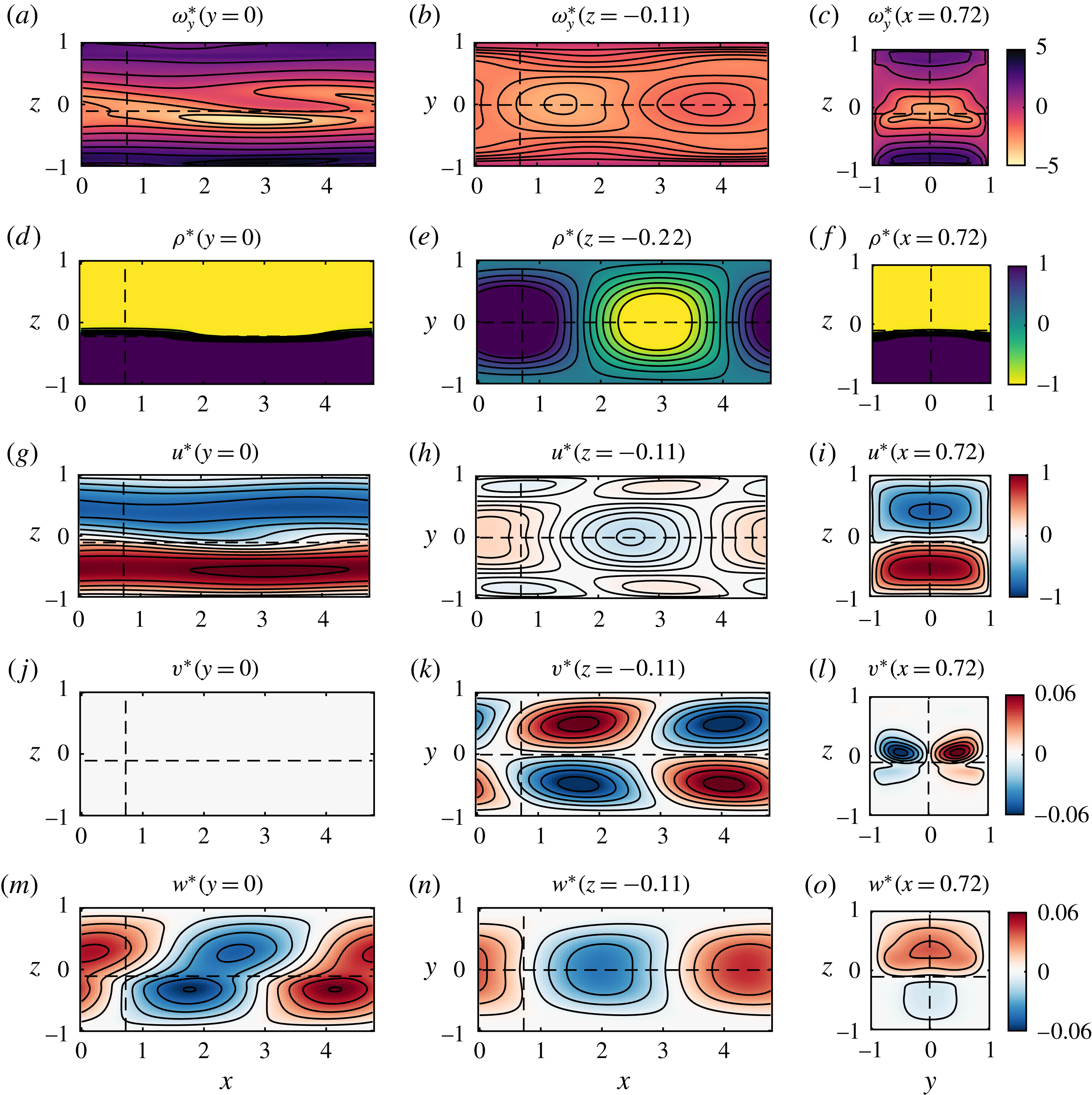
6.2 2P-1B results
6.2.1 Dispersion relation
The dispersion relation of the 2P-1B analysis in shown in figure 6 by the green dotted curve. The fastest-growing ‘traditional’ two-dimensional HI has a growth rate higher than its three-dimensional confined counterpart CHI, at
 $\unicode[STIX]{x1D70E}_{r}=0.173$
, which is achieved at a slightly larger wavenumber
 $k=1.52$
, well within the experimentally range observed.
This mode is almost stationary, with a phase speed of
 $c=0.002$
. This positive value is slightly surprising, as we are dealing with an originally leftward-propagating Holmboe mode. Further inspection reveals that this is an effect of the positive tilt angle
 $\unicode[STIX]{x1D703}=5^{\circ }$
of the duct. Solving with
 $\unicode[STIX]{x1D703}=0^{\circ }$
gives
 $\unicode[STIX]{x1D70E}_{r}=0.215,c=-0.045$
, and we found that a small positive angle decreases the growth rate and increases the phase speed to positive values. These effects are not thoroughly understood, but the behaviour of these linear, inherently two-dimensional modes is not of central interest to our study. In contrast, the wavenumber and phase speed of the CHI predicted by the inherently three-dimensional 3P-2B analysis are not sensitive to the angle. For example, setting
 $\unicode[STIX]{x1D703}=0^{\circ }$
increases the growth rate slightly to
 $\unicode[STIX]{x1D70E}=0.10>0.0824$
but similar
 $k$
and
 $c$
are predicted.
6.2.2 Eigenfunctions
By analogy with the approach followed in § 6.1.2, the one-dimensional vorticity eigenfunction of the fastest-growing mode was added to the one-dimensional base flow such that
 $$\begin{eqnarray}\displaystyle \unicode[STIX]{x1D714}_{y\dagger }^{\ast }\equiv \unicode[STIX]{x2202}_{z}U+\unicode[STIX]{x1D6FC}_{\dagger }\,\text{Re}\{\hat{\unicode[STIX]{x1D714}}_{y\dagger }(z)\exp (\text{i}kx+\unicode[STIX]{x1D719}_{\dagger })\}, & & \displaystyle\end{eqnarray}$$
where the amplitude
 $\unicode[STIX]{x1D6FC}_{\dagger }$
was determined in the same fashion as for the 3P-2B analysis, i.e. by matching the r.m.s. of the vorticity eigenfunction to the experimental perturbation in the mid-plane
 $y=0$
:
 $$\begin{eqnarray}\displaystyle \langle (\unicode[STIX]{x1D714}_{y\dagger }^{\ast }-\unicode[STIX]{x2202}_{z}U)^{rms}\rangle _{x,z}=\langle (\langle \unicode[STIX]{x1D714}_{y}\rangle -\unicode[STIX]{x2202}_{z}U)^{rms}(y=0)\rangle _{x,z}=0.58. & & \displaystyle\end{eqnarray}$$
The other flow variables
 $\unicode[STIX]{x1D70C}_{\dagger }^{\ast },u_{\dagger }^{\ast },w_{\dagger }^{\ast }$
were then obtained using
 $\unicode[STIX]{x1D6FC}_{\dagger }$
similarly to (6.3a
), (6.3b
), (6.3d
) and are shown with
 $\unicode[STIX]{x1D714}_{y\dagger }^{\ast }$
in figure 10.
From figure 10(a), it appears that the ‘head’ of the distinctive vorticity structure observed in the experimental CHW (figure 8
a) and predicted by the CHI (figure 9
a) is lacking. The vertical velocity pattern in figure 10(d) has a similar appearance to figures 8(m) and 9(m) but has a larger amplitude (approximately 60 % larger, requiring different colour bar limits of
 $\pm 0.1$
instead of the previously used
 $\pm 0.06$
). The relative magnitude of the vertical velocity
 $w$
versus the spanwise vorticity
 $\unicode[STIX]{x1D714}_{y}$
(and hence the streamwise velocity
 $u$
) in the 2P-1B analysis is therefore different from the equivalent relative magnitude in the 3P-2B analysis and compares poorly with the experimental observations. Moreover, this analysis is, by construction, incapable of reproducing the three-dimensional structure of the CHW discussed in § 6.1.2, which we have shown depends on the spanwise coordinate
 $y$
and spanwise velocity
 $v$
.

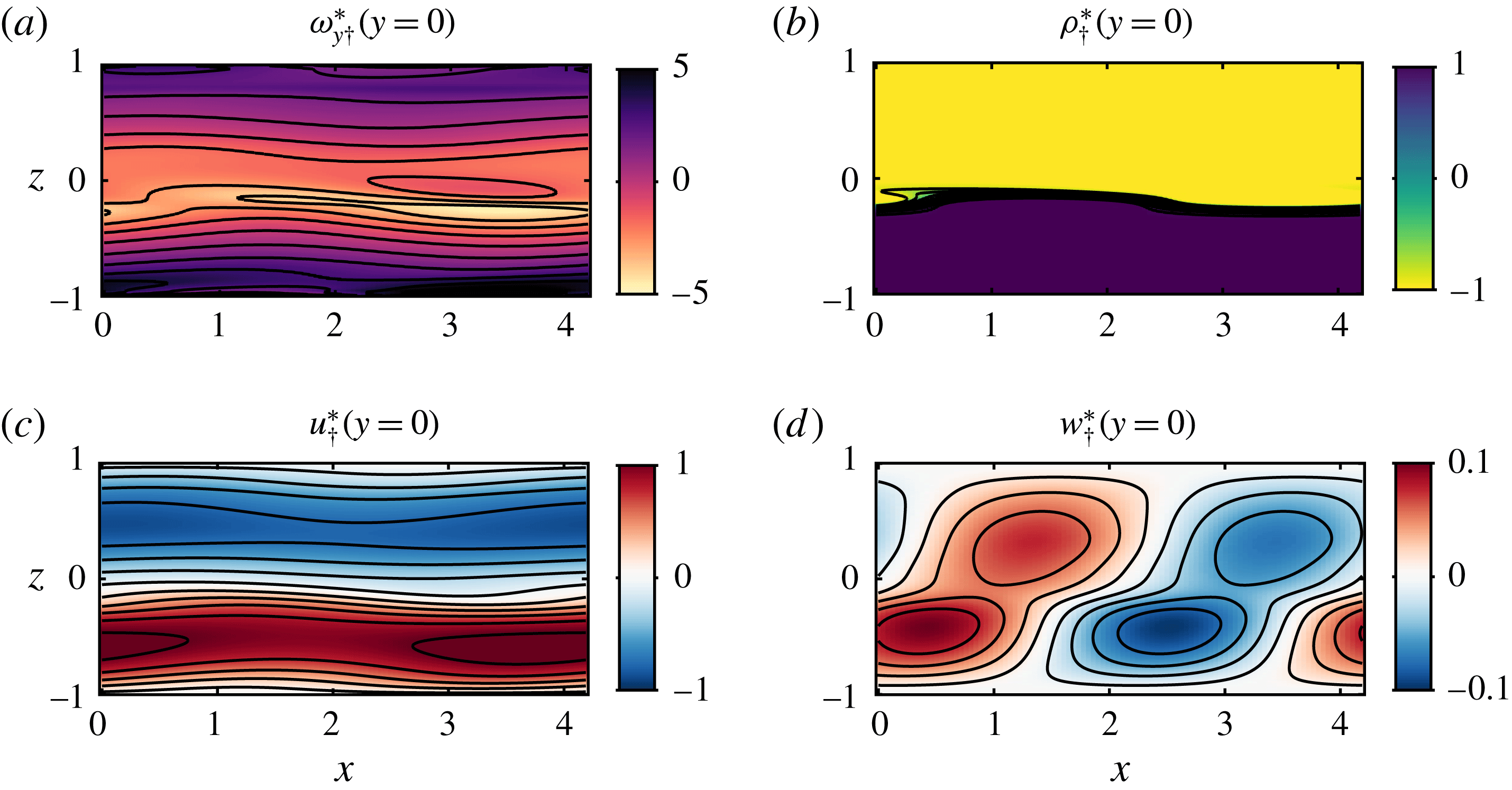
6.3 Possible relevance to geophysical field observations
The distinctive tilde shape of the CHW and CHI is reminiscent of the field observations of Geyer et al. (Reference Geyer, Lavery, Scully and Trowbridge2010) in the continuously forced stratified shear flow of the Connecticut River estuary. Through the combined use of acoustic backscattering and high frequency conductivity sensors around the sharp density interface (pycnocline), they observed a near-periodic signal of large sheared tilde-shaped regions of high density gradients with average wavelength around 10 m and height around 1 m (see their figures 2b and 3b, where the
 $z$
axis has been stretched by factors of 12 and 6, respectively). Those structures are oriented in the same direction as our vorticity structures (the mean shear has the same direction in both our work and their work) and we estimate their maximum angle at the inflection point around
 $5^{\circ }{-}6^{\circ }$
, somewhat smaller than that of the CHW (
 $10^{\circ }$
) and CHI (
 $8^{\circ }$
). They identified these regions as the braids connecting Kelvin–Helmholtz billows, and argued convincingly, in particular from the conductivity measurements, that these inclined ‘braids’ were the locations of the most vigorous turbulent motions, and that the large density gradients resulted from turbulent mixing within the braids, an inherently high-
 $Re$
phenomenon which was unlikely to be observed experimentally or numerically. Mashayek & Peltier (Reference Mashayek and Peltier2012a
,Reference Mashayek and Peltier
b
) identified secondary instabilities localised in the braid regions connecting Kelvin–Helmholtz billows as a possible explanation for the observations of Geyer et al. (Reference Geyer, Lavery, Scully and Trowbridge2010). Here we have identified a primary instability, the CHI, whose finite-amplitude manifestation is also consistent with these observations. Since the background profiles of the estuary flow are not known with sufficient accuracy to distinguish between flows susceptible to the Holmboe instability or flows susceptible to the Rayleigh instability, we cannot eliminate either of these explanations at this stage. However, unlike the simulated secondary braid instabilities of Mashayek & Peltier (Reference Mashayek and Peltier2012a
,Reference Mashayek and Peltier
b
), which occur as a transient event in an initial value problem, the observed CHWs occur in a flow in which the forcing is maintained in time as is the case in the estuary flow.
Preliminary experimental observations of flows in the stratified inclined duct in the intermittently turbulent and fully turbulent regimes revealed a variety of smaller-scale, shorter-lived vorticity structures whose appearance resembles that of the CHW. In particular, two-dimensional (
 $y=0$
) particle image velocimetry measurements at high temporal resolution in the intermittent regime (
 $\unicode[STIX]{x1D703}=4^{\circ },Re=940$
– not reported here) strongly suggest that those small-scale structures appear to come from the cascade break-down of larger-scale structures akin to the CHW through successive stretching and splitting.
We, therefore, argue that it is at least possible that the angled structures we observed experimentally (CHW) and predicted theoretically (CHI), through their local coherent intensification of spanwise vorticity due to the spanwise confinement, also have the potential to leave a ‘signature’ at higher
 $Re$
, even when incoherent, turbulent small-scale motions have been triggered. In particular, in the spirit of the dynamical systems approach discussed in the introduction, we conjecture that the CHW might be sufficiently robust, even at substantially higher
 $Re$
, to constitute an alternative nucleation site for secondary instabilities and hence turbulent break-down, distinct from the strained braid-like region that occurs between finite-amplitude Kelvin–Helmholtz billows proposed by Corcos & Sherman (Reference Corcos and Sherman1976) and invoked by Geyer et al. (Reference Geyer, Lavery, Scully and Trowbridge2010).
7 Conclusions
7.1 Summary
We have investigated the structure and origin of a ‘confined Holmboe wave’ (CHW), a finite-amplitude, nonlinear wave at the sharp density interface of a sustained stratified shear flow.
The stratified inclined duct experiment (figure 1) sets up an exchange flow in an inclined square duct connecting two reservoirs containing fluids of different densities. The flow is steadily forced by gravity for hundreds of advective time units, and can maintain relatively high levels of dissipation, as measured by the buoyancy Reynolds number
 $Re_{b}$
(see (2.1)). By setting the duct tilt angle
 $\unicode[STIX]{x1D703}$
and the density difference
 $\unicode[STIX]{x0394}\unicode[STIX]{x1D70C}$
between the two reservoirs connected by the duct (and hence the Reynolds number
 $Re$
, see (3.4)), different flow states are observed. For
 $20\lesssim Re\sin \unicode[STIX]{x1D703}\lesssim 50$
, a coherent wave state features robust, propagating symmetric or asymmetric Holmboe waves (HWs), confined within the square cross-section of the duct. In order to characterise the structure of CHWs, we focused on the simpler case of upward-pointing, asymmetric HWs found in a flow in which
 $\unicode[STIX]{x1D703}=5^{\circ }$
and
 $Re=440$
.
We employed a novel time-resolved, near-instantaneous measurement technique of the three-component velocity field
 $(u,v,w)$
(stereo particle image velocimetry) and density field
 $\unicode[STIX]{x1D70C}$
(planar laser induced fluorescence) simultaneously over a three-dimensional volume (see figures 2, 3 and supplementary movies 1, 2). This allowed us to reveal the spatio-temporal behaviour of this CHW (figure 4
a,b) by quantifying its range of wavelengths
 $\unicode[STIX]{x1D706}\in [3.5,6.0]$
, or wavenumbers
 $k\in [1.05,1.80]$
(non-dimensionalised by half the duct height) and phase speeds
 $c\in [-0,18,0.05]$
(non-dimensionalised by the layer peak velocity). We first focused on the three-dimensional structure of its spanwise vorticity, where the wave field periodically reinforces and weakens the mean shear to form a pattern of inclined, distorted, prolate spheroids with a wide ‘body’ and a narrower ‘head’ (figure 3). Using phase-averaging we extracted a typical, robust representation of the CHW and characterised its salient features (figure 4
c,d).
To understand the origin (i.e. the underlying physical mechanisms that lead to the observed behaviour) of this apparently previously unreported structure, we undertook a linear stability analysis. We studied three-dimensional velocity
 $(u^{\prime },v^{\prime },w^{\prime })$
and density
 $\unicode[STIX]{x1D70C}^{\prime }$
perturbations having two-dimensional, cross-sectional eigenfunctions of
 $y,z$
and a normal streamwise mode in
 $x$
:
 $\unicode[STIX]{x1D713}^{\prime }\equiv \hat{\unicode[STIX]{x1D713}}(y,z)\exp (\text{i}kx+\unicode[STIX]{x1D70E}t)$
. Those perturbations were analysed on the two-dimensional (
 $y,z$
, i.e.
 $x$
and
 $t$
-averaged) experimental mean flow (figure 5) and were confined with the appropriate boundary conditions in the square duct. This computation revealed the existence of a ‘confined Holmboe instability’ (CHI) with wavenumber band
 $k\in [0.8,2.2]$
, phase speed band
 $c\in [-0.35,-0.08]$
and fastest-growing mode
 $k=1.32$
,
 $c=-0.21$
, consistent with the properties of the CHW (figure 6). By matching the volume-averaged root-mean-square (r.m.s.) of the spanwise vorticity eigenfunction to the experimentally observed value, we reconstructed the three-dimensional structure of the CHI to compare it with the CHW. The side-by-side comparisons of the vorticity isosurfaces (figures 4
c,d and 7
a,b as well as supplementary movie 3) and slices of flow variables
 $\unicode[STIX]{x1D714}_{y},\unicode[STIX]{x1D70C},u,v,w$
(figures 8 and 9) show excellent agreement between the finite-amplitude wave and the predicted instability. These views revealed further details including the spanwise mid-duct localisation, the convexity of the density crests and troughs, the resulting localisation of the baroclinic production of vorticity, as well as the divergence/convergence of the flow around density crests, causing vortex stretching. Such localisation and stretching are inherent to the spanwise confinement and are believed to play a critical role in the dynamics of the CHI/CHW.
We also compared these results with those of the more commonly used stability analysis of two-dimensional perturbations
 $(u^{\prime },w^{\prime },\unicode[STIX]{x1D70C}^{\prime })$
with an associated one-dimensional eigenfunction in
 $z$
and a streamwise normal mode in
 $x$
of the form
 $\unicode[STIX]{x1D713}_{\dagger }^{\prime }\equiv \hat{\unicode[STIX]{x1D713}}_{\dagger }(z)\exp (\text{i}kx+\unicode[STIX]{x1D70E}t)$
on the one-dimensional, mid-duct base flow. Despite the dispersion relation showing some agreement (figure 6), the two-dimensional predicted structure (figure 10) compares less favourably with the experimental results and fails, by construction, to capture any spanwise confinement and behaviour. Crucially, the spanwise velocity perturbation
 $v^{\prime }$
of the CHI is an odd function of the spanwise
 $y$
coordinate, possessing a different spanwise periodicity from the other perturbation variables. This key property cannot be captured by such purely one-dimensional eigenfunctions, or even by normal modes ‘propagating at an angle’ to the base flow.
Finally, the coherent structure associated with the CHW bears a passing resemblance to the distinctive angled structures observed in the Connecticut River Estuary by Geyer et al. (Reference Geyer, Lavery, Scully and Trowbridge2010). While perhaps fortuitous, this resemblance, as well as preliminary experimental results in more turbulent flows not reported here, lead us to conjecture that the angled coherent structures of the CHW may retain at least a partial signature in higher-
 $Re$
flows with lateral confinement and sharp density gradients.
7.2 Future directions
Our results raise a number of questions that may stimulate future research.
(i) How generic is the effect of confinement on shear flow instabilities? This paper focused on an asymmetric Holmboe wave found in a particular laboratory flow, and four additional experiments with similar parameters confirmed that the qualitative results outlined in this paper are robust. Asymmetric HWs might be more generic than symmetric HWs due to some inevitable degree of asymmetry present in environmental flows; however, they introduce another non-dimensional parameter (the degree of asymmetry) to the problem. More work is needed to investigate the effect of confinement in the parameter space spanned by HWs. Varying the level of confinement by considering rectangular ducts or other geometries would add further complexity but may be worth pursuing. Moreover, little work has been done to study the effect of confinement on other instabilities, such as the so-called Kelvin–Helmholtz instability. As outlined in our review in § 2, laboratory observations in confined geometries are often compared to stability analyses that ignore confinement, and numerical simulations usually impose periodic boundary conditions in the spanwise direction. The results presented here, as well as other preliminary results, suggest that the properties of three-dimensional confined waves may differ significantly from those predicted by such analyses.
(ii) How is the amplitude of the CHW determined and sustained in time? The quasi-steady forcing provided by the stratified inclined duct experiment sustains the observed CHW at an approximately constant amplitude for hundreds of advective time units. We determined this amplitude by computing the volume-averaged r.m.s. of the phase-averaged vorticity perturbation, and used it to compare with the most unstable linear eigenfunction. We did not address the value of this amplitude, which is selected through inherently nonlinear processes. By examining the structure of the CHW, we suggested possible nonlinear vorticity dynamics mechanisms (which rely on confinement) to sustain this wave (i.e. baroclinicity and vortex stretching) but their details and quantitative impact fall outside the scope of this paper. The relatively well-defined parameter range for which the CHW is observed is also particularly interesting. The wave studied here at
$\unicode[STIX]{x1D703}=5^{\circ }$
,
$Re=440$
would be replaced by intermittent turbulence at slightly higher angles
$\unicode[STIX]{x1D703}\gtrsim 6^{\circ }$
and/or values of
$Re\gtrsim 600$
. This suggests that the amplitude of this wave results from a fine-tuning of energy input (through
$\unicode[STIX]{x1D703}$
) and dissipation (through
$Re$
), and that the dissipation that the CHW structure can generate through higher amplitudes is no longer enough beyond a certain threshold in the
$\unicode[STIX]{x1D703}{-}Re$
plane, at which it must bifurcate to more dissipative, intermittently turbulent, structures (Meyer & Linden Reference Meyer and Linden2014; Lefauve Reference Lefauve2018).(iii) Is the coherent structure of the CHW dynamically relevant to more turbulent flows? Does this structure generically emerge in miniature around the fine-scale density gradients of high Reynolds number and high Schmidt number confined flows such as estuarine flows discussed above? Can the large-scale coherent intensification of vorticity catalyse the formation of nucleation sites for secondary instabilities and turbulent break-down? These considerations are central to the dynamical systems modelling mentioned in § 1, using a reduced set of exact coherent states (ECSs), i.e. exact (yet unstable) nonlinear solutions of the Navier–Stokes equations. Recently, Lucas et al. (Reference Lucas, Caulfield and Kerswell2017) successfully converged two ECSs from direct numerical simulations of body-forced, horizontally sheared stratified turbulence in a triply periodic domain. These ECSs were found to be striking representations of the mean flow and could account for the organisation of the stratified turbulence into inclined shear layers. By constructing a bifurcation diagram, they demonstrated that the ECSs originate from a sequence of instabilities, including the stratified linear instability of the base flow. Our results suggest that the experimental long-lived coherent structure of the CHW originates from the linear CHI, but it is still unknown whether it is the signature of a relatively robust ECS that would carry its dynamical significance into confined stratified turbulent flows at geophysically relevant scales. We believe that this question warrants further investigation.


Acknowledgements
We acknowledge the support of EPSRC under the Programme Grant EP/K034529/1 ‘Mathematical Underpinnings of Stratified Turbulence’ (MUST). We thank J. Taylor, R. Kerswell and the rest of the ‘MUST team’ for valuable discussions, as well as L. Lesshafft for suggesting the 3P-2B stability analysis. We are deeply indebted to the technicians of the G. K. Batchelor laboratory, D. Page-Croft, P. Mitton, C. Hitch, J. Milton and A. Denson for their craftsmanship. The data associated with this paper can be found in the repository https://doi.org/10.17863/CAM.21932.
Supplementary movies
Supplementary movies are available at https://doi.org/10.1017/jfm.2018.324.
Appendix A. Derivation of the 3P-2B eigenvalue problem
We start by combining the divergence of the linearised momentum equation (5.1b ) and the linearised continuity equation (5.1a ) to obtain a diagnostic equation for the pressure perturbation:
 $$\begin{eqnarray}\displaystyle -\unicode[STIX]{x1D6FB}^{2}p^{\prime }=2(\unicode[STIX]{x2202}_{y}U\unicode[STIX]{x2202}_{x}v^{\prime }+\unicode[STIX]{x2202}_{z}U\unicode[STIX]{x2202}_{x}w^{\prime })+Ri(\cos \unicode[STIX]{x1D703}\,\unicode[STIX]{x2202}_{z}\unicode[STIX]{x1D70C}^{\prime }-\sin \unicode[STIX]{x1D703}\,\unicode[STIX]{x2202}_{x}\unicode[STIX]{x1D70C}^{\prime }). & & \displaystyle\end{eqnarray}$$
We proceed to use (A 1) in combination with the Laplacian of the linearised momentum equation, in order to eliminate
 $p^{\prime }$
. This reduces the dimensionality of our system by increasing its order. The resulting linear system (A 2) fully describes the time evolution of the perturbations using prognostic equations (A 2b
)–(A 2d
) for two velocity variables
 $v^{\prime }$
and
 $w^{\prime }$
and density
 $\unicode[STIX]{x1D70C}^{\prime }$
. The streamwise velocity perturbation
 $u^{\prime }$
is recovered independently by continuity (A 2a
):
 $$\begin{eqnarray}\displaystyle \unicode[STIX]{x2202}_{x}u^{\prime } & = & \displaystyle -\unicode[STIX]{x2202}_{y}v^{\prime }-\unicode[STIX]{x2202}_{z}w^{\prime },\end{eqnarray}$$
 $$\begin{eqnarray}\displaystyle & & \displaystyle \{(\unicode[STIX]{x2202}_{t}+U\unicode[STIX]{x2202}_{x})\unicode[STIX]{x1D6FB}^{2}+(\unicode[STIX]{x2202}_{zz}U-\unicode[STIX]{x2202}_{yy}U)\unicode[STIX]{x2202}_{x}+2\unicode[STIX]{x2202}_{z}U\unicode[STIX]{x2202}_{xz}-Re^{-1}\unicode[STIX]{x1D6FB}^{4}\}v^{\prime }\nonumber\\ \displaystyle & & \displaystyle \quad =2(\unicode[STIX]{x2202}_{yz}U\unicode[STIX]{x2202}_{x}+\unicode[STIX]{x2202}_{z}U\unicode[STIX]{x2202}_{xy})w^{\prime }\nonumber\\ \displaystyle & & \displaystyle \qquad +\,Ri(\cos \unicode[STIX]{x1D703}\,\unicode[STIX]{x2202}_{yz}-\sin \unicode[STIX]{x1D703}\,\unicode[STIX]{x2202}_{xy})\unicode[STIX]{x1D70C}^{\prime },\end{eqnarray}$$
 $$\begin{eqnarray}\displaystyle & & \displaystyle \{(\unicode[STIX]{x2202}_{t}+U\unicode[STIX]{x2202}_{x})\unicode[STIX]{x1D6FB}^{2}+(\unicode[STIX]{x2202}_{yy}U-\unicode[STIX]{x2202}_{zz}U)\unicode[STIX]{x2202}_{x}+2\unicode[STIX]{x2202}_{y}U\unicode[STIX]{x2202}_{xy}-Re^{-1}\unicode[STIX]{x1D6FB}^{4}\}w^{\prime }\nonumber\\ \displaystyle & & \displaystyle \quad =2(\unicode[STIX]{x2202}_{yz}U\unicode[STIX]{x2202}_{x}+\unicode[STIX]{x2202}_{y}U\unicode[STIX]{x2202}_{xz})v^{\prime }\nonumber\\ \displaystyle & & \displaystyle \qquad +\,Ri\{-\cos \unicode[STIX]{x1D703}\,(\unicode[STIX]{x2202}_{xx}+\unicode[STIX]{x2202}_{yy})-\sin \unicode[STIX]{x1D703}\,\unicode[STIX]{x2202}_{xz}\}\unicode[STIX]{x1D70C}^{\prime },\end{eqnarray}$$
 $$\begin{eqnarray}\displaystyle \{\unicode[STIX]{x2202}_{t}+U\unicode[STIX]{x2202}_{x}-(Re\,Sc)^{-1}\unicode[STIX]{x1D6FB}^{2}\}\unicode[STIX]{x1D70C}^{\prime }=-\unicode[STIX]{x2202}_{z}R\,w^{\prime }. & & \displaystyle\end{eqnarray}$$
We now transform the differential operators in
 $x$
and
 $t$
using our ansatz (5.3) (
 $\unicode[STIX]{x2202}_{x^{n}}=(\text{i}k)^{n}$
,
 $\unicode[STIX]{x2202}_{t}=\unicode[STIX]{x1D70E}$
), reducing (A 2b
)–(A 2d
) to the eigenvalue problem (5.4) and (A 2a
) to (5.6).