

Introduction
The regular collection of household survey income data and cross-national harmonisation of income variables has maintained the reliance on disposable income as a defining indicator for economic living standard assessments (Atkinson and Marlier, Reference Atkinson and Marlier2010; Hedström and Ringen, Reference Hedström and Ringen1988; Rigg and Sefton, Reference Rigg and Sefton2006; Wilkins, Reference Wilkins2013). Nevertheless, while disposable income is undisputed as the primary source of current individual purchasing power, it remains an insufficient indicator because it fails to provide a ‘full command over resources’ (Boarini and d'Ercole, Reference Boarini and d'Ercole2006: 10). In seeking to overcome the narrowness of the income metric, scholars have expanded the disposable income measure by imputing an owner-occupier rent (Saunders and Siminski, Reference Saunders and Siminski2005; Smeeding and Weinberg, Reference Smeeding and Weinberg2001; Wolff and Zacharias, Reference Wolff and Zacharias2009); and imputing the value of in-kind public benefits and services (Callan and Keane, Reference Callan and Keane2009; Smeeding et al., Reference Smeeding, Saunders, Coder, Jenkins, Fritzell, Hagenaars, Hauser and Wolfson1993).
These income adjustments are still incomplete because they fail to account for wealth; an economic resource that confers economic security and is a potential source of current and future consumption (Stiglitz et al., Reference Stiglitz, Sen and Fitoussi2009). While some income generated from wealth is picked up in measured disposable income (for instance, through property income in the form of dividends, investment rental flows and royalties), and income metrics can include imputed rent estimates from home ownership, other capital income, such as realised capital gains, are generally not recorded as income but affect consumption possibilities (Stiglitz et al., Reference Stiglitz, Sen and Fitoussi2009). Individuals can increase consumption through dis-savings (reducing wealth) or borrowing irrespective of current income levels (ibid).Footnote 1
Most studies investigate the relationship between income and wealth whilst maintaining the respective income (flow) and wealth (stock) unit status (Bradbury, Reference Bradbury, Gornick and Jäntti2013; Creedy and Tan, Reference Creedy and Tan2007; Radner, Reference Radner1990). Less prevalent are studies that convert income and wealth into the same flow/stock unit to allow aggregation; mostly by supplementing income with a wealth annuity (Brandolini et al., Reference Brandolini, Magri and Smeeding2009; Frick and Headey, Reference Frick and Headey2009; Wolff and Zacharias, Reference Wolff and Zacharias2009). Aggregation of income and wealth into a single metric is advantageous because it enables analysis of the joint distribution of economic resources at the household and (through equivalisation, which assumes intra-household resource-sharing arrangements) at the individual level. A single metric encapsulates the fuller range of economic resources individuals have at their disposal, while retaining the general benefit of a universal numerical money-based metric comparable over time, across groups and against policy targets.
An expanded economic resource approach has international (Stiglitz et al., Reference Stiglitz, Sen and Fitoussi2009) and national endorsement (ABS, 1995). The Australian Bureau of Statistics (ABS) has canvassed the idea of creating a single index, called ‘equivalised wealth-adjusted income’ to identify Australians at risk of economic hardship (Billing et al., Reference Billing, Kindermann, McColl and Rolfe2010). Apart from the initial pioneering work conducted by Travers and Richardson (Reference Travers and Richardson1993), there is no current Australian evidence of empirical attempts to combine an expanded measure of income with wealth into a single metric. This article addresses this concern, by adapting current best practice models (Smeeding and Weinberg, Reference Smeeding and Weinberg2001; Wolff and Zacharias, Reference Wolff and Zacharias2009) to an Australian context and applying the analytic lens to that of older Australians aged 65 years and over.
Older people are a focus because population ageing is postulated as having a profound economic and social effect (Australian Government, 2015). Official reports predict that by 2055, over 22 per cent of the Australian population will be aged 65 years and over. At a macro-level, consideration is given to the challenge for government to mitigate the decreased economic productivity from declining labour force participation rates with the increasing fiscal pressures on publicly funded retirement income, health and aged-care systems (Australian Government, 2015; Australian Treasury, 2009; Productivity Commission, 2011). At a micro-level, consideration is given to maintaining social cohesion across and within generations, with governments playing a critical role in the design and implementation of policies to ensure equity and prosperity to both older and younger Australians. For older people, a key consideration is maintaining the quality of an individual's standard of living over the duration of his or her remaining life span; this, for many, will see them live for decades beyond retirement (ibid).
How we measure the economic standard of living plays a pivotal role in framing public discourse, guiding action around policy responses and, in an era of accountability, is used to assess policy decisions. This article argues that understanding how the full range of economic resources can potentially affect an individual's economic living standards is particularly important in an Australian context, given the high rates of home ownership, the superannuation system and the provision of public in-kind benefits and services.
The next two sections introduce the economic resource metrics and describe the main data sources. The remaining article outlines the methodology to impute the economic resource components and examines the consequences of the newly constructed metrics on the economic living standards of older Australians.
Income concepts
This work combines notions of income and wealth as providing the full array of potential consumption possibilities that determine economic living standards. The term ‘possibilities’ is borrowed from the ABS (Billing et al., Reference Billing, Kindermann, McColl and Rolfe2010: 2), who write that it reflects the capacity to consume rather than a focus on actual or current consumption. The treatment of economic living standards as a function of consumption levels, follows the economic theory that individuals, as rational agents, will consume goods or undertake activities, subject to financial limitation, to maximise their utility/welfare (Atkinson and Marlier, Reference Atkinson and Marlier2010). Referred to as the ‘means of living’ (ABS, 2001: 184), the income-wealth-consumption relationship resonates with the Haig-Simons’ (Haig, Reference Haig and Haig1921; Simons, Reference Simons1938) definition of income as the sum of consumption and the change in net worth over a period. However, unlike Haig-Simons, consumption is not restricted to actual expenditure on goods and services, and income is not inclusive of current and capital receipts of an irregular or non-recurring nature. Instead, the economic resource metrics proposed follow the recommendations of the ABS (1995) and the Canberra Expert Group on Income Statistics (2001). The recommendations restrict income concepts to the current receipt of cash or in-kind income available for current consumption without any reduction in net worth. These metrics, therefore, adopt a wider perspective by examining potential consumption possibilities brought on through the accumulation of income and wealth.
Four economic resource (er) metrics are examined:
 $$\begin{equation}
{\it Disposable\; income}:\;d{y_j}
\end{equation}$$
 $$\begin{equation}
{\it Full\; income}:\;f{y_j} = d{y_j} + st{i_j} + {\rm{\ }}ni{r_j}
\end{equation}$$
stij refers to the value of social transfers in-kind; nirj the net imputed rent from owner-occupied dwellings for household j.
 $$\begin{eqnarray}
{\it Potential\; consumption}:\,p{c_j} & = & (d{y_j} - p{i_j}) + {\rm{\ }}s{i_j} \nonumber\\
&&+\, {\rm{\ }}ni{r_j} + {\rm{\ }}\left( {\mathop \sum \limits_{k = 1}^K nh{w_{jk}}} \right)
\end{eqnarray}$$
pij is property income received from income-generating assets; nhwjk is the constant annuity received from each component of non-housing wealth for all K non-housing wealth components in household j.
 $$\begin{eqnarray}
{\it Adjusted\;potential\;consumption}:\,ap{c_j} & = & (d{y_j} - p{i_j}) + {\rm{\ }}s{i_j} \nonumber\\
&& +\, \ h{w_j} + \left( {\mathop \sum \limits_{k = 1}^K nh{w_{jk}}} \right)
\end{eqnarray}$$
hwj is the constant annuity from owner-occupied housing wealth.
Disposable income (dy), following convention, is confined to cash income items that are regular and recurring (ABS, 2012b). It includes all sources of private income from wages, business, investments, private pensions, private transfers and government cash transfers in the form of pensions and allowances with a deduction for personal income tax. Two income components are added to dy to produce full income (fy): the value of in-kind government social transfers (sti) and the value of net imputed rent (nir) from owner-occupied dwellings. Both are recommended as instrumental components in the income conceptual frameworks set out by the Canberra Group (2001) and by Smeeding and Weinberg (Reference Smeeding and Weinberg2001). Including sti recognises the benefit from the provision of publicly funded health, community, welfare and housing on an individual's living standards (ABS, 2012b; Smeeding et al., Reference Smeeding, Saunders, Coder, Jenkins, Fritzell, Hagenaars, Hauser and Wolfson1993). Including nir recognises that homeowners benefit from having a place to live that allows them to avoid paying the rent incurred by non-home owners (Saunders and Siminski, Reference Saunders and Siminski2005).
Disposable income and full income are measures that affect current consumption. The ‘potential consumption’ metrics acknowledge the role of accumulated assets in providing an income stream that potentially determines the economic living standard achievable (Stiglitz et al., Reference Stiglitz, Sen and Fitoussi2009: 115). Theorised through the Ando-Modigliani life-cycle hypothesis of consumption and saving (Ando and Modigliani, Reference Ando, Modigliani and Franco2005), individuals adjust the pattern of income and wealth accumulation to maintain their marginal utility of consumption over their lifetime (Browning and Crossley, Reference Browning and Crossley2001). Individuals accumulate assets during primary working years when income is higher and run down the stock of assets to finance consumption during retirement when income is lower. It is plausible that people not only consider their current income and savings but their future earnings, borrowing capacity and anticipated wealth creation when they make current consumption decisions (Fisher et al., Reference Fisher, Johnson, Marchand, Smeeding and Torrey2008; Sabelhaus and Schnieder, Reference Sabelhaus and Schnieder1997).
Consequently, the main feature of the third proposed metric (pc) is the addition of annuitised non-housing wealth (nhw) components to the full income metric (fy). Income received from income-generating assets (pi) is deducted from household disposable income to avoid double counting the returns from asset ownership. This is done within the normative income model as an income stream from dividends, rental receipts, interest earned and income generated from private pensions; and within the potential consumption model through the annuitisation of non-housing wealth.
The fourth metric, adjusted potential consumption (apc), replaces the value of nir with a notional annuity from owner-occupied housing wealth (hw). Arguably this is captured (albeit imperfectly) already through nir, and treatment of the house as a liquid asset is problematic (Fisher et al., Reference Fisher, Johnson, Marchand, Smeeding and Torrey2007; Rowlingson, Reference Rowlingson2006). Nevertheless, it remains a useful proposition to consider, given the age-related nature of wealth holdings. For many older Australians, their largest class of asset is the home. Although nir accounts for the services provided by home ownership, it does not include the capital value associated with the home asset. As the ABS (1995: 24) states, ‘the exclusion of non-financial assets and owner-occupied dwellings in particular, would seriously under-estimate the full income potential of the aged’.
Data
To understand the methodological choices, it is necessary to put this article into context. It comprises one part of a broader study that compared economic measures of the standard of living with a multi-dimensional well-being indicator framework at the individual level. In doing so, it examines whether the measured relative position of individuals changes depending on the conceptual approach adopted. The four er metrics, as part of the economic living standards approach, are estimated using the Household Income and Labour Dynamics in Australia (HILDA) Survey. It is currently the only Australian dataset that provides the breadth and depth of economic, social and personal questions at the individual level that are integral to the broader study's scope.
HILDA is a household-based panel study, similar in scope to the British Household Panel Study and the German Socio-Economic Panel. It contains detailed household and person-level data on a range of socio-economic variables including income, wealth, demographics and quality of life indicators, amongst a nationally representative sample of private households. Interviews are conducted with household members aged 15 years and over (known as responding persons). Analysis is restricted to this adult population, with older people defined specifically as respondents aged 65 years and over. To ensure representativeness with Australian population estimates, the sample is weighted using cross-sectional responding person (or, where specified household population) weights.Footnote 2
HILDA is limited, however, with respect to the detailed expenditure and social transfer in-kind data required for the estimation of components of the er metrics. Consequently, where necessary, data is imputed from the 2009–10 ABS Household Income and Expenditure Surveys (HIES) and transposed to HILDA using demographically matched household characteristics (discussion to follow). Analysis is based on wave 10 data as this was the only period for which the HILDA wealth module and the HIES social transfers in-kind were concurrently available at the time analysis commenced.Footnote 3 To provide an estimate of individual economic resources, household data is adjusted to take account of household size and composition using the ‘modified OECD equivalence scale’ (1 to the head of each household, 0.5 to each subsequent adult and 0.3 to each child aged under 15 years).
Imputation of economic resource components
Government social transfers in-kind
HILDA does not contain estimates of sti: hence these values are extrapolated from the 2009–10 ABS Fiscal Incidence Study (FIS) (ABS, 2012a) and transposed at a household level to HILDA. FIS is a formal attempt by the ABS to facilitate household income analysis inclusive of the re-distributive nature of government welfare policies in addition to cash income (ABS, 2012b). ABS FIS allocates public revenue and expenditure from official government national statistics (ABS, 2011c) to individual households within the HIES dataset. It is similar to the conceptual and methodological approach adopted by the UK Office for National Statistics in their Effects of Taxes and Benefits on Household Income publications (ONS, 2016).
Allocation is limited to five functional categories that directly relate to a household's welfare and can be reasonably assigned using household demographic data from HIES: education (pre-school, primary, secondary and tertiary); health (acute care, community health services, pharmaceuticals, private health insurance rebate and other health benefits); social security and welfare (social security and welfare services and child care assistance); public housing (limited to rent subsidies) and a component of fuel and energy (electricity commissions and rebates) (ABS, 2012b: 71). The basic approach is to calculate average benefits based on benchmark estimates for the population group eligible for that specific social transfer in-kind item (ABS, 2012b). For ABS FIS 2009–10, more than 90 per cent of public in-kind expenditures was allocated to individual households in HIES (approximately Aus$157,000 million).
In this article, in-kind items are imputed from HIES to HILDA using ordinary least square regressions that statistically match the demographic characteristics of individuals within each household in both surveys. The dependent variable is the in-kind social transfer item. The independent variables are interaction variables using a combination of age, gender and state categories as specified in HIES and duplicated in HILDA in each household. The coefficients from the HIES-based regression models are then applied to HILDA-based regression models using the same independent variable structure to estimate the imputed sti value for different households in HILDA. This is consistent with the FIS method of allocating expenditure on items according to the utilisation rates of the specific service by a person's age, gender and state of residence multiplied by the average cost for each type of benefit for most items.
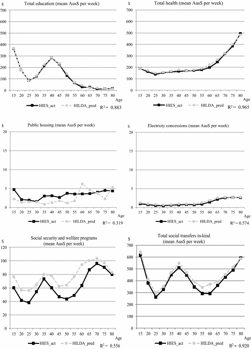
Figure 1 plots the actual weekly mean dollar value of in-kind items in HIES and the corresponding predicted imputed values in HILDA by age for the five functional category totals. The high R2 and the close tracking of the imputed HILDA values to actual HIES expenditures for the majority of sti items reinforce the credibility of the regression-based approach. The exceptions for electricity concessions and social security and welfare services are not unexpected because FIS only allocates expenditure to those identified as recipients of these benefits. These demographic characteristics are not released in the public HIES files or collected in HILDA and hence not included in the regression modelling. Similarly, the income-based eligibility criteria for Australian public housing are not explicitly used as part of the FIS allocation method and therefore not used in this analysis. The imputation of income-based benefit provision within FIS is a concern raised by Harding et al. (Reference Harding, Percival, Schofield and Walker2000) who draw attention to the effect of income levels and socio-economic status and not just age, gender and state on the utilisation of public services. At an aggregate level though, the overall predicative value of the regression is strong with a high R2 of 0.920 and little variation between the recorded total HIES amount and the total imputed sti amount.
Comparison of actual HIES & imputed HILDA social transfer in-kind values by age

Figure 1 also indicates the age-related impact of in-kind benefits. Public education benefits peak for secondary/tertiary students and younger-age people with dependent children, deceasing rapidly thereafter with age. Health benefits increase almost exponentially after 60 years of age. The take-up of benefits received through social security and welfare services shows a series of peaks and troughs with age. A similar pattern is evident for the aggregate across the five categories, as the imputed value for total social transfers in-kind peak for people aged 15–19 years, 35–49 years and 70 years and above.
Net imputed rent for owner-occupied dwellings
Net imputed rent (nir) ‘conceptually treats owner-occupiers as if they were renting their home from themselves, thus simultaneously incurring rental expenditure and earning rental income’ (ABS, 2008: 5). It is conceptually understood as the difference between the notional rent a homeowner would pay to rent his or her home in the private market and the actual costs incurred to maintain and secure ownership of this home. Despite the detailed collection of income and wealth data, nir is not provided as a derived variable within HILDA; with most HILDA-based studies assuming a fixed but arbitrarily chosen percentage of the home value (Rodgers, Reference Rodgers2010; Wilkins, Reference Wilkins2013).
In contrast, in this article, to maintain the integrity of the economic living standard approach, nir is estimated as a two-step process following the ‘market value’ approach (Saunders and Siminski, Reference Saunders and Siminski2005). Gross imputed rent is first estimated by dividing the total amount of gross imputed rent for owner-occupiers listed in National Accounts (ABS, 2011b) by the gross value of owner-occupier homes in HILDA and applying this percentage to the value of each owner-occupier home. The average rate of gross imputed rental return for 2010 is 3.529 per cent of the gross value of the home, based on an estimated Aus$111,742m of gross imputed rent of owner-occupiers (ibid: Table 52) and a HILDA estimate of Aus$3,166b of the gross value of housing stock.Footnote 4
In the second step, nir is estimated as gross imputed rent minus the housing costs associated with maintaining the dwelling. HILDA's housing cost items, however, are limited to one expenditure variable on home repairs, renovations and maintenance. The largest expenditure for owner-purchasers, mortgage interest payments, is excluded. Also excluded are costs associated with building insurance, sewerage and water rates and strata and body corporate fees (referred to as ‘remaining housing costs’). These two housing cost components are calculated as annual rates in ABS HIES 2009–10 and matched to HILDA using the age of the highest income earner in each owner-occupier household as the demographic matching factor between the two datasets.
The ‘mortgage interest payments’ component is calculated as the annual mortgage interest payment as a proportion of the outstanding mortgage debt against the dwelling for each mortgagee household in ABS HIES. The ‘remaining housing costs’ component is calculated as a proportion of the gross current value of the dwelling for each owner-occupier household in ABS HIES. The rates of ‘mortgage interest payments’ (as a proportion of mortgage debt) and the rates of ‘remaining housing costs’ (as a proportion of gross home value) are then applied to each matched owner-occupier household in HILDA to determine nir.
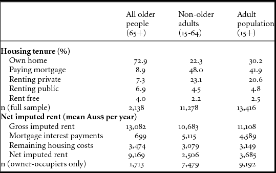
The comparison of tenure patterns and nir by age in Table 1 illustrates the importance of imputing a rent to owner-occupiers and the differential impact of outright ownership on the values of home services received. Net imputed rent is around four times lower for non-older adults driven by an approximately seven-fold increase in ‘mortgage interest payments’ compared to older people but comparable levels of ‘remaining housing costs’. The results corroborate other research by Yates and Bradbury (Reference Yates and Bradbury2010) that older Australians have a large economic resource attached to outright ownership of their home. In keeping with the life-cycle model of wealth accumulation (Browning and Crossley, Reference Browning and Crossley2001), there are three times as many outright owners amongst older people (72.9 per cent) unburdened by mortgage debt compared to non-older adults (22.3 per cent).
Home tenure and net imputed rent comparisons.

Source: Own analysis using HILDA (2010), ABS HIES (2009-10).
Weights: HILDA household and responding person population weights, HIES household population weights.
Annuitising wealth estimates
The potential consumption opportunities afforded through wealth holdings is included in the er metrics in the form of wealth annuities. Wealth is converted into a flow variable using a simple lifetime annuity formula that imputes to the household a fixed annual sum of money for a defined lifetime and reduces wealth to zero at the end of that lifetime (Wolff and Zacharias, Reference Wolff and Zacharias2009). The length of the annuity period is set to the expected remaining life of the household as determined by the age and gender of the youngest adult using ABS life expectancy tables (ABS, 2011a).Footnote 5
The second critical parameter, the real rates of return, is set to reflect the diversity of wealth portfolios by applying Reserve Bank of Australia (RBA) interest rates according to the risk level of each wealth component.Footnote 6 This differs from the conventional use of a single rate of return (such as the standard bond coupon rate) (Brandolini et al., Reference Brandolini, Magri and Smeeding2009; Crystal and Shea, Reference Crystal and Shea1990), which effectively supresses the varying risk levels attached to different wealth components. Financial and superannuation assets have the highest rate of return reflecting the volatility of the share market (3.21 per cent for AA corporate bonds from RBA Table F3). Liquid assets have the lowest rate of return, reflecting the low risk, low return of bank deposits (1.47 per cent from RBA Table F4). The average government bond rate for 2010 (2.69 per cent from RBA Table F2) is applied to home equity as it provides the highest return with the lowest risk. The same rate is applied to the remaining asset and debt classes, which potentially under-estimates their true value in the market but represents a minimum government guaranteed ceiling.
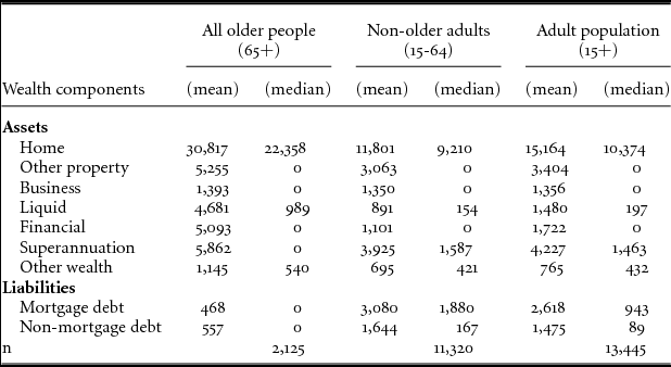
Table 2 shows the age-related impact of including wealth. Mean annuity values are higher across all asset components, except for business assets, for older people when compared with non-older adults, with correspondingly much lower debt annuity values. Apart from the home and liquid asset, the differential age impact is less evident when comparing median values. The disparity between mean and median annuities for older people is evidence of a small group with high levels of non-housing wealth, in addition to home ownership, inflating the mean. Most older people have little or no debt with most wealth held through outright home ownership and, for a few, in liquid form.
Wealth annuities (equivalised mean and median Aus$ per annum).Footnote 7

Source: Own analysis using HILDA.
Notes: Wealth components include: liquid (bank accounts, cash and life insurance); financial (equity investments and trust funds); other wealth (collectives and vehicles); and non-mortgage debt (relating to business, other property, credit cards, personal and overdue household bills).
Main findings
Relationship between the er metrics
In Table 3 the varying range in pair-wise correlation coefficients between the metrics, for both non-older adults and older people, provides empirical evidence supporting the conceptual rationale for an expanded economic resources approach. High correlations between dy and fy is understandable as fy includes dy as its major component (on average for the adult population dy constitutes 76.7 per cent of fy). A similar rationale holds for high correlations between pc and apc. However, correlations between the remaining combination of metrics, (dy and pc/apc; fy and pc/ap), are lower for non-older adults (0.81 to 0.84) and substantially lower for older people (0.49 to 0.69). The range in estimates suggest that the addition of economic resource components, particularly wealth, captures a potential economic resource portfolio not linked to disposable income. Importantly, it is not the same individuals who perform well across the four metrics.
Correlations between economic resource metrics.

Note: Pearson correlation coefficients significant at ρ < 0.05*. Null hypothesis - no linear relationship between each pair of variables.
Median values and relative rates
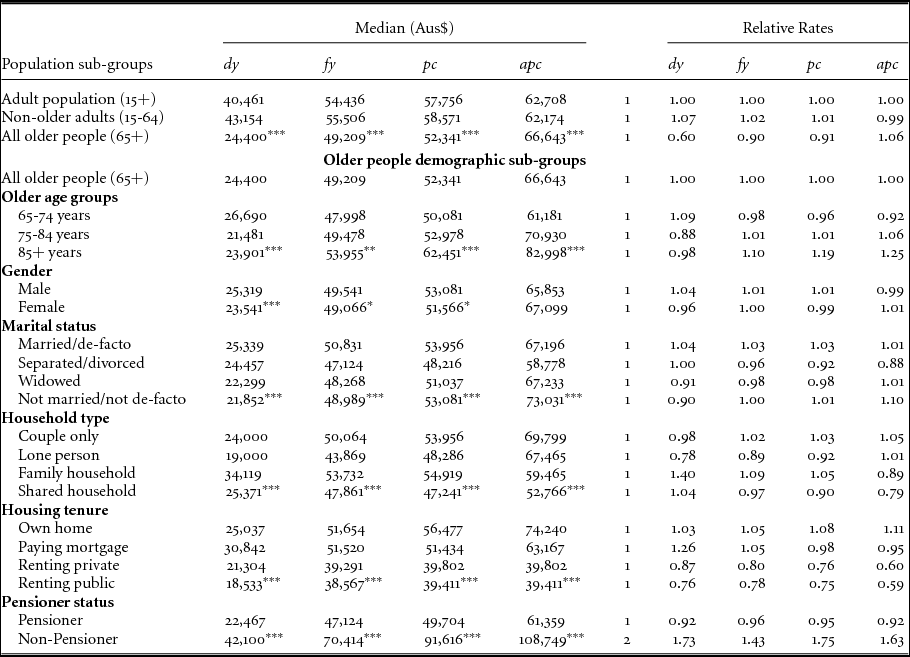
Table 4 presents the median estimates for the er metrics for different population sub-groups. The relative rates in the last four columns compare the median estimates of older people and non-older adults to all adults (shaded top panel) and demographic sub-groups of older people compared to all older people (non-shaded bottom panel).
Economic resource metric estimates and relative rates.

Note: (a) Kruskal Wallis test of significant difference in medians at ρ < 0.05*, 0.01** and 0.001***. (b) Last four columns, lines 3-5 cells indexed to all adults (line 3); all other lines cells indexed to all older people (line 7).
At an aggregate level, the results (shaded top panel) reveal the considerable improvement in the overall economic position of older people with each metric. While comparisons of disposable income support the proposition (evidenced in disposable income-based literature (Harding et al., Reference Harding, King and Kelly2002; OECD, 2009)) that older people are disadvantaged compared to the rest of the population, the argument is weakened as the metrics are expanded to include publicly provided services and wealth. From having a relative dy median ratio of 0.60, this increases to 0.90 (fy) when non-cash benefits and then wealth is included in the form of the pc metric (0.91).
It is the inclusion of the capital value in home wealth, though, that is the catalyst for the step change improvement in the measured relative economic position of older people compared to non-older adults. Without accounting for the capital value of the home, the largest contributors to wealth portfolios across the older age spectrum are superannuation and other property (see Table 2). However, the consequence of high rates of outright home ownership amongst many older Australians means that adding the annuitised value of home wealth increases the relative median rate to above that of non-older adults (apc = 1.06 compared to 0.99).
Based on the dy metric, the pattern of results for sub-groups of older people (non-shaded bottom panel) is consistent with conventional analysis (Harding et al., Reference Harding, King and Kelly2002; OECD, 2009): older old (75+ years) people; females; unmarried or widowed old people; couple only and lone person households; pensioners and renters have lower median dy ratios than the aggregate. There is an obvious correlation in these results related to gender and age; females live longer and consequently are more likely to be widowed, live alone, have retired from (or never been attached to) the workforce and are, therefore, more dependent than males on the Age Pension as their primary income source (OECD, 2009). Conversely, the generalised explanations for younger old people, older males, married and older couple households stem from many interacting factors. Older males, unencumbered by care responsibilities and broken work patterns along the life course, benefit from higher incomes and longer working lives (ibid). Prevalent also are economies of scale as married/couple older people can potentially share resources.
However, different conclusions are reached when analyses are based on fy, pc and apc. Gender differences diminish and are not as significant. The relative disposable income advantage of younger old people (65-74) compared to older old people (75 years and over) is not sustained once the impact of increased age-related health needs and increased pension-related social and welfare services is accounted for through sti. At a household level, there is also the coupling of accumulated wealth over the life course, particularly outright home ownership, with shorter remaining life spans that provide older old people with higher wealth annuities in the pc and apc metrics.
Changes in the relative economic position with each er metric indicates a more entrenched and polarised division between the relative economic advantage of home owners to the relative disadvantage of older renters, and similarly of married older people to divorced/separated older people. Results for widowed older people and those living alone are understandable, as two-thirds of those living alone are widowed.Footnote 8 The relative economic position of widowed older people reflects the relationship consequences of asset ownership/division over the life course. Similarly, the relative economic position of older people in family and shared households reflects the life-cycle accumulation of wealth and income of older individuals themselves and the remaining household members.Footnote 9 The income gains from including the disposable income of working-age members dissipates once the comparative value of their accumulated wealth (or lack of) is considered. Finally, the sustained advantageous position of non-pensioners is not unexpected as further analysis of this sub-group reveals a synergistic relationship between age, income and wealth. Approximately 75 per cent of them are aged between 65–74 years, with around 35 per cent attached to the labour force.Footnote 10 In addition to higher income levels, wealth levels are substantially higher, around 3.5 times that of pensioners, with larger proportions of wealth stemming from investments in non-home property, financial assets and superannuation.
Quintile distributions
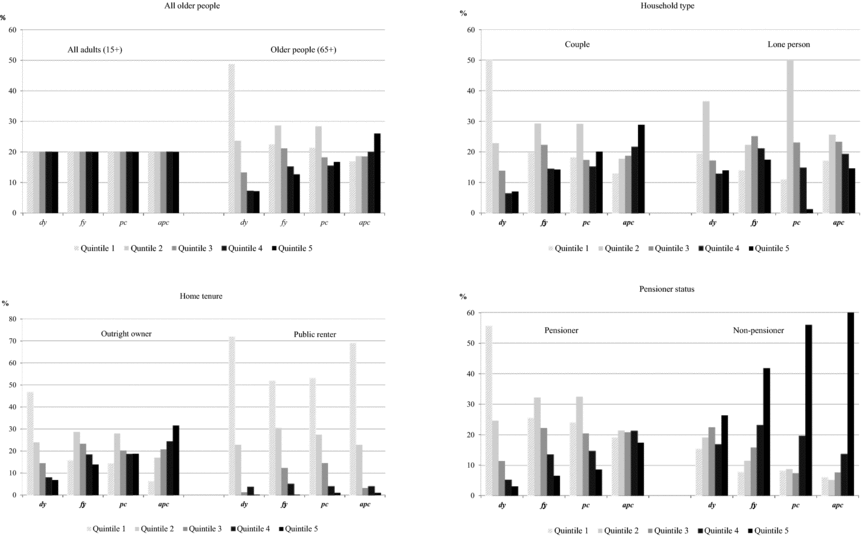
To provide a nuanced understanding of the distributional consequences of the metrics, Figure 2 plots the quintile distribution of all older people and specific sub-groups using the quintile thresholds of the full adult (15+) population for each er metric. The most pronounced finding is the noticeable change in the relative position along the quintile distribution of all older people with each metric. While older people are disproportionately represented in quintiles 1 and 2 (over 70 per cent) through the dy lens, the effect of the economic resource components in the fy metric has an equalising effect on the distribution, supporting findings that non-cash benefits are predominantly ‘pro-poor’ (Callan and Keane, Reference Callan and Keane2009; Verbist and Matsaganis, Reference Verbist, Matsaganis and Vandenbroucke2014). Aligned with the findings based on median relative ratios, the impact of wealth beyond that is to gradually shift the distribution of older people upwards to more closely resemble the quintile distribution of the adult population.
Distribution of older people and sub-groups of older people by adult population er quintile (%)

There are four key findings in relation to demographic sub-groups illustrated below. First, reverses in the bottom and top quintile distributions for lone person households is evidence of a small group (including widowers) with high levels of wealth but low levels of disposable income. Second, quintile distributions reinforce the polarised position of home owners to renters. For public renters, although there are slight reductions in quintiles 1 and 2 with each metric, the combined proportion in quintiles in 4 and 5 never exceeds 6 per cent. Conversely, the changing distributional profile for home owners suggests that it is not just home ownership that drives higher mean wealth levels, but a compounding wealth effect from investments in non-home assets.
Third, the intensified advantageous economic position of non-pensioners with each er metric corroborates Table 3 results. Fourth, the high representation of pensioners amongst the bottom dy quintiles is not unexpected given that the provision of the public pension through the Australian retirement income system is not targeted towards income replacement (social insurance) but a safety net providing minimum income levels (social assistance) (Yates and Bradbury, Reference Yates and Bradbury2010). However, similar proportions across the fy and pc quintiles suggest a small group of pensioners with access to non-home wealth (inflating sub-group mean values) that are either below the pension assets threshold or don't yield high income streams (similar to Creedy and Tan's (Reference Creedy and Tan2007) conclusions).
Reviewing the er metrics
The er metrics illustrate the importance of accounting for the inter-relationship between income, (cash and non-cash forms) and wealth in economic living standard analyses. Nevertheless, inclusion of imputed social transfers in-kind and annuitised home wealth are contentious and require further discussion.
Criticism with sti centres on the implicit assumption that the larger the allocation of benefits to the individual, the better their overall standard of living (Callan and Keane, Reference Callan and Keane2009; Radner, Reference Radner1997). This is problematic in relation to the increased allocation of public health expenditures for older people from the natural onset of increasing health issues, and the increased allocation of public education expenditures to students and families with school-aged children. Despite the inherent characteristic of age-specific provision of public in-kind services, it is possible to mitigate some of the pronounced relationship between those with the greatest need receiving the greatest imputed benefit value.
One approach is to apply equivalence scales that account for differences in need (see Atkinson and Marlier, Reference Atkinson and Marlier2010; Radner, Reference Radner1997; Verbist and Matsaganis, Reference Verbist, Matsaganis and Vandenbroucke2014), although the conceptual and computational complexity in determining how needs vary along the life course has precluded this application within routine economic living standard analyses (ABS, 1995: 26). Another approach, utilised by the ABS FIS, is to not allocate expenditure according to actual usage rates but use average utilisation rates by age, gender and state, following the ‘risk-related insurance approach’ employed by insurance companies (Callan and Keane, Reference Callan and Keane2009: 51). Hence, you can technically be a healthy older person and have the same imputed health benefit as a sicker older person.
From an economics resource perspective there is the consideration, however, that without state provision of welfare benefits and services, these costs would otherwise be borne by individuals with specific needs and paid from their after-tax cash income. The public provision of welfare is, therefore, treated as a notional ‘saving’ to the consumer of the benefit or service. It forms a critical element in the economic decision-making of many individuals and households as the largesse of the welfare state affects their ability to fund discretionary spending. By not accounting for it, a major contribution to maintaining a decent economic living standard for many Australians is ignored.
Criticism against including annuitised home equity rests on the practical plausibility of divesting one's home in later life to fund consumption opportunities. There are financial constraints with asset illiquidity and high purchasing transaction costs (Rowlingson, Reference Rowlingson2006) and barriers to releasing housing equity (Jefferson et al., Reference Jefferson, Austen, Ong, Haffner and Woods2017). There are emotional constraints driven by bequest motives and the psychological attachment to one's home (Colic-Peisker et al., Reference Colic-Peisker, Johnson, Smith, Smith and Searle2010; Fisher et al., Reference Fisher, Johnson, Marchand, Smeeding and Torrey2007; Olsberg and Winters, Reference Olsberg and Winters2005). In Australia, there are major policy features that promote retaining wealth in the home, such as the exemption of owner-occupied housing from capital gains and land tax, and the lack of an inheritance tax (Australian Treasury, 2009). More important is the exclusion of the value of the principal place of residence from the assets tests for receipt of the Age Pension (Productivity Commission, 2011).
Consequently, despite the heterogeneity of housing types and individuals within the population, irrespective of individual disposable income levels, it is the only asset class that most people own and is the main vehicle of their saving. But unlike other assets in a wealth portfolio, the home asset has a unique dual role, functioning simultaneously as a source of realisable wealth and a source of consumption services (Elsinga and Mandič, Reference Elsinga and Mandič2010). It is both an ‘investment good and a consumption good’ (Dietz and Haurin, Reference Dietz and Haurin2003: 411).
Acknowledgment of the potential economic resource held within home equity has led to many policy recommendations about accessing it. Australian policy debates include: abolishing stamp duty; introducing a bequest tax; deeming an income beyond an asset threshold for income benefit eligibility; including the value of the home above a certain threshold in the Age Pension means test; and providing a government guaranteed home-equity release scheme to fund aged-care expenses (Australian Treasury, 2009; National Commission of Audit, 2014; Productivity Commission, 2011), with no consensus on the best outcome for all Australians. Within these policy contexts, including the full value of annuitised home wealth through the apc metric represents an upper bound. It provides a lens to gauge the full impact of home ownership and other forms of asset ownership (‘stocks’) within an income ‘flow’ dimension, on an individual's economic standard of living.
Conclusion
Disposable income, although important, is conceptually limited as a means of assessing economic living standards. This article treats economic living standards as a function of income (cash and non-cash) and wealth as economic resources that determine potential consumption possibilities. Augmenting disposable income with income streams from non-cash services and annuitised wealth substantially improves the measured relative aggregate economic position of older Australians compared to non-older adults.
Moreover, this paper generates different conclusions about the relative economic position of demographic sub-groups of older people that are otherwise drawn using the disposable income metric. With each full income, potential consumption and adjusted potential consumption metric, the relative economic position of younger old to older old people, males to females, couple to lone person households and married to widowed older people are brought closer to parity with each other. Conversely, they indicate a widening gap between the economic advantage of home owners and corresponding disadvantage of older renters, and similarly the polarised position between married and divorced/separated older people. The results suggest that it is the combination of three features unique to the current Australian policy environment that benefits many within this cohort of older Australians: the provision of a minimum income standard through the Age Pension; the financial benefits (and tenure security) from home ownership; and equitable and adequate access to health, aged care and community services.
The fy, pc and apc metrics are proposed as viable analytic alternatives to dy on the basis that it is conceptually desirable, empirically informative and necessary for policy development. They are by no means perfect, excluding important components such as the value of home production, leisure, employee non-cash benefits and a more rigorous asset transaction assessment. However, social scientists have long recognised that the measurement of income and wealth is by nature a ‘rough-and-ready process and always contains errors’ (Travers and Richardson, Reference Travers and Richardson1993: 175). The metrics function as a conceptual ‘thought’ experiment, highlighting the need for integrated policy discussion and debate about the collective role that income, public services and wealth have on maintaining the economic living standard of this generation of older Australians while ensuring the same access to and level of provisions for future generations.