3.1. Sampling phase

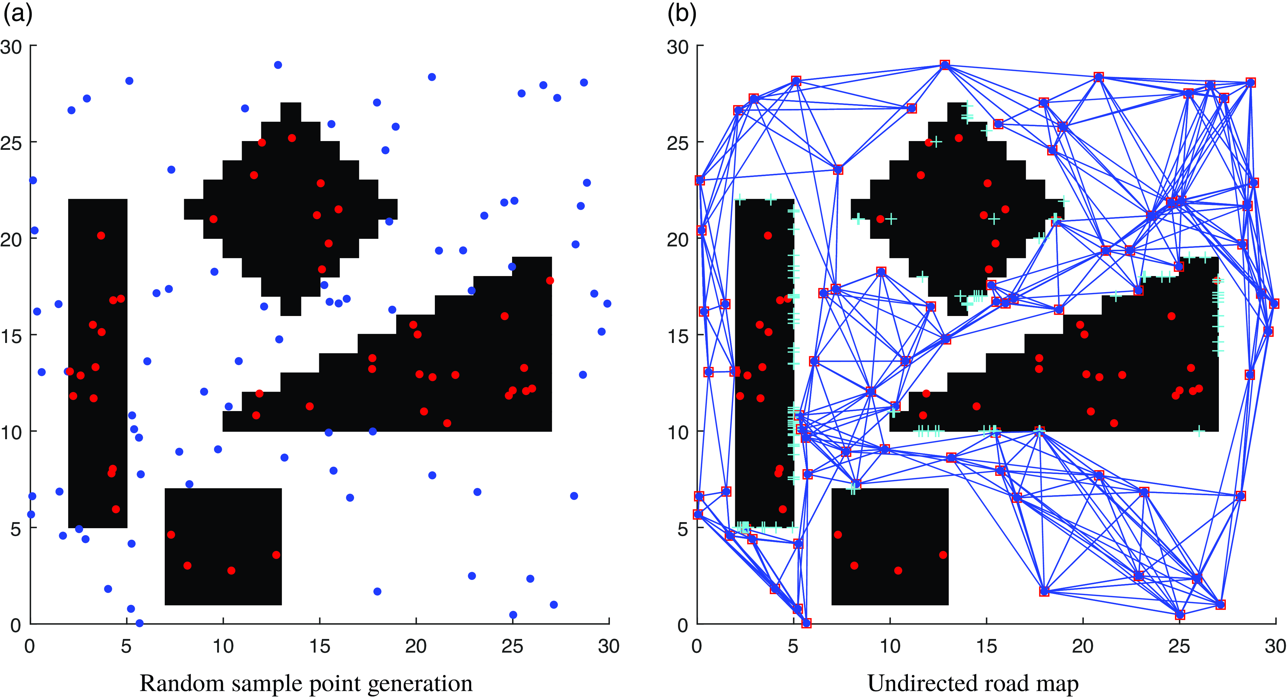
In the sampling stage of PRM algorithm, a certain number of random sampling points are first generated in the map space. Collision detection is performed for each sampling point to exclude points located within obstacles, ensuring that all nodes are in free space (see Figure 1(a)). Next, for each valid sampling point, the algorithm searches for other sampling points within the connection threshold. It determines if these points can be connected by a straight line. The algorithm ensures that this line does not cross any obstacles. These valid connection edges are added to a graph, forming an undirected roadmap (see Figure 1(b)). Here, $V = \left \{ v_1,v_2,\dots,v_n \right \}$ denotes the set of nodes, and $E = \left \{ v_i,v_j|v_i,v_j\in V \right \}$ denotes the set of edges between nodes. The primary goal of the sampling stage is to generate a graphical structure. This structure is based on environment modeling and can effectively represent the valid paths of the robot within the environment. Subsequently, in the path search stage, the roadmap (G (V, E)) can be used. It allows for the quick identification of effective paths. This capability accelerates the path search and planning process.

Figure 1.

Sampling stage.

3.2. Query phase

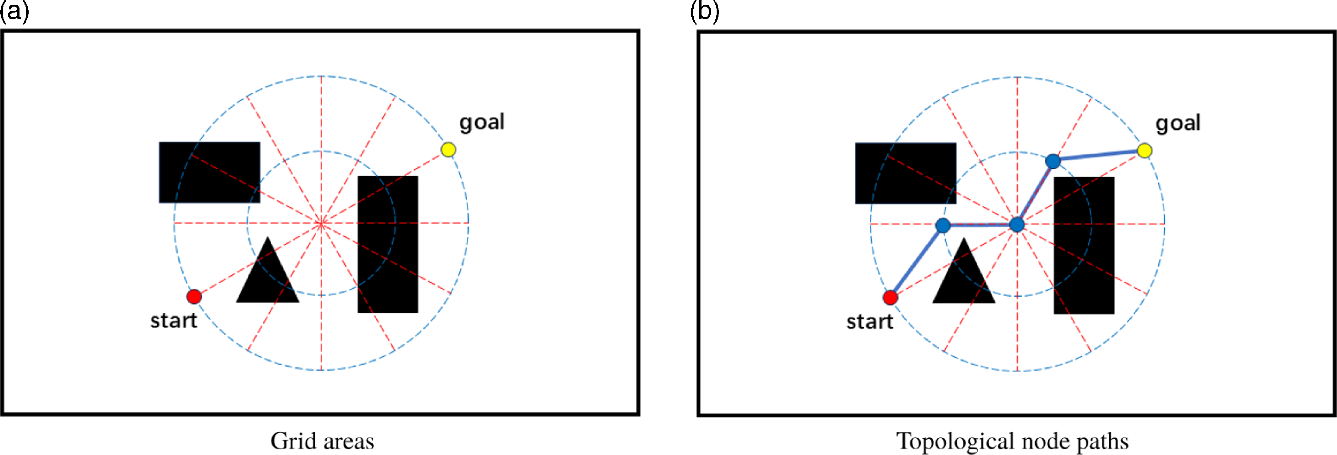
In the query stage of PRM algorithm, the first step is to ascertain whether the start and end points of the path search are in free space. These points are then added as virtual nodes to the constructed roadmap (G (V, E)) and are connected to nearby real nodes (see Figure 2(a)). Next, a graph search algorithm is utilized on the roadmap to obtain a path from the start point to the end point (see Figure 2(b)). The query stage leverages the previously established roadmap (G (V, E)). This approach effectively reduces computational complexity. It also accelerates the search process. Additionally, it enhances the efficiency and reliability of path searching.

Figure 2.

Query stage.

3.3. PRM algorithm analysis

4.1. Concepts of improvement

To address the issues of excessive sampling points, low utilization and long convergence time in PRM algorithms within complex map environments, the research proposes an improved probabilistic roadmap algorithm. This algorithm is based on topological discrimination and lazy collision (TL-PRM). The algorithm has been enhanced in the following two aspects:

Sampling Stage: TL-PRM algorithm introduces topological discrimination, restricted region sampling, and ring-layer linking strategies. Topological discrimination decomposes complex maps into several simpler sub-maps, thereby reducing computational complexity. The restricted region sampling strategy generates random sampling points within ellipses. These ellipses are centered at topological nodes. This approach ensures a higher density of sampling points while reducing their overall number. As a result, it enhances the quality and utilization of sampling points. The ring-layer linking strategy simplifies the construction process of the path graph (G (V, E)). It achieves this by avoiding ineffective connections between closely spaced sampling points. Consequently, this strategy improves the efficiency of the path search.

Query Stage: TL-PRM algorithm introduces lazy collision detection and node reconnection path optimization strategies. The lazy collision detection strategy delays obstacle collision detection until after the path search. This approach avoids extensive collision detection computations in the initial stages. It effectively utilizes sampling points located within obstacles, thereby improving the quality of random sampling points. Additionally, TL-PRM algorithm dynamically adjusts paths by generating extra nodes. This enhancement improves path adaptability and flexibility. The node reconnection strategy prioritizes extra nodes generated outside the convex edges of obstacles. It also removes extra nodes and their paths that do not result in collisions. This process effectively reduces the number of turns in the path, making the generated path better suited to practical driving needs.

4.2. Topological discrimination

In path planning, traditional PRM algorithm typically increases the number of sample points as the map space expands. However, this method also poses challenges: as the map area increases, sample points may deviate from the optimal path or lie within obstacles, making effective utilization difficult. This results in some sample points potentially failing to achieve effective path connections during the path planning process. In contrast, topological path planning methods place greater emphasis on cost for path selection, rather than focusing on the specific content between nodes.

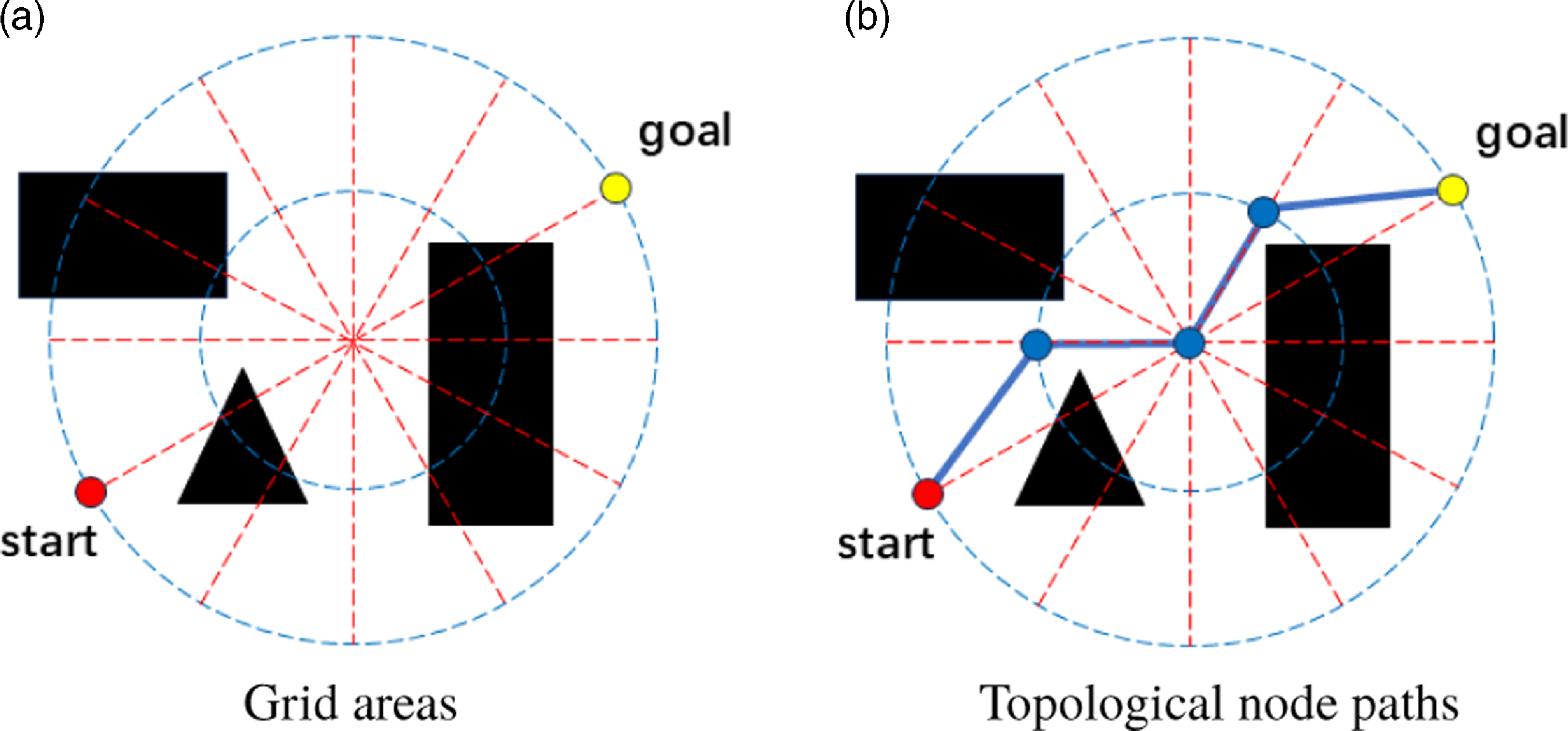
Therefore, this study introduces topological discrimination into the algorithm. It assists decision-making and path planning through the analysis and evaluation of the topological structure of objects or obstacles in the map. Specifically, first, a set of concentric circles $\left ( x_0,y_0 \right)$ is generated with the midpoint of the starting point as the center. Grid areas are created at intervals of thirty degrees (see Figure 3(a)). The parameters are as follows:

(1) \begin{equation} x_{0}=\left (x_{1}+x_{2}\right) / 2 \end{equation}

(2) \begin{equation} y_{0}=\left (y_{1}+y_{2}\right) / 2 \end{equation}

(3) \begin{equation} R_{1}=\sqrt {\left (x_{2}-x_{1}\right)^{2}+\left (y_{2}-y_{1}\right)^{2}} / 2 \end{equation}

(4) \begin{equation} R_{2}=\sqrt {\left (x_{2}-x_{1}\right)^{2}+\left (y_{2}-y_{1}\right)^{2}} / 4 \end{equation}

Subsequently, the area of obstacles within the grid is calculated, which serves as the information for the grid. The formula for calculating the area is as follows:

(5) \begin{equation} S=\int _{\theta _{i}}^{\theta _{i+1}} \int _{r_{k}}^{r_{k+1}} r d r d \theta \end{equation}

Finally, by conducting a path search within this circular grid area, a minimum-cost original path can be quickly generated (see Figure 3(b)). The advantage of this method lies in its combination of the structural properties of the environmental space and cost information, thereby improving the overall efficiency and reliability of path planning.

Figure 3.

Topological discrimination.

4.3. Restricted area sampling

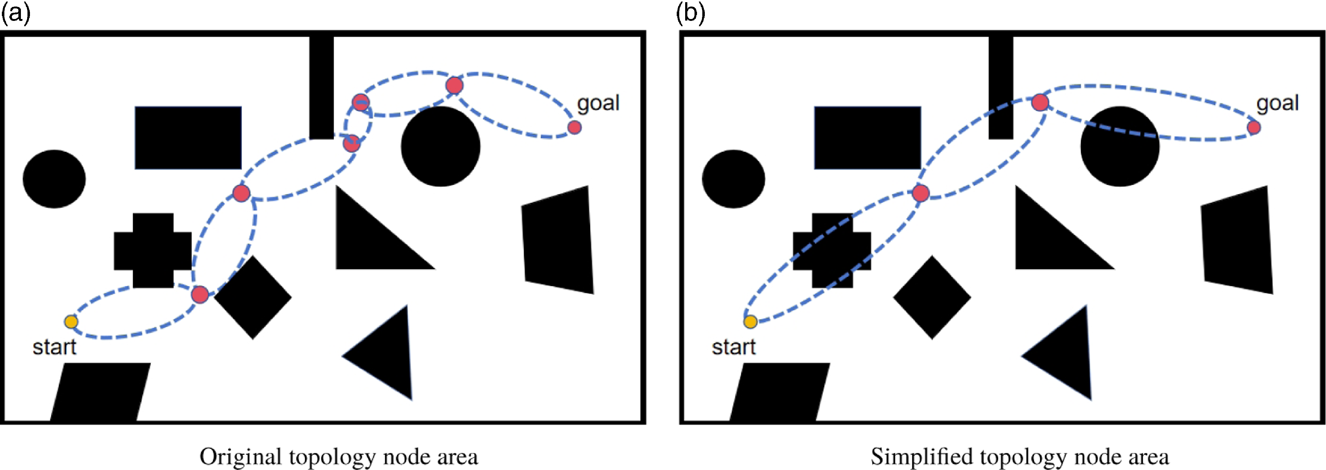
In PRM algorithm, the best path usually appears in the area centered around the starting point and the endpoint. This is especially true near the line connecting the starting point and the target point. In this region, the probability of the shortest path appearing is higher. Based on this characteristic, TL-PRM algorithm proposes a restricted area sampling strategy. This strategy randomly generates sampling points within an elliptical area with topological nodes as endpoints (see Figure 4(a)). This approach reduces the number of sampling points generated and enhances their directionality. As a result, the sampling points become more focused on the vicinity of the best area. The parameters of the ellipse are as follows:

(6) \begin{equation} \frac {(x \cos \theta -y \sin \theta -X)^{2}}{a^{2}}+\frac {(x \sin \theta +y \cos \theta -Y)^{2}}{b_{i}^{2}}=1 \end{equation}

(7) \begin{equation} b_{i}=\frac {a * \tan \varphi }{k} \cdots (k=1,2, \cdots, n) \end{equation}

(8) \begin{equation} \tan \theta =\frac {y_{2}-y_{1}}{x_{2}-x_{1}} \end{equation}

Figure 4.

Restricted area sampling.

TL-PRM algorithm uses a Gaussian distribution as a model to describe the probability of nodes being distributed in space, with the following function:

(9) \begin{equation} P(t)=\frac {1}{2 \pi \sigma ^{2}} e^{-\frac {(t-\mu)^{2}}{2 \sigma ^{2}}} \end{equation}

where $\sigma$ represents the expected value, which can be the average position of the nodes, and $\mu$ represents the standard deviation, indicating the width of the distribution.

Although this restricted sampling area can better focus the sampling points near the best area, it may also lead to an increase in classified areas. This occurs due to an excessive number of topological nodes, which can reduce the algorithm’s convergence speed. To address this issue, TL-PRM algorithm sets a topological node distance threshold L ( $L\gt \frac {a}{3}$ ). This helps to simplify the topological nodes and optimize the restricted sampling area (see Figure 4(b)).

Even though restricted area sampling can effectively reduce the sampling range, decrease redundant nodes, and enhance sampling speed, there are special circumstances to consider. For example, when obstacles cross the elliptical sampling area, the generated path may collide with these obstacles. This can render the roadmap G (V, E) unable to be generated reasonably, leading to a deadlock.

The general solution is to increase the values of the long and short axes of the ellipse. This expansion of the sampling area can result in an increased distribution range of sampling points. To address this issue, the research combines a lazy collision strategy. This strategy can effectively avoid crossing problems while keeping the elliptical sampling area unchanged. As a result, it prevents the distribution range of sampling points from becoming too large.

4.4. Lazy collision

PRM algorithm, after randomly generating sampling points, needs to detect each sampling point to determine if it is inside an obstacle. Any random sampling points generated within obstacles will be discarded in order to filter out sampling points in free space. However, this process can be time-consuming.

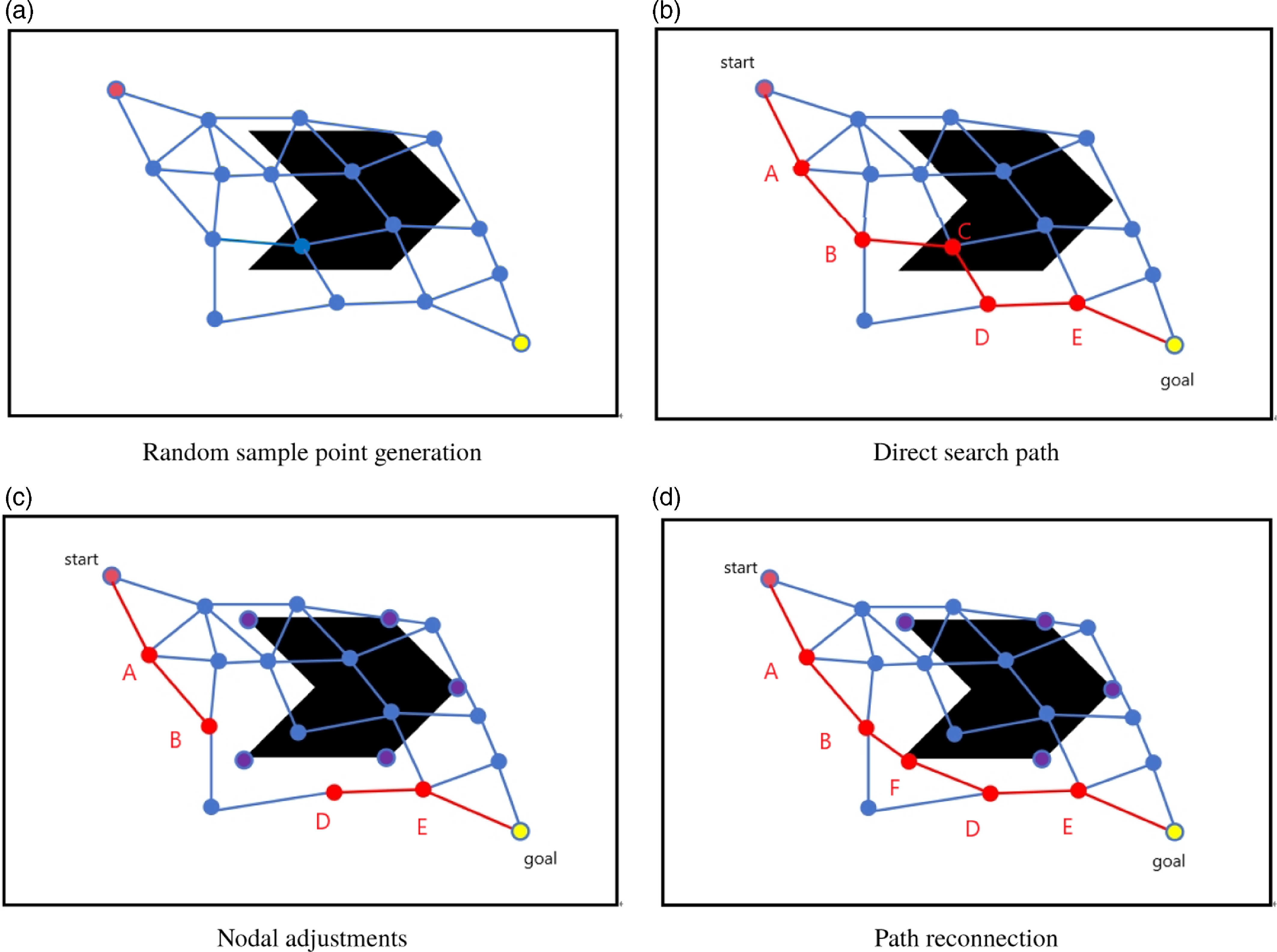
To address this issue, TL-PRM algorithm proposes a lazy collision detection strategy. This approach delays obstacle detection until the path querying phase. It allows for the direct construction of a roadmap after generating the sampling points (see Figure 5(a)).

Figure 5.

Delayed collision detection.

During the path querying phase, if a collision is detected between the path and obstacles (e.g., $\left \{ B-C \right \}$ and $\left \{ C-D \right \}$ in Figure 5(b)), these collision paths will be removed from the graph (G(V, E)). An additional set of sampling points will then be generated on the outer edge of the obstacle (see Figure 5(c)).

The newly generated sampling points will be connected to neighboring nodes and added to the graph. This process will be repeated until the final path no longer collides with obstacles. Eventually, a search algorithm will be used to obtain the final path $\left \{start-A-B-F-D-E-goal\right \}$ (see Figure 5(d)).

Through this method, TL-PRM algorithm can dynamically adjust paths during path planning. This helps to avoid collisions with obstacles and thereby improves the quality and reliability of path planning.

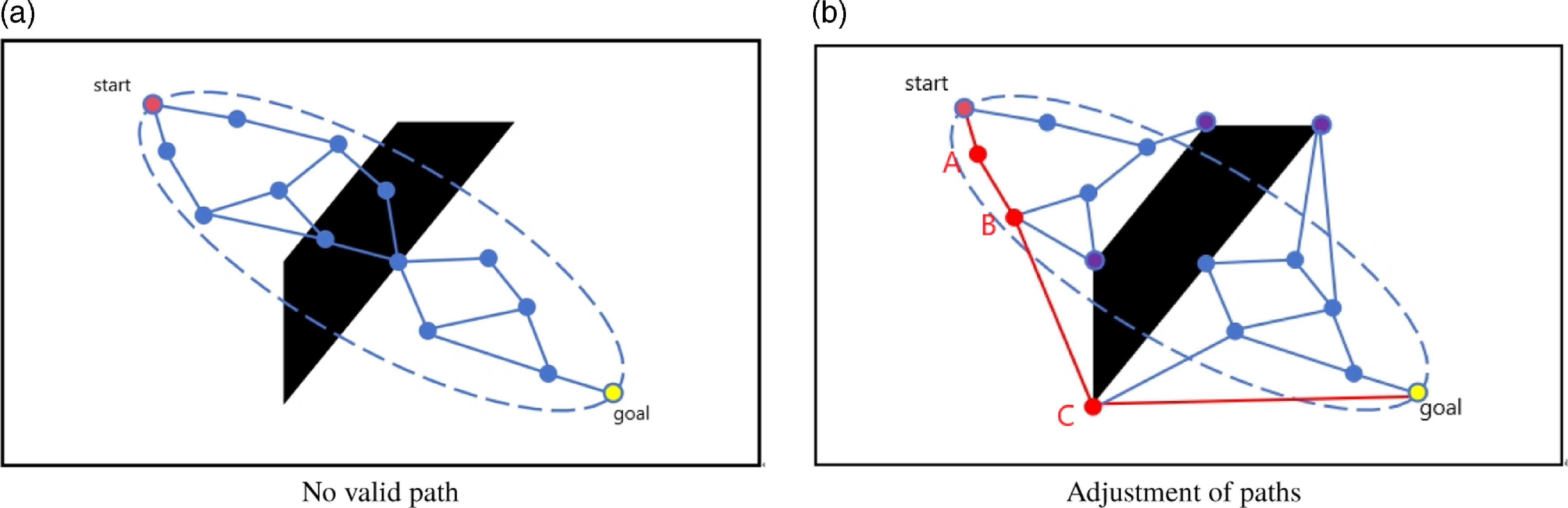
In the event of a special case where obstacles cross the elliptical sampling area (see Figure 6(a)), the lazy collision strategy proposed by TL-PRM algorithm can still effectively solve this problem. According to this strategy, collision paths are first removed. Then, an additional set of sampling points is generated on the outer edge of the obstacle, outside the elliptical sampling area.

Subsequently, the newly generated sampling points are connected with neighboring nodes. Finally, the path $\left \{start-A-B-C-goal\right \}$ is obtained using a search algorithm (see Figure 6(b)).

Figure 6.

Special cases.

TL-PRM algorithm overcomes the performance issues of collision detection in traditional PRM algorithms. It does this by introducing a lazy collision detection strategy. Additionally, it generates extra sampling points when obstacles cross the elliptical sampling area. This allows for dynamic adjustment of paths when necessary during the path planning process. These improvements enhance the efficiency of path planning. They also ensure the accuracy and stability of path planning. As a result, TL-PRM algorithm is more applicable and robust in handling complex environments.

4.5. Ring layer connections

The setting of the connection threshold for sampling points in PRM algorithm directly affects the sampling efficiency and path quality. Typically, a smaller connection threshold can produce more accurate paths, but requires more computational resources. Conversely, a larger connection threshold can reduce computation time, but may lead to less precise paths. In TL-PRM algorithm, when the number of sampling points reaches a certain level, or when additional nodes are generated in special cases, some nodes may be positioned too closely together. The connections between these closely spaced points have little impact on the overall path length, but consume a significant amount of computational resources.

To address this issue, TL-PRM algorithm proposes a layered connection strategy. It sets a set of upper bounds $L_1$ and lower limit $L_2$ connection thresholds to effectively reduce the connection complexity and unnecessary connections. To ensure the success rate of path generation, the connections for the start and end points are not subject to the lower bound. For sampling points other than the start and end points, connections are only made when the distance to other sampling points is less than $L_1$ and greater than $L_2$ . Once these conditions are met, the paths are added to the graph G (V, E). After adding the start and end points, connections are then made with other sampling points within the upper $L_1$ bound distance.

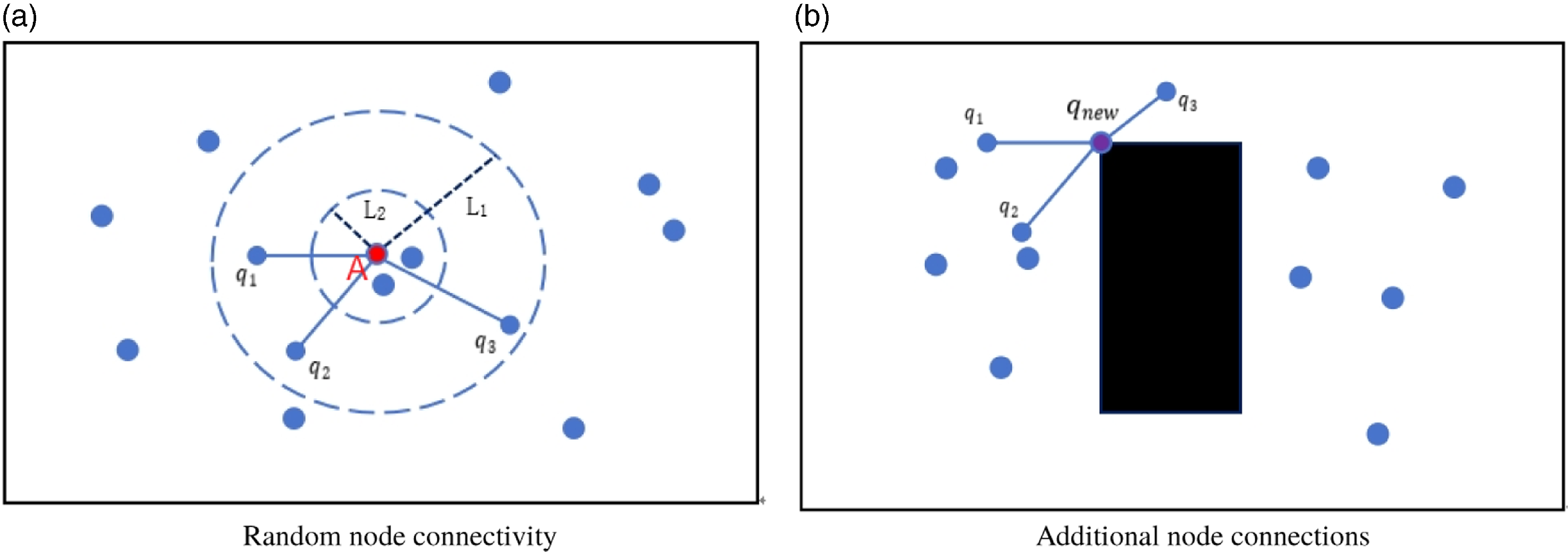
In special cases, such as obstacles crossing the elliptical sampling area, the additional sampling points generated are not subjected to the layered connection evaluation. Instead, they are connected to the three nearest original sampling points. The paths are then added to the graph G (V, E).

Using sampling point A as an example, it will only connect to the points $\left \{ q_{1},q_{2},q_{3} \right \}$ within the layer. These connections will only be made when the distance is less than the upper limit and greater than the lower limit (see Figure 7(a)).

For the additional points generated in special cases, they are connected to the three nearest original sampling points $\left \{ q_{1},q_{2},q_{3} \right \}$ (see Figure 7(b)). This strategy effectively reduces the connection complexity. It eliminates unnecessary connections and ensures the reasonable allocation of computational resources, leading to an improvement in path quality.

Figure 7.

Connection policy.

4.6. Node reconnection

The paths obtained by searching with the TL-PRM algorithm may exhibit an “uneven” and non-smooth appearance. To make the overall path more consistent with actual driving requirements, node reconnection processing is needed. When the algorithm generates additional nodes, the original path will travel along the convex edge of the obstacle. Direct smoothing processing may lead to a wave-like phenomenon at the additional node positions, making the overall path longer. Based on this consideration, TL-PRM algorithm proposes a node reconnection strategy prioritizing the obstacle edge nodes.

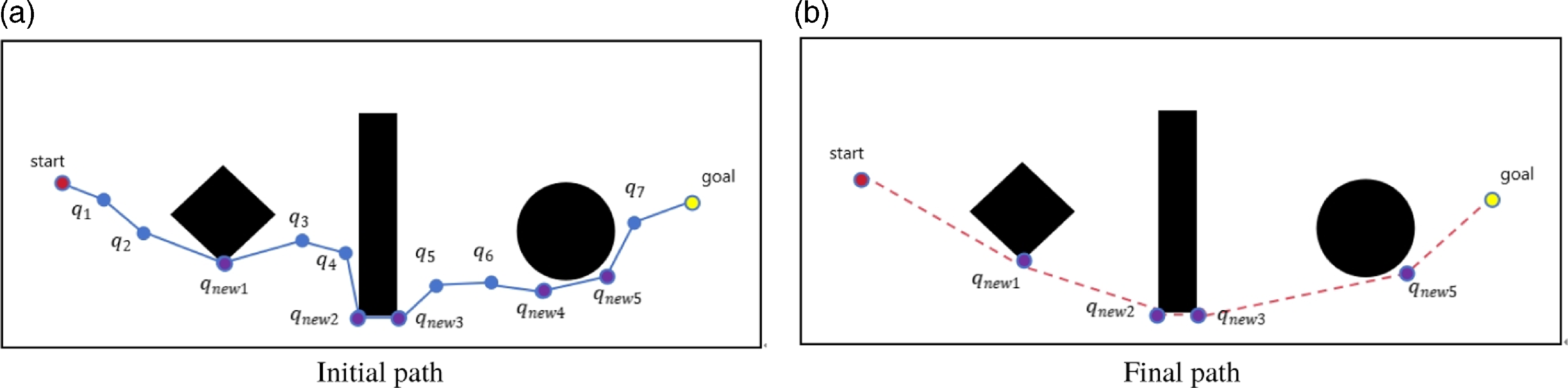
First, TL-PRM algorithm searches for a path and removes the non-path external nodes and connections, with the initial path is $ \{ start-q_1-q_2-q_{new1}-q_3-q_4-q_{new2}-{} q_{new3}-q_5-q_6-q_{new4}-q_{new5}-q_7-goal \}$ (see Figure 8(a)). Here, $q_i$ is sampling nodes, and $q_{new_i}$ is an additional node. Then, collision detection is performed between the path start and the nearest extra node $q_{new1}$ . If there are no obstacles between them, the nodes in between are deleted $\left \{ q_{1},q_{2}\right \}$ . Next, collision detection is performed with the second nearest extra node $q_{new2}$ . If there are obstacles between them, the node $q_{new1}$ is retained and the path start is replaced with that node. Repeat the above process, traversing the start point and additional nodes $\left \{ start,q_{new1},q_{new2},\cdots,q_{new_i},goal \right \}$ and reconnecting the nodes, to obtain the updated path $\left \{ start-q_{new1}-q_{new2}-q_{new3}-q_{new5}-goal \right \}$ (see Figure 8(b)).

Figure 8.

Node reconnection.

4.7. Dynamic environment

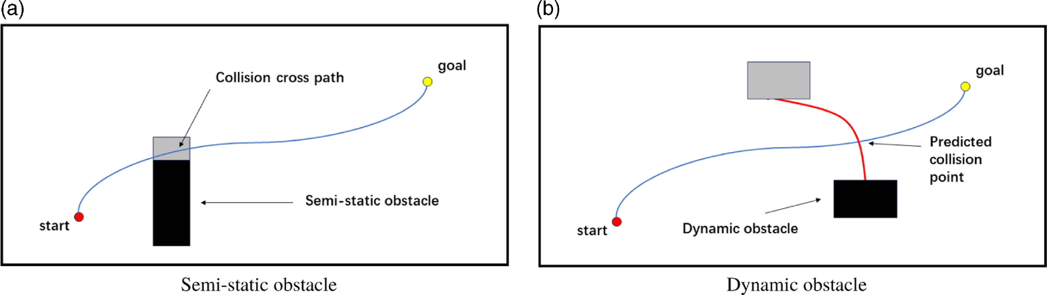
In path planning, uncertainty is a common problem, particularly in dynamic and complex environments. Figure 9(a) illustrates the environmental changes caused by sensor errors, manifested as semi-static obstacles. Figure 9(b) displays obstacles that move in a directed manner.

Figure 9.

Moving obstacle.

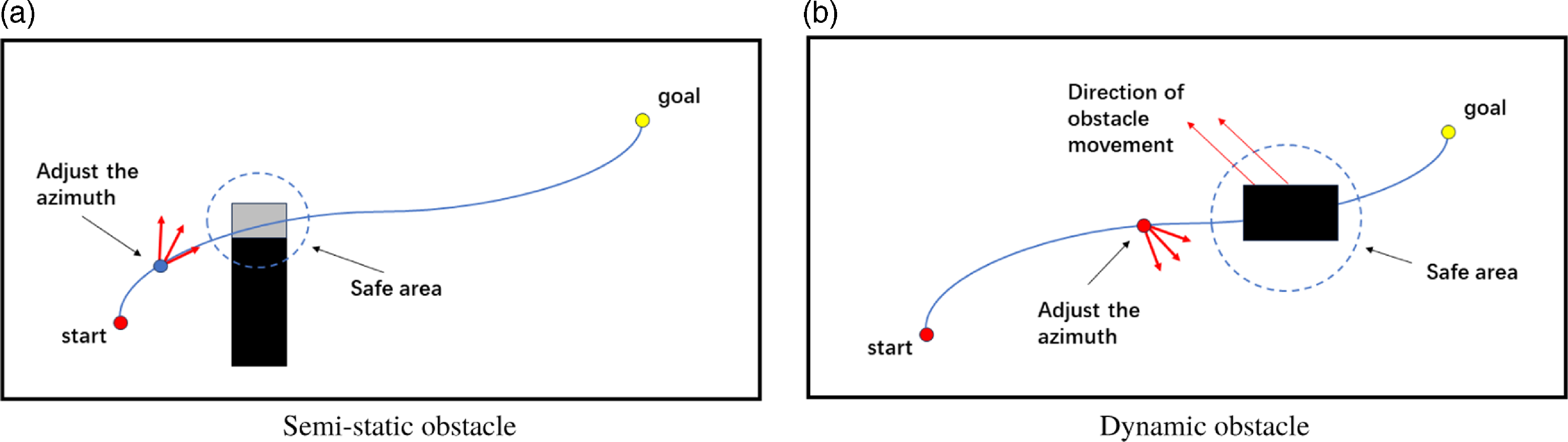
For semi-static obstacles, the mobile robot adjusts its pose angle according to the movement direction of the obstacle (see Figure 10(a)). For moving obstacles, the mobile robot adjusts in the direction opposite to that of the obstacle’s movement (see Figure 10(b)).

Figure 10.

Pose adjustment strategy.

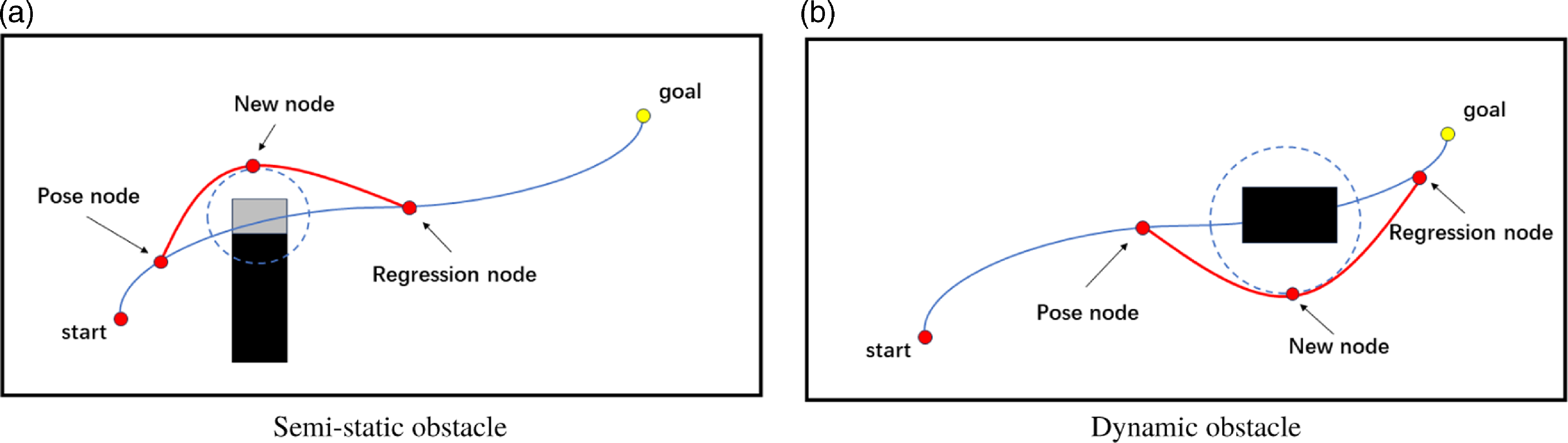
Specifically, since semi-static obstacles will no longer move. It is necessary to find a new node at the farthest point of the obstacle’s safety range after the environmental changes. On the original path, one should select a pose node and a regression node at a distance twice the safety range in order to avoid the obstacle (see Figure 11(a)).

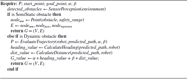
For dynamic obstacles, the trajectory evaluation function is used for dynamic adjustments. The evaluation function is as follows:

(10) \begin{equation} G\left ( v,w \right) =\alpha *heading\left ( v,w \right)+\beta *dist\left ( v,w \right) \end{equation}

where $heading\left ( v,w \right)$ is the azimuth evaluation function. $\alpha$ is taken as a negative value to ensure that the direction angle is adjusted towards the opposite direction of the obstacle’s movement. $dist\left ( v,w \right)$ indicates the distance between the predicted endpoint of the trajectory and the nearest obstacle on the map, thereby reducing the probability of collision between the robot and the obstacle(see Figure 11(b)).

Figure 11.

Avoid the obstacle.

4.8. The overall process TL-PRM algorithm

Inputs: Map information, smart trolley start point, target point, and maximum deflection angle The number of sampling points N, the upper and lower limits of the ring layer connection thresholds $L_1$ , and lower limit $L_2$ and lower limit.

Output: optimal path P, path length L, and path elapsed time T.

Step 1: Initialize algorithm parameters. Generate a circular grid area based on the positions of the starting point and the target point and find the initial path with the lowest cost, forming the topological nodes.

Step 2: Generate the sampling area and construct the roadmap. Create an elliptical sampling area with adjacent topological nodes as endpoints and randomly generate N sampling points within that area. For each sampling point, limit the number of connections based on the upper $L_1$ and lower $L_2$ bounds of the hierarchical connection threshold, thus obtaining the roadmap G (V, E).

Step 3: Path search. Add the starting point and target point to the pathfinding graph, and connect them with other nodes whose distances are less than $L_1$ to update the roadmap. Use Dijkstra’s algorithm to find the shortest path connecting the starting point and the target point in G (V, E).

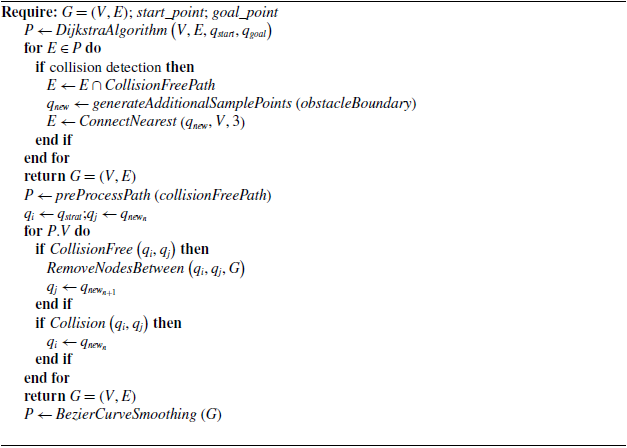
Step 4: Collision detection and path correction. Perform collision detection on the initial path, removing segments that collide with obstacles. Generate a set of additional sampling points at the outer edge of the obstacles and connect them to surrounding nodes. Repeat this process until an effective path that does not intersect with obstacles is obtained.

Step 5: Node reconnection. Remove non-path external nodes and connections, prioritize collision detection between additional nodes, and delete or replace certain nodes in the initial path. Finally, obtain a path that prioritizes the obstacle edges.

Step 6: Dynamic obstacle avoidance. Adjust the forward direction in real-time based on the different categories of dynamic obstacles, using an evaluation function to dynamically optimize the movement direction.

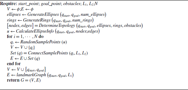
Pseudo-code for TL-PRM algorithm are as follows:

Algorithm 1.

TL-PRM Algorithm Phase I: Sampling Phase

Algorithm 2.

TL-PRM Algorithm Phase II: Query Phase

Algorithm 3.

TL-PRM Algorithm in Dynamic environment

5.1. Algorithm complexity analysis

5.2. Dense map

The first set of tests utilized a dense map with a resolution of 100 $\times$ 100 and a step size of 1 m. This map contained 40 regular obstacles. Additionally, there were multiple paths leading to the target point, which were not obstructed by obstacles. In this context, the algorithm needs to quickly plan a collision-free path. This requires high demands on sampling areas and guidance.

TL-PRM algorithm restricts the sampling area through topological discrimination. The generated topological nodes determine the general direction of the path. This approach effectively reduces the total number of global sampling points. The layering connection strategy simplifies the path graph G (V, E). It enhances both the quality of the path and the efficiency of the algorithm. Furthermore, TL-PRM employs a lazy collision strategy to generate an initial path. It dynamically adjusts the path by generating additional nodes at the edges of obstacles, thus avoiding them. In the path optimization phase, the number of corners is significantly reduced by reconnecting nodes and eliminating intermediate points.

Figure 12.

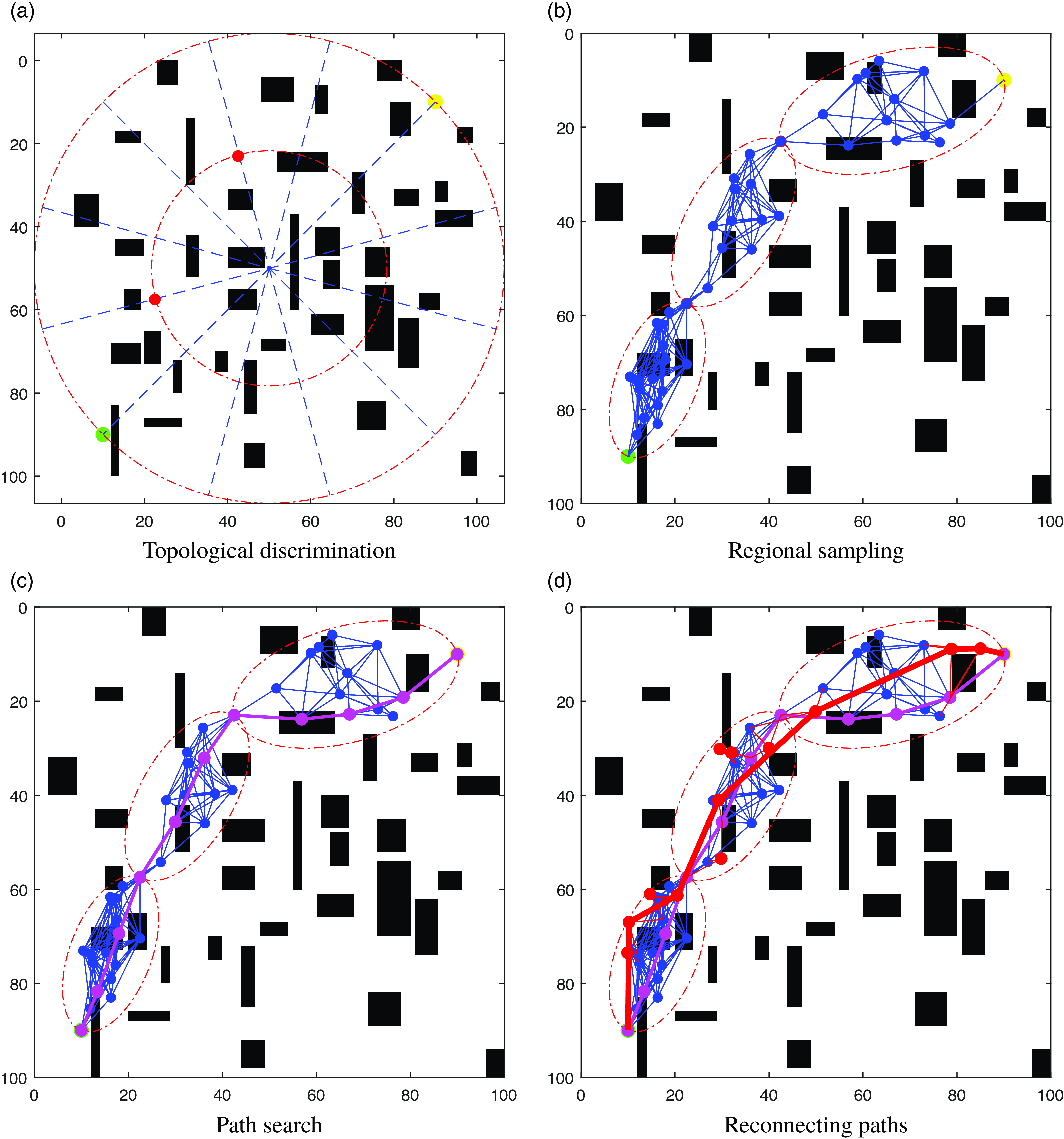
TL-PRM multistage optimization.

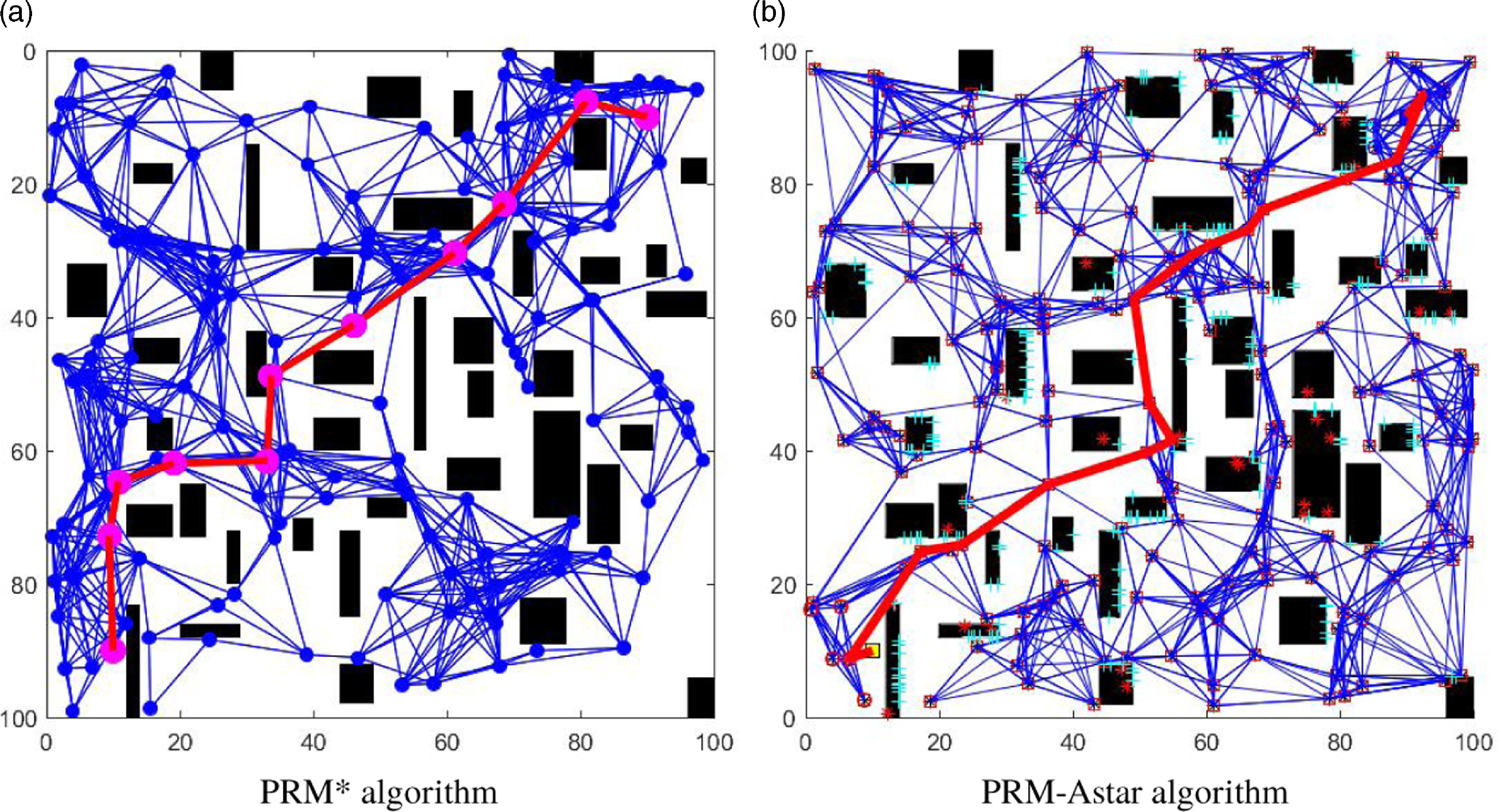
Figure 12 illustrates the detailed process of TL-PRM algorithm. The algorithm first generates a circular grid area, using the start and goal points as endpoints. It seeks the path with the minimum cost to identify the topological nodes (see Figure 12(a)). Next, the algorithm constructs elliptical areas with adjacent topological nodes as endpoints. It generates random sampling points within these areas and connects them via the layering connection strategy (see Figure 12(b)). Subsequently, without performing collision detection, the search algorithm is applied to the generated roadmap to obtain the initial path (see Figure 12(c)).To optimize the path, additional nodes are generated on the outer side of the convex edges of the obstacles. This allows for dynamic adjustments to the path to avoid the obstacles. At the same time, node reconnection is performed to reduce the number of corners (see Figure 12(d)). Figure 13 shows the comparison results ofPRM* and PRM-Astar algorithms.

Figure 13.

Comparison of algorithms.

Simulation results indicate that TL-PRM algorithm requires the fewest sampling points. This demonstrates stronger guidance and results in superior paths. In contrast, PRM* and PRM-Astar algorithms generate sampling points randomly across the entire map. These algorithms lack sufficient guidance, and the quality of each path depends on the distribution of sampling points. PRM algorithm employs bidirectional pathfinding starting at the initial and target points. This yields higher path quality but requires more sampling points. PRM-Astar algorithm uses A* search, which results in fewer sampling points but potentially longer paths.

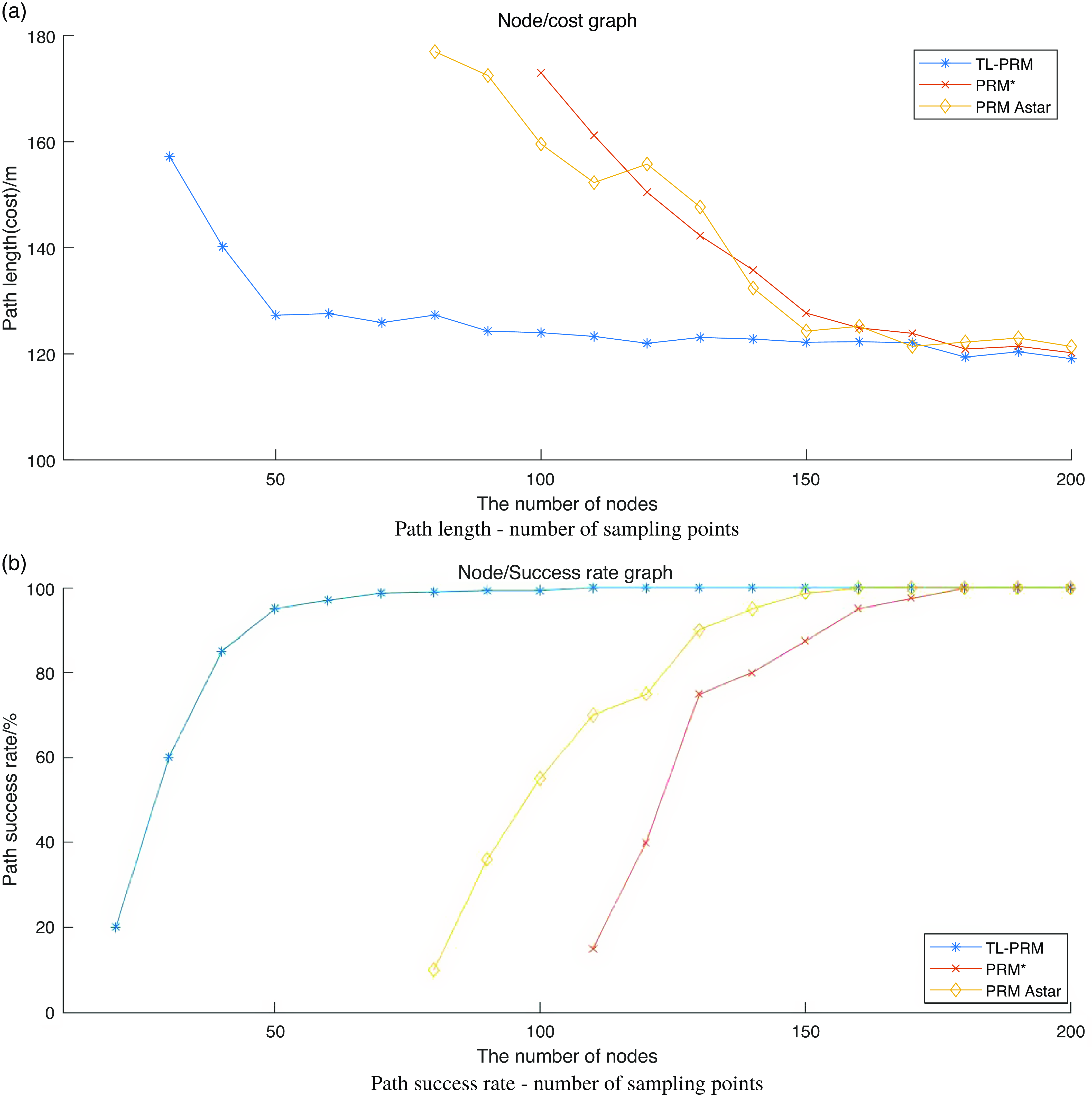
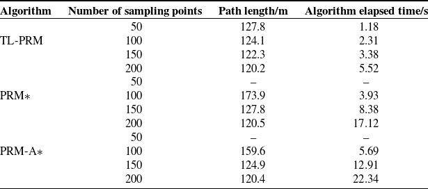
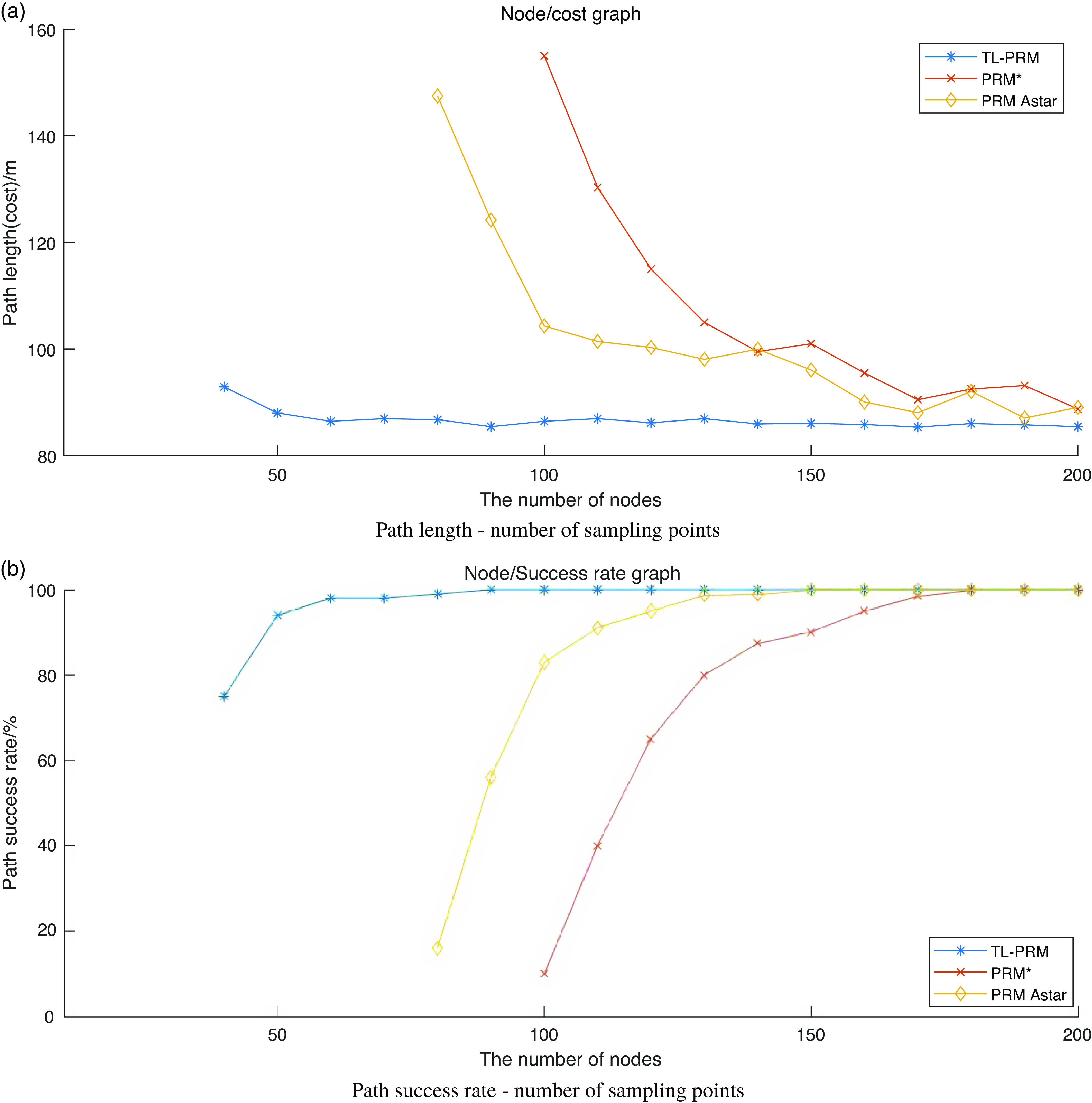
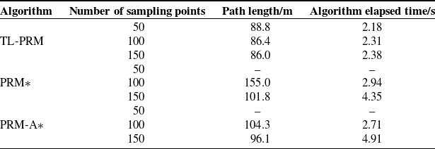
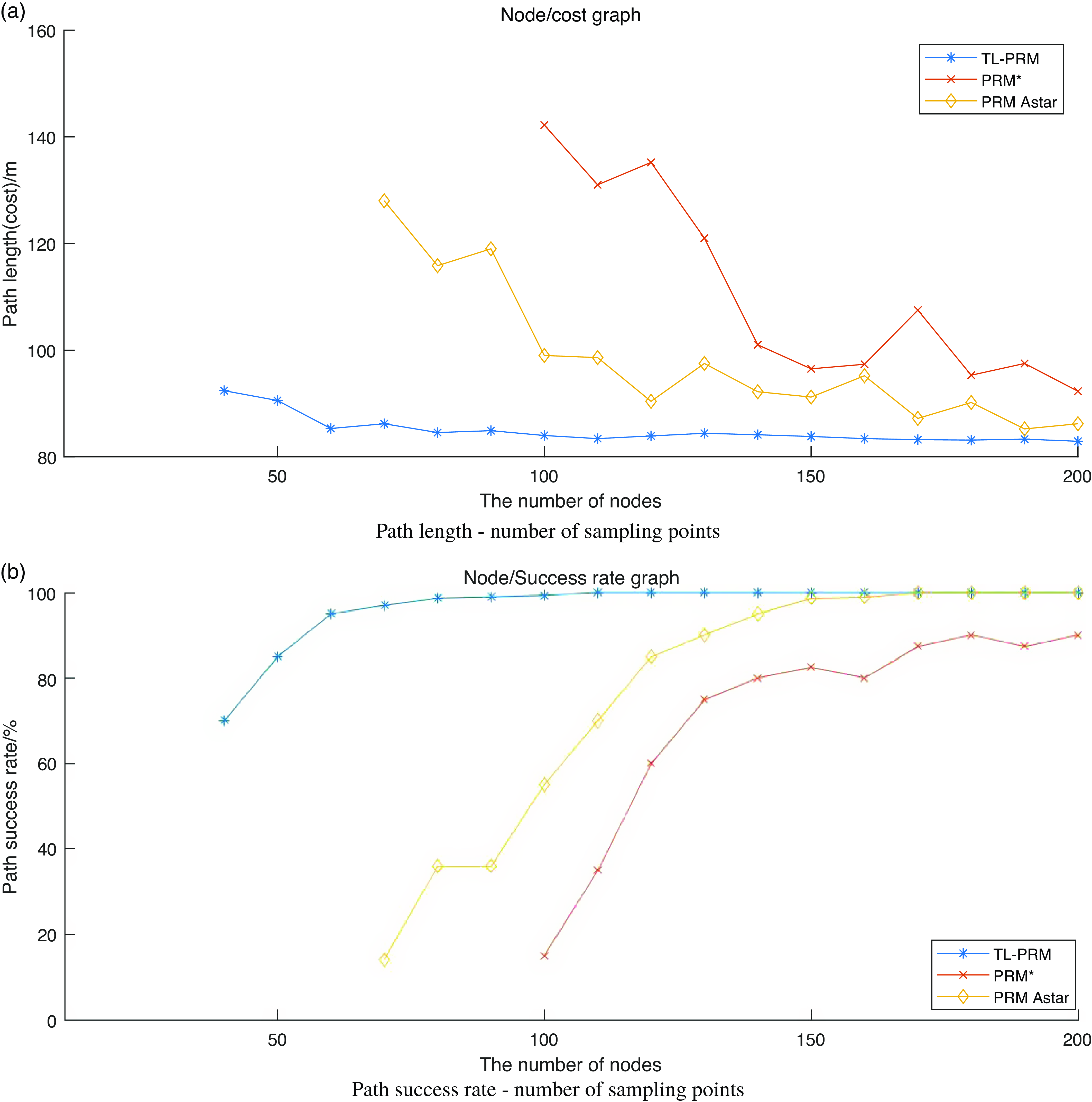
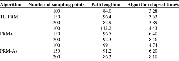
To explore further, testing began with 10 sampling points, increasing by 10 points each time. Based on 50 experiments for each set of node numbers, the path length was taken as the average of the best 5 trials, and the number of successfully generated paths was recorded. Analyzing the number of sampling points for TL-PRM, PRM*, and PRM-Astar algorithms shows the relationship between path length and the number of sampling points in Figure 14(a). The relationship between path success rate and the number of sampling points is shown in Figure 14(b). In addition, a comparative analysis of algorithm convergence time is conducted, with specific data shown in Table I.

Figure 14.

Test results under dense maps.

Table I.

Comparison of algorithms for different sampling points.

Table I presents the path length and execution time of TL-PRM, PRM*, and PRM-Astar algorithms at different numbers of sampling points (50, 100, 150, and 200). When the number of sampling points is small (N = 50), PRM* and PRM-Astar algorithms fail to generate valid paths. Only TL-PRM algorithm can successfully generate paths. With the increase in the number of sampling points, the path length gradually decreases. When the number of sampling points reaches saturation (N = 200), the planned path lengths for the three algorithms are close to 120 m. Additionally, at the same number of sampling points, the execution time of TL-PRM algorithm is significantly lower than that of the other algorithms.

From Figure 14, when the number of sampling points N reaches 160, there is little difference in path length and path success rate among TL-PRM, PRM*, and PRM-Astar algorithms. However, when the number of nodes is small (N $\lt$ 50), TL-PRM algorithm can plan the optimal path. The probability of successfully planning collision-free paths is much higher than that of the comparison algorithms. This indicates that TL-PRM algorithm is significantly more efficient in terms of operational efficiency compared to the other algorithms. It has shorter processing times and faster convergence speeds.

5.3. Circular map

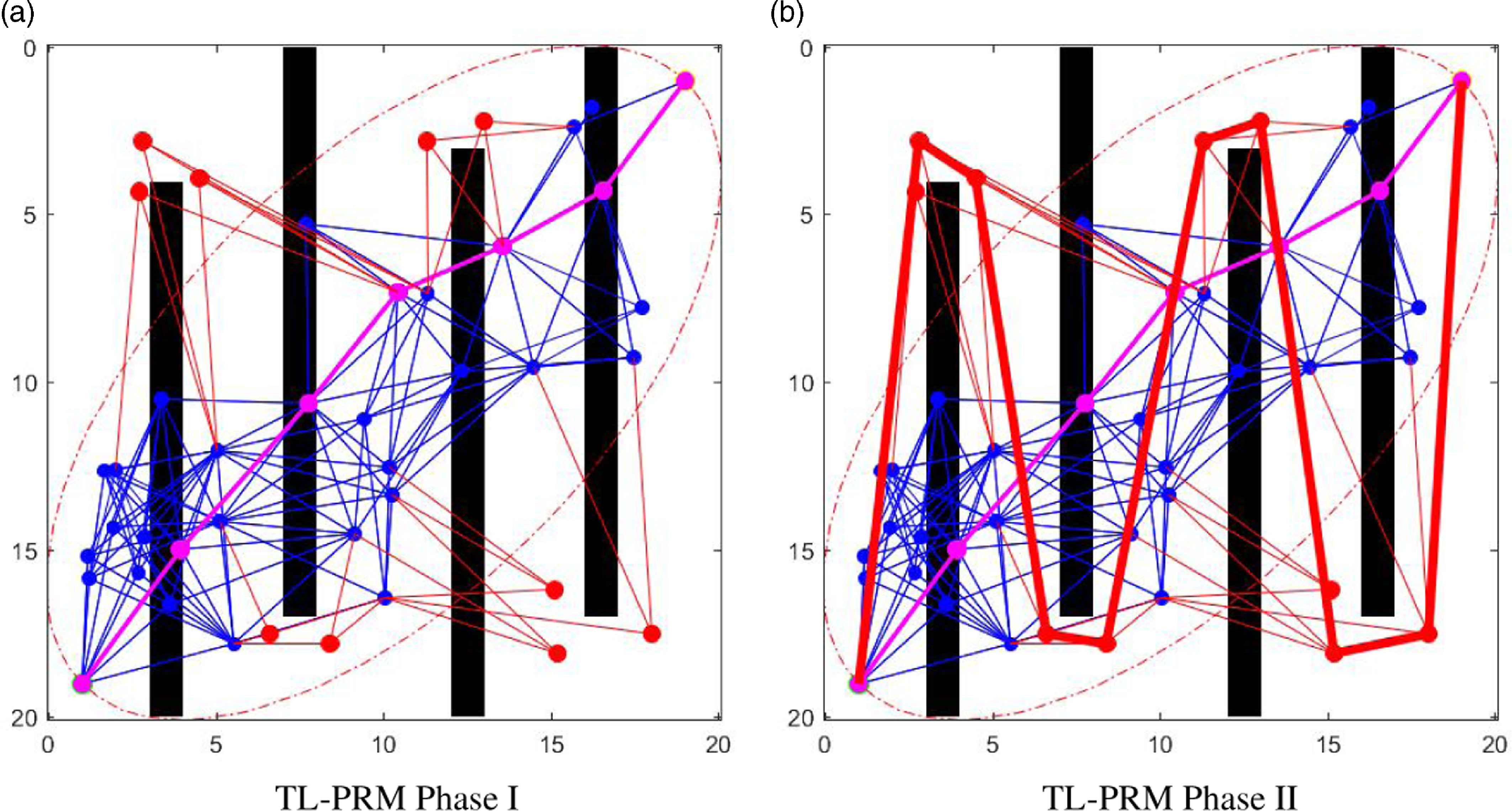
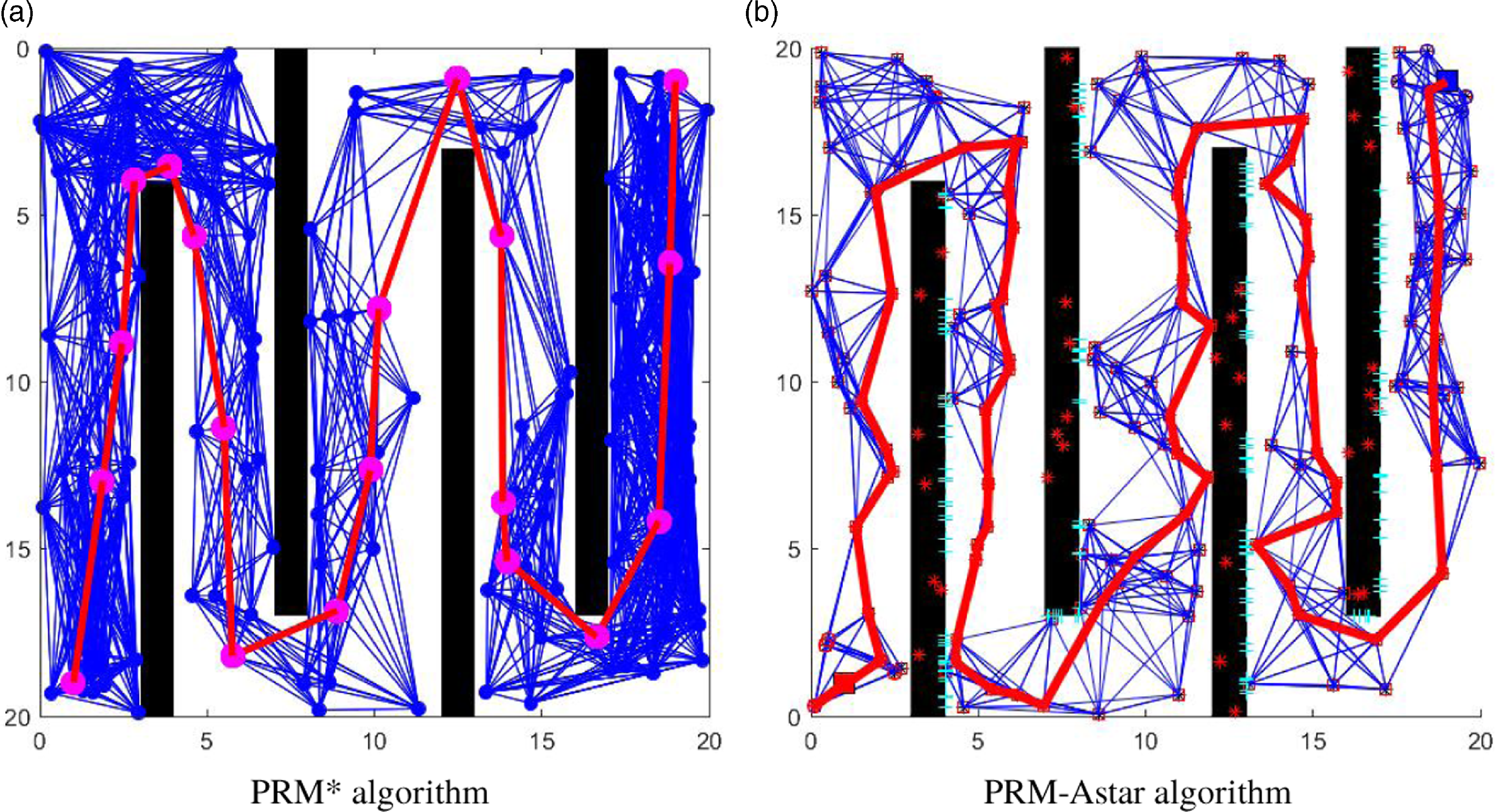
The second set of tests used a meandering map with a resolution of 20 $\times$ 20 and a step size of 1 m. In the [0, 20] region of the map, long obstacle blocks are placed every 3 m. The path is folded in a forward manner, which places high demands on the directionality of the algorithm. Figure 15 and Figure 16 show the simulation results of TL-PRM algorithm compared to PRM* and PRM-Astar algorithms.

Figure 15.

TL-PRM algorithm.

Figure 16.

Algorithm comparison.

Based on the image data, TL-PRM algorithm requires the fewest sampling points. It also has the shortest path length and generates excellent paths. TL-PRM removes non-path points and lines during node reconnection. This significantly reduces the influence of random sampling points on the path. The final path tends to prioritize the selection of edge nodes, resulting in shorter and more stable path lengths. In comparison, the quality of paths generated by PRM* and PRM-Astar algorithms is significantly affected by the distribution of sampling points.

Similar to the first set of experiments, we analyzed different quantities of sampling points. Figure 17(a) shows the relationship between path length and the number of sampling points. Meanwhile, Figure 17(b) shows the relationship between path success rate and the number of sampling points. In addition, a comparative analysis of algorithm convergence time is conducted, with specific data shown in Table II.

Figure 17.

Test results under dense maps.

Table II.

Comparison of algorithms for different sampling points in circular map.

From Table II and Figure 17, when searching for paths in a circumnavigation-type map, the optimal paths generated by TL-PRM algorithm are shorter and more stable than those generated by other algorithms. Additionally, the number of nodes required is also smaller. When the number of nodes reaches a saturation value (N = 170), the path lengths and success rates of TL-PRM, PRM*, and PRM-Astar algorithms are not significantly different. However, when the number of nodes is relatively small (N = 50), the collision-free path length planned by TL-PRM algorithm is 44.2 m shorter than that of the PRM-Astar algorithm. The path success rate is also 80.5% higher than that of PRM* algorithm. This indicates that in circumnavigation-type maps, TL-PRM algorithm can significantly reduce the number of sampling points while maintaining a relatively high path quality.

5.4. Narrow channel map

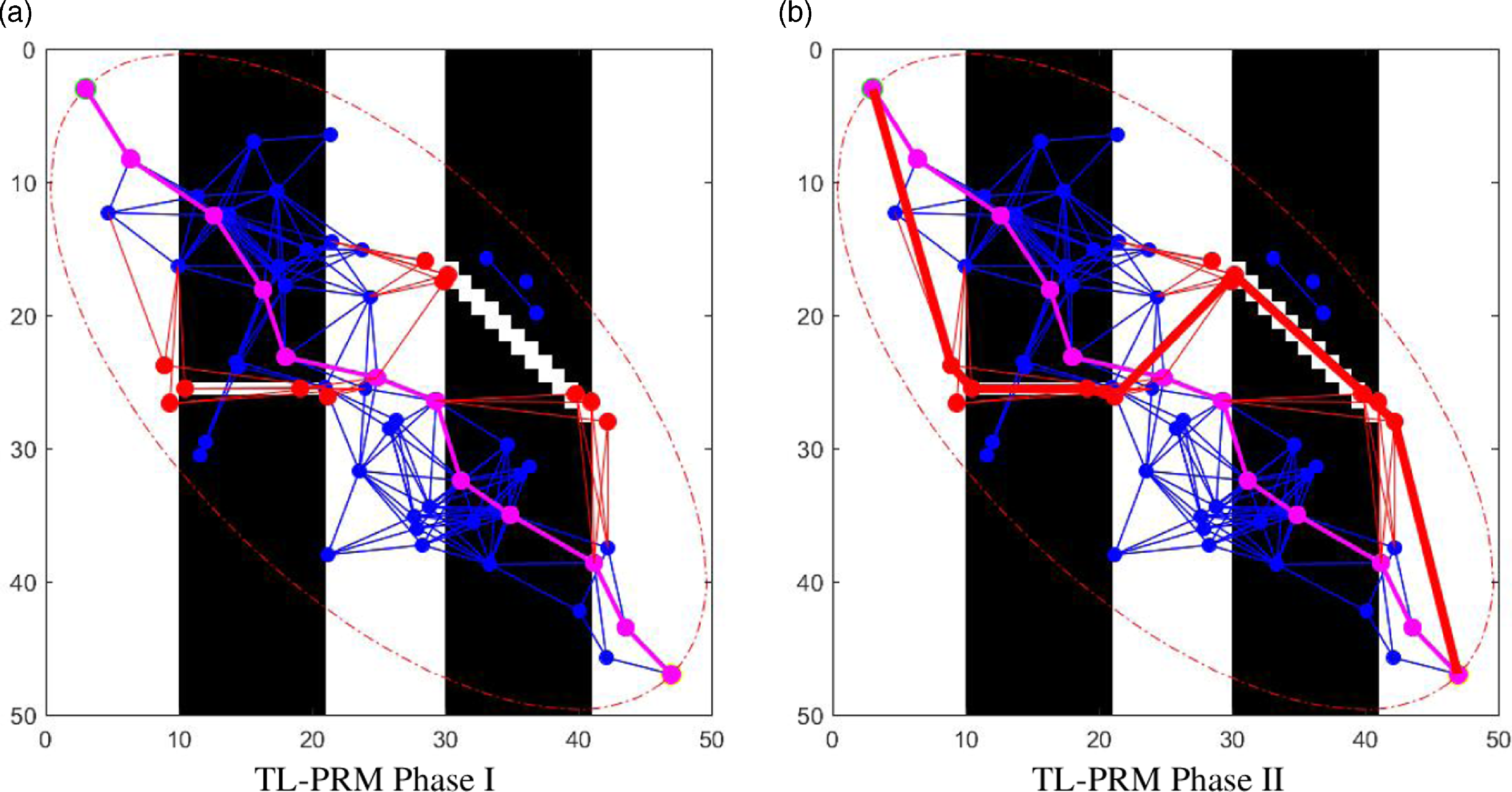
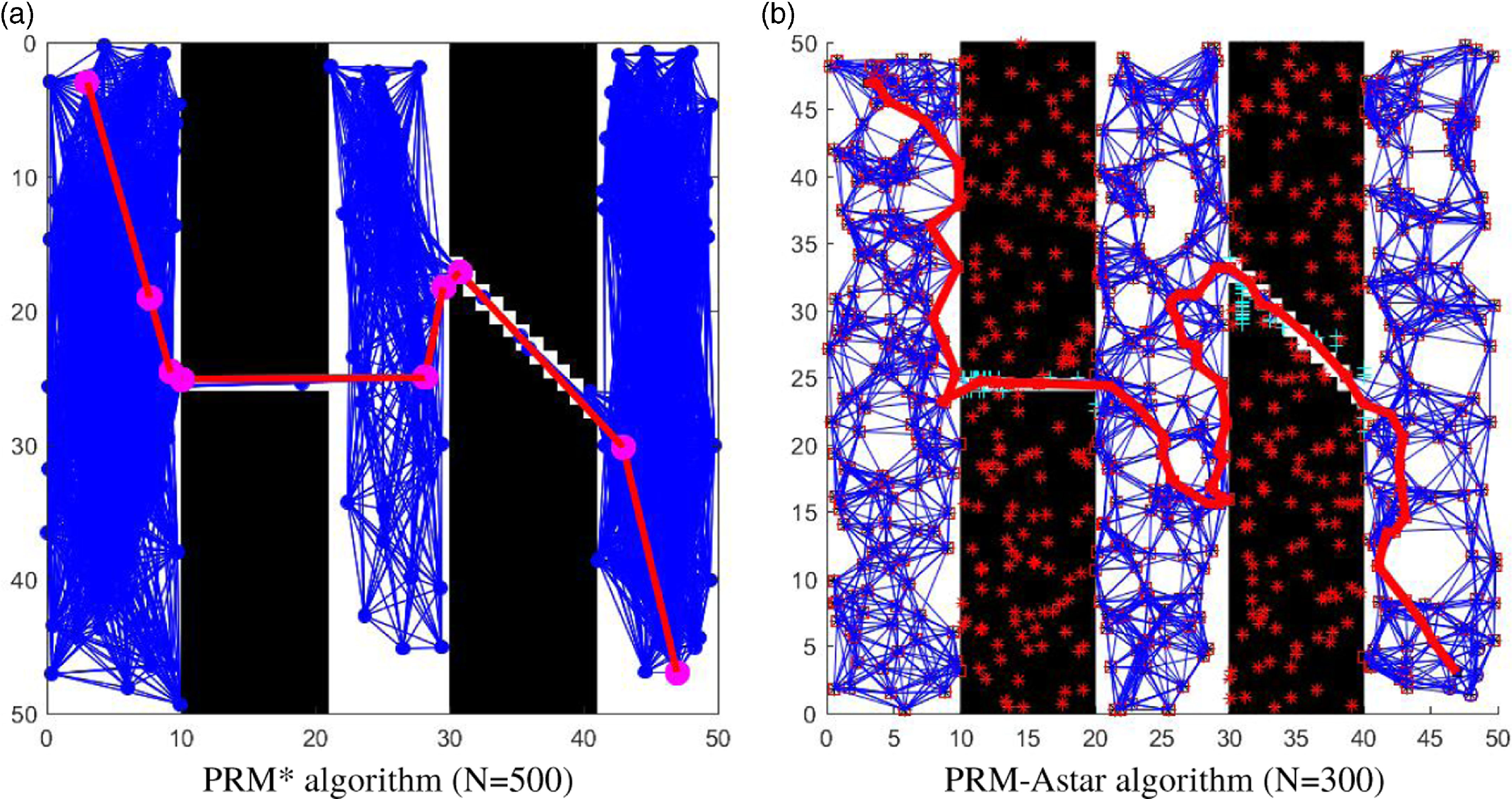
The third set of tests adopted a dual-narrow-passage map with a resolution of 50 $\times$ 50 and a step size of 1 m. This map features a horizontal narrow passage in the [10, 20] region and an oblique narrow passage in the [30, 40] region. Within these narrow passages, there exists only a single unobstructed path. This situation poses a high requirement on the distribution of the sampling points. Figure 18 and Figure 19 show the simulation results of TL-PRM algorithm, as well as those of PRM* and PRM-Astar algorithms.

Figure 18.

TL-PRM algorithm.

Figure 19.

Algorithm comparison.

From the results, TL-PRM algorithm generates significantly fewer sampling points. This is because PRM* and PRM-Astar algorithms are limited by the random generation of sampling points and the step length. A sufficient number of sampling points must be generated within the narrow passage to pass through. In contrast, TL-PRM algorithm can detect obstacles on the initial path and generate additional nodes outside. This capability allows it to overcome the step length limitation and improve sampling quality and guidance. Similar to the first group of experiments, Figure 20 shows the test results and sampling point analysis of the three algorithms in a double-narrow passage map.

Figure 20.

Test results under dual narrow-channel map.

From Figure 20, when searching for the optimal path in the double-narrow passage map, TL-PRM algorithm requires significantly fewer sampling points compared to other algorithms. When the number of nodes is relatively low (N $\lt$ 100), only TL-PRM algorithm has a higher probability of generating a reasonable channel path. When the number of nodes is relatively high (N $\gt$ 100), the convergence speed of TL-PRM algorithm is also faster.

Furthermore, compared to PRM* and PRM-Astar algorithms, when the number of nodes is relatively low (N = 100), the probability of TL-PRM algorithm planning a collision-free path increases to 82.5% and 47.5%. When the number of nodes increases (N = 200), the path orientation becomes more stable. In addition, a comparative analysis of algorithm convergence time is conducted, with specific data shown in Table III.

Table III.

Comparison of algorithms for different sampling points in narrow channel map.

In summary, compared to PRM* and PRM-Astar algorithms, TL-PRM algorithm exhibits superior performance in various types of maps. It generates shorter path lengths, higher success rates, and faster convergence speeds. This fully demonstrates the effectiveness and feasibility of TL-PRM algorithm.

5.5. Dynamic environment

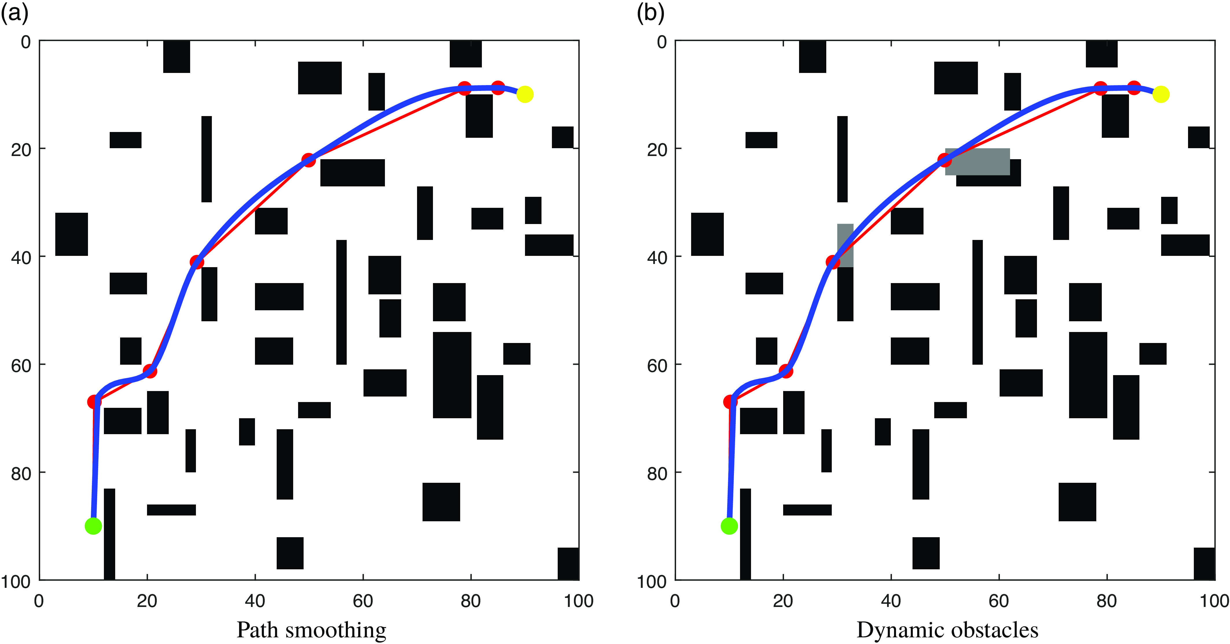
The dynamic environment takes the dense map from Section 5.2 as an example (see Figure 21(a)). In this figure, the red route represents the path searched by TL-PRM algorithm, while the blue route is the path after smoothing. We simulated dynamic obstacles (gray color). Assuming that the obstacle located at the upper-left corner at coordinates (30, 42) is a semi-static obstacle, it will move from (30, 42) to (30, 34) when the vehicle approaches it. Meanwhile, the obstacle at the upper-left corner at coordinates (53, 22) is a dynamic obstacle. It will move from (53, 22) to (50, 20) when the vehicle approaches it (see Figure 21(b)).

Figure 21.

Dynamic environment.

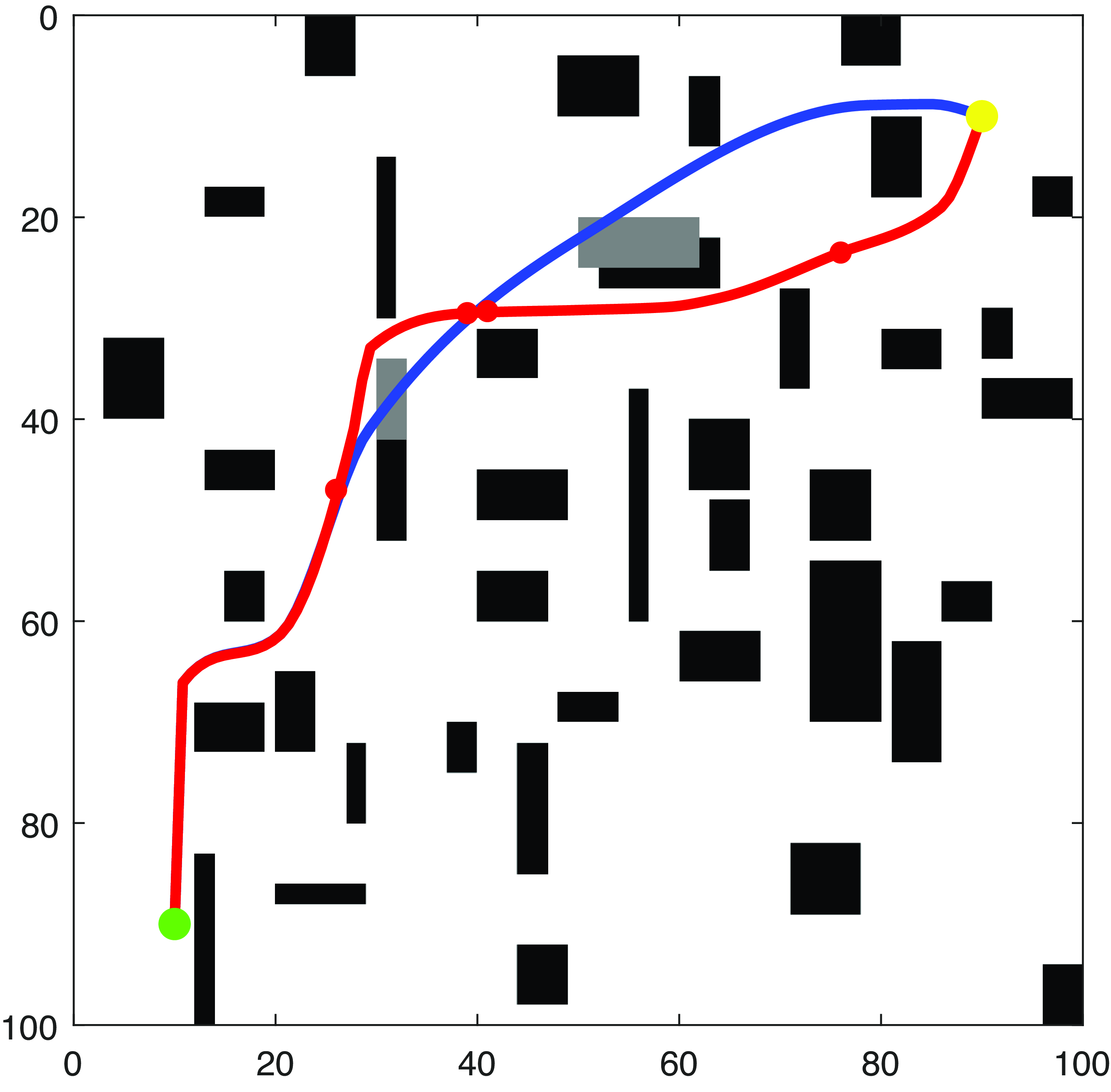
The kinematic model of the robot is as follows: the maximum speed is 5 $m/s$ , the maximum rotational speed is $\pi /6$ $rad/s$ , the acceleration is 1 $m/s^{2}$ , and the smoothed path serves as the original path for navigation. The simulated trajectory is shown in Figure 22.

It can be seen that the motion trajectory is divided into three stages: 1. When no obstacles are detected and the path overlaps with the smooth line, the motion path follows the original route. 2. When a semi-static obstacle is detected and collides with the trajectory, the vehicle adjusts its forward angle. It does this in the direction of the obstacle’s extension. Specifically, it starts from point (26.32, 46.89) and returns to the original route at (39.11, 29.50). 3. When a moving obstacle is detected and collides with the trajectory, the vehicle adjusts its forward angle. It does this in the opposite direction of the obstacle’s movement. Specifically, it starts from point (41.26, 29.36) and returns to the original route at (76.31, 23.45).

Figure 22.

Dynamic obstacle avoidance.