1. INTRODUCTION
Long-endurance high-accuracy autonomous marine navigation is one of the most demanding applications of inertial systems (Titterton and Weston, Reference Titterton and Weston2004). The Rotational Inertial Navigation System (RINS), also known as an indexed Inertial Measurement Unit (IMU), has been widely used in modern ships (Groves, Reference Groves2013).
Normally, the RINS adopts a single-axis or dual-axis rotation scheme to average out the influence of gyro drift and accelerometer bias (Tucker and Levinson, Reference Tucker and Levinson2000; Levinson and Majure, Reference Levinson and Majure1987; Levinson et al., Reference Levinson, Horst and Willcocks1994). Aimed at improving the performance of RINS, corresponding research has been published. Tucker and Levinson (Reference Tucker and Levinson2000) introduced a single-axis rotation scheme including four dwell positions. Yuan et al. (Reference Yuan, Liao and Han2012) analysed the impact of a dual-axis rotation scheme on position accuracy and proposed a 16-phase sequence cycle rotation scheme. In addition, some other important issues, such as calibration method (Zheng et al., Reference Zheng, Han and Zheng2015), environment sensitive error compensation (Cai et al., Reference Cai, Yang, Song, Yin and Liu2016) and position-fix reset technique (Zheng et al., Reference Zheng, Han, Yue and Yuan2016), have been reported.
A single-axis RINS periodically rotates the IMU along its azimuth axis, which only averages out the influence of horizontal gyro drift and accelerometer bias. Since the effect of azimuth gyro drift cannot be averaged out, the single-axis RINS position error builds up with time. In contrast, a dual-axis RINS can average out the gyro drift and accelerometer bias in all directions by periodically rotating the IMU along its azimuth and roll axes (Yuan et al., Reference Yuan, Liao and Han2012). The major error source impacting on position accuracy of a dual-axis RINS is the gyro random walk error which is an inherent characteristic of all laser gyros and cannot be averaged out (Levinson and Majure, Reference Levinson and Majure1987). The random walk error results in a position error approximately proportional to the square root of the navigation time (Lv et al., Reference Lv, Lai, Liu and Nie2014). Hence, based on the precondition of the same gyro accuracy level, the performance of a dual-axis RINS is usually better than a single-axis RINS. For example, the typical position accuracy index for a single-axis RINS is 1 nautical mile (nm)/24 h (Tucker and Levinson, Reference Tucker and Levinson2000). Instead, the reset period of a dual-axis RINS is about 14 days, and the position accuracy index of that can reach 1 nm/14 days (Levinson, et al., Reference Levinson, Horst and Willcocks1994).
To satisfy the long-term high reliability navigation requirements of modern ships, a redundant RINS configuration is usually adopted. Usually two sets of RINS, even three sets of RINS in special applications, are installed (Levinson and San Giovanni, Reference Levinson and San Giovanni1980). Since there is one more gimbal, one more angle readout resolver and other electronic devices in a dual-axis RINS, its size, power, complexity, and cost increase substantially. In contrast, a single-axis RINS has the advantages of higher reliability and moderate cost and is an excellent backup system for higher accuracy dual-axis RINS on modern ships and submarines (Tucker and Levinson, Reference Tucker and Levinson2000). Moreover, the importance of reducing the cost of redundant inertial navigation systems deployed, without loss of high performance, is recognised and is being emphasised to equipment providers (Vajda and Zorn, 2000; Heckman and Baratela, Reference Heckman and Baretela2000; Hays et al., Reference Hays, Schmidt, Wilson, Campbell, Heckman and Gokhale2002). Hence, in a current dual or triple RINS configuration, replacing one dual-axis RINS with another single-axis RINS can not only satisfy the demand of marine INS for high reliability but can also greatly reduce the cost. The novel redundant RINS configuration complements different systems’ advantages, and is a trade-off between position accuracy and reliability as well as cost.
In a dual RINS configuration, the dual-axis RINS is usually designated as the master RINS, and the single-axis RINS only serves as a hot backup system. Once the dual-axis RINS fails, the navigation information is still available through the single-axis RINS. However, since the single-axis RINS cannot average out the residual azimuth gyro drift which is not estimated during the dockside alignment phase, especially with limited alignment time, the position accuracy inevitably decreases. In the case of a triple RINS configuration, only one set of dual-axis RINS is subjectively designated by the operator as the nominally higher accuracy master RINS, while the other dual-axis RINS and the single-axis RINS are used as the hot backup systems to guarantee higher reliability. However, the designated master dual-axis RINS may not be the higher accuracy system unless there are effective online performance evaluation criteria. Given the above facts, two important issues need to be investigated: Firstly, with navigation information fusion in a RINS redundant configuration, the performance of a single-axis RINS can be improved to ensure position accuracy even if the dual-axis RINS fails. Secondly, in a triple RINS configuration, online performance evaluation between the dual-axis RINS needs to be accomplished, so the higher accuracy system can be selected as the master RINS.
In this paper, an augmented error state Kalman filter for redundant RINS is designed, so that the single-axis RINS azimuth gyro drift can be estimated without external benchmark information. Secondly, a position error prediction model of single-axis RINS is devised to predict the position error caused by azimuth gyro drift, whereby the single-axis RINS’ performance can be improved to ensure position accuracy even if the dual-axis RINS fails. Thirdly, without external benchmark information, an online performance evaluation method for dual-axis RINS is proposed in triple RINS configuration.
The rest of the paper is organised as follows. Section 2 designs a novel augmented error state Kalman filter for redundant RINS. Section 3 analyses the observability condition of the above error state dynamic model. A position error prediction model for single-axis RINS is provided in Section 4, while the online performance evaluation method for dual-axis RINS in triple RINS configuration is also given. Section 5 describes semi-physical simulations and experiments including an at-sea test. The conclusions are summarised in Section 6.
2. KALMAN FILTER DESIGN FOR REDUNDANT RINS CONFIGURATION
2.1. Augmented error state dynamic model
Given that RINS has evolved from the strapdown INS, both their error state dynamic models have the same form (Zheng et al., Reference Zheng, Han, Yue and Yuan2016). Taking the position error's difference, the velocity error's difference, and the attitude error's difference between the single-axis RINS 1 and dual-axis RINS k (k=2, 3) as the new error states, the error state dynamic model is given by
 $$\delta \dot{L}_{1k} = {1 \over R_N + h}\delta v_{N_{1k}}, \delta \dot{\lambda}_{1k} = {v_E \cdot \tan L\cdot \sec L \over R_E + h} \delta L_{1k} + {\sec L \over R_E + h}\delta v_{E_{1k}}$$
 $$\delta \dot{{\bf v}}^n_{1k} ={\bf f}^n\times {\bf \phi}^n_{1k} - (2{\bf \omega}^n_{ie} + {\bf \omega}^n_{en}) \times \delta {\bf v}^n_{1k} - (2\delta {\bf \omega}^n_{ie_{1k}} + \delta {\bf \omega}^n_{en_{1k}}) \times {\bf v}^n + {\bf C}^n_{b_1} \delta{\bf f}^{\,b_1}- {\bf C}^n_{b_k}\delta{\bf f}^{\,b_k}$$
 $$\dot{{\bf \phi}}^n_{1k} = -{\bf \omega}^n_{in}\times {\bf \phi}^n_{1k} +\delta{\bf \omega}^n_{in_{1k}}-{\bf C}^n_{b_1}\delta{\bf \omega}^{b_1}_{ib_1}+{\bf C}^n_{b_k}\delta{\bf \omega}^{b_k}_{ib_k}$$
with
 $$\delta L_{1k} = \delta L_1 -\delta L_k,\ \delta\lambda_{1k} =\delta\lambda_1 - \delta \lambda_k,\ \delta{\bf v}_{1k}^n - \delta{\bf v}^n_k,\ {\bf \phi}_{1k}^n={\bf \phi}_1^n-{\bf \phi}_k^n$$
 $$\delta {\bf \omega}^n_{ie_{1k}} = \delta {\bf \omega}^n_{ie_1} - \delta {\bf \omega}^n_{ie_k}=[\matrix{0 &-\omega_{ie}\sin L \cdot \delta L_{1k} &\omega_{ie} \cos L \cdot \delta L_{1k}}]^T$$
 $$\delta {\bf \omega}^n_{en_{1k}} = \delta {\bf \omega}^n_{en_1} - \delta {\bf \omega}^n_{en_k}=\left[\matrix{-{1 \over R_N + h} \delta v_{N_{1k}} &{1 \over R_E + h} \delta v_{E_{1k}} &{\tan L \over R_E + h} \delta v_{E_{1k}} + {v_E\sec^2 L \over R_E+ h} \delta L_{1k}} \right]^T$$
 $$\delta {\bf \omega}^n_{in_{1k}} = \delta {\bf \omega}^n_{ie_{1k}}+ \delta {\bf \omega}^n_{en_{1k}},\ {\bf \omega}^n_{in}={\bf \omega}^n_{ie}+{\bf \omega}^n_{en}$$
 $$\delta {\bf \omega}^{b_1}_{ib_1} = {\bf \varepsilon}_1 + {\bf w}_{\varepsilon_{1}},\ \delta {\bf \omega}^{b_k}_{ib_k} = {\bf \varepsilon}_k + {\bf w}_{\varepsilon_k},\ \delta {\bf f}^{\,b_1}={\bf \nabla}_1 + {\bf w}_{\nabla_1},\ \delta {\bf f}^{\,b_k}={\bf \nabla}_k + {\bf w}_{\nabla_k}$$
where δ L 1k denotes the difference between the single-axis RINS 1 latitude error δ L 1 and the dual-axis RINS k (k=2, 3) latitude error δ L k, δλ1 denotes the difference between the single-axis RINS 1 longitude error δλ1 and the dual-axis RINS k longitude error δλk. δ v1kn denotes the difference between the single-axis RINS 1 velocity error δ v1n and the dual-axis RINS k velocity error δvkn.  ${\bf \phi}^{n}_{1k}$ denotes the difference between the single-axis RINS 1 attitude error
 ${\bf \phi}^{n}_{1}$ and the dual-axis RINS k attitude error
 ${\bf \phi}^{n}_{k}$;
 ${\bf \omega}^{n}_{ie}$ is the earth rotation rate in the n frame (East-North-Up),
 ${\bf \omega}^{n}_{en}$ is the transport rate,
 ${\bf \omega}^{n}_{in}$ is the angular rate of the navigation frame relative to the inertial frame i; similarly,
 $\delta {\bf \omega}^{n}_{ie_{1k}}$ denotes the earth rotation rate error's difference,
 $\delta {\bf \omega}^{n}_{en_{1k}}$ denotes the transport rate error's difference and
 $\delta {\bf \omega}^{n}_{in_{1k}}$ denotes the navigation frame angular rate error's difference.
 $\delta {\bf \omega}^{b_{1}}_{ib_{1}}$ and
 $\delta {\bf \omega}^{b_{k}}_{ib_{k}}$ are the gyro triad error vectors modelled as the sum of constant drift and white noise and
 $\delta {\bf f}^{\,b_{1}}$ and
 $\delta {\bf f}^{\,b_{k}}$ are the accelerometer triad error vectors modelled as the sum of constant bias and white noise. fn and vn are the specific force and the velocity vector expressed in the navigation frame. Since each RINS is installed adjacent to each other, with relative distance usually less than 1 m, the latitude, the velocity, and the specific force approximately reflect the information from the same point.
In addition, further taking the gyro triad drift vectors of RINS 1 and RINS k, that is,  ${\bf \varepsilon}_{1}$ and
 ${\bf \varepsilon}_{k}$, as well as the accelerometer triad bias vectors of RINS 1 and RINS k, that is,
 ${\bf \nabla}_{1}$, and
 ${\bf \nabla}_{k}$, as the augmented error states, the corresponding error state dynamic model is given by
 $$\dot{\bf \varepsilon}_1 = {\bf 0}, \dot{\bf \varepsilon}_k = {\bf 0}, \dot{\bf \nabla}_1 = {\bf 0}, \dot{\bf \nabla}_k = {\bf 0}$$
The augmented error state vector of the redundant RINS configuration is given by
 $${\bf x}(t) = [\delta L_{1k}, \delta \lambda_{1k}, \delta v_{E_{1k}}, \delta v_{N_{1k}},\phi_{E_{1k}},\phi_{N_{1k}}, \phi_{U_{1k}}, \varepsilon_{1x},\varepsilon_{1y},\varepsilon_{1z},\varepsilon_{kx},\varepsilon_{ky},\varepsilon_{kz},\nabla_{1x},\nabla_{1y},\nabla_{kx},\nabla_{ky}]^T$$
The process noise vector can be written as:
 $${\bf w}(t) = [w_{\varepsilon_{1x}}, w_{\varepsilon_{1y}}, w_{\varepsilon_{1z}}, w_{\varepsilon_{kx}}, w_{\varepsilon_{ky}}, w_{\varepsilon_{kz}}, w_{\nabla_{1x}}, w_{\nabla_{1y}}, w_{\nabla_{kx}}, w_{\nabla_{ky}}]^{T}$$
The error states of the vertical channel are ignored due to their weak coupling with horizontal channels (Bar-Itzhack and Berman, Reference Bar-Itzhack and Berman1988). The augmented error state dynamic model is
 $$\dot{{\bf x}}(t) = {\bf F}(t){\bf x}(t) + {\bf G}(t){\bf w}(t)$$
The components of system matrix F(t) and noise matrix G(t) are listed in the Appendix.
2.2. Measurement model
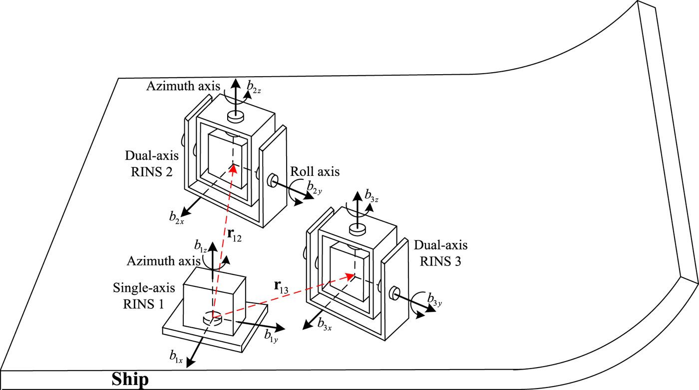
Figure 1 depicts a triple RINS configuration. With the dual-axis RINS 3 removed, the illustration also applies to the dual RINS configuration. The navigation information output including position and velocity from single-axis RINS 1 and dual-axis RINS k(k=2, 3) satisfies the following constraints
Illustration of the redundant RINS configuration.

 $$\tilde{\bf r}_{1}^{n} = {\bf r}^{n} + \delta {\bf r}_{1}^{n}, \tilde{\bf r}_{k}^{n} = {\bf r}^{n} + {\bf r}_{1k}^{n} + \delta {\bf r}_{k}^{n}$$
 $$\tilde{\bf v}_{1}^{n} = {\bf v}^{n} + \delta {\bf v}_{1}^{n}, \tilde{\bf v}_{k}^{n} = {\bf v}^{n} + {\bf \omega}_{b_{1} b_{k}}^{n} \times {\bf r}_{1k}^{n} + \delta {\bf v}_{k}^{n}$$
where  $\tilde{{\bf r}}_{1}^{n}$ and
 $\tilde{{\bf r}}_{k}^{n}$ respectively denote the position output of the single-axis RINS 1 and dual-axis RINS k, δr1n and δrkn denote their position errors, rn denotes the true position, r1k denotes the lever-arm between the single-axis RINS 1 and dual-axis RINS k;
 $\tilde{\bf v}_{1}^{n}$ and
 $\tilde{\bf v}_{k}^{n}$ denote the velocity output of the single-axis RINS 1 and dual-axis RINS k.
 ${\bf \omega}_{b_{1}b_{k}}^{n}$ denotes the relative angular rate between the IMU frame b 1 and b k.
Since the lever-arm is usually less than 1 m and can be accurately calibrated in advance, its influence can be ignored. Respectively subtracting the second equation from the first equation in Equations (13) and (14), and ignoring the lever-arm effect yields
 $$\delta {\bf r}_{1k}^{n} = \delta {\bf r}_{1}^{n} - \delta {\bf r}_{k}^{n} = \tilde{{\bf r}}_{1}^{n} - \tilde{{\bf r}}_{k}^{n}, \delta {\bf v}_{1k}^{n} = \delta {\bf v}_{1}^{n} - \delta {\bf v}_{k}^{n} = \tilde{\bf v}_{1}^{n} - \tilde{\bf v}_{k}^{n}$$
The corresponding components form is given by
 $$\delta L_{1k} = \tilde{L}_{1} - \tilde{L}_{k}, \delta \lambda_{1k} = \tilde{\lambda}_{1} - \tilde{\lambda}_{k}, \delta v_{E_{1k}} = \tilde{v}_{E_{1}} - \tilde{v}_{E_{k}}, \delta v_{N_{1k}} = \tilde{v}_{N_{1}} - \tilde{v}_{N_{k}}$$
The measurement model of the augmented error states is given by
 $${\bf z}(t) = {\bf H}(t){\bf x}(t) + {\bi v}(t)$$
with
 $${\bf z}(t) = [\matrix{\delta L_{1k} &\delta \lambda_{1k} &\delta v_{E_{1k}} &\delta v_{N_{1k}}}]^T, \quad {\bf H}(t) = \left[\matrix{{\bf I}_{2} &0_{2\times 2} &0_{2\times 13} \cr 0_{2\times 2} &{\bf I}_{2} &0_{2\times 13}} \right]$$
where v(t) denotes the measurement noise vector.
3. OBSERVABILITY CONDITION
Partitioning the augmented error state  ${\bf x}(t)$ into two parts yields
 $$\eqalign{{\bf x}(t)&=\left[\matrix{{\bf x}_{1}^{T}(t) &{\bf x}_{2}^{T}(t)} \right]^{T} \cr {\bf x}_{1}(t)&=[ \delta L_{1k}, \delta \lambda_{1k}, \delta v_{E_{1k}}, \delta v_{N_{1k}}]^{T}, \cr {\bf x}_{2}(t) &= [\phi_{E_{1k}},\phi_{N_{1k}}, \phi_{U_{1k}}, \varepsilon_{1x}, \varepsilon_{1y}, \varepsilon_{1z}, \varepsilon_{kx}, \varepsilon_{ky}, \varepsilon_{kz}, \nabla_{1x}, \nabla_{1y}, \nabla_{kx}, \nabla_{ky}]^T}$$
The system described by Equations (12) and (17) can be rewritten as follows (see Appendix)
 $$\left\{\matrix{\left[\matrix{\dot{\bf x}_1(t)\cr \dot{\bf x}_2(t)} \right] = \left[\matrix{{\bf F}_{11}(t) &{\bf F}_{12}(t)\cr \hdashline \cr {\bf F}_{21}(t) &{\bf F}_{22}(t)}\right] \left[\matrix{{\bf x}_1(t)\cr {\bf x}_2(t)} \right] + {\bf G}(t) {\bf w}(t)\cr {\bf z}(t) = {\bf H}(t){\bf x}(t) + {\bi v}(t) = {\bf x}_{1}(t) + {\bi v}(t)} \right.$$
The deterministic observability ignores the influence of noise (Wu et al., Reference Wu, Zh, Wu, Hu and Hu2012). Since x1(t) is directly observable from the measurement z(t), the observability condition of the system described by Equation (20) is the same as the following reduced-order dynamic system (Rhee et al., Reference Rhee, Abdel-Hafez and Speyer2004; Zheng et al., Reference Zheng, Han and Zheng2015)
 $$\left\{\matrix{\dot{\bf x}_{2}(t) = {\bf F}_{22}(t){\bf x}_{2}(t) + {\bf F}_{21}(t) {\bf z}(t) \hfill \cr {\bf y}(t) = {\bf F}_{12}(t){\bf x}_{2}(t) \hfill} \right.$$
For large ships, with lower speeds and less manoeuvring,  ${\bf \omega}_{ie}^{n}\gg {\bf \omega}_{en}^{n}\approx {\bf 0}$ and
 ${\bf f}^{\,n}\approx-{\bf g}^{n}$ apply to most cases (Zheng et al., Reference Zheng, Han, Yue and Yuan2016). According to Equation (A4), the system and measurement matrices of Equation (21) can be approximately simplified as follows
 $${\bf A}(t)\triangleq {\bf F}_{22}(t) = \left[\matrix{-[{\bf \omega}_{ie}^{n} \times ] &-{\bf C}_{b_{1}}^{n} &{\bf C}_{b_{k}}^{n} &0_{3\times 4} \cr \hdashline \cr &0_{10 \times 13}} \right], {\bf C}(t) \triangleq{\bf F}_{12}(t) = \left[\matrix{0_{2\times 3} & 0_{2\times 6} & 0_{2\times 4}\cr {\bf F}_{5} & 0_{2\times 6} &{\bf F}_{6}}\right]$$
with
 $${\bf F}_{5} = \left[\matrix{0 & -g & 0 \cr g & 0 & 0} \right], {\bf F}_{6} = \left[\overline{\bf C}_{b_{1}}^{n} - \overline{\bf C}_{b_{k}}^{n} \right] $$
The stripped observability matrix can be used to analyse the observability of Equation (21) (Goshen-Meskin and Bar-Itzhack, Reference Goshen-Meskin and Bar-Itzhack1992), and is given by
 $${\bf O}(m) = \left[\matrix{{\bf O}_{1}^{T} &{\bf O}_{2}^{T} &\cdots &{\bf O}_{m}^{T}} \right]^{T}$$
with
 $${\bf O}_{j} = \left[\matrix{{\bf C}^{T} &({\bf CA})^{T} &({\bf CA}^{2})^{T} &\cdots &({\bf CA}^{12})^{T}} \right]^{T}; j = 1,2, \ldots, m$$
where the state number of the reduced-order dynamic system is 13, and m is the segments.
Substituting Equation (22) into Equation (25), the general form of CAi (i=1,2,···,12) is
 $${\bf CA}^{i} = \left[\matrix{&0_{2\times 13}\cr \hdashline \cr {\bf F}_{5}[(-1)^{i}[{\bf \omega}^n_{ie}\times]^i &(-1)^i[{\bf \omega}^n_{ie}\times]^{i-1}{\bf C}^n_{b_1} &(-1)^{i-1}[{\bf \omega}_{ie}^n\times]^{i-1}{\bf C}^n_{b_k} &0_{3\times 2} &0_{3\times 2}]} \right]$$
Since the rows of  ${\bf CA}^{i}(i\geq 3)$ are just the linear combination of the rows of CA and CA2, the following equation is obvious
 $$rank{\bf O}_{j} = rank \overline{\bf O}_{j}$$
with
 $$\eqalign{rank \overline{\bf O}_{j} &= rank \left[\matrix{{\bf C}\cr {\bf CA}\cr {\bf CA}^{2}} \right] \cr &= rank \left[\matrix{[{\bf F}_{5} & 0_{2\times 3} &0_{2\times 3} &\overline{{\bf C}}_{b_{1}}^{n} &-\overline{\bf C}_{b_{k}}^{n}] \cr \hdashline \cr {\bf F}_{5}[-[{\bf \omega}_{ie}^{n}\times] &-{\bf C}_{b_{1}}^{n} &{\bf C}_{b_{k}}^{n} &0_{3\times 2} &0_{3\times 2}] \cr \hdashline \cr {\bf F}_{5}[[{\bf \omega}_{ie}^{n}\times]^{2} &[{\bf \omega}^n_{ie}\times]{\bf C}_{b_{1}}^{n} &-[{\bf \omega}_{ie}^{n}\times]{\bf C}_{b_{k}}^{n} &0_{3\times 2} &0_{3\times 2}]} \right]}$$
In order to make O(m) full rank, two sufficient conditions need to be met:
1) Since the rank of  $\overline{\bf O}_{j}$ is 5, the least segment of m is 3 to make the matrix O(m) full rank. 2) By inspecting Equation (28), it is found that both
 ${\bf C}_{b_{1}}^{n}$ and
 ${\bf C}_{b_{k}}^{n}$ must be changed to make the matrix O(m) full rank. In addition, only when the relative attitude between frame b 1 and b k changes in the horizontal and azimuth direction does O(m) become full rank.
The azimuth gimbal of single-axis RINS 1 usually rotates its IMU back and forth through four orthogonal positions (0°, 90°, 270°, 180°) relative to its zero position (Tucker and Levinson, Reference Tucker and Levinson2000). The azimuth and roll gimbals of dual-axis RINS k periodically rotate its IMU through two orthogonal positions (0°, 180°) relative to their own zero position, respectively (Yuan et al., Reference Yuan, Liao and Han2012). Hence, there are 4×2=8 relative attitudes between frame b 1 and b k Namely, the sufficient conditions 1) and 2) can be met to make the reduced-order dynamic system completely observable at a certain time. Hence, the augmented error state dynamic system is also completely observable.
4. NAVIGATION INFORMATION FUSION
4.1. Case I: the dual RINS configuration (single-axis RINS 1 and dual-axis RINS 2)
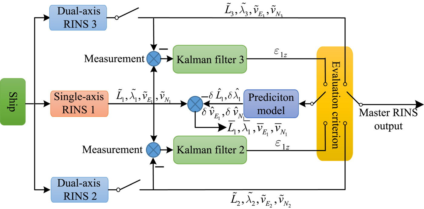
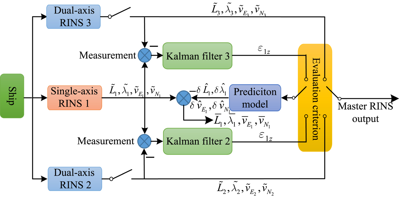
As shown in Figure 2, due to the higher reliability, the single-axis RINS 1 usually acts as a hot backup system for the dual-axis RINS 2. Based on the navigation information fusion between the two systems, the azimuth gyro drift of single-axis RINS 1 can be estimated and the position error caused by that can be predicted and compensated. In addition, all the inertial sensor biases estimated by the designed Kalman filter can be used to monitor the system running condition, and a built-in test procedure can diagnose the system faults. If the fault detection unit diagnoses a dual-axis RINS 2 failure, the position error caused by the single-axis RINS 1 constant azimuth gyro drift is still predicted, and the navigation information after compensation provided by the single-axis RINS 1 is adopted as the output.
Navigation information fusion in the dual RINS configuration.

The error state of the single-axis RINS 1 is represented as follows
 $${\bf x}_{1}(t)=[ \delta L_{1}, \delta \lambda_{1}, \delta v_{E_{1}}, \delta v_{N_{1}}, \phi_{E_1}, \phi_{N_1}, \phi_{U_1}]^T$$
The corresponding error state dynamic model is given by (Titterton and Weston, Reference Titterton and Weston2004)
 $$\dot{{\bf x}}_{1}(t) = {\bf A}_{1}(t){\bf x}_{1}(t) + {\bf B}_{1}(t){\bf u}_{1}(t) + {\bf G}_{1}(t){\bf w}_{1}(t)$$
with
 $${\bf A}_{1}(t) = \left[\matrix{{\bf F}_{1} & {\bf F}_{2} & 0_{2\times 3} \cr {\bf F}_{3} & {\bf F}_{4} & {\bf F}_{5} \cr {\bf F}_{7} & {\bf F}_{8} & {\bf F}_{9} }\right],\ {\bf B}_{1}(t)=\left[\matrix{0_{2\times 3} & 0_{2\times 2} \cr 0_{2\times 3} & \overline{{\bf C}}_{b_{1}}^{n} \cr -{\bf C}_{b_{1}}^{n} & 0_{3\times 2} }\right],\ {\bf G}_{1}(t)=\left[\matrix{0_{2\times 3} & 0_{2\times 2} \cr 0_{2\times 3} & \overline{{\bf C}}_{b_{1}}^{n} \cr -{\bf C}_{b_{1}}^{n} & 0_{3\times 2} }\right]$$
 $${\bf u}_{1}(t) = [\varepsilon_{1x},\varepsilon_{1y},\varepsilon_{1z},\ \nabla_{1x},\ \nabla_{1y}]^{T}\ {\bf w}_{1}(t)=[w_{\varepsilon_{1x}},w_{\varepsilon_{1y}},w_{\varepsilon_{1z}},w_{\nabla_{1x}},w_{\nabla_{1y}}]^{T}$$
where the sub-matrices of A1(t), B1(t) and G1(t) are the same forms as in the Appendix.
The gyro drifts and accelerometer biases of the single-axis RINS 1 can be estimated by the designed Kalman filter, whereby the deterministic position error can be predicted. Discretising Equation (30) (Simon, Reference Simon2006), the position error prediction model is given by
 $$\hat{\bf x}_{1} (k + 1) = {\bf \Phi}_{1}(k + 1, k) \hat{\bf x}_{1}(k) + {\bf \Gamma}_{1}(k) \hat{\bf u}_{1}(k)$$
with
 $$\eqalign{{\bf \Phi}_{1}(k + 1, k) &=e^{{\bf A}_{1} \delta t}, {\bf \Gamma}_{1}(k) = {\bf \Phi}_{1}(k + 1, k) \int_{0}^{\delta t}{\bi e}^{-{\bf A}_{1}\tau} d \tau {\bf B}_{1}, \cr \hat{{\bf u}}_{1}(k) &=[\hat{\varepsilon}_{1x}(k) \hat{\varepsilon}_{1y}(k) \hat{\varepsilon}_{1z}(k) \hat{\nabla}_{1x}(k) \hat{\nabla}_{1y}(k)]^{T}}$$
where  $\hat{\bf x}_{1}(k)$ is the error state prediction at time t k, and its initial value is set to
 $\hat{\bf x}_{1}(0) = 0; \hat{{\bf u}}_{1}(k)$ is the estimate of gyro drifts and accelerometer biases and Δ t is the discretisation step size. By subtracting the position error prediction from the position output of the single-axis RINS 1 as follows, its position accuracy can be improved to a certain extent:
 $$\overline{L_{1}} = \tilde{L}_{1}- \delta \hat{L}_{1}, \overline{\lambda_{1}} = \tilde{\lambda}_{1} - \delta \hat{\lambda}_{1}, \overline{v}_{E_{1}} = \tilde{v}_{E_{1}} - \delta \hat{v}_{E_{1}}, \overline{v}_{N_{1}} = \tilde{v}_{N_{1}} - \delta \hat{v}_{N_{1}}$$
The superscripts ‘-’ and ‘∧’ respectively denote correction value and prediction value.
4.2. Case II: the triple RINS configuration (single-axis RINS 1, dual-axis RINS 2 and 3)
In some special applications requiring particularly high reliability, a triple RINS configuration including two sets of dual-axis RINS and a single-axis RINS is needed. The only residual gyro error source is white-noise random drift, also known as angular random walk, which is the dominant factor determining the performance of a dual-axis RINS (Levinson and Majure, Reference Levinson and Majure1987). The angular random walk coefficients of the gyros used in the dual-axis RINS are usually close to each other, which makes the performance of different systems close to each other. As a result, the online performance of different systems during a voyage may not show consistency with previous test results. It is necessary to evaluate the performance of dual-axis RINS online to provide reference information for the ship operator.
As shown in Figure 3, two parallel computing Kalman filters are respectively built between the single-axis RINS 1 and the dual-axis RINS 2 as well as the dual-axis RINS 3 to estimate error states. The common error states of the two Kalman filters are the gyro drifts and accelerometer biases of the single-axis RINS 1.
Navigation information fusion in the triple RINS configuration.
The calculated state error covariance is given by the following Riccati equation (Gelb, Reference Gelb1974)
 $$\eqalign{\dot{{\bf P}}_{c}(t)&=[{\bf F}(t)-{\bf K}_{c}(t){\bf H}(t)]{\bf P}_{c}(t)+{\bf P}_{c}(t)[{\bf F}(t)-{\bf K}_{c}(t){\bf H}(t)]^{T} \cr &\quad +{\bf G}(t){\bf Q}_{c}{\bf G}^{T}(t)+{\bf K}_{c}(t){\bf RK}_{c}^{T}(t)}$$
where Kc(t) denotes the calculated gain, and Qc denotes the assumed process noise power spectral intensity. The process noise reflects the inertial sensors noise level including the dual-axis RINS gyro white-noise random drift. In practice, the correct process noise power spectral intensity is difficult to obtain, and the relationship between the assumed value and the actual value can be expressed as
 $${\bf Q}_{c} = (1 + \alpha) {\bf Q}$$
where α denotes a scalar (Simon, Reference Simon2006). Hence, the actual state error covariance is
 $$\eqalign{\dot{{\bf P}}_{a}(t) &=[{\bf F}(t)-{\bf K}_{c}(t){\bf H}(t)]{\bf P}_{a}(t)+{\bf P}_{a}(t)[{\bf F}(t)-{\bf K}_{c}(t){\bf H}(t)]^{T} \cr &\quad +{\bf G}(t){\bf Q}{\bf G}^{T}(t)+{\bf K}_{c}(t){\bf RK}_c^T}$$
where  ${\bf P}_{a}(t) = {\bf E}\{[{\bf x}_{a}(t)-\hat{{\bf x}}(t)][{\bf x}_{a}(t)-\hat{{\bf x}}(t)]^{T}\}$ denotes the actual state error covariance, and
 ${\bf x}_{a}(t)$ is the actual state. Subtracting Equation (38) from Equation (36) yields the differential equation of the difference between the actual and calculated covariance matrix as follows
 $$\Delta \dot{{\bf P}}(t)=\dot{{\bf P}}_{c}(t)-\dot{{\bf P}}_{a}(t)=[{\bf F}(t)-{\bf K}_{c}(t){\bf H}(t)] \Delta {\bf P}(t)+ \Delta {\bf P}(t)[{\bf F}(t)-{\bf K}_{c}(t){\bf H}(t)]^{T}+\alpha {\bf G}(t){\bf QG}^{T}(t)$$
An explicit analytic solution of Equation (39) is given by (Nishmura, Reference Nishmura1967)
 $$\Delta {\bf P}(t) = {\bf \phi}_{c}(t,0) \Delta {\bf P}(0){\bf \phi}_{c}^{T}(t,0) + \alpha \int_{0}^{t}{\bf \phi}_{c} (t,\tau){\bf G}(\tau){\bf QG}^{T}(\tau){\bf \Phi}_{c}^{T}(t,\tau){\bf d}\tau$$
where  $ \Delta {\bf P}(0)={\bf P}_{c}(0)-{\bf P}_{a}(0)={\bf 0},\ {\partial{\bf \Phi}_{c}(t,\tau) \over \partial t}=[{\bf F}(t) - {\bf K}_{c}(t){\bf H}(t)]{\bf \Phi}_{c}(t,\tau)$, and
 ${\bf \Phi}_{c}(t,t)={\bf I}$.
In practice,  ${\bf Q}_{c}\geq {\bf Q}$, that is, α≥0, usually applies to the tuning of the filter for conservative consideration. The second term in Equation (40) is semi-positive and
 ${\bf P}_{a}(t)={\bf P}_{c}(t)- \Delta {\bf P}(t)$, so the greater the actual process noise intensity, the smaller the scalar α, which results in a greater actual state error covariance, and the lower the actual process noise intensity, the greater the scalar α, which results in a smaller actual state error covariance.
Theoretically, the estimate of the gyro drifts and accelerometer biases of the single-axis RINS 1 in the two Kalman filters should be the same. However, as stated above, due to the uncertainty introduced by the process noise, their estimation accuracy may be different. Note that the only different process noise in the two Kalman filters is the dual-axis RINS gyro and accelerometer white-noise random drift. Instead of ensemble standard deviation, the time standard deviation of the common error state in the two Kalman filters can be used to evaluate the performance of the dual-axis RINS k(k=2, 3). In the case of stable gyro drift or slow-changing gyro drift, the smaller the time standard deviation, the lower the process noise intensity, which means the corresponding dual-axis RINS has better performance. However, if the gyro drift is very unstable, the smaller time deviation of the single-axis RINS does not necessarily mean the better performance of the dual-axis RINS. The time standard deviation of the single-axis RINS 1 azimuth gyro drift is selected as the criterion due to its higher estimation accuracy illustrated in Section 5.1.1. The corresponding calculation formula is given by
 $$\sigma_{k}(\hat{\varepsilon}_{1z}) = \sqrt{{1 \over N}\sum_{i=1}^{N}(\hat{\varepsilon}_{1z}-\mu_{\varepsilon_{1z}})^{2}}$$
where  $\sigma_{k} (\hat{\varepsilon}_{1z})(k = 2,3)$ denotes the standard deviation of the single-axis RINS 1 azimuth gyro drift estimate from the filter k, N is sampling number, and
 $\mu_{\varepsilon_{1z}}$ is the time average.
5. EXPERIMENTS RESULTS AND DISCUSSION
5.1. Case I: The Dual RINS Configuration (Single-axis RINS 1 and Dual-axis RINS 2)
5.1.1. Semi-physical experiment
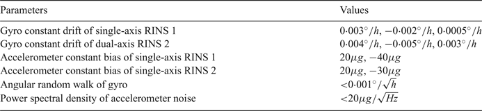
The initial conditions of the dual RINS configuration system are set as indicated in Table 1.
Parameters value.

The inertial sensor noise data is marine RINS static test data with the mean removed, which can reflect a real inertial sensor noise level. Both the single-axis RINS and the dual-axis RINS use the high-accuracy Ring Laser Gyro (RLG) as the attitude sensor. Due to the vertical channel's weak coupling with horizontal channels, only the horizontal accelerometer biases are taken into consideration.
The initial state error covariance matrix  ${\bf P}_{0}$ is set as:
 $${\bf P}_{0} = diag \left\{\matrix{(10m)^{2} (10m)^{2} (0{\cdot}05m/s)^{2} (0{\cdot}05m/s)^{2} (100^{\prime\prime})^{2} (100^{\prime\prime})^{2} (100^{\prime\prime})^{2}; \hfill \cr (0{\cdot}01^{\circ}/h)^{2} (0{\cdot}01^{\circ}/h)^{2} (0{\cdot}01^{\circ}/h)^{2} (0{\cdot}01^{\circ}/h)^{2} (0{\cdot}01^{\circ}/h)^{2} (0{\cdot}01^{\circ}/h)^{2}; \hfill \cr (50\mu g)^{2}\ (50\mu g)^{2}\ (50\mu g)^{2}\ (50\mu g)^{2} \hfill} \right\}$$
The measurement noise power spectral density is:
 $${\bf R} = diag \left\{(0{\cdot}2m/\sqrt{Hz})^{2} (0{\cdot}2m/\sqrt{Hz})^{2} (0{\cdot}02m/s/\sqrt{Hz})^{2} (0{\cdot}02m/s/\sqrt{Hz})^{2}\right\}$$
The process noise power spectral density is:
 $${\bf Q} = diag \left\{\matrix{(0{\cdot}001^{\circ}/\sqrt{h})^{2} (0{\cdot}001^{\circ}/\sqrt{h})^{2} (0{\cdot}001^{\circ}/\sqrt{h})^{2}; \hfill \cr (0{\cdot}001^{\circ}/\sqrt{h})^{2} (0{\cdot}001^{\circ}/\sqrt{h})^{2} (0{\cdot}001^{\circ}/\sqrt{h})^{2}; \hfill \cr (20\mu g/\sqrt{Hz})^{2} (20\mu g/\sqrt{Hz})^{2} (20\mu g/\sqrt{Hz})^{2} (20\mu g/\sqrt{Hz})^{2} \hfill} \right\}$$
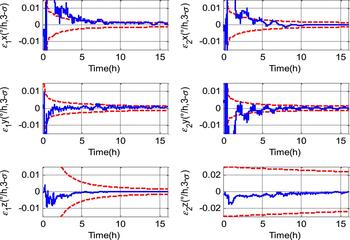
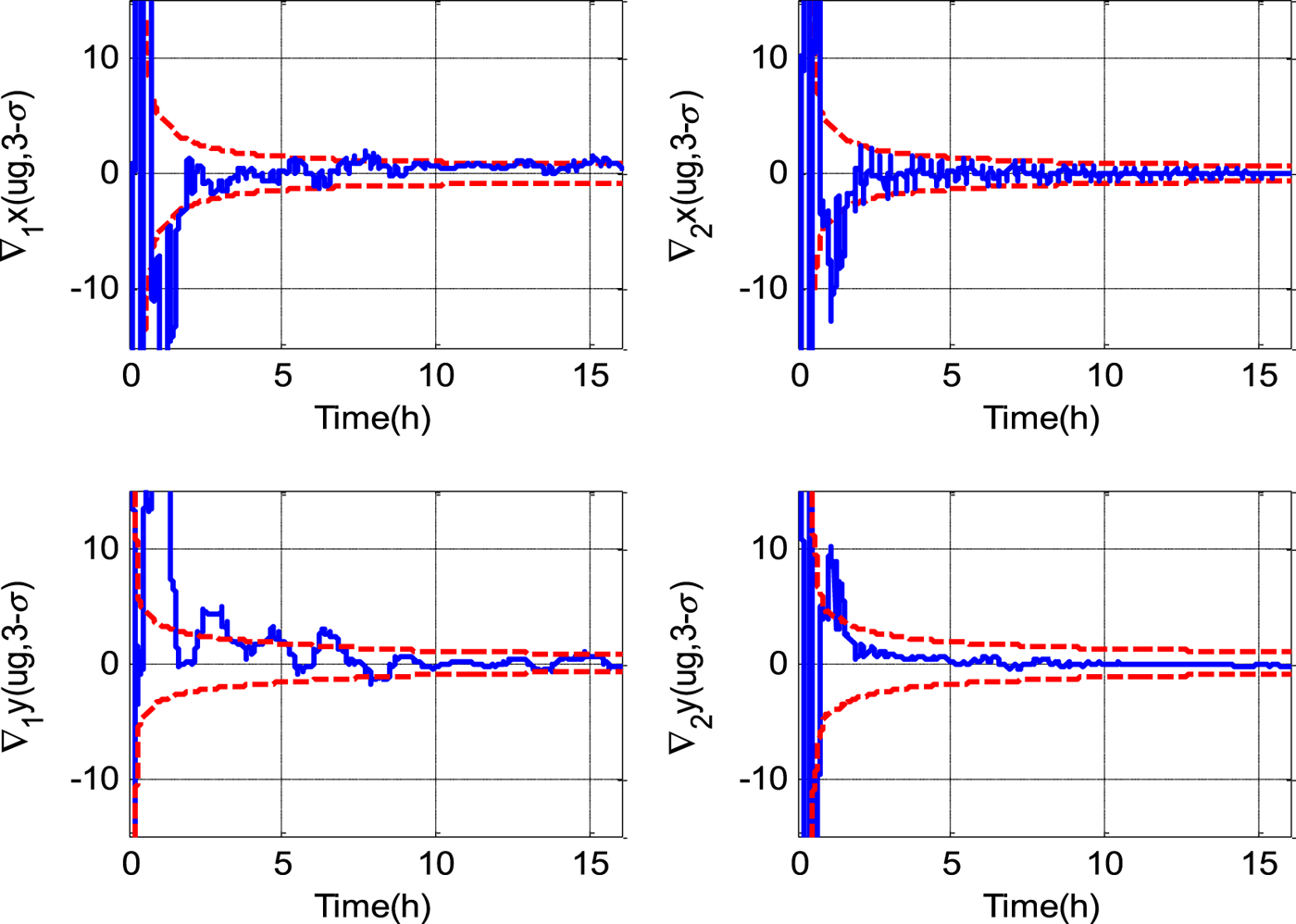
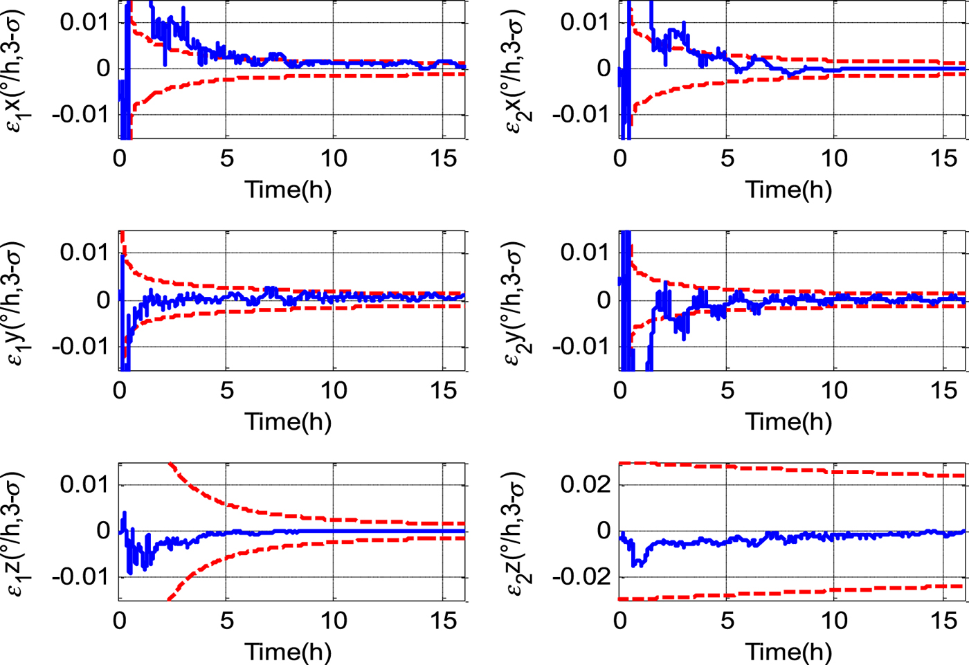
Supposing that the fault detection unit diagnoses the dual-axis RINS 2 failure at the sixteenth hour, the navigation information is provided by single-axis RINS 1 after that moment. Figure 4 depicts the gyro drift estimate errors of single-axis RINS 1 and dual-axis RINS 2 in the first 16 hours. The estimate errors for the horizontal gyro drifts of the single-axis RINS 1 and all the gyro drifts of dual-axis RINS 2 are less than 0·001°/h, while the estimate error for the azimuth gyro drift of single-axis RINS 1 is less than 0·00005°/h. The difference of estimate accuracy is due to the fact that all the gyro drifts are averaged out except the azimuth gyro drift of single-axis RINS 1, not distinctly influencing position error. In addition, the azimuth gyro drift of the single-axis RINS 1 takes about 12 hours (half of the Earth period) to reach 0·0001°/h accuracy, which is the same with the dockside alignment time of single-axis RINS in the general sense. As shown in Figure 5, the accelerometer bias estimate errors are less than 1 μ g. All the estimate errors are within their respective 3σ bounds.
Estimate errors for gyro drift and 3σ bounds.
Estimate errors for accelerometer bias and 3σ bounds.
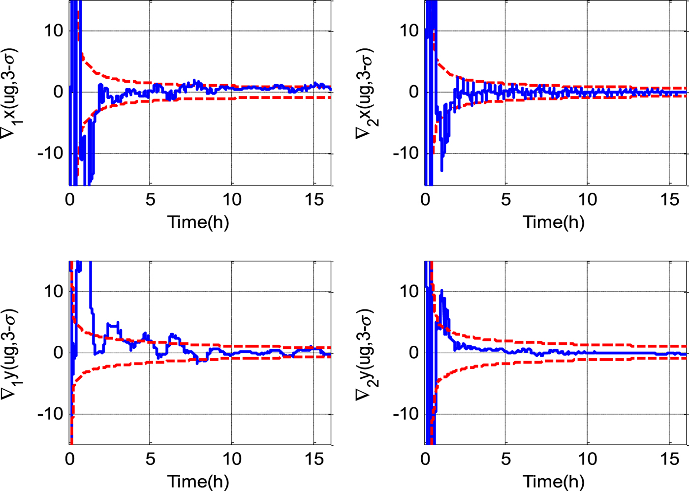
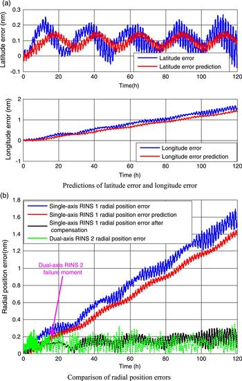
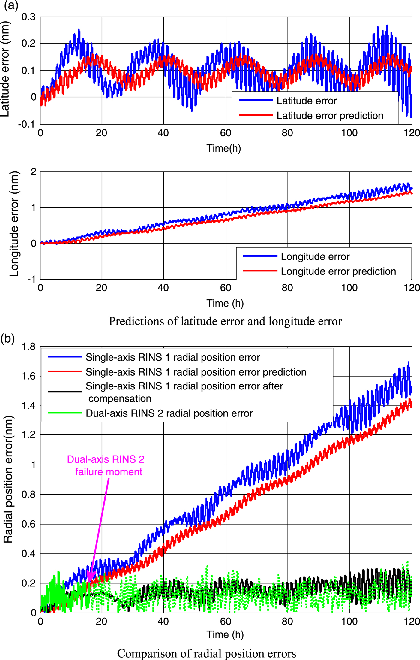
Figure 6(a) depicts the latitude error and longitude error of the single-axis RINS 1 as well as corresponding predictions. Figure 6(b) depicts the radial position errors of the single-axis RINS 1 and dual-axis RINS 2 over 120 hours. As shown, since the effect of the azimuth gyro drift cannot be averaged out in the single-axis RINS 1, it will lead to a position error proportional to the navigation time. However, after compensation for the deterministic position error prediction, the performance of the single-axis RINS 1 is greatly improved. Its position accuracy is comparable with the dual-axis RINS 2 whose radial position error will be illustrated by the green dotted line if no assumed failure happens to the dual-axis RINS 2. Hence, through navigation information fusion between the systems, the position accuracy can be guaranteed in the event of dual-axis RINS 2 failure.
Prediction of and compensation for the deterministic position error of single-axis RINS 1.
5.1.2. Laboratory test
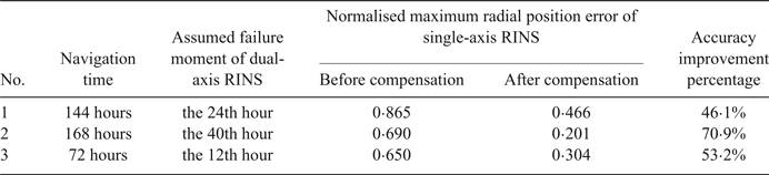
Three groups of static tests with different single-axis and dual-axis RINS were carried out to verify the proposed method in Section 4.1. Corresponding inertial sensor noise level is listed in Table 1. After alignment, all the systems work in the pure inertial navigation mode. As listed in Table 2, the navigation time of three groups of static tests is 144 hours (six days), 168 hours (seven days) and 72 hours (three days), respectively. The assumed failure moment of the dual-axis RINS is set at the twenty-fourth, the fortieth and the twelfth hour, respectively. This is followed by the fact that the navigation information is provided by the single-axis RINS which is the hot backup system after a failure. Table 2 also lists the normalised maximum radial position error before and after compensation for the position error prediction of the single-axis RINS, as well as the corresponding accuracy improvement percentage. As expected, the position accuracy of the single-axis RINS is greatly improved by compensating for the deterministic position error introduced by azimuth gyro drift.
Experimental descriptions and result statistics.
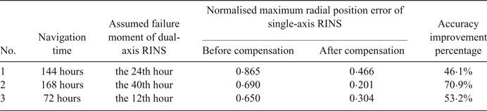
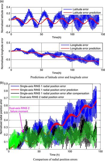
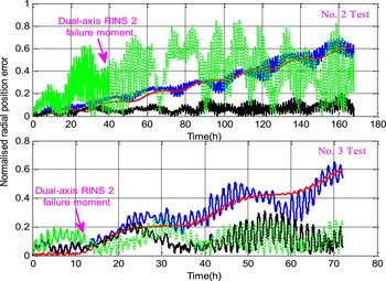
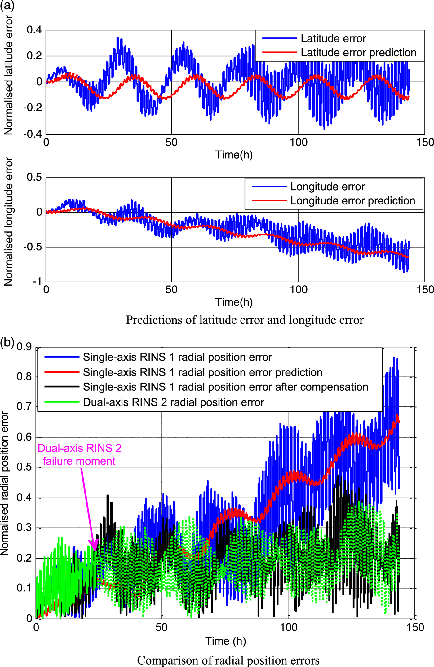
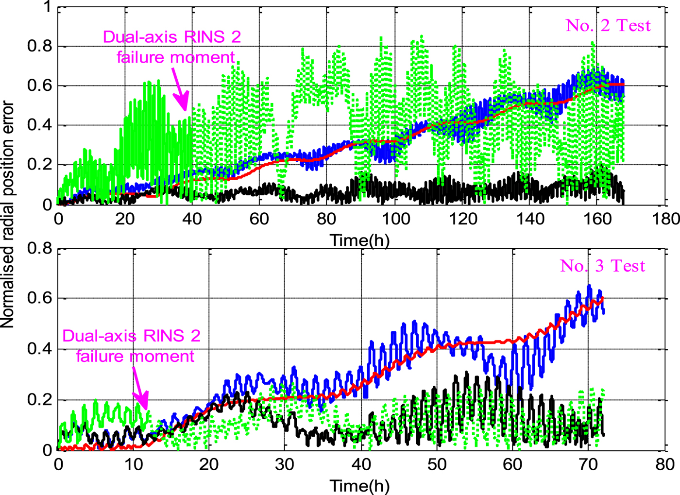
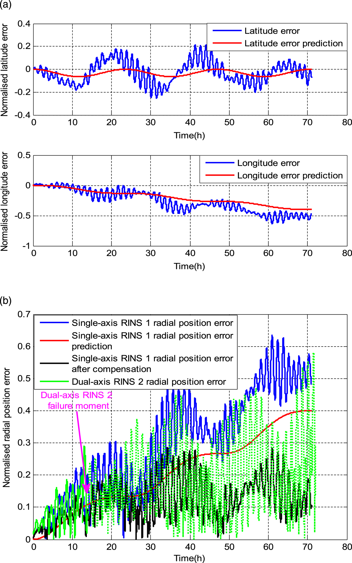
Figure 7(a) depicts the single-axis RINS’ latitude error, longitude error and their predictions in test 1. We can see that though there is some time lag in position error predictions (obvious in latitude error), the prediction model works well in the longitude error proportional to navigation time. Figure 7(b) depicts the radial position error of the single-axis RINS before and after compensation for the position error prediction in test 1. Similarly, Figure 8 shows the results in test 2 and test 3. As a comparison, the radial position error of the dual-axis RINS is depicted by the green dotted line if no assumed failure happens to the dual-axis RINS. It can be seen that the performance of the single-axis RINS after position error compensation is comparable with dual-axis RINS. Hence, with little or no accuracy loss, the improved performance single-axis RINS can guarantee position accuracy in the event of dual-axis RINS failure. Note that with the deterministic position error compensated, the performance of the single-axis RINS is better than the corresponding dual-axis RINS in test 2. The reason is that the gyro angular random walk of the single-axis RINS used in test 2 is less than that of the dual-axis RINS used in the same test, which makes the single-axis RINS’ statistic position error introduced by angular random walk less than that of the dual-axis RINS.
Prediction of and compensation for the deterministic position error of single-axis RINS 1 (Test 1).
Comparison radial position errors (Test 2 and Test 3).
5.1.3. At-sea test
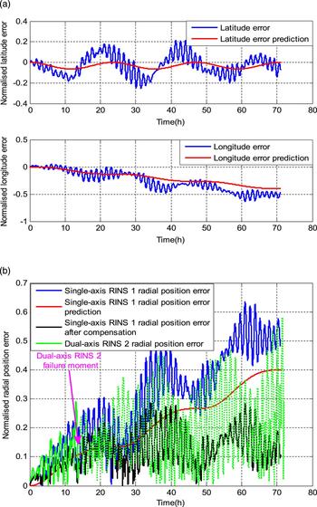
An at-sea test was conducted to verify the proposed method. After the alignment procedure, the single-axis RINS 1 and the dual-axis RINS 2 worked in the pure inertial navigation mode without any extemal benchmark information for correction. Test time was about 72 hours (three days). The Global Positioning System (GPS) information updated at 1 Hz is treated as the external position reference. The assumed failure moment of the dual-axis RINS 2 was the fourteenth hour, and the single-axis RINS 1 which is the hot backup system continued to provide position information for output after the assumed failure moment. As shown in Figure 9(a), the position error prediction model performs well, especially on the longitude error, which is caused by azimuth gyro drift and is proportional to navigation time. As shown in Figure 9(b), with the deterministic position error being compensated, the performance of single-axis RINS 1 was comparable or better than the dual-axis RINS 2. In this case, the performance of the single-axis RINS 1 mainly depends on its gyro angular random walk, as stated above. Hence, with little or no loss of accuracy, the position accuracy in the case of dual-axis RINS failure can be guaranteed by improving the performance of the single-axis RINS.
Prediction of and compensation for the deterministic position error of single-axis RINS 1 (At-sea test).
5.2. Case II: The Triple RINS Configuration (Single-axis RINS 1, Dual-axis RINS 2 and 3)
5.2.1. Sensitivity analysis
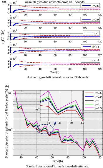
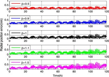
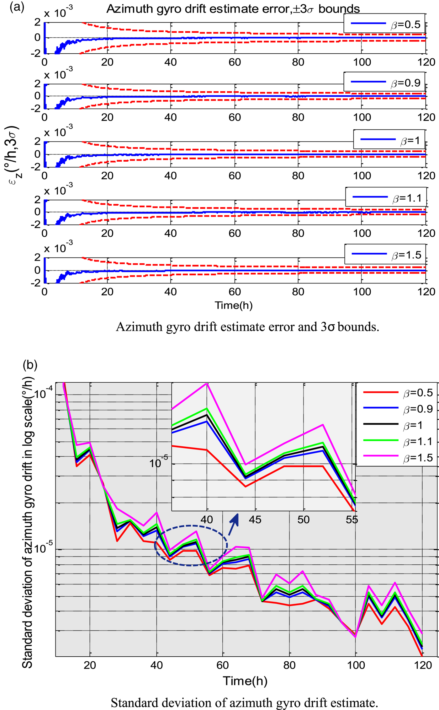
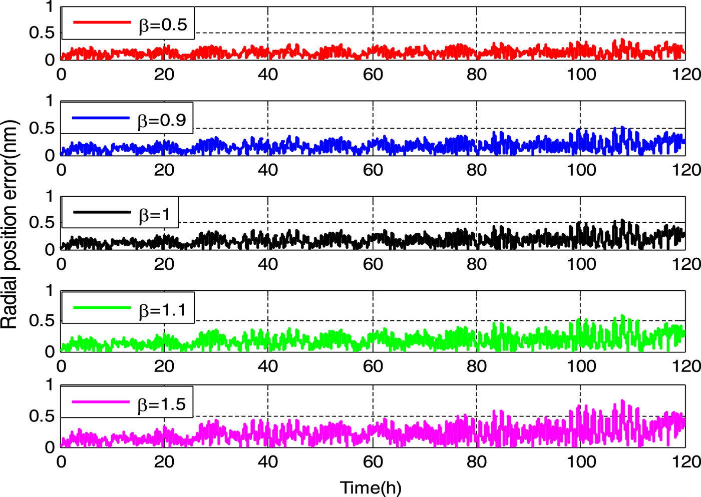
Semi-physical experiments were conducted to verify the online performance evaluation method for dual-axis RINS in the triple RINS configuration. The inertial sensor noise data was the marine RINS static test data with mean removed. As stated in Section 4.2, two parallel computing Kalman filters were built between the single-axis RINS and two sets of dual-axis RINS to estimate the azimuth gyro drift of the single-axis RINS. In order to evaluate the sensitivity of the aforementioned estimate standard deviation to the dual-axis RINS gyro noise intensity, the gyro noise data of dual-axis RINS were respectively multiplied by a coefficient β(β=0·5, 0·9, 1, 1·1, 1·5) to simulate different gyro noise intensity level. As shown in Figure 10(a), all the single-axis RINS azimuth gyro drift estimate errors were within 3σ bounds at different levels of dual-axis RINS gyro noise intensity. However, the online time standard deviation curves of azimuth gyro drift estimate present difference. Here, the standard deviation was calculated every four hours according to Equation (41). As expected, the greater the coefficient β, the greater the standard deviation of the azimuth gyro drift, which means the performance of dual-axis RINS was relatively bad. Figure 11 depicts the corresponding dual-axis RINS radial position error curves. Though we cannot distinguish the performances of dual-axis RINS at a glance, the online evaluation criterion gives a good measure, which can evaluate the performance of dual-axis RINS at different gyro noise levels even if there is only 10% difference of the gyro noise intensity.
Sensitivity of single-axis RINS azimuth gyro drift estimate to dual-axis RINS gyro noise intensity.
Radial position error of dual-axis RINS in different gyro noise intensity.
5.2.2. Experiment test
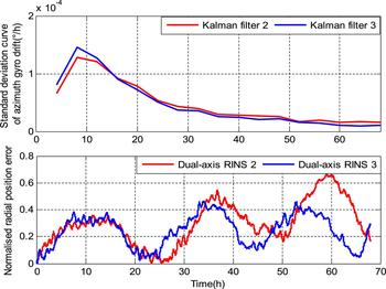
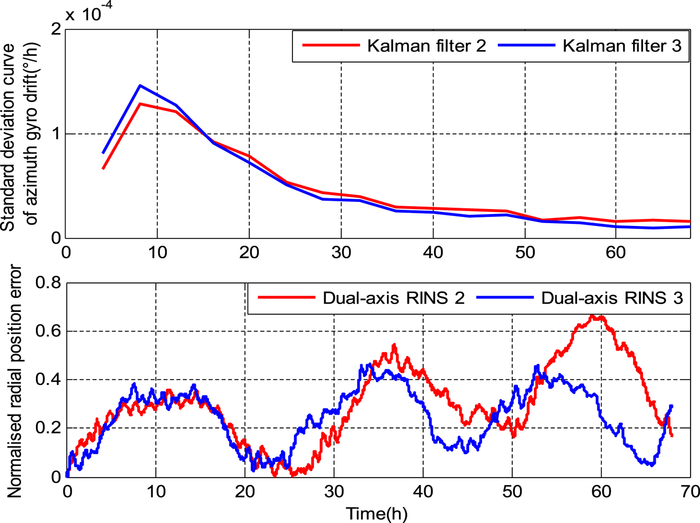
A laboratory test was conducted to verify the proposed method. We knew nothing about the performance of the dual-axis RINS in advance. Two Kalman filters, filter 2 and filter 3, are respectively built between the single-axis RINS 1 and the dual-axis RINS 2 as well as the dual-axis RINS 3 to estimate the azimuth gyro drift. Figure 12 shows the standard deviation curve of the single-axis RINS azimuth gyro drift estimate corresponding to Kalman filter 2 and 3. With the value calculated in filter 2 greater than that of filter 3, the performance of dual-axis RINS 3 should be better, which really shows consistency with the actual normalised radial position error depicted in Figure 12. The azimuth gyro drift estimate with the smaller standard deviation can be used to predict the position error of the single-axis RINS, and corresponding results are illustrated in Section 5.1, and is not repeated here.
Online performance evaluation of dual-axis RINS based on proposed criterion (static test).

5.2.3. At-sea test
An at-sea test was conducted to verify the proposed method. Test time was about 70 hours. The GPS information updated at 1 Hz was treated as the external position reference. As mentioned above, two Kalman filters are respectively constructed between the single-axis RINS 1 and the dual-axis RINS 2 as well as the dual-axis RINS 3 to estimate the azimuth gyro drift. Figure 13 depicts the standard deviation curve of the single-axis RINS azimuth gyro drift estimate corresponding to Kalman filter 2 and 3. The overall trend shows the value calculated in filter 2 was greater than that of filter 3, which means the performance of the dual-axis RINS 3 was better than that of the dual-axis RINS 2. As expected, the at-sea test result showed good consistency with laboratory test results. Namely, the better performance dual-axis RINS can be selected according to the consistency of single-axis RINS azimuth gyro drift estimate.
Online performance evaluation of dual-axis RINS based on proposed criterion (At-sea test).
6. CONCLUSIONS
In this paper, a novel navigation information fusion method based on an augmented error state Kalman filter was proposed for RINS redundant configuration. In dual RINS configuration, the position error prediction model of single-axis RINS was established to predict deterministic position error caused by azimuth gyro drift, whereby the position accuracy can be improved in the event of dual-axis RINS failure. In triple RINS configuration, two parallel computing augmented error state Kalman filters work to estimate the single-axis RINS azimuth gyro constant drift, and the consistency can be used as a criterion to select the better dual-axis RINS as the master RINS, which helps to avoid the ship operator's subjective choice. Similarly, the position accuracy of the single-axis RINS after error compensation is satisfactory even if both the dual-axis RINS fail simultaneously. Semi-physical experiments and tests showed that the navigation information fusion method works well.
Appendix
The system matrix of Equation (12) is given by
 $$\eqalign{{\bf F}(t) &= \left[\matrix{{\bf F}_{11}(t) &{\bf F}_{12}(t) \cr \hdashline \cr {\bf F}_{21}(t) &{\bf F}_{22}(t)} \right], {\bf F}_{11}(t) = \left[\matrix{{\bf F}_{1} & {\bf F}_{2} \cr {\bf F}_{3} & {\bf F}_{4} }\right], \cr {\bf F}_{12}(t)&=\left[\matrix{0_{2\times 3} & 0_{2\times 6} & 0_{2\times 4} \cr {\bf F}_{5} & 0_{2\times 6} & {\bf F}_{6} }\right], {\bf F}_{21}(t)=\left[\matrix{{\bf F}_{7} & {\bf F}_{8} \cr \hdashline \cr 0_{10\times 4}} \right]}$$
 $$\eqalign{{\bf F}_{22}(t) &= \left[\matrix{{\bf F}_{9} &{\bf F}_{10} &0_{3\times 4} \cr \hdashline \cr 0_{10\times 13}} \right], {\bf F}_1 = \left[\matrix{0 &0 \cr {v_E\tan L \over (R_E + h)\cos L} &0} \right], \cr {\bf F}_2 &= \left[\matrix{0 &{1 \over R_N+ h} \cr {1 \over (R_E + h)\cos L} &0} \right]}$$
 $$\eqalign{{\bf F}_{3} &= \left[\matrix{2\omega_{ie}v_{N}\cos L + {v_{N}v_{E} \over (R_{E}+h)\cos^{2}L} & 0 \cr -2\omega_{ie}v_{E}\cos L- {v_{E}^{2} \over (R_{E}+h)\cos^{2}L} & 0} \right], \cr {\bf F}_{4} &= \left[\matrix{{v_{N}\tan L \over R_{E} + h} &{v_{E}\tan L \over R_{E} + h} + 2\omega_{ie}\sin L \cr - 2\omega_{ie}\sin L - 2 {v_{E}\tan L \over R_{E}\,{+}\,h} &0} \right]}$$
 $$\eqalign{{\bf F}_{5}&=\left[\matrix{0 & -f_{U} & f_{N} \cr f_{U} & 0 & -f_{E} }\right],\ {\bf F}_{6}=[\overline{{\bf C}}_{b_{1}}^{n}\ -\overline{{\bf C}}_{b_{k}}^{n}],\ \matrix{\overline{{\bf C}}_{b_{1}}^{n}={\bf MC}_{b_{1}}^{n}{\bf M}^{{\rm T}} \cr \overline{{\bf C}}_{b_{k}}^{n}={\bf MC}_{b_{k}}^{n}{\bf M}^{{\rm T}} },{\bf M}=\left[ \matrix{1 & 0 & 0 \cr 0 & 1 & 0 }\right] \cr {\bf F}_{7}&=\left[\matrix{0 & 0 \cr -\omega_{ie}\sin L & 0 \cr \omega_{ie} \cos L+ {v_{E} \over (R_{E}+h)\cos^{2}L} & 0 }\right],\ {\bf F}_{8}=\left[ \matrix{0 &-{1 \over R_{E}+h} \cr {1 \over R_{E} + h} &0 \cr {\tan L \over R_{E}+h} &0}\right]}$$
 $$\eqalign{{\bf F}_{9}&=\left[ \matrix{0 &{v_{E}\tan L \over R_{E}+h}+\omega_{ie}\sin L &-\omega_{ie}\cos L- {v_{E} \over R_{E}+h} \cr - {v_{E}\tan L \over R_{E}+h}-\omega_{ie}\sin L &0 &-{v_{N} \over R_{N}+h} \cr \omega_{ie}\cos L+ {v_{E} \over R_{E}+h} &{v_{N} \over R_{N} + h} &0} \right], \cr {\bf F}_{10}&=[-{\bf C}_{b_{1}}^{n}\ {\bf C}_{b_{k}}^{n}]}$$
The process noise matrix is given by
 $${\bf G}(t) = \left[\matrix{0_{2\times 10} \cr \matrix{\hdashline \cr 0_{2\times 6} &\bar{{\bf C}}^n_{b_1} - \bar{\bf C}^n_{b_k} \cr \hdashline \cr -{\bf C}^n_{b_1} {\bf C}^n_{b_k} &0_{3\times 4} \cr \hdashline} \cr 0_{10\times 10}} \right]$$