1 Introduction
Modern gas turbine engines are characterised by their tight seal clearances to minimise purge flows. This characteristic has greatly increased the importance of understanding fluid flow and heat transfer phenomena in rotor–stator cavities. This interest includes both the under-platform cavities located under the rotor blades and stators and disk drum cavities. The cooling flow rate supplied to these cavities must be high enough to prevent them from being overheated, but small enough not to incur a large efficiency penalty in the engine thermodynamic cycle. There has been a great deal of design effort to minimise the cooling flow rate in order to achieve high thermal efficiency. Very sophisticated design systems have been developed in the past to deal with heat transfer problems in disks (Contreras, Corral & Pastor Reference Contreras, Corral and Pastor2011). These systems range from simple reduced-order models up to transient fully coupled computational fluid dynamics (CFD) and finite element (FE) conjugate analyses (Sun et al. Reference Sun, Chew, Hills, Volkov and Barnes2010, Reference Sun, Chew, Hills, Lewis and Mabilat2012; Ganine et al. Reference Ganine, Javiya, Hills and Chew2012). These complex analyses are intended to capture as closely as possible the physics of the problem, with the ultimate goal of improving the prediction capability of disk temperatures. Most of these analyses, with a few exceptions, assume that the fluid is quasi-stationary with respect to the solid. This hypothesis is used in both reduced-order models, which systematically make use of an experimental heat transfer coefficient, and CFD simulations, where the fluid temporal derivatives are neglected during the transient phase. This assumption is based on the hypothesis that the characteristic time of the fluid is much shorter than that of the solid, or the engine flight cycle. The motivation for this simplification is associated with the simulation cost, which has given rise to the analysis of optimal strategies to minimise the cost of the coupling (Corral & Wang Reference Corral and Wang2018). However, the physical basis of this strong hypothesis has not been properly assessed for transient cavity flows (Altuna et al. Reference Altuna, Chaquet, Corral, Gisbert and Pastor2013; Chaquet et al. Reference Chaquet, Corral, Gisbert and Pastor2015; Sun et al. Reference Sun, Amirante, Chew and Hills2016). The work reported here reviews the order of magnitude of the characteristic times involved in this process and presents numerical results for the first time of the thermal transient in a simplified rotor–stator cavity for engine representative non-dimensional parameters.
Losses due to windage have a direct impact on the performance of compressors and turbines and therefore in the overall efficiency of the engine. The term ‘windage’ is defined as the viscous friction drag and heating which result from the relative velocities across the boundary layers between the fluid and the rotating disk, and between the fluid and the stationary casing surfaces. The accurate quantification of heating due to windage in gas turbines is a well-recognised requirement for the successful design of modern engines, but the number of dedicated experiments is small (Tao et al. Reference Tao, Zhang, Luo, Xu and Han2014).
Rotating disk swirling flows are related to a number of fundamental issues in fluid dynamics. There have been many attempts to grasp this problem by deriving simplified models amenable to a theoretical treatment. By assuming the axial velocity to be radius-independent, von Kármán (Reference von Kármán1921) derived a set of ordinary differential equations (ODEs) describing the steady-state viscous flow above an infinite disk. Batchelor (Reference Batchelor1951) and Stewartson (Reference Stewartson1953) generalised von Kármán’s method to analyses concerned with flows between coaxial disks. The controversy about the existence of the two different solutions derived by Batchelor and Stewartson for infinite stator/rotor cavities has been thoroughly investigated (Mellor, Chapple & Stokes Reference Mellor, Chapple and Stokes1968; Zandbergen & Dijkstra Reference Zandbergen and Dijkstra1977; Holodniok, Kubi & Hlavá Reference Holodniok, Kubi and Hlavá1981; Kreiss & Parter Reference Kreiss and Parter1983). It was demonstrated numerically and analytically that both the Batchelor’s and Stewartson’s solutions could exist at high Reynolds numbers based on the gap in infinite cavities. The Bödewadt and von Kármán boundary layers are particular cases of stationary and rotating boundary-layer flows, respectively, that are exact solutions of the Navier–Stokes equations. These boundary-layer flows become unstable to two different instabilities, termed Type I and II, when
 $Re_{\unicode[STIX]{x1D6FF}}=U\unicode[STIX]{x1D6FF}/\unicode[STIX]{x1D708}$
exceeds a critical value, where
 $U$
is the reference velocity of the flow outside the boundary layer, and
 $\unicode[STIX]{x1D6FF}=(\unicode[STIX]{x1D708}/\unicode[STIX]{x1D6FA})^{1/2}$
the characteristic thickness of the boundary layer, where
 $\unicode[STIX]{x1D708}$
is the kinematic viscosity and
 $\unicode[STIX]{x1D714}$
is the angular velocity. Type I instability is related to an inflection point in the velocity profile, while Type II is viscous and associated with the Coriolis terms. In the case of infinite rotor–stator flow at large Reynolds number, based on the gap
 $s$
,
 $Re_{s}\sim (s/\unicode[STIX]{x1D6FF}_{c})^{2}\simeq 1000$
, the linear stability problem of the Batchelor flow is equivalent to the independent linear stability of both boundary layers separated by a rotating core at a swirl ratio of
 $\unicode[STIX]{x1D6FD}\simeq 0.31$
(Itoh et al.
Reference Itoh, Yamada, Imao and Gonda1992). Also, it was determined that the instability of Batchelor flow is initiated in the stationary Bödewadt boundary layer, at values of the critical Reynolds numbers,
 $Re_{\unicode[STIX]{x1D6FF}cI}\approx Re_{\unicode[STIX]{x1D6FF}cII}=35.5$
(Serre, Tuliszka-Sznitko & Bontoux Reference Serre, Tuliszka-Sznitko and Bontoux2004) for both Type I and II instabilities, much smaller than that which makes the rotating von Kármán boundary layer unstable. For separated boundary layers, this criterion translates into a critical Reynolds number based on the radius
 $Re_{\unicode[STIX]{x1D719}}=\unicode[STIX]{x1D6FA}r^{2}/\unicode[STIX]{x1D708}\sim 10^{5}$
. This actually means that laminar boundary layers can be seen in the innermost radii of gas turbine cavities.
With confined cavities, the outer shroud spoils the self-similar solution in the vicinity of the casing (Dijkstra & van Heijst Reference Dijkstra and van Heijst1983; Brady & Durlofsky Reference Brady and Durlofsky1987), although it is unclear that these perturbations affect the stability of the disk and stator boundary layers. A thorough review of the stability of rotor–stator cavities can be found in Launder, Poncet & Serre (Reference Launder, Poncet and Serre2010). The stability of Bödewadt’s boundary layer in confined cavities has been the subject of several studies (Lopez Reference Lopez1998; Lopez et al. Reference Lopez, Marques, Rubio and Avila2009), sometimes in conjunction with the spin-down process (Weidman Reference Weidman1976; Lopez & Weidman Reference Lopez and Weidman1996). Lopez et al. (Reference Lopez, Marques, Rubio and Avila2009) identified the instability mechanisms associated with the presence of spiral waves and axisymmetric circular waves, which are excited during the spin-down process, but that always die out at short times of the order of the diffusive time of the boundary layer.
The time-dependent problem of a single disk was analysed by Greenspan & Howard (Reference Greenspan and Howard1963), studying the process by which the state of rigid rotation of a viscous incompressible fluid in a closed, axially symmetric container was established. It was found that the transient phenomenon in this particular case consists of three distinct phases, namely, the development of the Ekman boundary layer for times
 $\unicode[STIX]{x1D70F}=\unicode[STIX]{x1D6FA}t\sim 1$
, the inviscid fluid spin-up
 $\unicode[STIX]{x1D70F}\sim (\unicode[STIX]{x1D6FA}L^{2}/\unicode[STIX]{x1D708})^{1/2}$
, and the viscous decay of residual effects in a dimensionless time
 $\unicode[STIX]{x1D70F}\sim (\unicode[STIX]{x1D6FA}L^{2}/\unicode[STIX]{x1D708})$
, where
 $L$
is a characteristic dimension, parallel to the axis of rotation. Fluid transients in disk cavities can be long, but this fact, although thoroughly researched in the past, has been overlooked recently. The literature related to true transients in rotor–stator cavities, despite their relevance, is nearly non-existent (Weidman Reference Weidman1976; van Eeten et al.
Reference van Eeten, van der Schaaf, van Heijst and Schouten2013). The work reported here reviews the order of magnitude of the characteristic times involved in this process, and presents numerical results for the first time in a simplified rotor–stator cavity for engine representative non-dimensional parameters. The objective is to elucidate whether or not the heat transfer behaviour of a disk transient can be computed using quasi-steady flow solutions and determine if this quasi-steady hypothesis holds.
The present work is structured as follows. Firstly, the system of ODEs governing the unsteady viscous flow between two large rotating disks when one of them is impulsively started is described. Secondly, the dedicated numerical method used to solve this set of ODEs is outlined. Thirdly, the method is used to obtain solutions at different Reynolds numbers and conclusions are drawn for the evolution of the velocity and temperature fields. Numerical simulations are supported with a theoretical analysis to ease the understanding of the underlying physics. Finally, two-dimensional laminar simulations for the transient velocity and temperature field in a rotor–stator cavity with a cylindrical housing are presented, and the results are compared with the self-similar solutions. It is confirmed that the two solutions compare well in the innermost region of the cavity and that the quasi-steady approximation of the fluid is only valid if the characteristic time of the transient
 $\unicode[STIX]{x1D6FA}t_{c}\gg (\unicode[STIX]{x1D6FA}s^{2}/\unicode[STIX]{x1D708})^{1/2}$
, which is a relevant conclusion for the computation of complex gas turbine cavity analyses.
2 One-dimensional analytical model
2.1 Governing equations
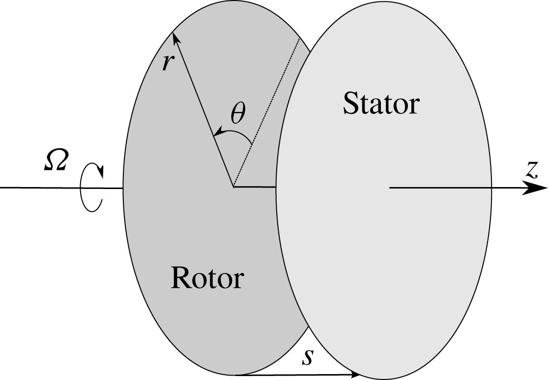
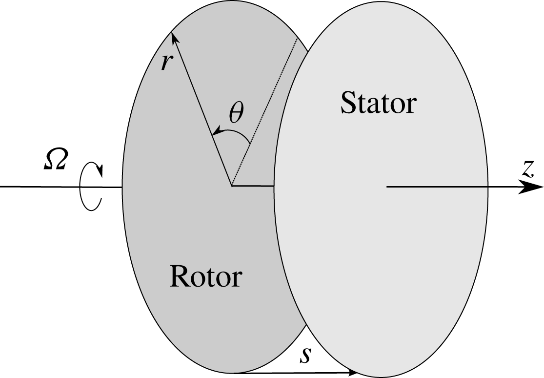
Let us consider two infinite coaxial disks separated by a spacing
 $s$
(see figure 1). A first disk, named rotor, rotates with angular velocity
 $\unicode[STIX]{x1D6FA}$
, whereas a second, named stator, is stationary. The wall temperatures of the rotor and the stator,
 $T_{R}$
and
 $T_{S}$
, respectively, are assumed to be uniform. The fluid has constant density,
 $\unicode[STIX]{x1D70C}$
, and kinematic viscosity,
 $\unicode[STIX]{x1D708}$
, and the flow is assumed to be laminar and axisymmetric.
Physical model of two coaxial rotating infinite disks.
2.1.1 Velocity field
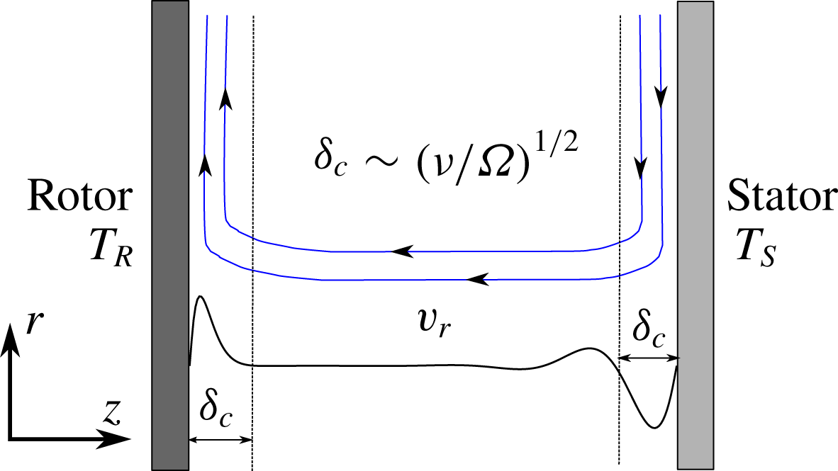
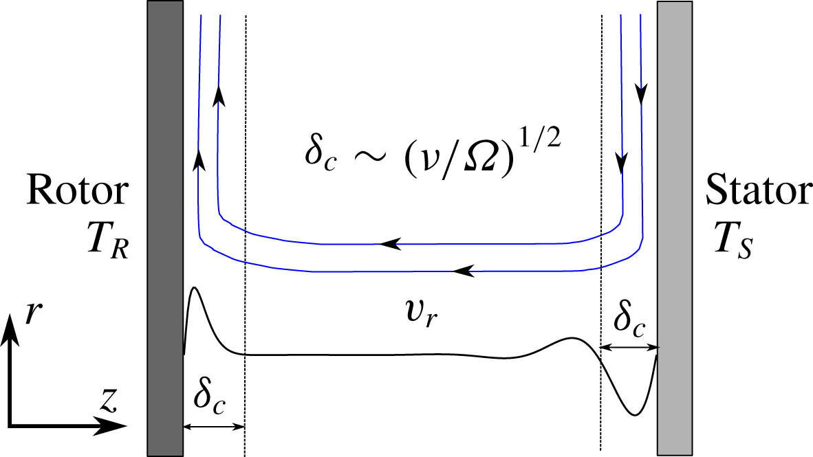
The flow pattern consists of two separated boundary layers attached to both disks if the Reynolds number is large enough (see figure 2). This allows simplification of the full Navier–Stokes equations using the boundary-layer approximation, where it is assumed that the flow variations in the radial direction are much smaller than in the wall-normal direction. This can be expressed in mathematical form as
 $\unicode[STIX]{x2202}_{r}\ll \unicode[STIX]{x2202}_{z}$
. The thin form of the continuity and momentum equations for incompressible and axisymmetric flow in cylindrical coordinates
 $(r,\unicode[STIX]{x1D703},z)$
, where
 $t$
is the physical time,
 $p$
is the pressure and
 $v$
is the velocity, is
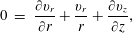 $$\begin{eqnarray}\displaystyle 0 & = & \displaystyle \frac{\unicode[STIX]{x2202}v_{r}}{\unicode[STIX]{x2202}r}+\frac{v_{r}}{r}+\frac{\unicode[STIX]{x2202}v_{z}}{\unicode[STIX]{x2202}z},\end{eqnarray}$$
 $$\begin{eqnarray}\displaystyle \frac{\unicode[STIX]{x2202}v_{r}}{\unicode[STIX]{x2202}t} & = & \displaystyle -v_{r}\frac{\unicode[STIX]{x2202}v_{r}}{\unicode[STIX]{x2202}r}-v_{z}\frac{\unicode[STIX]{x2202}v_{r}}{\unicode[STIX]{x2202}z}+\frac{v_{\unicode[STIX]{x1D703}}^{2}}{r}-\frac{1}{\unicode[STIX]{x1D70C}}\frac{\unicode[STIX]{x2202}p}{\unicode[STIX]{x2202}r}+\unicode[STIX]{x1D708}\left(\unicode[STIX]{x1D6FB}^{2}v_{r}-\frac{v_{r}}{r^{2}}\right),\end{eqnarray}$$
 $$\begin{eqnarray}\displaystyle \frac{\unicode[STIX]{x2202}v_{\unicode[STIX]{x1D703}}}{\unicode[STIX]{x2202}t} & = & \displaystyle -v_{r}\frac{\unicode[STIX]{x2202}v_{\unicode[STIX]{x1D703}}}{\unicode[STIX]{x2202}r}-v_{z}\frac{\unicode[STIX]{x2202}v_{\unicode[STIX]{x1D703}}}{\unicode[STIX]{x2202}z}-\frac{v_{r}v_{\unicode[STIX]{x1D703}}}{r}+\unicode[STIX]{x1D708}\left(\unicode[STIX]{x1D6FB}^{2}v_{\unicode[STIX]{x1D703}}-\frac{v_{\unicode[STIX]{x1D703}}}{r^{2}}\right),\end{eqnarray}$$
 $$\begin{eqnarray}\displaystyle \frac{\unicode[STIX]{x2202}v_{z}}{\unicode[STIX]{x2202}t} & = & \displaystyle -v_{r}\frac{\unicode[STIX]{x2202}v_{z}}{\unicode[STIX]{x2202}r}-v_{z}\frac{\unicode[STIX]{x2202}v_{z}}{\unicode[STIX]{x2202}z}-\frac{1}{\unicode[STIX]{x1D70C}}\frac{\unicode[STIX]{x2202}p}{\unicode[STIX]{x2202}z}+\unicode[STIX]{x1D708}\unicode[STIX]{x1D6FB}^{2}v_{z},\end{eqnarray}$$
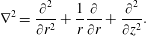 $$\begin{eqnarray}\unicode[STIX]{x1D6FB}^{2}=\frac{\unicode[STIX]{x2202}^{2}}{\unicode[STIX]{x2202}r^{2}}+\frac{1}{r}\frac{\unicode[STIX]{x2202}}{\unicode[STIX]{x2202}r}+\frac{\unicode[STIX]{x2202}^{2}}{\unicode[STIX]{x2202}z^{2}}.\end{eqnarray}$$
A similarity solution was found by von Kármán (Reference von Kármán1921) for an infinite rotating disk where the flow is at rest. By using this technique he managed to reduce the full Navier–Stokes equations to three nonlinear ordinary differential equations (ODEs). The similarity principle also applies if the fluid far away from the wall rotates as a rigid body (Batchelor Reference Batchelor1951) and even in the case of two infinite coaxial rotating disks, which is actually our case.
The velocity vector in a cylindrical system of coordinates in the absolute frame of reference can be written as
 $\boldsymbol{v}=v_{r}\boldsymbol{e}_{r}+v_{\unicode[STIX]{x1D703}}\boldsymbol{e}_{\unicode[STIX]{x1D703}}+v_{z}\boldsymbol{e}_{z}$
, where
 $\boldsymbol{e}_{r}$
,
 $\boldsymbol{e}_{\unicode[STIX]{x1D703}}$
and
 $\boldsymbol{e}_{z}$
, are unit vectors along the radial, circumferential and axial directions, respectively. In contrast to previous works (von Kármán Reference von Kármán1921; Batchelor Reference Batchelor1951), we allow variations of the velocity with time. According to well-established nomenclature, the three components of the velocity can be expressed as
 $$\begin{eqnarray}v_{r}=\unicode[STIX]{x1D6FA}rF(\unicode[STIX]{x1D709},\unicode[STIX]{x1D70F}),\quad v_{\unicode[STIX]{x1D703}}=\unicode[STIX]{x1D6FA}rG(\unicode[STIX]{x1D709},\unicode[STIX]{x1D70F}),\quad v_{z}=(\unicode[STIX]{x1D6FA}\unicode[STIX]{x1D708})^{1/2}H(\unicode[STIX]{x1D709},\unicode[STIX]{x1D70F}),\end{eqnarray}$$
where
 $F$
,
 $G$
and
 $H$
are, respectively, the dimensionless radial, circumferential and axial components of the velocity, and
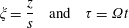 $$\begin{eqnarray}\unicode[STIX]{x1D709}=\frac{z}{s}\quad \text{and}\quad \unicode[STIX]{x1D70F}=\unicode[STIX]{x1D6FA}t\end{eqnarray}$$
are the dimensionless axial length and time. It is noteworthy that the characteristic velocity in the axial direction,
 $v_{zc}\sim (\unicode[STIX]{x1D6FA}\unicode[STIX]{x1D708})^{1/2}$
, is in general much smaller than the characteristic velocity in the radial and circumferential directions,
 $\unicode[STIX]{x1D6FA}r$
. The ratio between the two is
 $v_{\unicode[STIX]{x1D703}c}/v_{zc}\sim r_{c}/\unicode[STIX]{x1D6FF}_{c}$
, where
 $\unicode[STIX]{x1D6FF}_{c}\sim (\unicode[STIX]{x1D708}/\unicode[STIX]{x1D6FA})^{1/2}$
is the characteristic thickness of the disks’ boundary layers. The dimensionless pressure,
 $P(\unicode[STIX]{x1D709})$
, is defined as
 $$\begin{eqnarray}p=-\unicode[STIX]{x1D70C}(\unicode[STIX]{x1D708}\unicode[STIX]{x1D6FA})P(\unicode[STIX]{x1D709})+{\textstyle \frac{1}{2}}\unicode[STIX]{x1D70C}\unicode[STIX]{x1D714}_{core}^{2}r^{2},\end{eqnarray}$$
where
 $\unicode[STIX]{x1D714}_{core}$
is the angular velocity of the fluid in the core of the disk, which in general, for a rotor–stator cavity, is unknown. In the particular case of a rotating free disk
 $\unicode[STIX]{x1D714}_{core}=0$
. The static pressure is in the first approximation constant across the boundary layer, and it exhibits a quadratic function with the radius, since
 $\unicode[STIX]{x1D714}_{core}\sim \unicode[STIX]{x1D6FA}$
.
Sketch of the flow pattern between two infinite disks.
Substituting (2.3)–(2.5) into the thin form of the axisymmetric incompressible Navier–Stokes equations (2.1), we obtain
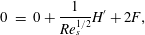 $$\begin{eqnarray}\displaystyle 0 & = & \displaystyle 0+\frac{1}{Re_{s}^{1/2}}H^{\prime }+2F,\end{eqnarray}$$
 $$\begin{eqnarray}\displaystyle \frac{\unicode[STIX]{x2202}F}{\unicode[STIX]{x2202}\unicode[STIX]{x1D70F}} & = & \displaystyle \frac{1}{Re_{s}}F^{\prime \prime }-\frac{1}{Re_{s}^{1/2}}F^{\prime }H+(G^{2}-F^{2})-\unicode[STIX]{x1D6FD}^{2},\end{eqnarray}$$
 $$\begin{eqnarray}\displaystyle \frac{\unicode[STIX]{x2202}G}{\unicode[STIX]{x2202}\unicode[STIX]{x1D70F}} & = & \displaystyle \frac{1}{Re_{s}}G^{\prime \prime }-\frac{1}{Re_{s}^{1/2}}G^{\prime }H-2FG,\end{eqnarray}$$
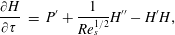 $$\begin{eqnarray}\displaystyle \frac{\unicode[STIX]{x2202}H}{\unicode[STIX]{x2202}\unicode[STIX]{x1D70F}} & = & \displaystyle P^{\prime }+\frac{1}{Re_{s}^{1/2}}H^{\prime \prime }-H^{\prime }H,\end{eqnarray}$$
 $Re_{s}$
is the Reynolds number based of the disk spacing
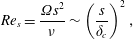 $$\begin{eqnarray}Re_{s}=\frac{\unicode[STIX]{x1D6FA}s^{2}}{\unicode[STIX]{x1D708}}\sim \left(\frac{s}{\unicode[STIX]{x1D6FF}_{c}}\right)^{2},\end{eqnarray}$$
which physically represents the square of the ratio between the disk spacing and the boundary-layer thickness. If
 $Re_{s}^{1/2}\gg 1$
, then the disk and stator boundary layers are confined to a thin region of the cavity of the order of
 $\unicode[STIX]{x1D6FF}_{c}/s\sim Re_{s}^{-1/2}$
. The swirl ratio,
 $\unicode[STIX]{x1D6FD}$
, appearing in the radial momentum equation, is defined as
 $$\begin{eqnarray}\unicode[STIX]{x1D6FD}=\unicode[STIX]{x1D714}_{core}/\unicode[STIX]{x1D6FA}.\end{eqnarray}$$
The origin of the swirl ratio
 $\unicode[STIX]{x1D6FD}$
, appearing in the radial momentum equation, and which is actually unknown, is due to the injection of expression (2.5) into the
 $\unicode[STIX]{x2202}p/\unicode[STIX]{x2202}r$
term of (2.1b
). Because the fluid is considered as incompressible and with constant properties, the continuity and momentum equations decouple from the energy equation and the flow pattern can be discussed independently of the temperature field. In the work presented here, buoyancy effects are disregarded, although they could be addressed following a similar formulation recurring to the Boussinesq approximation. This set of ODEs has to be integrated with the conditions that, at the rotating disk (
 $z=0$
)
 $\boldsymbol{v}=\unicode[STIX]{x1D6FA}r\boldsymbol{e}_{\unicode[STIX]{x1D703}}$
, and that at the stationary disk (
 $z=s$
)
 $\boldsymbol{v}=0$
. We also need to provide initial conditions for the problem compatible with the similarity hypothesis, hence at
 $t=0$
we will assume that
 $\boldsymbol{v}=\unicode[STIX]{x1D714}_{core}^{0}r\boldsymbol{e}_{r}$
, where
 $\unicode[STIX]{x1D714}_{core}^{0}$
is the angular velocity of the fluid at the initial instant. If we express these boundary and initial conditions in dimensionless form we obtain
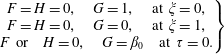 $$\begin{eqnarray}\left.\begin{array}{@{}c@{}}F=H=0,\quad G=1,\quad \text{at }\unicode[STIX]{x1D709}=0,\\ F=H=0,\quad G=0,\quad \text{at }\unicode[STIX]{x1D709}=1,\\ F\text{ or}\quad H=0,\quad G=\unicode[STIX]{x1D6FD}_{0}\quad \text{at }\unicode[STIX]{x1D70F}=0.\end{array}\right\}\end{eqnarray}$$
The problem reduces to one of finding the solution to (2.6a–c
), subject to the boundary conditions given in (2.9). It is important to recall at this point that, first, this system of equations needs just five boundary conditions, since the continuity equation does not contain any second derivative, but we have actually specified six. This extra boundary condition is used to determine the swirl factor
 $\unicode[STIX]{x1D6FD}$
, which is actually unknown. Secondly, only two initial conditions are needed as the continuity equation does not contain any time derivative and the dimensionless radial and axial velocities are strongly coupled through the mass conservation equation.
2.1.2 Energy equation
The energy equation of the axisymmetric form of the incompressible Navier–Stokes equations is
 $$\begin{eqnarray}\frac{\unicode[STIX]{x2202}T}{\unicode[STIX]{x2202}t}+v_{r}\frac{\unicode[STIX]{x2202}T}{\unicode[STIX]{x2202}r}+v_{z}\frac{\unicode[STIX]{x2202}T}{\unicode[STIX]{x2202}z}=\frac{k}{\unicode[STIX]{x1D70C}c}\unicode[STIX]{x1D6FB}^{2}T+\frac{\unicode[STIX]{x1D707}}{\unicode[STIX]{x1D70C}c}\unicode[STIX]{x1D6F7},\end{eqnarray}$$
where
 $c$
is the specific heat, and
 $\unicode[STIX]{x1D6F7}$
is Rayleigh’s dissipation function. If the thin form of the Navier–Stokes equations and expression (2.2) are used, then
 $\unicode[STIX]{x1D6FB}^{2}T\simeq \unicode[STIX]{x2202}^{2}T/\unicode[STIX]{x2202}z^{2}.$
The temperature field has to satisfy the following boundary conditions:
 $$\begin{eqnarray}T(\unicode[STIX]{x1D709}=0,\unicode[STIX]{x1D70F})=T_{R}\quad \text{and}\quad T(\unicode[STIX]{x1D709}=1,\unicode[STIX]{x1D70F})=T_{S}.\end{eqnarray}$$
We will also assume that at
 $\unicode[STIX]{x1D70F}=0$
,
 $T(\unicode[STIX]{x1D709})=T_{s}$
. The temperature can be decomposed as
 $$\begin{eqnarray}T(\unicode[STIX]{x1D709},r,\unicode[STIX]{x1D70F})=T_{0}(\unicode[STIX]{x1D709},\unicode[STIX]{x1D70F})+\left(\frac{r}{s}\right)^{2}T_{2}(\unicode[STIX]{x1D709},\unicode[STIX]{x1D70F}),\end{eqnarray}$$
where the quadratic radial variation of the temperature is explicitly retained. The dimensionless temperature,
 $\tilde{T}$
, can be written as
 $$\begin{eqnarray}\tilde{T}=\frac{T-T_{S}}{T_{R}-T_{S}}=\frac{T_{0}-T_{S}}{T_{R}-T_{s}}+\left(\frac{r}{s}\right)^{2}\frac{T_{2}}{T_{R}-T_{s}}=\tilde{T}_{0}+\tilde{r}^{2}\tilde{T}_{2}.\end{eqnarray}$$
Injecting the previous expression in the energy equation and identifying terms in
 $\tilde{r}^{0}$
and
 $\tilde{r}^{2}$
, we obtain the following evolution equation for
 $\tilde{T}_{0}$
:
 $$\begin{eqnarray}\frac{\unicode[STIX]{x2202}\tilde{T}_{0}}{\unicode[STIX]{x2202}\unicode[STIX]{x1D70F}}+\frac{1}{Re_{s}^{1/2}}H\widetilde{T}_{0}^{\prime }=\frac{1}{Pr\,Re_{s}}(\tilde{T}_{0}^{\prime \prime }+4\tilde{T}_{2})+\frac{Ec}{Re_{s}}12F^{2}.\end{eqnarray}$$
This has to be solved with the boundary conditions
 $\tilde{T_{0}}=1$
at
 $\unicode[STIX]{x1D709}=0$
and
 $\tilde{T_{0}}=0$
at
 $\unicode[STIX]{x1D709}=1$
. The equivalent equation for
 $\tilde{T}_{2}$
reads
 $$\begin{eqnarray}\frac{\unicode[STIX]{x2202}\tilde{T}_{2}}{\unicode[STIX]{x2202}\unicode[STIX]{x1D70F}}+\frac{1}{Re_{s}^{1/2}}H\widetilde{T}_{2}^{\prime }+2F\tilde{T_{2}}=\frac{1}{Pr\,Re_{s}}\tilde{T}_{2}^{\prime \prime }+\frac{Ec}{Re_{s}}(G^{\prime 2}+F^{\prime 2}),\end{eqnarray}$$
with the boundary conditions
 $\tilde{T_{2}}=0$
at
 $\unicode[STIX]{x1D709}=0$
and
 $\tilde{T_{2}}=0$
at
 $\unicode[STIX]{x1D709}=1$
. The order of magnitude of the ratio of the viscous dissipation and the heat conduction is
 $Pr\,Ec$
, where the Eckert parameter, is defined as
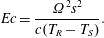 $$\begin{eqnarray}Ec=\frac{\unicode[STIX]{x1D6FA}^{2}s^{2}}{c(T_{R}-T_{S})}.\end{eqnarray}$$
If the Eckert number is zero, or small, viscous dissipation is much smaller than the conduction and can be neglected. The solution of (2.15) is in this case
 $\tilde{T}_{2}=0$
, physically meaning that the heating due to the windage is negligible. It can be shown that
 $\tilde{T}_{2}\sim Pr\,E_{c}\backsimeq E_{c}$
, if
 $Pr\sim \mathit{O}(1)$
, as is actually the case for air and other gases. In this case
 $\tilde{T}_{2}/\tilde{T}_{0}^{\prime \prime }$
 ${\sim}Ec/Re_{s}\ll 1$
, and then (2.14) decouples from (2.15), and can be solved independently. However, the true relative weight of
 $\tilde{T}_{0}$
and
 $\tilde{T}_{2}$
depends on the dimensionless radius,
 $\tilde{r},$
which can actually be large, and hence, even if
 $\tilde{T}_{2}\ll \tilde{T}_{0}$
,
 $\tilde{T}_{0}\sim \tilde{r}^{2}\tilde{T}_{2}$
. It is important to note as well that if
 $Ec/Re_{s}\ll 1$
, viscous dissipation can be neglected as well in the equation for
 $\tilde{T}_{0}$
, equation (2.14). The energy equation is then linear and effects can be superimposed. The equation for
 $\tilde{T}_{0}$
can be decomposed into the solution of an homogeneous part,
 $\unicode[STIX]{x1D6FC}$
, and a particular solution,
 $K$
. The temperature field is then given by
 $$\begin{eqnarray}\tilde{T}(\unicode[STIX]{x1D709})=\unicode[STIX]{x1D6FC}(\unicode[STIX]{x1D709})+Ec\,K(\unicode[STIX]{x1D709})+\tilde{r}^{2}Ec\,\hat{T}_{2}(\unicode[STIX]{x1D709})\end{eqnarray}$$
and the heat flux by
 $$\begin{eqnarray}q=k\frac{(T_{R}-T_{S})}{s}(\unicode[STIX]{x1D6FC}_{w}^{\prime |}+Ec\,K^{\prime }+\tilde{r}^{2}\,Ec\,\hat{T}_{2w}^{\prime })\end{eqnarray}$$
with
 $\hat{T}_{2}=\tilde{T}_{2}/Ec$
. It is readily seen that only the first term of (2.18) is proportional to
 $\unicode[STIX]{x0394}T$
, and that
 $\hat{T}_{2}$
is not controlled by any temperature difference, but by viscous heating.
2.1.3 Numerical method
The set of nonlinear time-dependent ODEs defined by (2.6), (2.14) and (2.15) is discretised using a second-order method, both in space and time. Firstly, the radial momentum equation (2.6b
) is derived with respect
 $\unicode[STIX]{x1D709}$
to eliminate its explicit dependence on the swirl factor,
 $\unicode[STIX]{x1D6FD}$
,
 $$\begin{eqnarray}\frac{\unicode[STIX]{x2202}F^{\prime }}{\unicode[STIX]{x2202}\unicode[STIX]{x1D70F}}=\frac{1}{Re_{s}}F^{\prime \prime \prime }-\frac{1}{Re_{s}^{1/2}}F^{\prime \prime }H-\frac{1}{Re_{s}^{1/2}}F^{\prime }H^{\prime }+2GG^{\prime }-2FF^{\prime },\end{eqnarray}$$
and, secondly, the continuity equation (2.6a
),
 $F=-2Re_{s}^{1/2}H^{\prime }$
, is used to eliminate the dimensionless radial velocity,
 $F$
, from the formulation. As a result, the following expression for the derivative of the radial momentum equation is obtained:
 $$\begin{eqnarray}\frac{1}{Re_{s}}H^{(iv)}-\frac{\unicode[STIX]{x2202}H^{\prime \prime }}{\unicode[STIX]{x2202}\unicode[STIX]{x1D70F}}=4Re_{s}^{1/2}GG^{\prime }+\frac{1}{Re_{s}^{1/2}}HH^{\prime \prime \prime }=R_{H}(H,G),\end{eqnarray}$$
which has to be solved with the condition that
 $H=H^{\prime }=0$
at
 $\unicode[STIX]{x1D709}=0$
and
 $\unicode[STIX]{x1D709}=1$
, The time derivative is discretised using second-order backwards differentiation:
 $$\begin{eqnarray}\left(\frac{\unicode[STIX]{x2202}H^{\prime \prime }}{\unicode[STIX]{x2202}\unicode[STIX]{x1D70F}}\right)^{n+1}=\frac{3(H^{\prime \prime })^{n+1}-4(H^{\prime \prime })^{n}+(H^{\prime \prime })^{n-1}}{2\unicode[STIX]{x0394}\unicode[STIX]{x1D70F}}.\end{eqnarray}$$
A fully implicit method is constructed expressing the left-hand side of (2.20) at instant
 $n+1$
to obtain
 $$\begin{eqnarray}\frac{1}{Re_{s}}(H^{(iv)})^{n+1}-\left(\frac{\unicode[STIX]{x2202}H^{\prime \prime }}{\unicode[STIX]{x2202}\unicode[STIX]{x1D70F}}\right)^{n+1}=R_{H}^{n+1}.\end{eqnarray}$$
Spatial derivatives are discretised using second-order central finite differences. The resulting system of nonlinear algebraic equations is solved using a fixed point iteration method. The nonlinear right-hand side of (2.22) is evaluated in the previous step of the fixed point iteration process,
 $m$
, leading to
 $$\begin{eqnarray}\frac{1}{Re_{s}}(H^{(iv)})_{m+1}^{n+1}-\left(\frac{\unicode[STIX]{x2202}H^{\prime \prime }}{\unicode[STIX]{x2202}\unicode[STIX]{x1D70F}}\right)_{m+1}^{n+1}=R_{H}^{n+1}(G_{m},H_{m}),\end{eqnarray}$$
which requires the solution of a pentadiagonal system of linear equations, per iteration. The system is converged to machine accuracy before advancing to the next time step.
The circumferential momentum equation is solved analogously:
 $$\begin{eqnarray}\frac{1}{Re_{s}}(G^{\prime \prime })_{m+1}^{n+1}-\left(\frac{\unicode[STIX]{x2202}G}{\unicode[STIX]{x2202}\unicode[STIX]{x1D70F}}\right)_{m+1}^{n+1}=R_{G}^{n+1}(G_{m},H_{m}).\end{eqnarray}$$
It has to be solved with the condition that
 $G=1$
at
 $\unicode[STIX]{x1D709}=0$
, and
 $G=0$
at
 $\unicode[STIX]{x1D709}=1$
. In this case (2.24) represents a tridiagonal system of linear equations. Equations (2.23) and (2.24) are solved simultaneously. Once the velocity field is obtained, the energy equations (2.14) and (2.15) are solved using a similar approach, although in this case the fixed point iteration method is not needed since the energy equation is linear.
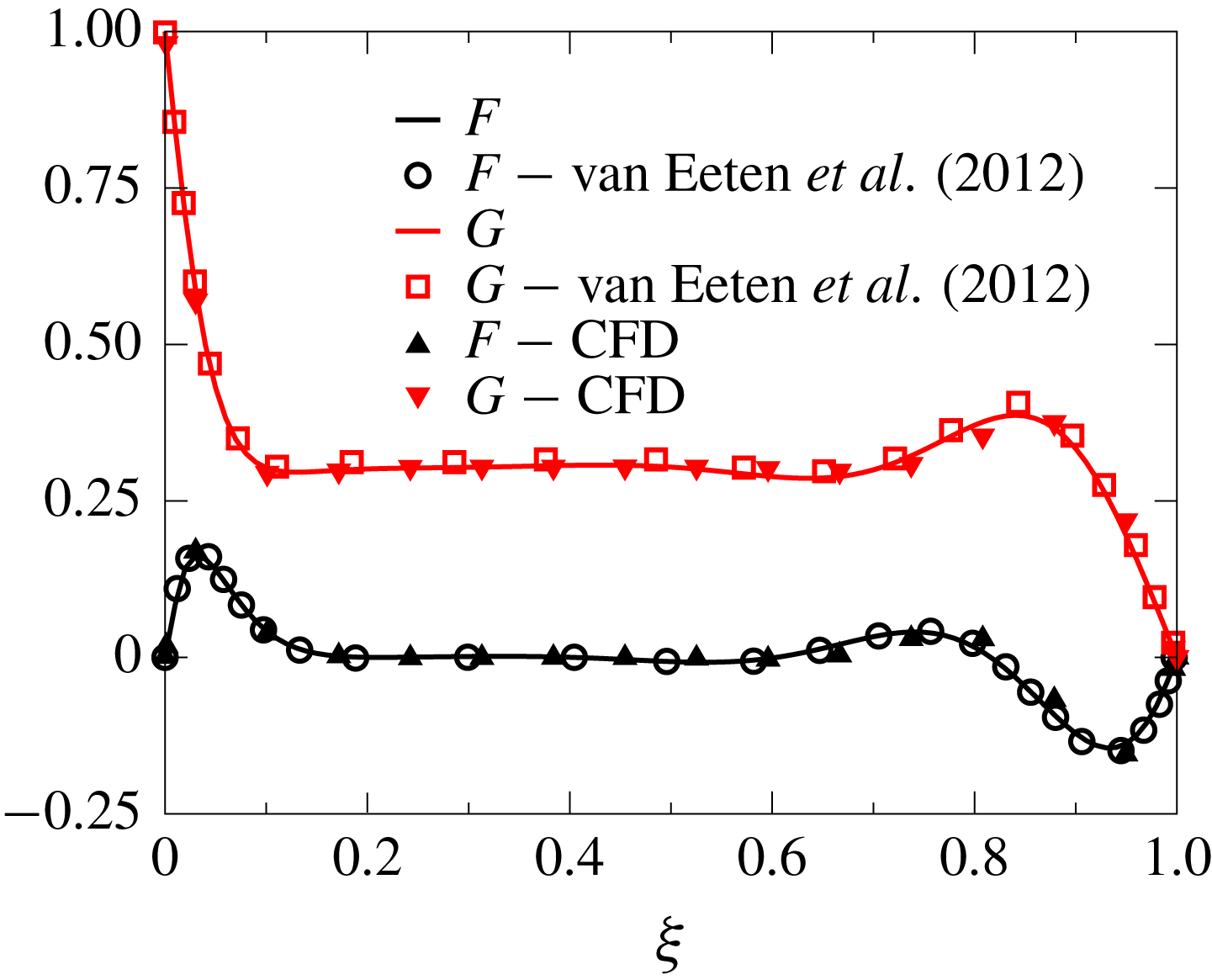
Dimensionless radial (
 $F$
) and circumferential (
 $G$
) velocity distributions for a rotor–stator cavity rotating at
 $Re_{s}=975$
.
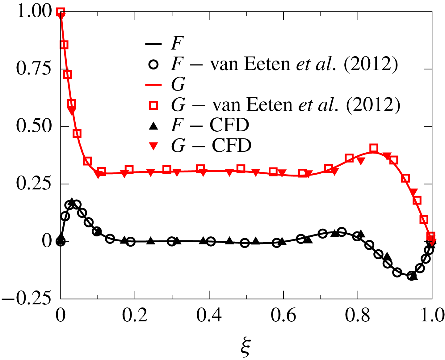
Numerical accuracy has been checked against well-known solutions for a free rotating disk with different swirl factors at infinity. Figure 3 compares the dimensionless velocity distributions computed with the present method for two infinite disks, one rotating and the other stationary, at
 $Re_{s}=975$
, with the solutions obtained by van Eeten et al. (Reference van Eeten, van der Schaaf, Schouten and van Heijst2012) and CFD results. It can be seen that the agreement between all of the cases is very good.
2.2 Results
The purpose of this section is to numerically and theoretically investigate the transient behaviour of a model laminar rotor–stator cavity at high Reynolds numbers using a similarity solution. Although it is well known that this type of flow rapidly experiences instabilities and transition to turbulence, still there is value in understanding different trends with the Reynolds number as a previous conceptual step to dealing with the more involved and realistic problem of turbulent cavities. From a conceptual point of view, if
 $Re_{s}$
is large enough but smaller than the critical transition Reynolds number, the scaling laws for a laminar flow do not change. In the limit of high rotation rate, the flow between a stationary and a rotating disk presents two separated boundary layers, the so-called Bödewadt and von Kármán boundary layers respectively, which can transition to the turbulent regime at moderate local Reynolds number
 $Re_{\unicode[STIX]{x1D719}}^{c}$
. An important remark is that the effect of the local Reynolds number in the flow is independent of
 $Re_{s}$
, as long as this is large enough to obtain separated boundary layers (
 $Re_{s}\gtrapprox 500$
); see Launder et al. (Reference Launder, Poncet and Serre2010). If
 $Re_{\unicode[STIX]{x1D719}}>Re_{\unicode[STIX]{x1D719}}^{c}$
the flow becomes turbulent and the scaling laws with
 $Re_{s}$
change, but this point is not covered in the analytical work. For this reason, we have decided to conduct most of the analyses at high, but modest, Reynolds numbers based on the gap, to capture the asymptotic trends with
 $Re_{s}$
, but remaining within the laminar regime. The extrapolation to higher
 $Re_{s}$
, but remaining in the laminar regime, is trivial.
2.2.1 Stationary solutions
Numerical results have been obtained for Reynolds gap numbers ranging between 600 and 30 000 to verify different trends with
 $Re_{s}$
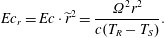
. The product of the Eckert number and the dimensionless radial distance based on the gap,
 $E_{c}\cdot \tilde{r}^{2}$
, appearing in (2.17) is the Eckert number based on the radius:
 $$\begin{eqnarray}Ec_{r}=Ec\cdot \widetilde{r}^{2}=\frac{\unicode[STIX]{x1D6FA}^{2}r^{2}}{c(T_{R}-T_{S})}.\end{eqnarray}$$
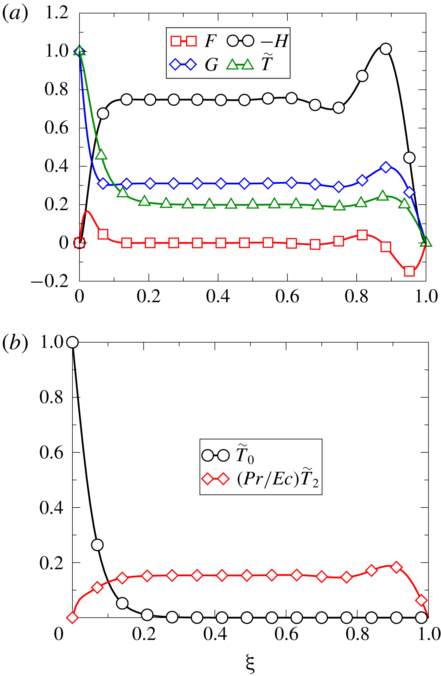
Figure 4 shows the numerical solution of the Batchelor’s flow for
 $Re_{s}=2000$
,
 $Pr=0.71$
and
 $Ec_{r}=1$
. For gas turbine applications, whose working fluid is air, the Prandtl number is fairly constant in a large temperature range, and therefore its variation lacks interest and has not been pursued in this work.
Dimensionless velocity components (a) and temperature field components
 $\tilde{T}_{0}$
and
 $\tilde{T}_{2}$
(b) at
 $Re_{s}=2000$
,
 $Pr=0.71$
,
 $Ec_{r}=1$
and
 $\tilde{r}=5$
.
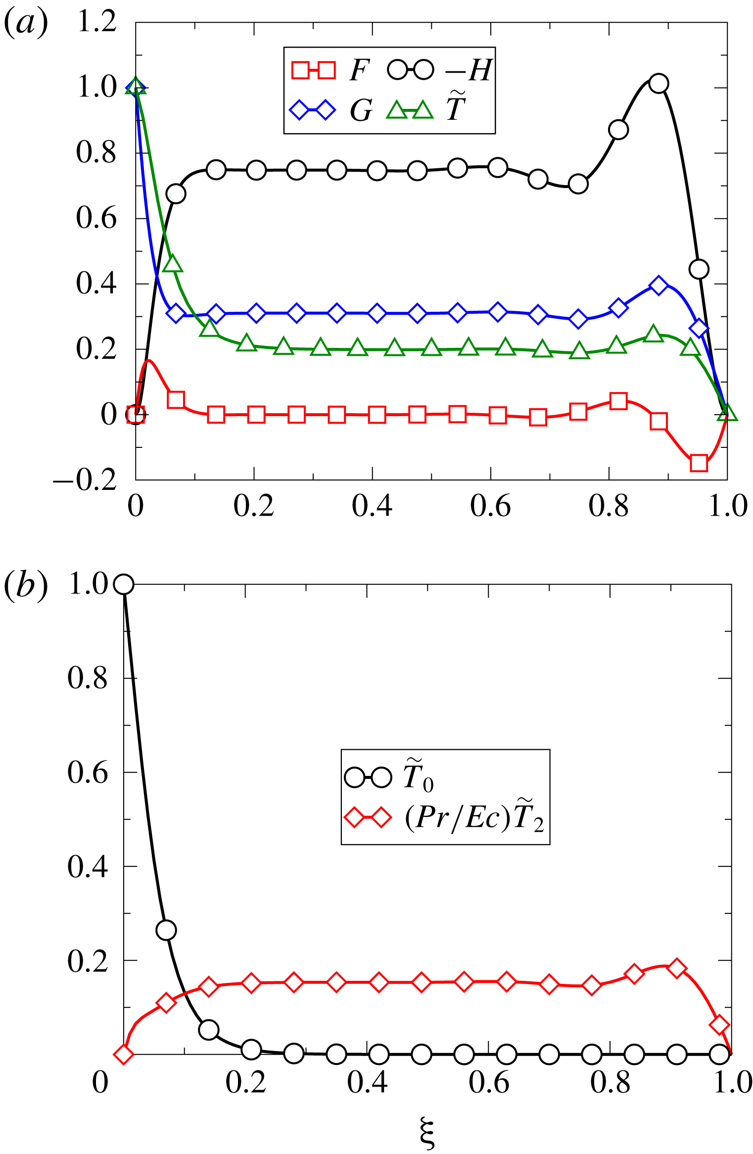
Figure 2 sketches the flow pattern within two infinite disks. Fluid is pumped outwards by the rotor motion through a thin layer, sometimes referred to in the literature as von Kármán’s boundary layer. This thin region is fed by a central part, where viscous effects are negligible, which is termed here the core region. The fluid in this core region, to a first approximation, rotates as a rigid body with constant angular velocity and null radial velocity. There is a second thin region in the stator, generally termed Bödewadt’s boundary layer (Bödewadt Reference Bödewadt1940), with fluid moving inwards, to exactly compensate for the fluid expelled out by the rotor, finally enforcing the no-slip boundary condition at the wall. The relative thickness of these boundary layers with respect to the disk spacing is obtained by balancing the convective and viscous terms in the momentum equation,
 $\unicode[STIX]{x1D6FF}_{c}/s\sim Re_{s}^{-1/2}.$
Figure 4(a) also displays the temperature profile for the same case, where the three regions previously described for the velocity distribution can be noticed. The thermal boundary-layer thickness,
 $\unicode[STIX]{x1D6FF}_{T}$
, is of order
 $\unicode[STIX]{x1D6FF}_{T}/s\sim (Re_{s}Pr)^{-1/2}$
, in our case, since
 $Pr\simeq 1$
, both boundary-layer thicknesses are of the same order of magnitude,
 $\unicode[STIX]{x1D6FF}_{T}\sim \unicode[STIX]{x1D6FF}_{c}$
. It can be seen that the dimensionless temperature and circumferential velocity profile are similar, which is a clear indication that the Reynolds analogy is fulfilled.
Figure 4(b) shows the temperature components
 $\tilde{T}_{0}$
and
 $\tilde{T}_{2}$
for the same case. According to the component
 $\tilde{T}_{0}$
, the rotor can only heat a very thin region, of the order of
 $\unicode[STIX]{x1D6FF}/s\sim Re_{s}^{-1/2}$
, close to the disk. It can be seen that
 $\tilde{T}_{0}\simeq 0$
far away from the rotor. This is only possible because of the axial convection velocity,
 $H$
, from the stator to the rotor, which prevents the diffusion of the rotor heat into the core region. The quadratic component of the temperature,
 $\tilde{T}_{2}$
, is then the single mechanism to change the temperature of the core region by axial convection from Bödewadt’s boundary layer at the stator disk. As shown above for the previous assumptions,
 $\tilde{T}_{2}\sim E_{c}$
and
 $\hat{T}_{2}=\tilde{T}_{2}/Ec\sim 1$
, so if there is no dissipation
 $(Ec=0)$
, then
 $\tilde{T}_{2}\simeq 0$
and
 $\tilde{T}_{core}\simeq 0$
. It can be concluded that
 $\tilde{T}_{2,core}$
is created by a source in the immediate vicinity of the stator disk associated with the viscous dissipation, term
 $Ec/Re_{s}(G^{\prime 2}+F^{\prime 2})$
in (2.15). Temperature in the core region is then a function of the Eckert number based on the radius,
 $\tilde{T}_{core}\sim Ec_{r}$
.
Renormalised non-dimensional shear stress (
 $\tilde{\unicode[STIX]{x1D70E}}/Re_{s}^{1/2}$
).
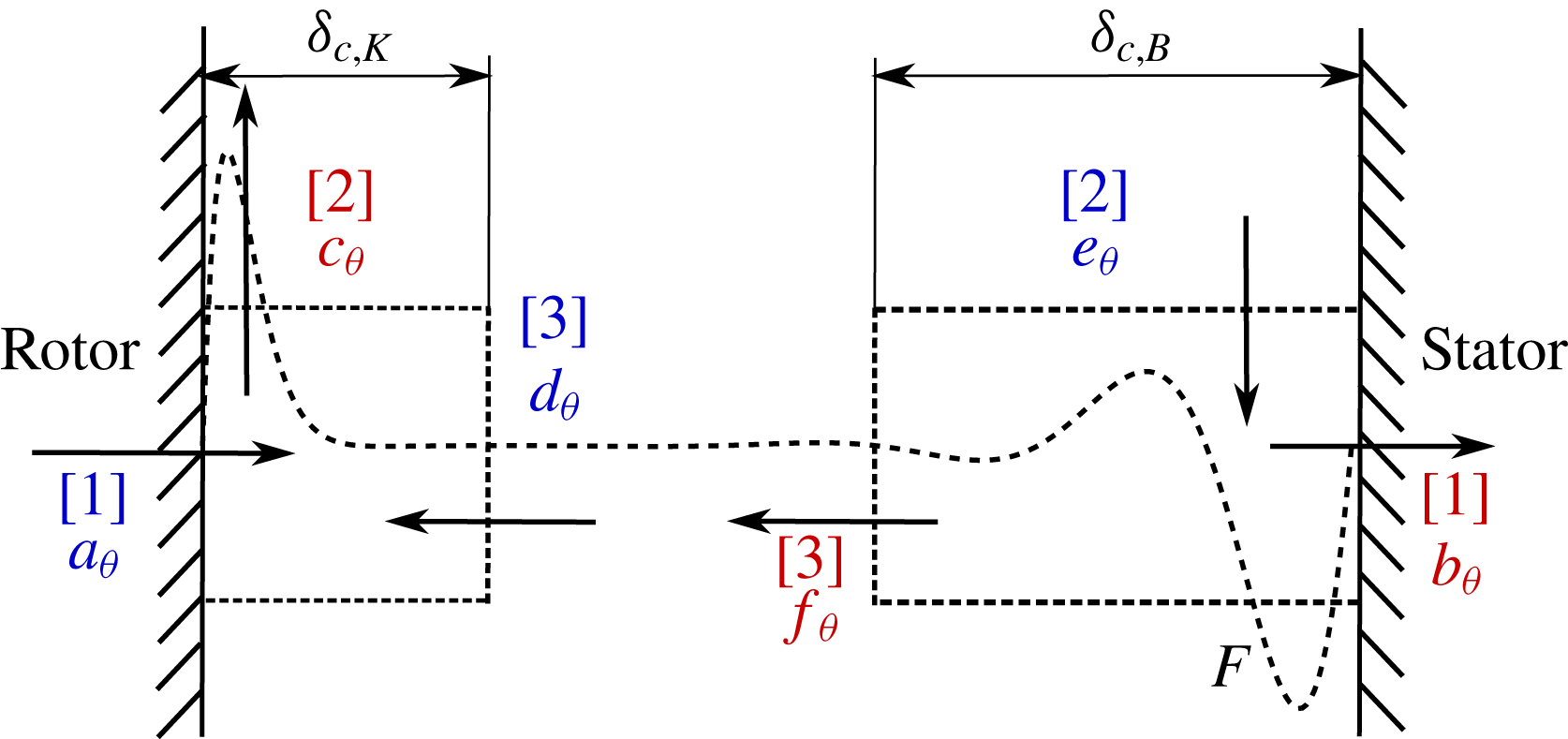
Angular momentum balance. The objective of this and the following section is to link the differential solutions with an integrated approach to the problem, which is frequently used in zero-dimensional models (Gärtner Reference Gärtner1998; Chew & Hills Reference Chew and Hills2013; Sun et al. Reference Sun, Amirante, Chew and Hills2016). Moreover, further insight can be gained by looking at the overall angular momentum and energy balance. The continuity equation, (2.6a ), and the momentum equation in the azimuthal direction, equation (2.6c ), can be combined to obtain the conservative form of (2.6c ),
 $$\begin{eqnarray}\frac{1}{Re_{s}}\frac{\unicode[STIX]{x2202}}{\unicode[STIX]{x2202}\unicode[STIX]{x1D709}}(G^{\prime })=4FG+\frac{1}{Re_{s}^{1/2}}\frac{\unicode[STIX]{x2202}}{\unicode[STIX]{x2202}\unicode[STIX]{x1D709}}(HG).\end{eqnarray}$$
Integrating (2.26) over a control volume defined from the wall to a distance well beyond the edge of the boundary layer,
 $\unicode[STIX]{x1D6FF}_{K}/s\gg Re_{s}^{-1/2}$
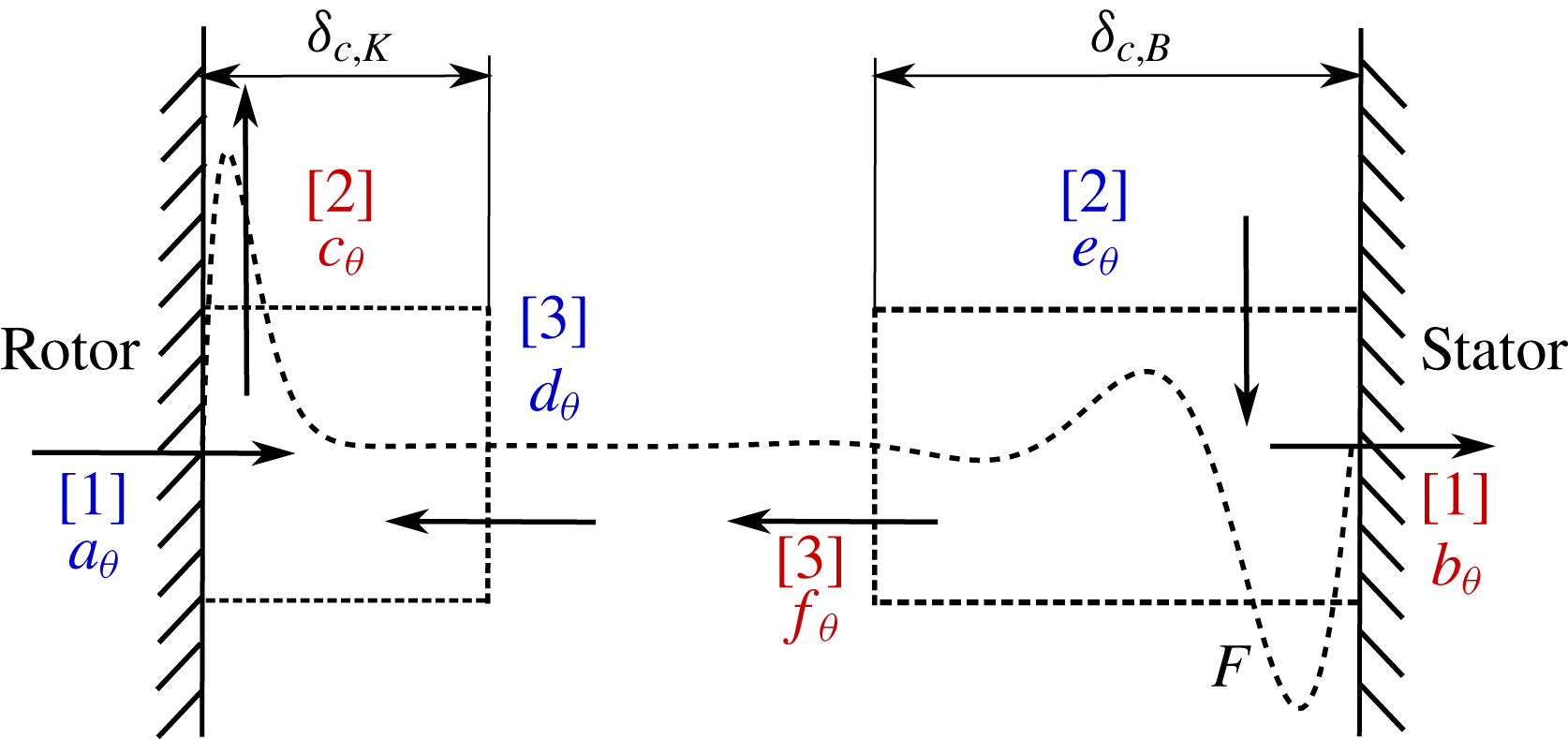
in the core region. The conservation of angular momentum in the overall domain can be separated into two independent control volumes, as shown in figure 5. Making use of the fact that in the core region
 $F_{core}=G_{core}^{\prime }=0,$
and at the wall
 $H_{wall}=0,$
the integral momentum equation becomes
 $$\begin{eqnarray}\underbrace{\left.\frac{1}{Re_{s}}G^{\prime }\right|_{rotor}}_{[1]}=-\underbrace{\int _{0}^{\unicode[STIX]{x1D6FF}_{K}}4F(\unicode[STIX]{x1D709})G(\unicode[STIX]{x1D709})\,\text{d}\unicode[STIX]{x1D709}}_{[2]}-\underbrace{{\displaystyle \frac{1}{Re_{s}^{1/2}}}H_{core}G_{core}}_{[3]}.\end{eqnarray}$$
The dimensionless shear stress at the walls can be expressed as
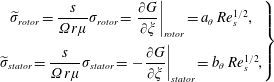 $$\begin{eqnarray}\left.\begin{array}{@{}c@{}}\widetilde{\unicode[STIX]{x1D70E}}_{rotor}={\displaystyle \frac{s}{\unicode[STIX]{x1D6FA}r\unicode[STIX]{x1D707}}}\unicode[STIX]{x1D70E}_{rotor}=\left.{\displaystyle \frac{\unicode[STIX]{x2202}G}{\unicode[STIX]{x2202}\unicode[STIX]{x1D709}}}\right|_{rotor}=a_{\unicode[STIX]{x1D703}}\,Re_{s}^{1/2},\\ \widetilde{\unicode[STIX]{x1D70E}}_{stator}={\displaystyle \frac{s}{\unicode[STIX]{x1D6FA}r\unicode[STIX]{x1D707}}}\unicode[STIX]{x1D70E}_{stator}=\left.-{\displaystyle \frac{\unicode[STIX]{x2202}G}{\unicode[STIX]{x2202}\unicode[STIX]{x1D709}}}\right|_{stator}=b_{\unicode[STIX]{x1D703}}\,Re_{s}^{1/2},\end{array}\right\}\end{eqnarray}$$
where
 $a_{\unicode[STIX]{x1D703}}$
and
 $b_{\unicode[STIX]{x1D703}}$
represent the universal non-dimensional shear stress in the rotor and stator, respectively. In the same line
 $f_{\unicode[STIX]{x1D703}}=d_{\unicode[STIX]{x1D703}}=H_{core}G_{core},$
and
 $c_{\unicode[STIX]{x1D703}}$
is defined as
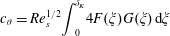 $$\begin{eqnarray}c_{\unicode[STIX]{x1D703}}=Re_{s}^{1/2}\int _{0}^{\unicode[STIX]{x1D6FF}_{K}}4F(\unicode[STIX]{x1D709})G(\unicode[STIX]{x1D709})\,\text{d}\unicode[STIX]{x1D709}\end{eqnarray}$$
in the rotor. The equivalent integral in the stator defines
 $e_{\unicode[STIX]{x1D703}}$
.
Constant values for the non-dimensional conservation of angular momentum.

Figure 5 outlines the tangential momentum equilibrium in a rotor–stator cavity identifying the terms of (2.27), whereas table 1 provides the actual values of the constants used in this figure. The tangential momentum generated by rotation of the rotor,
 $a_{\unicode[STIX]{x1D703}}$
, is convected outwards,
 $c_{\unicode[STIX]{x1D703}}$
, together with the azimuthal momentum convected in the core from the stator to the rotor,
 $d_{\unicode[STIX]{x1D703}}$
. This actually means that
 $c_{\unicode[STIX]{x1D703}}=a_{\unicode[STIX]{x1D703}}+d_{\unicode[STIX]{x1D703}}$
. Analogously, in the stator, momentum is radially convected inwards,
 $e_{\unicode[STIX]{x1D703}}$
, convected axially to the rotor,
 $d_{\unicode[STIX]{x1D703}}$
, and transmitted partially to the stator,
 $b_{\unicode[STIX]{x1D703}}$
. Momentum balances dictate that
 $e_{\unicode[STIX]{x1D703}}=b_{\unicode[STIX]{x1D703}}+d_{\unicode[STIX]{x1D703}}$
. It is interesting to note that since
 $a_{\unicode[STIX]{x1D703}}\neq b_{\unicode[STIX]{x1D703}}$
, the torque of the rotor is not fully transmitted to the stator.
Energy balance. Analogously to the azimuthal momentum equation, the continuity equation (2.6a ) can be combined with the energy equations (2.14) and (2.15), to obtain the corresponding energy equations in conservative form:
 $$\begin{eqnarray}\displaystyle \frac{1}{PrRe_{s}}\frac{\unicode[STIX]{x2202}}{\unicode[STIX]{x2202}\unicode[STIX]{x1D709}}(\tilde{T}_{0}^{\prime }) & = & \displaystyle 4F\tilde{T}_{0}+\frac{1}{Re_{s}^{1/2}}\frac{\unicode[STIX]{x2202}}{\unicode[STIX]{x2202}\unicode[STIX]{x1D709}}(H\tilde{T}_{0}),\end{eqnarray}$$
 $$\begin{eqnarray}\displaystyle \frac{1}{PrRe_{s}}\frac{\unicode[STIX]{x2202}}{\unicode[STIX]{x2202}\unicode[STIX]{x1D709}}(\tilde{T}_{2}^{\prime }) & = & \displaystyle 4F\tilde{T}_{2}+\frac{1}{Re_{s}^{1/2}}\frac{\unicode[STIX]{x2202}}{\unicode[STIX]{x2202}\unicode[STIX]{x1D709}}(H\tilde{T}_{2})-\frac{Ec}{Re_{s}}(G^{\prime 2}+F^{\prime 2}).\end{eqnarray}$$
 $\unicode[STIX]{x1D6FF}_{T}/s\gg Pr^{-1/2}Re_{s}^{-1/2}$
in the core region. The conservation of energy in the whole domain can be split into two independent control volumes. Making use of the fact that, in the core region
 $F_{core}=T_{0,core}=T_{0,core}^{\prime }=T_{2,core}^{\prime }=0,$
and at the wall
 $H_{wall}=0,$
the two integral energy equations become
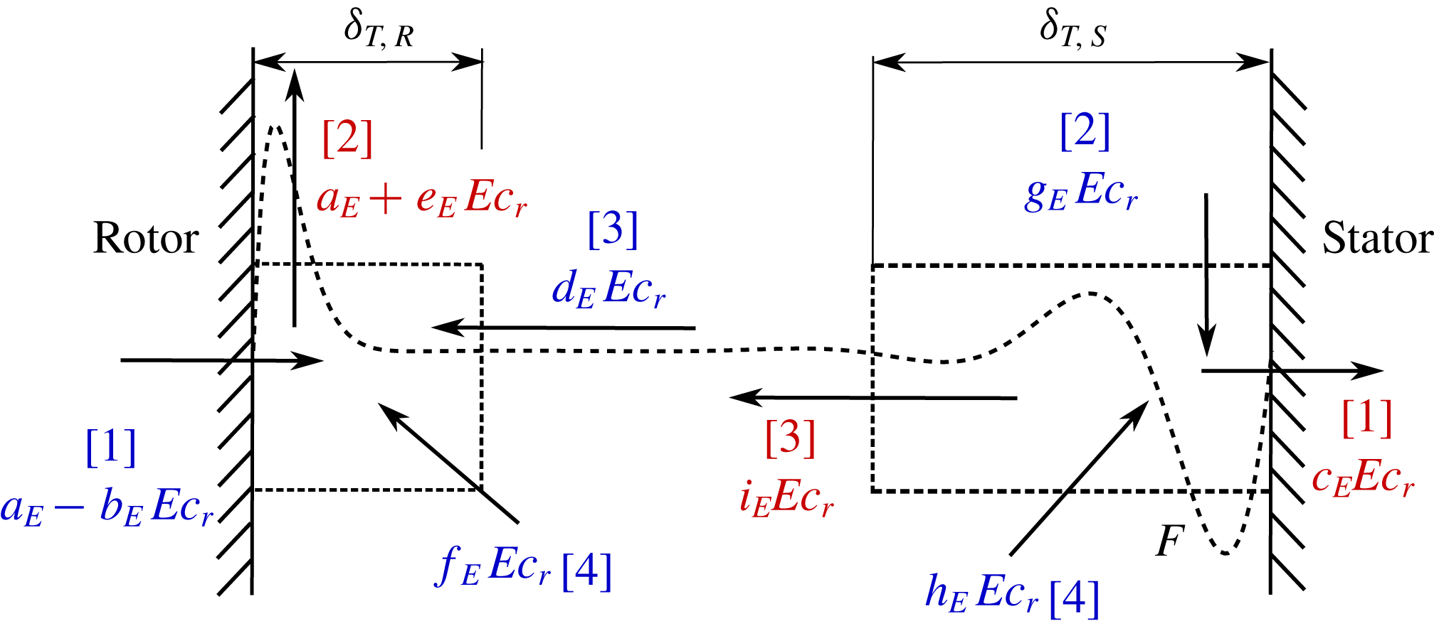
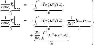 $$\begin{eqnarray}\left.\begin{array}{@{}rcl@{}}\underbrace{\left.{\displaystyle \frac{1}{PrRe_{s}}}\widetilde{T}_{0}^{\prime }\right|_{rotor}}_{[1]} & = & -\underbrace{\displaystyle \int _{0}^{\unicode[STIX]{x1D6FF}_{T}}4\widetilde{T}_{0}(\unicode[STIX]{x1D709})F(\unicode[STIX]{x1D709})\,\text{d}\unicode[STIX]{x1D709}}_{[2]},\\ \underbrace{\left.{\displaystyle \frac{1}{PrRe_{s}}}\widetilde{T}_{2}^{\prime }\right|_{rotor}}_{[1]} & = & -\underbrace{\displaystyle \int _{0}^{\unicode[STIX]{x1D6FF}_{T}}4\widetilde{T}_{2}(\unicode[STIX]{x1D709})F(\unicode[STIX]{x1D709})\,\text{d}\unicode[STIX]{x1D709}}_{[2]}-\underbrace{{\displaystyle \frac{1}{Re_{s}^{1/2}}}H_{core}\widetilde{T}_{2,core}}_{[3]}\\ & & +\,\underbrace{{\displaystyle \frac{Ec}{Re_{s}}}\displaystyle \int _{0}^{\unicode[STIX]{x1D6FF}_{T}}(G^{\prime 2}+F^{\prime 2})\,\text{d}\unicode[STIX]{x1D709}}_{[4]}.\end{array}\right\}\end{eqnarray}$$
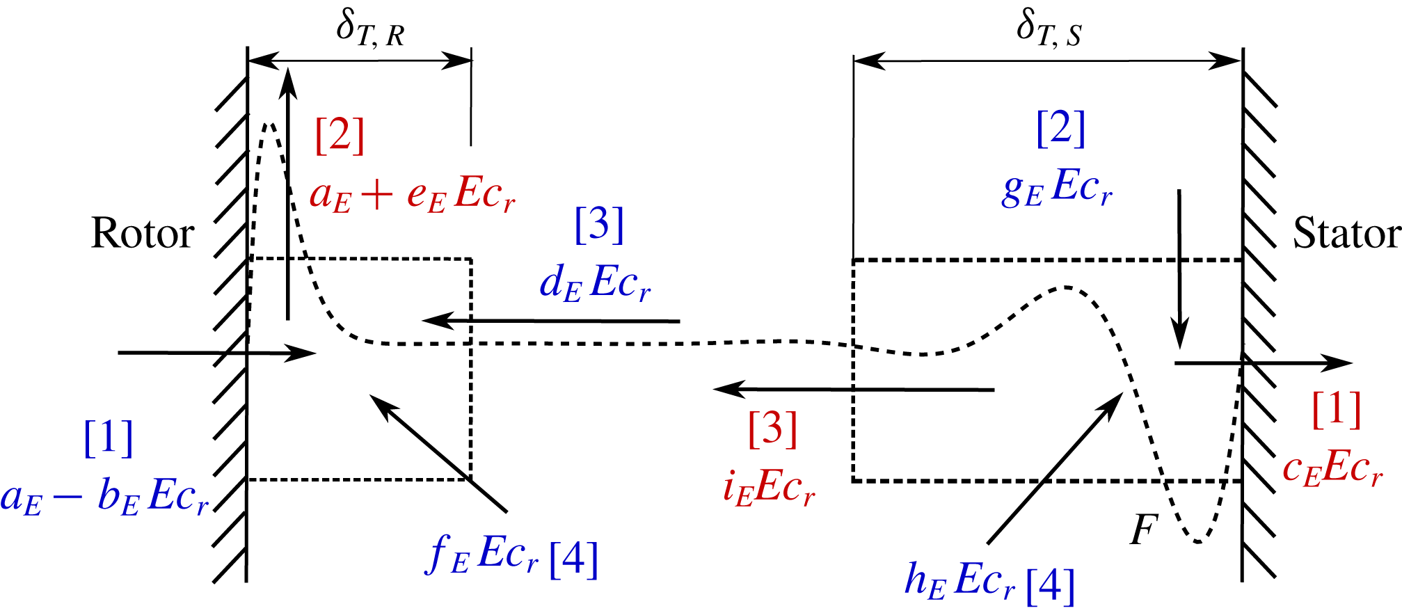
Figure 6 sketches (2.31) in graphical form. Heat flux is non-dimensionalised using
 $q_{ref}=k(T_{R}-T_{S})/s$
and renormalised with
 $Re_{s}^{1/2}$
to absorb the dependence on the Reynolds number. The non-dimensional heat fluxes at the rotor and stator are then
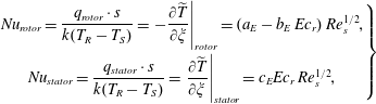 $$\begin{eqnarray}\left.\begin{array}{@{}c@{}}Nu_{rotor}={\displaystyle \frac{q_{rotor}\cdot s}{k(T_{R}-T_{S})}}=\left.-{\displaystyle \frac{\unicode[STIX]{x2202}\widetilde{T}}{\unicode[STIX]{x2202}\unicode[STIX]{x1D709}}}\right|_{rotor}=(a_{E}-b_{E}\,Ec_{r})\,Re_{s}^{1/2},\\ Nu_{stator}={\displaystyle \frac{q_{stator}\cdot s}{k(T_{R}-T_{S})}}=\left.{\displaystyle \frac{\unicode[STIX]{x2202}\widetilde{T}}{\unicode[STIX]{x2202}\unicode[STIX]{x1D709}}}\right|_{stator}=c_{E}Ec_{r}\,Re_{s}^{1/2},\end{array}\right\}\end{eqnarray}$$
where the explicit dependence on
 $Re_{s}^{1/2}$
can be seen. This definition is consistent with the classical definition of the Nusselt number based on the gap. All the terms affected by the
 $Ec_{r}$
have their origin in the quadratic terms of the energy equation. The rest of the terms of table 2 are defined as
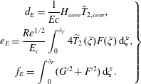 $$\begin{eqnarray}\left.\begin{array}{@{}c@{}}d_{E}={\displaystyle \frac{1}{Ec}}H_{core}\tilde{T}_{2,core},\\ e_{E}={\displaystyle \frac{Re^{1/2}}{E_{c}}}\displaystyle \int _{0}^{\unicode[STIX]{x1D6FF}_{T}}4\widetilde{T}_{2}(\unicode[STIX]{x1D709})F(\unicode[STIX]{x1D709})\,\text{d}\unicode[STIX]{x1D709},\\ f_{E}=\displaystyle \int _{0}^{\unicode[STIX]{x1D6FF}_{T}}(G^{\prime 2}+F^{\prime 2})\,\text{d}\unicode[STIX]{x1D709}.\end{array}\right\}\end{eqnarray}$$
Renormalised non-dimensional heat flux balance (
 $qs/k(T_{R}-T_{s})Re_{s}^{1/2}$
).
Constant values for the non-dimensional energy budget for
 $Pr=0.71$
.

The rest of the constants in table 2,
 $c_{E}$
,
 $i_{E}$
,
 $h_{E}$
and
 $g_{E}$
, are the corresponding parts in the stator of
 $b_{E}$
,
 $d_{E}$
,
 $f_{E}$
and
 $e_{E}$
, respectively. As can be seen in figure 6, viscous dissipation has a determinant effect on the temperature near the rotor wall. In addition, we can estimate the value of the temperature at the core region using the energy balance previously studied. Assuming the conservation of mass flow over the whole domain, the dimensionless axial velocity at the core region can be estimated as
 $$\begin{eqnarray}H_{core}=1-\unicode[STIX]{x1D6FD}^{2}H_{B\ddot{o} \mathit{dewadt}},\end{eqnarray}$$
keeping in mind that
 $H_{B\ddot{o} \mathit{dewadt}}=1.35$
(Bödewadt Reference Bödewadt1940). On the other hand, using the numerical results of the energy balance shown in figure 6, we can derive
 $d_{E},$
and making use of the expression of the axial convection term in (2.33), we can estimate
 $\tilde{T}_{core}$
as a function of the dimensionless axial velocity at the core region as follows, using the constant values given in table 2:
 $$\begin{eqnarray}\widetilde{T}_{core}=\frac{d_{E}\,Ec_{r}}{H_{core}}.\end{eqnarray}$$
Substituting (2.34) into (2.35) we can obtain an estimate for
 $\tilde{T}_{core}$
as a function of the swirl factor and the Eckert number:
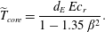 $$\begin{eqnarray}\widetilde{T}_{core}=\frac{d_{E}\,Ec_{r}}{1-1.35\,\unicode[STIX]{x1D6FD}^{2}}.\end{eqnarray}$$
Note that the radial variation of the temperature,
 $\hat{T}_{2}$
, is not controlled by the temperature difference between the rotor and the stator, since actually
 $T_{2R}-T_{2S}=0$
. The temperature in the core,
 $\hat{T}_{core}$
, is controlled by viscous heating in the stator and the subsequent convection from the stator to the rotor; windage heating contributes to increasing the temperature at the core region. The increment of temperature due to the dissipation can be estimated as
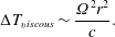 $$\begin{eqnarray}\unicode[STIX]{x0394}T_{viscous}\sim \frac{\unicode[STIX]{x1D6FA}^{2}r^{2}}{c}.\end{eqnarray}$$
2.2.2 Transient solutions
Instantaneous spin-up. A previous study by Owen, Pincombe & Rogers (Reference Owen, Pincombe and Rogers1985) demonstrated that the steady solutions obtained with the present formulation were able to reproduce experimental results with reasonable agreement. In the present work, emphasis is placed on the transient evolution of a still fluid when the rotor is impulsively started. The same set of dimensionless parameters used in the stationary case has been kept. Although the initial and final states of the fluid are relatively simple and have been well studied in the past, the transient state is non-trivial because it involves the time-dependent evolution of a coupled convective and diffusive mechanical system.
Let us consider again the dimensionless circumferential momentum equation:
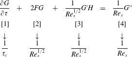 $$\begin{eqnarray}\begin{array}{@{}ccccccc@{}}\displaystyle {\displaystyle \frac{\unicode[STIX]{x2202}G}{\unicode[STIX]{x2202}\unicode[STIX]{x1D70F}}} & + & 2FG & + & {\displaystyle \frac{1}{Re_{s}^{1/2}}}G^{\prime }H & = & {\displaystyle \frac{1}{Re_{s}}}G^{\prime \prime }\\ \displaystyle \text{ }[1] & & [2] & & [3] & & [4]\\ \displaystyle \downarrow & & \downarrow & & \downarrow & & \downarrow \\ \displaystyle {\displaystyle \frac{1}{\unicode[STIX]{x1D70F}_{c}}} & & {\displaystyle \frac{1}{Re_{s}^{1/2}}} & & {\displaystyle \frac{1}{Re_{s}^{1/2}}} & & {\displaystyle \frac{1}{Re_{s}}}\end{array}\end{eqnarray}$$
In the core region,
 $v_{\unicode[STIX]{x1D703}}\sim \unicode[STIX]{x1D6FA}r$
, and therefore
 $G\sim \mathit{O}(1)$
, the radial velocity is very small,
 $v_{r}\ll \unicode[STIX]{x1D6FA}r$
. Actually, in accordance with the dimensionless continuity equation, equation (2.6a
),
 $F\sim Re_{s}^{-1/2}$
, and therefore both convective terms of (2.38) (terms [2] and [3]) are of order
 $Re_{s}^{-1/2}$
, and then much larger than the diffusive term [4], which is of order
 $Re^{-1}$
. The time derivative is of the same order as the convective terms [1]–[2] or [3] when
 $\unicode[STIX]{x1D70F}_{c}=\unicode[STIX]{x1D70F}_{r}\sim Re_{s}^{1/2}$
. Physically, this is the time needed for a fluid particle to move from the stator to the rotor,
 $\unicode[STIX]{x1D70F}_{r}.$
This can be noticed by realising that the characteristic velocity in the axial direction is
 $v_{zc}\sim (\unicode[STIX]{x1D708}\unicode[STIX]{x1D6FA})^{1/2},$
and therefore
 $$\begin{eqnarray}\unicode[STIX]{x1D70F}_{r}=\unicode[STIX]{x1D6FA}t_{r}=\unicode[STIX]{x1D6FA}\left(\frac{s}{v_{zc}}\right)\sim \frac{\unicode[STIX]{x1D6FA}s}{(\unicode[STIX]{x1D708}\unicode[STIX]{x1D6FA})^{1/2}}=Re_{s}^{1/2}.\end{eqnarray}$$
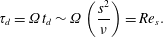
The dimensionless diffusive time,
 $\unicode[STIX]{x1D70F}_{d}$
, corresponds to the time taken by the diffusion to transport angular momentum in the axial direction. This would be the characteristic time if
 $H$
, i.e. the axial velocity, were strictly zero. In this case, the balance between the temporal derivatives and the viscous terms (term [4] in (2.38)) would yield
 $\unicode[STIX]{x1D70F}_{c}=\unicode[STIX]{x1D70F}_{d}\sim Re_{s}$
. This conclusion can be directly obtained by non-dimesionalising the diffusion time
 $$\begin{eqnarray}\unicode[STIX]{x1D70F}_{d}=\unicode[STIX]{x1D6FA}t_{d}\sim \unicode[STIX]{x1D6FA}\left(\frac{s^{2}}{\unicode[STIX]{x1D708}}\right)=Re_{s}.\end{eqnarray}$$
There is a third characteristic time, which is the time taken by the diffusion to form the disk boundary layer,
 $t_{BL}\sim \unicode[STIX]{x1D6FF}_{c}^{2}/\unicode[STIX]{x1D708}=\unicode[STIX]{x1D6FA}^{-1}$
. This was the time taken to non-dimesionalise the equations, and hence,
 $\unicode[STIX]{x1D70F}_{BL}\sim \mathit{O}(1)$
.
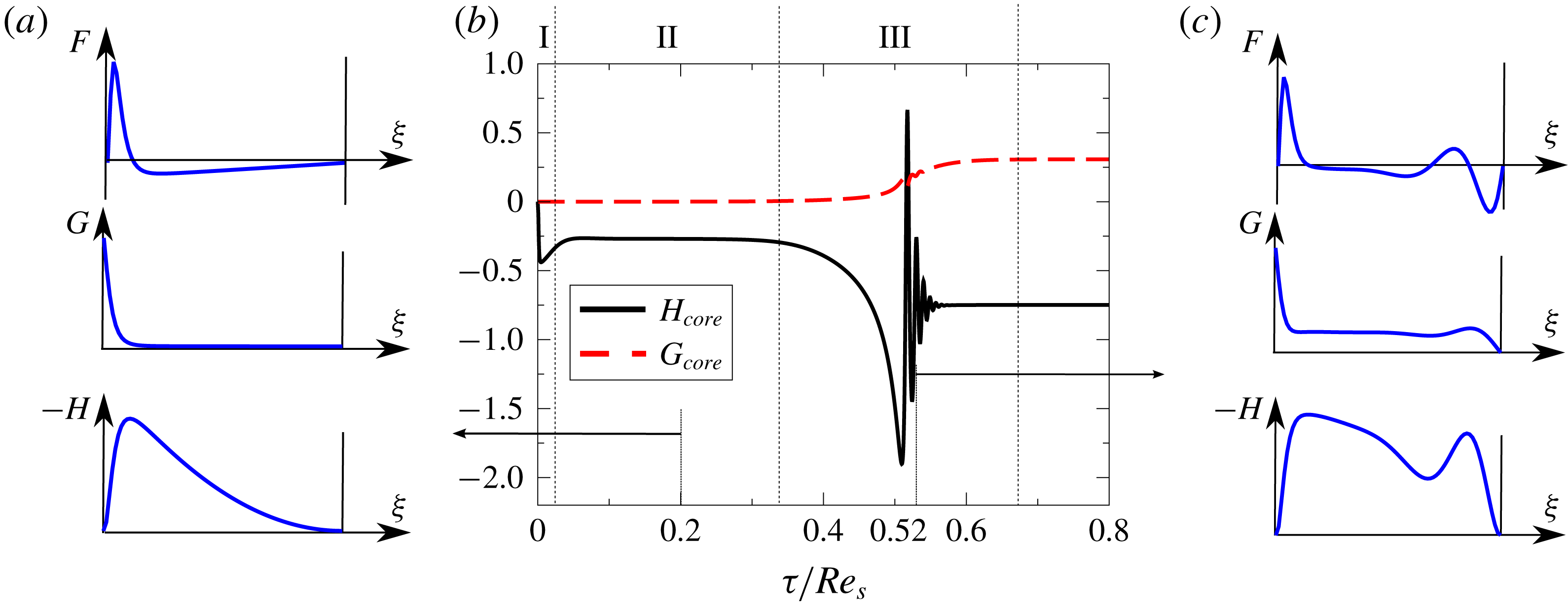
Dimensionless velocity components at the midpoint of the core region (
 $\unicode[STIX]{x1D709}=0.5$
) as a function of dimensionless time scaled with the diffusive time at
 $Re_{s}=2000$
for a disk impulsively started from rest (b). Velocity fields at (a)
 $\unicode[STIX]{x1D70F}=0.2Re_{s}$
(stage II) and (c)
 $\unicode[STIX]{x1D70F}=0.52Re_{s}$
(stage III).
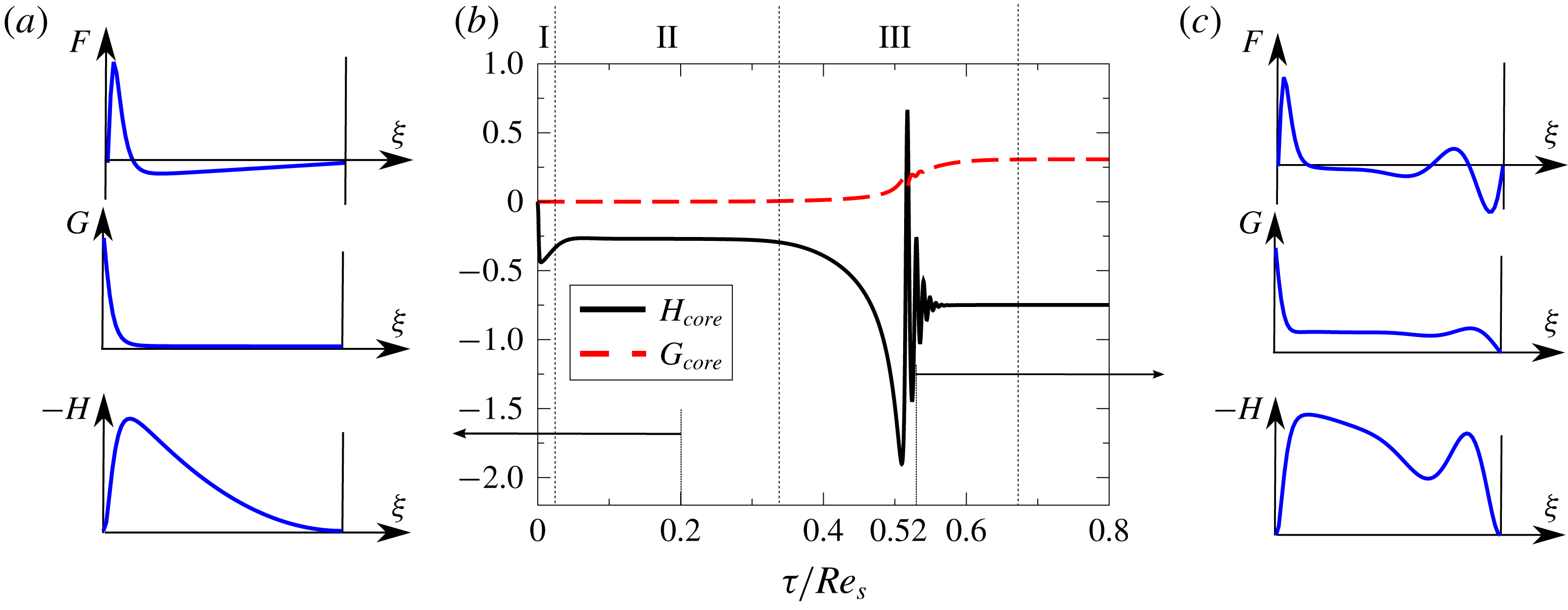
The existence of three different characteristic times gives rise to three distinct phases of motion, namely, the rapid formation of the von Kármán boundary layer (stage I) where a quasi-stationary Stewartson-type of flow is created, a spinning-up (stage II) process by which the non-viscous core acquires its angular momentum, and finally the formation of a Batchelor-type flow field, once Bödewadt’s boundary layer is created at the stator and the swirl at the core is adjusted, balancing the rotor and stator boundary layers (stage III).
Figure 7 displays the time evolution of the axial and circumferential velocities for the impulsive start from rest (
 $F_{0}=G_{0}=H_{0}=0$
at
 $\unicode[STIX]{x1D70F}=0$
) of one of the disks of an infinite rotor–stator cavity at
 $Re_{s}=2000$
, computed with the numerical scheme previously outlined. At
 $\unicode[STIX]{x1D70F}=0$
, the rotor is impulsively set in motion, resulting in the very rapid formation of a Stewartson-type flow. This phase (stage I) can be seen as the development of a von Kármán boundary layer in a free disk, which is independent of
 $Re_{s}$
. The characteristic time of stage I is of order unity,
 $\unicode[STIX]{x1D70F}_{I}\sim \mathit{O}(1)$
. A von Kármán boundary layer is created in the rotating disk in which the azimuthal velocity decreases from the disk rotational velocity at the wall to the core velocity, which at this initial state is zero.
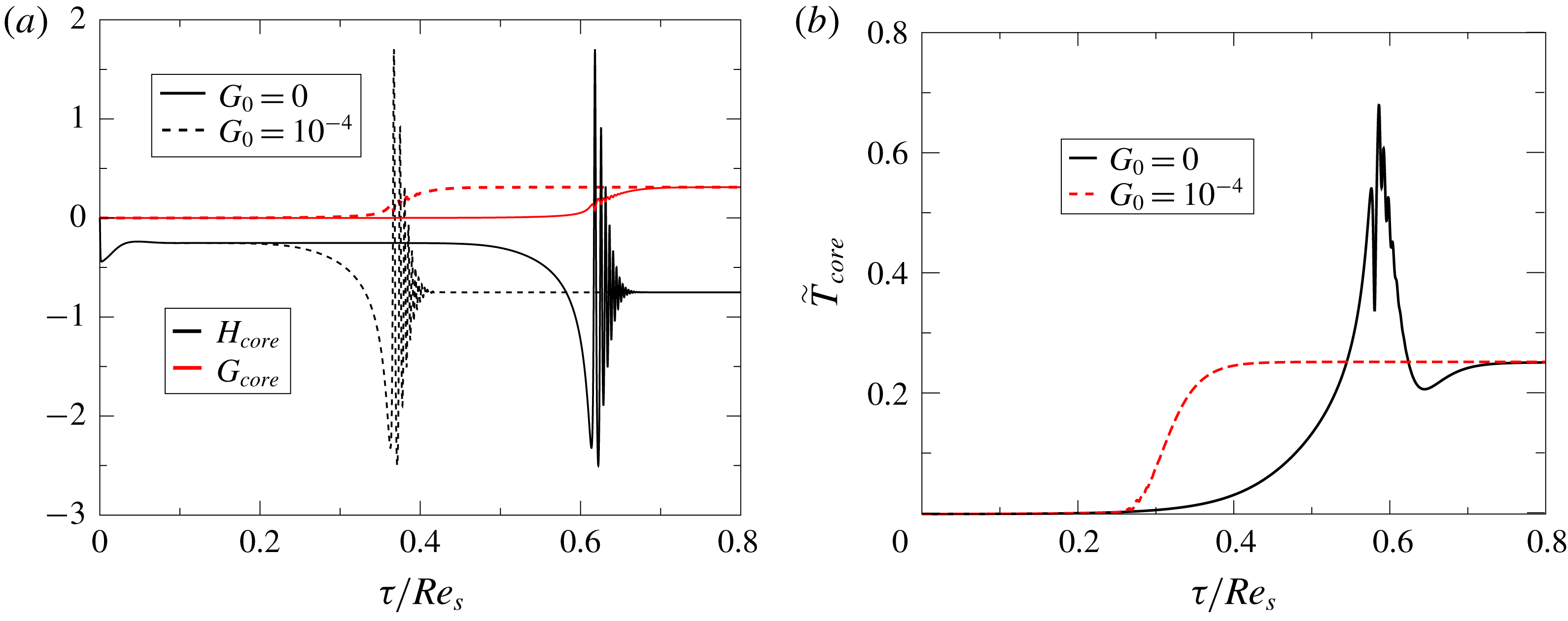
The subsequent stage II is highly sensitive to the details of the initial condition of the circumferential velocity. If
 $G_{0}$
is strictly zero at
 $\unicode[STIX]{x1D70F}=0$
, then the azimuthal velocity can only increase by diffusion from the disk wall, since the convective terms, [2] and [3], in (2.38) are strictly zero in the core region. The axial velocity,
 $H$
, constant and negative in the core region, is responsible for feeding the radial boundary layer created in the disk; however, it can only transport fluid with zero tangential momentum. This effectively means that the tangential momentum created by the disk is convected back to the disk; as a consequence the tangential momentum in the core region can only be increased by diffusion, and hence this stage lasts for a time
 $\unicode[STIX]{x1D70F}_{II}\sim Re_{s}$
, which is very long. This can be seen in figure 7(a) where a Stewartson-like velocity profile is observed in this stage.
The quasi-steady Stewartson-type flow rapidly changes after
 $\unicode[STIX]{x1D70F}\simeq 0.34Re_{s}$
: see figure 7(b). At this point, the tangential momentum, transported by diffusion from the disk, is radially convected inwards because the radial velocity in the core region of the Stewartson flow is negative. Since in the inviscid core region
 $rv_{\unicode[STIX]{x1D703}}$
is constant along the pathlines, a reduction in radius automatically implies an increase in the dimensionless circumferential velocity,
 $G$
. From a mathematical point of view the term [2] of (2.38) is no longer zero and triggers the exponential creation of circumferential momentum in a time
 $\unicode[STIX]{x1D70F}_{d}=\unicode[STIX]{x1D70F}_{II}\sim Re_{s}$
. Some researchers (van Eeten et al.
Reference van Eeten, van der Schaaf, van Heijst and Schouten2013) describe this phenomenon as an instability of the Stewartson flow.
Once the core of the disk begins to rotate as a rigid body, a Bödewadt’s boundary layer is created in the stationary disk, in a time of the order of the diffusive time of the boundary layer,
 $\unicode[STIX]{x1D70F}_{BL}\sim \mathit{O}(1)$
. This can be seen in figure 7(c) where a Batchelor-type flow is depicted. However, during this stage III, the von Kármán and the Bödewadt boundary layers are not in equilibrium since they are not symmetric. For a given arbitrary swirl factor of the core,
 $\unicode[STIX]{x1D6FD}$
, firstly, the tangential momentum created in the core by both boundary layers is not in equilibrium, and secondly, the fluid ingested by the disk and egressed by the stationary disk does not match either. This global balance is established by convecting tangential momentum and mass from the stationary to the rotating disk in a time of the order of the residence time of the axial velocity of the core,
 $\unicode[STIX]{x1D70F}_{r}=\unicode[STIX]{x1D70F}_{III}\sim Re_{s}^{1/2}$
. The axial mass flow ingested by the disk during stage II of the process is smaller than that egressed by the stator once Bödewadt’s boundary is formed and the final steady state is reached (see figure 7
b). Since the flow is incompressible, this mismatch gives rise to a steep change in the axial velocity at
 $\unicode[STIX]{x1D70F}\simeq 0.52Re_{s}$
, in figure 7(c), and inertial waves are clearly seen in figure 7(b). We have tracked the duration of the spikes seen during the third phase of the transient stage, and we have also verified that its characteristic time scales as
 $\unicode[STIX]{x1D70F}_{c}\sim Re_{s}^{1/2}$
.
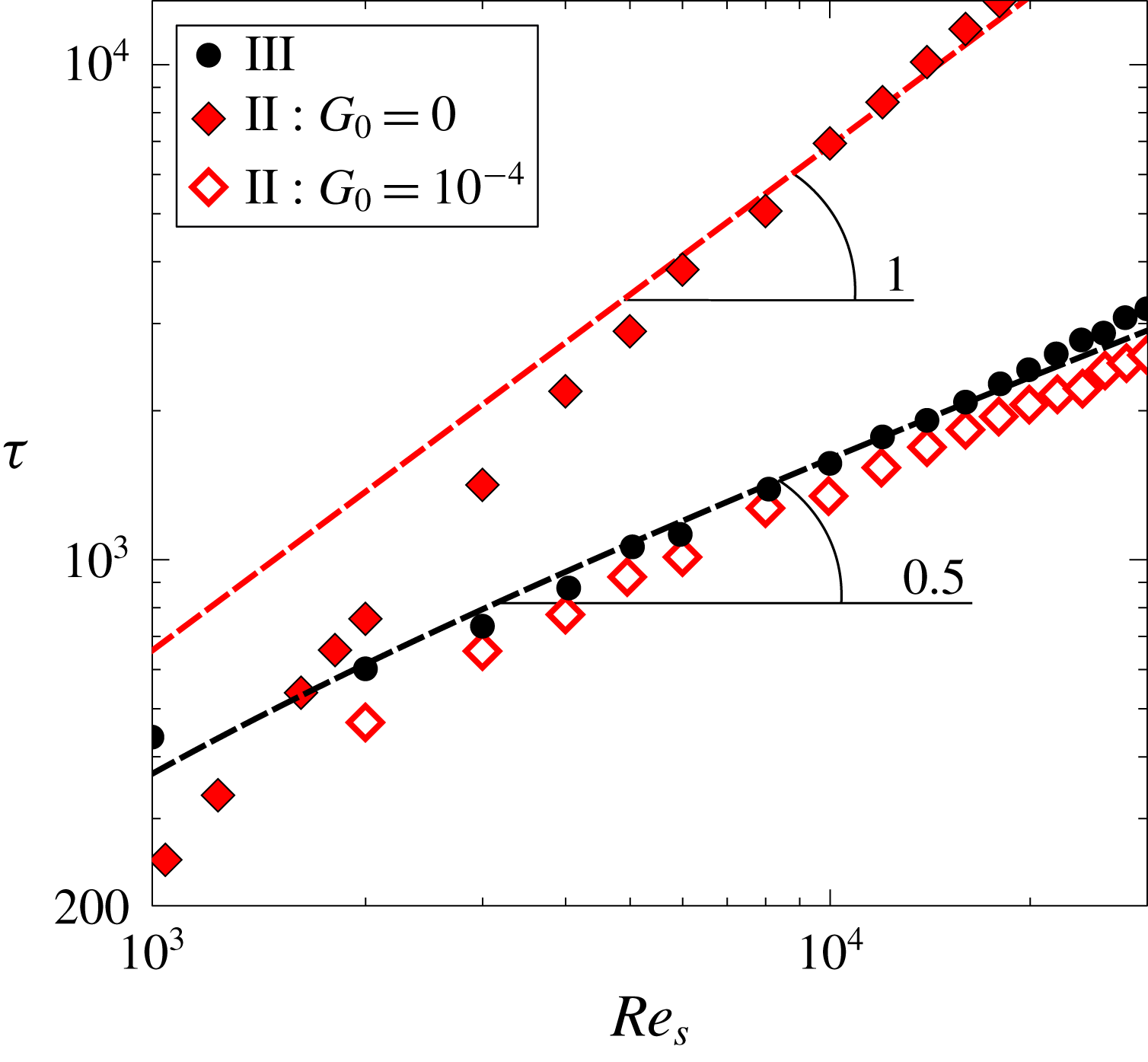
Dimensionless time of stages II and III for different initial conditions.
We have solved the problem for different
 $Re_{s}$
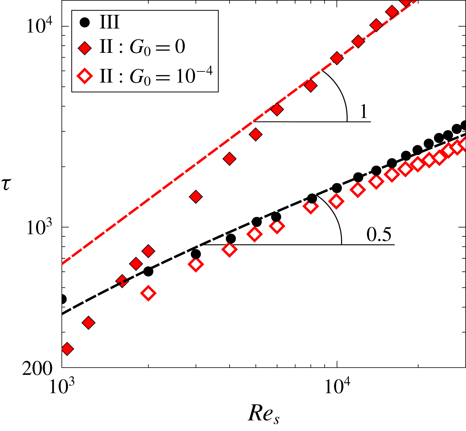
and identified manually stages II and III. Figure 8 displays the duration of stage II (♦) and stage III (●) as a function of the Reynolds number. The slopes 1 and 0.5 are plotted to help the reader to draw their own conclusions. It is clearly seen that when the disk is impulsively started from rest, and the three components of the fluid velocity are strictly zero, the characteristic times of the stage II and III of the problem scale with
 $Re_{s}$
and
 $Re_{s}^{1/2}$
, respectively. These trends are more easily seen at the largest Reynolds numbers.
Stage II of the transient changes dramatically if the dimensionless circumferential velocity is initialised to a small value. Figure 8 displays the duration of stage II when
 $G$
is initialised to
 $10^{-4}$
(♢). It can be seen that, in this case, stage II is bypassed, and only the convective part of the process, which takes place in times of the order of
 $Re_{s}^{1/2}$
, can be seen. The starting process described when the fluid velocity is strictly zero at
 $\unicode[STIX]{x1D70F}=0$
, cannot be seen in practice in real engines, since frequently analyses are focused on the acceleration of the engine from idle to maximum take-off. The flow in the initial stage is already rotating (
 $G_{0}\neq 0$
), and hence the diffusive stage is bypassed. Idle rotational speed is approximately 10 % of maximum take-off rotational speed so that
 $G_{0}$
is actually much greater than
 $10^{-4}$
. Even if the disk is started from rest, there are always velocity perturbations associated either with the ventilation of the system or natural convection, if the engine is restarted, which are at least of the order of
 $10^{-3}$
. Hence our understanding is that the diffusive part of the process is always bypassed in realistic cases and it is not relevant.
It has been reported (Lopez et al.
Reference Lopez, Marques, Rubio and Avila2009) that the spin-up and spin-down processes give rise to axisymmetric circular waves inside Bödewadt’s boundary layer. These radial variations cannot be captured by the similarity analysis presented here, which prescribes a linear variation of the velocity with the radius. Fortunately, these perturbations die out in very short times,
 $\unicode[STIX]{x1D70F}=\mathit{O}(1)$
. This actually means that this very short transient, although not seen in the solutions, hardly affects the global transient behaviour of the cavity, whose characteristic time is much longer.
Transient evolution scaled with the diffusive time of the axial and circumferential dimensionless velocities (a) and dimensionless temperature (b) at the midpoint of the core region (
 $\unicode[STIX]{x1D709}=0.5$
) when the cavity is initially at rest (
 $G_{0}=0$
at
 $\unicode[STIX]{x1D70F}=0$
) and when it is uniformly initialised (
 $G_{0}=10^{-4}$
at
 $\unicode[STIX]{x1D70F}=0$
), at
 $Re_{s}=4000$
,
 $Pr=0.71$
,
 $Ec_{r}=1$
.
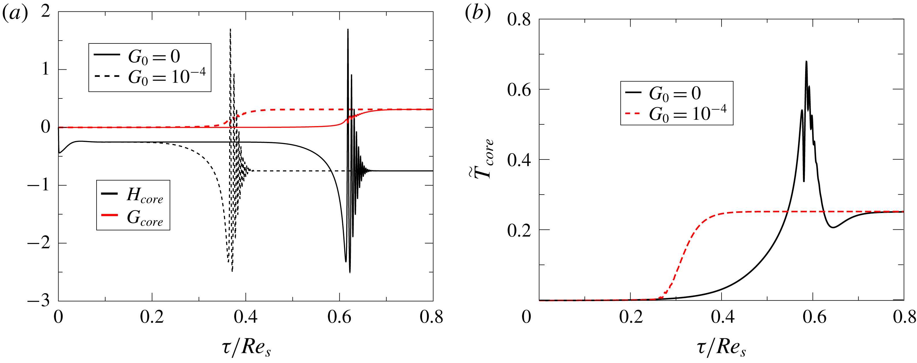
Figures 9(a) and 9(b) compare the evolution, for the same
 $Re_{s}$
, of the velocity and temperature fields in the core midpoint for two different initial conditions,
 $G_{0}=0$
and
 $G_{0}=10^{-4}$
. It is clearly seen that the final state is reached much earlier when the flow is started up with a fairly small perturbation than when the fluid is initially at rest. It can be concluded that, for
 $G_{0}=10^{-4}$
, the global dimensionless time evolution can be estimated as
 $$\begin{eqnarray}\unicode[STIX]{x1D70F}_{t}\simeq \unicode[STIX]{x1D70F}_{I}+\unicode[STIX]{x1D70F}_{II}+\unicode[STIX]{x1D70F}_{III}\propto Re_{s}^{1/2}.\end{eqnarray}$$
Usually, heat transfer analyses of the start-up process of a gas turbine assume that the flow is quasi-stationary with respect to the solid to avoid computing a very long transient stage, which can become unaffordable from a computational point of view. However, we will show that there are analytical indications that demonstrate that this might not necessarily be the case.
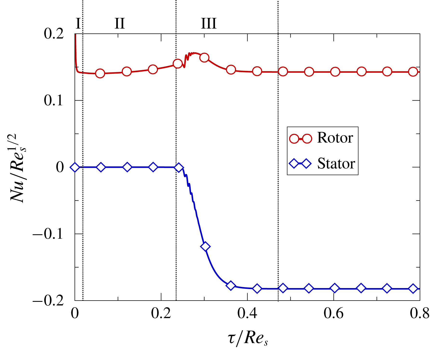
Transient evolution scaled with the diffusive time of the renormalised Nusselt number (
 $Nu/Re_{s}^{1/2}$
) at the stator and rotor with
 $G_{0}=10^{-4}$
, at
 $Re_{s}=4000$
,
 $Pr=0.71$
,
 $Ec_{r}=1$
.
The initial temperature of the fluid is assumed to be uniform and identical to that of the stator,
 $T_{i}(\unicode[STIX]{x1D709})=T_{S}$
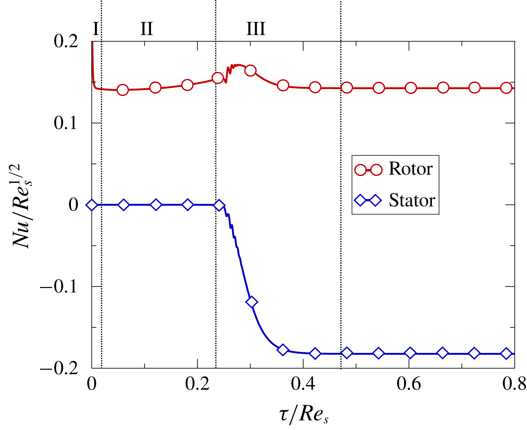
. We now study the time-dependent evolution of the temperature field, when the disk is impulsively started and the fluid is at rest. As is shown in the time-dependent evolution of
 $Nu_{rotor}$
in figure 10, the thermal boundary layer at the rotor is nearly instantaneously created (stage I), in a dimensionless time of the order of unity, reaching a quasi-steady value of the heat flux at the rotor. Once the thermal boundary layer at the rotor has been created,
 $\widetilde{T}_{0}$
remains constant in the whole domain, and it is identical to that shown in figure 4(b) for the stationary case. The non-dimensional heat flux in the rotor,
 $Nu_{rotor}$
, is constant and equal to that of the steady solution, for
 $\unicode[STIX]{x1D70F}\gg 1$
(stages II and III).
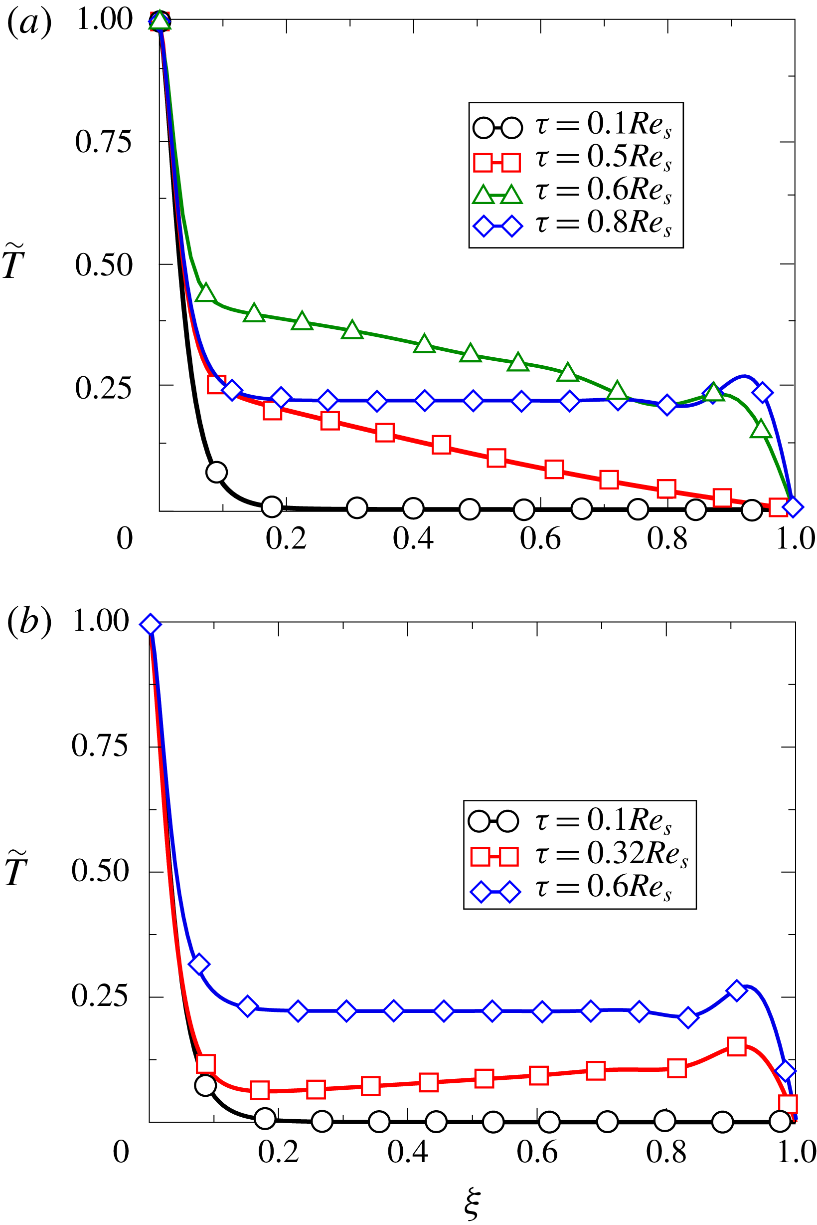
Dimensionless temperature field with
 $G_{0}=0$
(a) and
 $G_{0}=10^{-4}$
(b) at different dimensionless times for the case
 $Re_{s}=4000$
,
 $Pr=0.71$
,
 $Ec_{r}=1$
.
The time-dependent evolution of the temperature field separating the contribution of
 $\widetilde{T}_{0}$
and
 $\widetilde{T}_{2}$
, is studied in the following. The development of the temperature
 $\widetilde{T}_{0}$
can be studied from (2.14). Following the same argument as for the conservation of angular momentum in the azimuthal direction (2.6c
), it can be noticed that there is no term in (2.14) which can create an exponential growth of the temperature field and the contribution of
 $\tilde{T}_{0}$
to the temperature field is restricted to a narrow region in the vicinity of the rotor. In stage II, the temperature at the core region, which is solely due to the contribution of
 $\tilde{T}_{2}$
, increases due to the heating associated with the viscous dissipation term
 $Ec/Re_{s}(G^{\prime 2}+F^{\prime 2})$
in (2.15). The linear profile of
 $F$
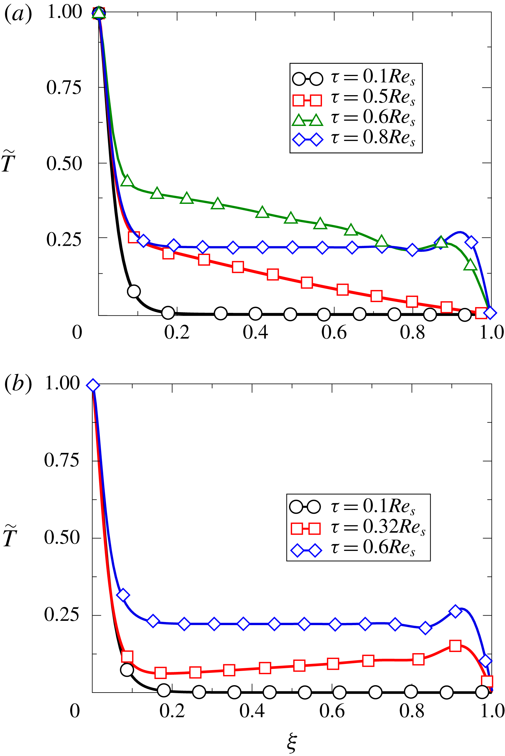
gives rise to a constant source of heat. This can be seen in figure 11(a), where the instantaneous distribution of the temperature at
 $\unicode[STIX]{x1D70F}\simeq 0.5Re_{s}$
exhibits a linear profile due to the heating that a fluid particle undergoes while moving from the stator to the rotor. The transition of the temperature field from stage II to stage III is due to the appearance of a radial convection of temperature, represented by the term
 $2F\tilde{T}_{2}$
, in a dimensionless time of
 $\unicode[STIX]{x1D70F}\sim Re_{s}$
. This radial convection gives rise to the creation of Bödewadt’s boundary layer with its associated dissipation and heat source. The enthalpy created in the stator region gives rise to a step change of temperature from
 $\unicode[STIX]{x1D70F}\simeq 0.5Re_{s}$
to
 $\unicode[STIX]{x1D70F}\simeq 0.6Re_{s}$
, see figure 11(a). Finally the steady state is obtained approximately at
 $\unicode[STIX]{x1D70F}\simeq 0.8Re_{s},$
where the thermal energy created in the stator is transported first to the rotor and then radially in the rotor boundary layer.
If we now consider the case for which at
 $\unicode[STIX]{x1D70F}=0$
,
 $G_{0}=10^{-4}$
, analogously to what happened in the velocity field, the diffusive (stage II) is bypassed. As shown in figure 11(b) at
 $\unicode[STIX]{x1D70F}\simeq 0.32Re_{s}$
, the distribution of temperature along the axial direction is not constant, so when the Bödewadt boundary layer is created, the global balance is established by axial and tangential convection, until it reaches the steady solution, as shown at
 $\unicode[STIX]{x1D70F}\simeq 0.6Re_{s}$
in figure 11(b). In this case, simultaneously with the creation of the stator boundary layer, the heat created in the stator region is transported to the disk; since the heating in the stator increases with time, the slope of the temperature profile at
 $\unicode[STIX]{x1D70F}=0.32Re_{s}$
is negative.
Concerning the transient development of the thermal field, if we define the local Nusselt number,
 $Nu_{l}$
, using the instantaneous bulk temperature of the core region, then
 $$\begin{eqnarray}Nu_{l}=\frac{q_{wall}\,s}{k(T_{R}-T_{core})}=\frac{1}{1-\tilde{T}_{core}(\unicode[STIX]{x1D70F},\tilde{r})}\,Nu.\end{eqnarray}$$
If we assume that
 $Nu_{rotor}$
remains constant along time evolution (see figure 10), since the temperature in the core varies with time (see figure 9), the local Nusselt number previously defined increases with time.
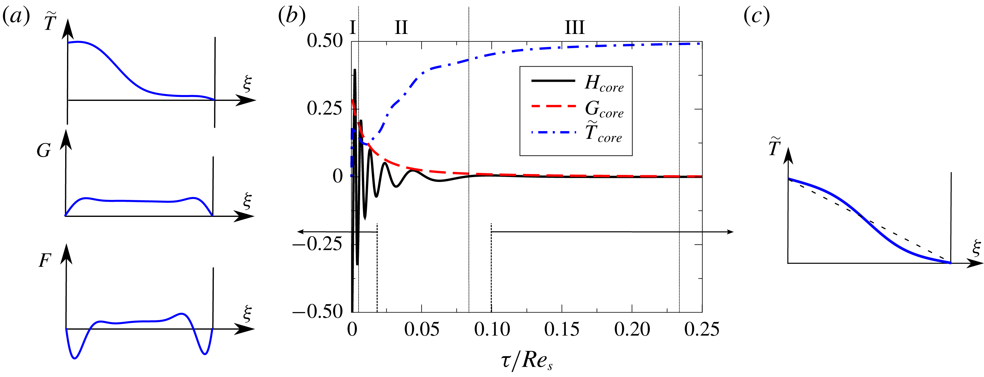
Instantaneous spin-down. The transient evolution of the velocity and temperature in the core region of an infinite cavity between two disks, when initially one disk is rotating and the other is at rest, and the rotor is impulsively stopped, is now studied. The first stage of the process is the very rapid destruction of the von Kármán boundary layer of the rotor and the creation of a new Bödewadt boundary layer (stage I) in dimensionless times of order unity,
 $\unicode[STIX]{x1D70F}_{I}\sim \mathit{O}(1)$
. The azimuthal velocity profile increases from zero at the rotor wall (now at rest) to the core velocity, which is the one corresponding to the steady state before the spin-down.
A sketch of this initial stage is shown in figure 12(a). Once the circumferential velocity in the core of the cavity begins to decrease due to viscous effects (stage II), the Bödewadt boundary layer in the originally stationary disk is adapted to the new conditions outside the boundary layer. The axial velocity, positive in the left disk and negative on the right disk, is instantaneously changed from a negative value to a positive, which means that the convective axial component transports the temperature at the rotor to the core region until the solution reaches steady thermal equilibrium where
 $\widetilde{T}_{core}=0.5$
.
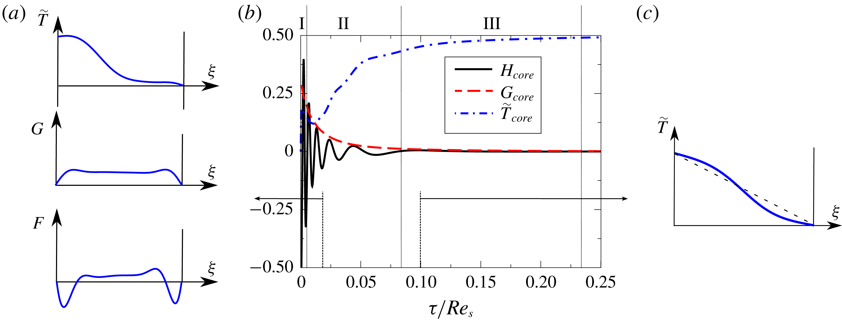
Dimensionless axial, circumferential velocities and temperature at the midpoint of the core region (
 $\unicode[STIX]{x1D709}=0.5$
) as a function of dimensionless time scaled with the diffusive time at
 $Re_{s}=4000$
for a spin-down regime where the rotating disk is suddenly stopped (b). Velocity fields at (a)
 $\unicode[STIX]{x1D70F}=0.02Re_{s}$
(stage II) and (c)
 $\unicode[STIX]{x1D70F}=0.1Re_{s}$
(stage III).
During this stage, the two Bödewadt boundary layers are not in equilibrium since, in general, they are not symmetric due to the fact that the swirling factor of the core,
 $\unicode[STIX]{x1D6FD}$
, is steadily decreasing with time. Both the tangential momentum and the axial mass flow are balanced by means of inertial waves which give rise to steep gradients in all the variables, especially in the axial velocity, as shown in figure 12. The global balance of momentum and mass is continuously updated by axial convection in a time of the order of that needed by the fluid particles to move from the stator to the core,
 $\unicode[STIX]{x1D70F}_{r}\sim Re_{s}^{1/2}$
, giving rise to oscillations in the axial velocity.
The subsequent stage III is of a diffusive nature and its characteristic time is of the order of
 $\unicode[STIX]{x1D70F}_{t}\sim Re_{s}$
. The fluid reaches the actual rest state, although at the end of stage II it can be considered that the fluid velocity is zero. The most noticeable macroscopic effect during this phase in the diffusion of the temperature field, until a linear temperature profiled is attained in the cavity. However, although hardly seen in figure 12,
 $G$
and
 $H$
also are smoothed out by diffusion. The characteristic time of this stage is
 $\unicode[STIX]{x1D70F}_{III}\sim Re_{s}$
, which is very long. This can be seen in figure 12(c).
2.3 Evaluation of unsteady effects
Impulsive start-up is usually considered an instantaneous process in which the disk reaches its final speed. In practice, any ramp-up process occurs in a finite time. We consider here that the rotational speed of the rotor is increased linearly with time, departing from zero and reaching a stationary value. If we name the dimensionless speed-up time
 $\unicode[STIX]{x1D70F}_{s}$
, we can write
 $\unicode[STIX]{x1D6FA}$
as
 $$\begin{eqnarray}\unicode[STIX]{x1D6FA}=\frac{\unicode[STIX]{x1D70F}}{\unicode[STIX]{x1D70F}_{s}}\unicode[STIX]{x1D6FA}_{f}\quad 0\leqslant \unicode[STIX]{x1D70F}\leqslant \unicode[STIX]{x1D70F}_{s}\quad \text{and}\quad \unicode[STIX]{x1D6FA}=\unicode[STIX]{x1D6FA}_{f}\text{ if }\unicode[STIX]{x1D70F}>\unicode[STIX]{x1D70F}_{s}.\end{eqnarray}$$
The wall temperature, both at the rotor and the stator, is assumed to be constant. The change of the rotational velocity of the rotor gives rise to the variation of
 $Re_{s}(\unicode[STIX]{x1D70F})$
and
 $Ec_{r}(\unicode[STIX]{x1D70F})$
with time, reaching their final value,
 $Re_{s,f}$
and
 $Ec_{r,f}$
, at the dimensionless time
 $\unicode[STIX]{x1D70F}_{s}$
.
The objective of this subsection, and of the previous analyses, is to elucidate when the heat transfer at the wall can be computed using a quasi-steady approximation during a disk transient. Fully coupled fluid–solid transient analyses of realistic gas turbine cavities have been computed in the past (Ganine et al. Reference Ganine, Javiya, Hills and Chew2012; Altuna et al. Reference Altuna, Chaquet, Corral, Gisbert and Pastor2013).
To reduce the computational cost the transient behaviour of the solid is computed, but frequently the fluid is considered quasi-stationary. In other words, a series of steady simulations with varying boundary conditions is computed, where the time plays the role of a parameter since time derivatives are neglected in the fluid. The objective of this work is to determine if this quasi-steady hypothesis holds.
One-dimensional analytical model: time evolution scaled with the convective time of dimensionless temperature at the core region (
 $\unicode[STIX]{x1D709}=0.5$
) for different dimensionless speed-up times.
 $Re_{s,f}=4000$
,
 $Pr=0.71$
,
 $Ec_{r,f}=1$
.
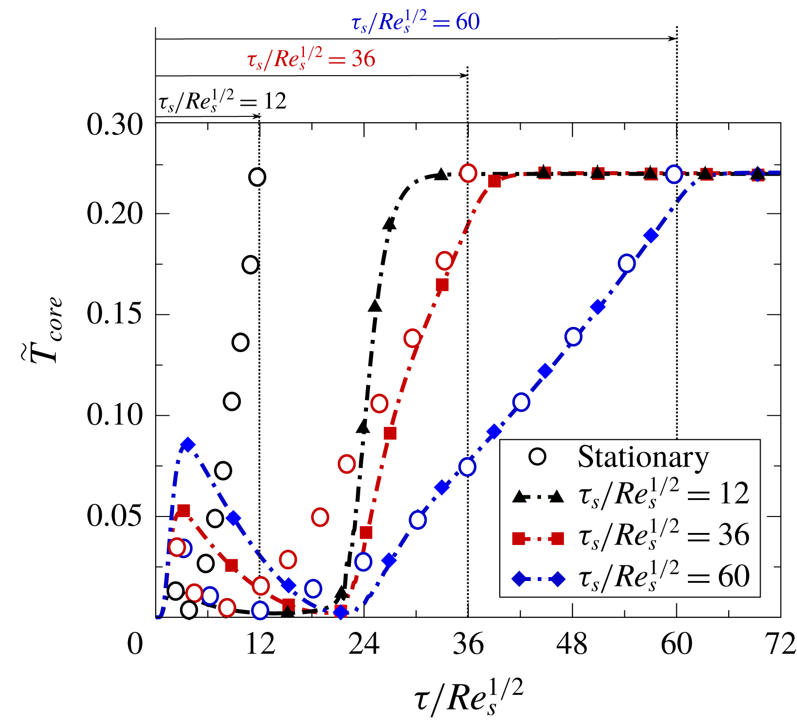
Figure 13 displays the transient evolution of our model rotor–stator cavity for
 $Re_{s,f}=4000$
. The conclusions derived from this relatively low
 $Re_{s}$
can be readily extended to higher, and more realistic,
 $Re_{s}$
, provided that the flow remains laminar. The non-dimensional temperature in the core is represented as a function of the non-dimensional time,
 $\unicode[STIX]{x1D70F}/Re_{s}^{1/2}$
. The reason for this is that the non-dimensional characteristic time of the evolution of an initialised cavity is
 $\unicode[STIX]{x1D70F}_{c}\sim Re_{s}^{1/2}$
.
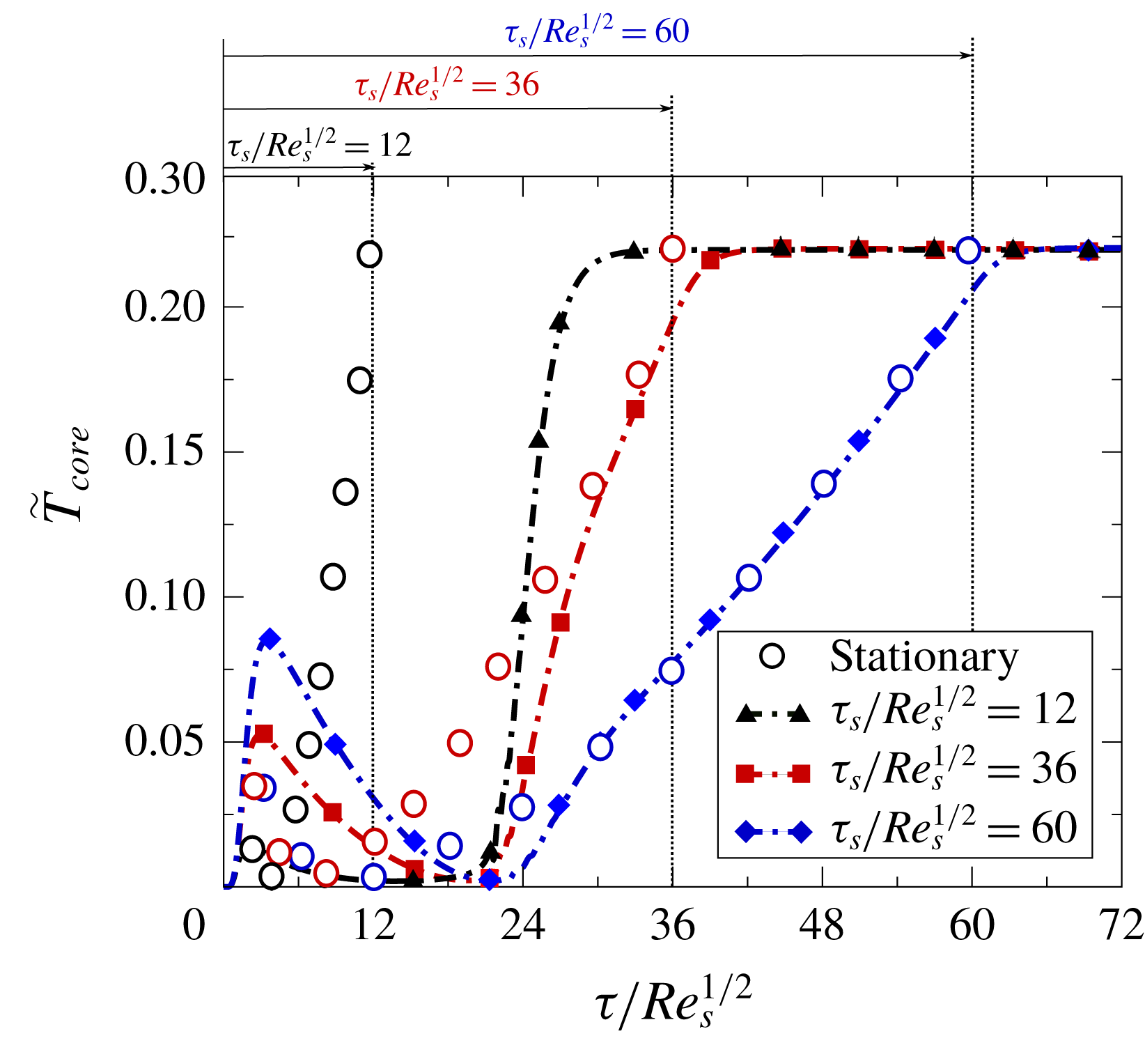
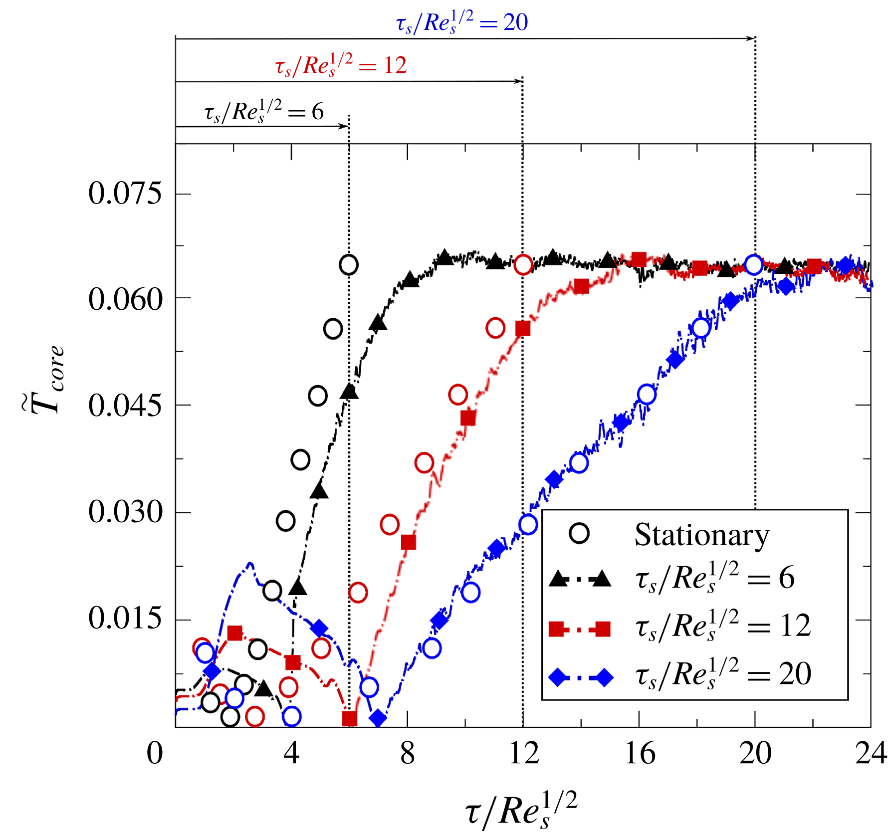
Ramps of different duration have been considered,
 $\unicode[STIX]{x1D70F}_{s}/Re_{s}^{1/2}=12$
, 36 and 60. Lines represent the true transient evolution of the problem, whereas solid symbols correspond to steady solutions for the instantaneous values of
 $Re_{s}(\unicode[STIX]{x1D70F})$
and
 $Ec_{r}(\unicode[STIX]{x1D70F})$
. If the time derivatives were negligible, the solid symbols should superimpose on the different lines. The vertical lines in the same figure mark the end of the ramp. It can be seen that, for very short times, for which
 $Re_{s}(\unicode[STIX]{x1D70F})$
and
 $Ec_{r}(\unicode[STIX]{x1D70F})$
are relatively low, the evolution of the
 $\tilde{T}_{core}$
exhibits a weird behaviour. We do not intend here to describe this complex process involving very thick boundary layers, to avoid missing the whole picture of the problem. For the fastest ramps (
 $\unicode[STIX]{x1D70F}_{s}/Re_{s}^{1/2}=12$
and 36) the quasi-steady solutions have little to do with the true transient solution. For
 $\unicode[STIX]{x1D70F}_{s}/Re_{s}^{1/2}=12$
the temperature in the core is largely over-predicted, whereas for
 $\unicode[STIX]{x1D70F}_{s}/Re_{s}^{1/2}=36$
, the last part of the ramp follows the quasi-steady hypothesis. The slowest ramp (
 $\unicode[STIX]{x1D70F}_{s}/Re_{s}^{1/2}=60$
), however, matches reasonably well with the quasi-steady solution. It is concluded, as expected, that unless
 $\unicode[STIX]{x1D70F}_{s}\gg Re_{s}^{1/2}$
, the quasi-steady hypothesis is not valid. In physical terms, this means that
 $$\begin{eqnarray}t_{ramp}\gg t_{c}=\frac{s}{(\unicode[STIX]{x1D6FA}\unicode[STIX]{x1D708})^{1/2}}=\unicode[STIX]{x1D6FA}^{-1}Re_{s}^{1/2},\end{eqnarray}$$
where
 $t_{ramp}$
is the acceleration time of the ramp. Typically the acceleration time of a large gas turbine is of the order of a few seconds. If we assume that
 $Re_{s}\sim 10^{6}$
and
 $\unicode[STIX]{x1D6FA}\sim 2000~\text{rpm}$
, then
 $t_{c}\simeq 5\text{s}$
. It is therefore concluded that the use of a quasi-steady approach is questionable for this kind of application.
3 Comparison with two-dimensional axisymmetric simulations
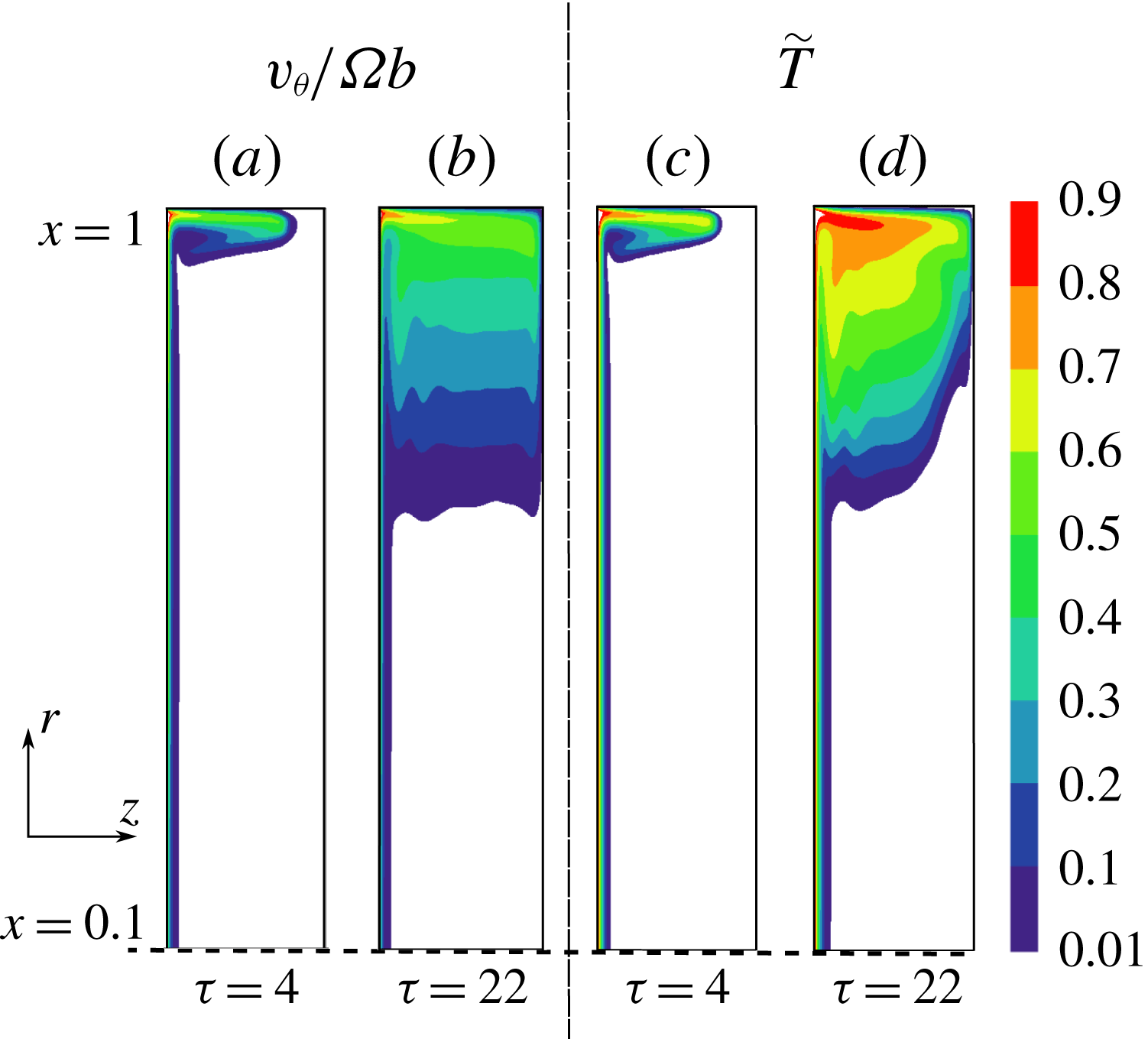
In order to validate the simplified numerical model, several two-dimensional unsteady simulations at different Reynolds numbers were performed. The flow solver, known as
 $Mu^{2}s^{2}T$
(Burgos, Contreras & Corral Reference Burgos, Contreras and Corral2011; Corral, Gisbert & Pueblas Reference Corral, Gisbert and Pueblas2017), is based on a second-order discretisation, both in space and time, of the Navier–Stokes equations. Turbulence models were switched off to force the flow to remain laminar. A confined finite rotor–stator cavity with a non-rotating casing with a wall temperature
 $T_{S}$
, located at the rim of the cavity, is considered. The cavity includes the axis and the outer radius of the cavity is
 $r_{f}=b$
. A
 $450\times 100$
mesh in the
 $(r,z)$
frame proved to be sufficient for the calculation of the rotor–stator cavity with a gap-to-radius ratio of
 $Y=s/b=0.2$
. The Reynolds number based on the radius,
 $Re_{\unicode[STIX]{x1D719}}=Y^{-2}Re_{s}$
, is large (
 $Re_{\unicode[STIX]{x1D719}}\simeq 10^{5}$
) but the flow is assumed to remain laminar (regime II according to Daily & Nece Reference Daily and Nece1960), and hence the stator and rotor boundary layers are separated by a core inviscid region.
The presence of a cylindrical casing at a finite radial distance has an important effect on the transient and steady behaviour of the cavity. It can also alter the global stability of the flow, causing major disruptions of the layer, possibly unrelated to the stability of the Bödewadt boundary layer (Lopez & Weidman Reference Lopez and Weidman1996). Lopez et al. (Reference Lopez, Hart, Marques, Kittelman and Shen2002) have reported that a confined rotor–stator cavity with
 $Y=0.2$
and a rotating shroud is linearly stable with respect to axisymmetric perturbations, at least up to
 $Re_{\unicode[STIX]{x1D719}}\simeq 10^{5}$
. The results presented here are obtained using an axisymmetric formulation of the problem so that the appearance of three-dimensional spiral waves is avoided by construction.
3.1 Steady solution
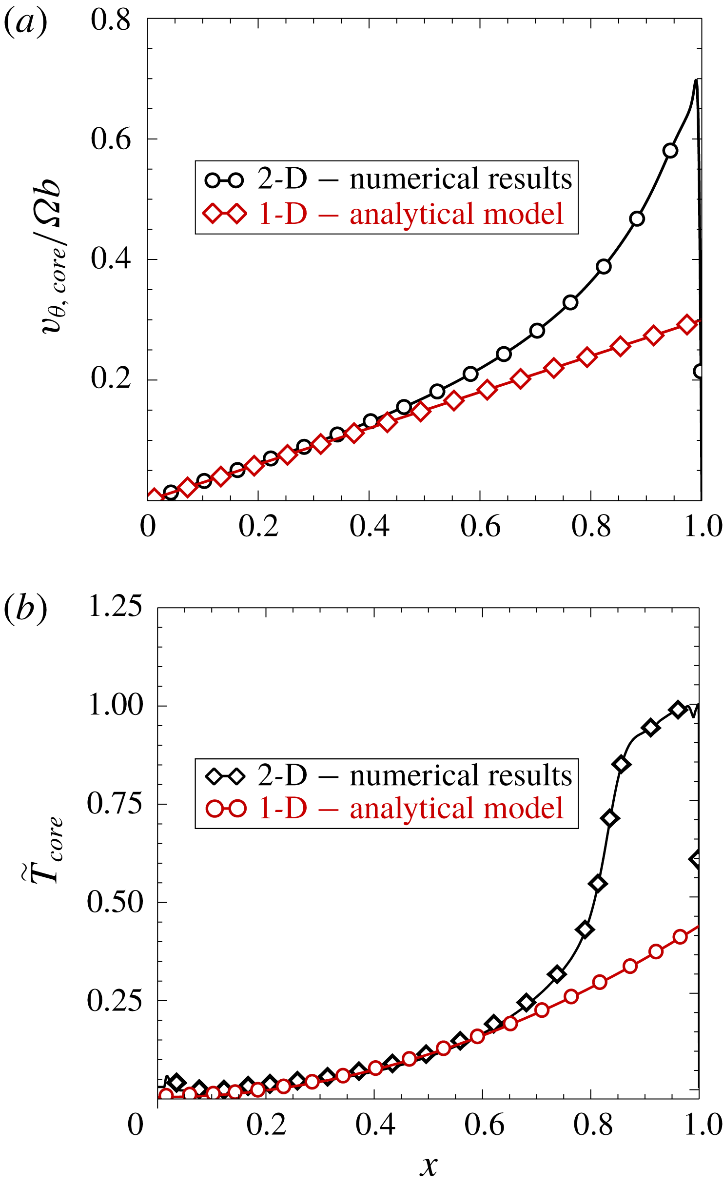
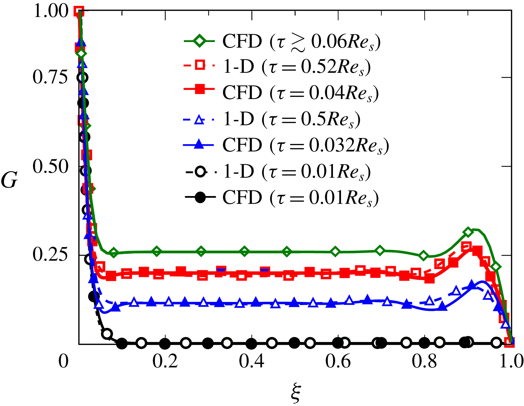
The influence of a stationary outer shroud on the steady state of the core region of a square cavity at high Reynolds numbers is displayed in figure 14. In the inner region of the cavity, and up to
 $x\simeq 0.5$
, both the dimensionless circumferential velocity (figure 14
a) and temperature (figure 14
b) agree very well with the self-similar solution, where the dimensionless radial distance is defined as
 $x=r/b$
. This fact had been previously reported for the velocity field (Dijkstra & van Heijst Reference Dijkstra and van Heijst1983; Brady & Durlofsky Reference Brady and Durlofsky1987), but here it is shown that the same is true as well for the thermal field. The circumferential velocity in the inner region varies linearly with the radius, equation (3.1), and the swirl factor at the core is
 $\unicode[STIX]{x1D6FD}\backsimeq 0.31$
(Itoh et al.
Reference Itoh, Yamada, Imao and Gonda1992), which corresponds to the value expected for a high Reynolds laminar flow, as has been previously mentioned:
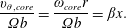 $$\begin{eqnarray}\frac{v_{\unicode[STIX]{x1D703},core}}{\unicode[STIX]{x1D6FA}b}=\frac{\unicode[STIX]{x1D714}_{core}r}{\unicode[STIX]{x1D6FA}b}=\unicode[STIX]{x1D6FD}x.\end{eqnarray}$$
Concerning the temperature distribution along the radius in the core (figure 14
b), the self-similar and CFD solutions match very well up to
 $x\simeq 0.6$
, but for higher values of the radius, the effect of the outer stationary casing spoils the self-similar solution, as could be expected. Taking into account that
 $\tilde{r}=x/Y$
, we can express the temperature in the core as a function of the
 $Ec$
number, equation (2.36), as
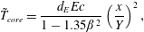 $$\begin{eqnarray}\tilde{T}_{core}=\frac{d_{E}Ec}{1-1.35\unicode[STIX]{x1D6FD}^{2}}\left(\frac{x}{Y}\right)^{2},\end{eqnarray}$$
which corresponds to the quadratic trend of temperature that is seen in figure 14(b). If
 $Ec_{b}\sim \mathit{O}(1)$
, as is the case here (
 $Ec_{b}\simeq 2$
), then
 $\tilde{T}_{core}\sim \mathit{O}(1)$
. For small values of the radius
 $Ec_{r}\ll 1$
, the fluid cannot be heated by viscous dissipation (as is also shown in figure 14
b).
Influence of a stationary outer shroud on the steady laminar flow (
 $Re_{s}=4000$
,
 $Re_{\unicode[STIX]{x1D719}}\simeq 10^{5}$
) at the midpoint of the core region (
 $\unicode[STIX]{x1D709}=0.5$
) of a square cavity with a gap ratio
 $Y=0.2$
. (a) Dimensionless azimuthal velocity. (b) Dimensionless temperature.
 $Pr=0.71$
,
 $Ec=8\times 10^{-2}$
.
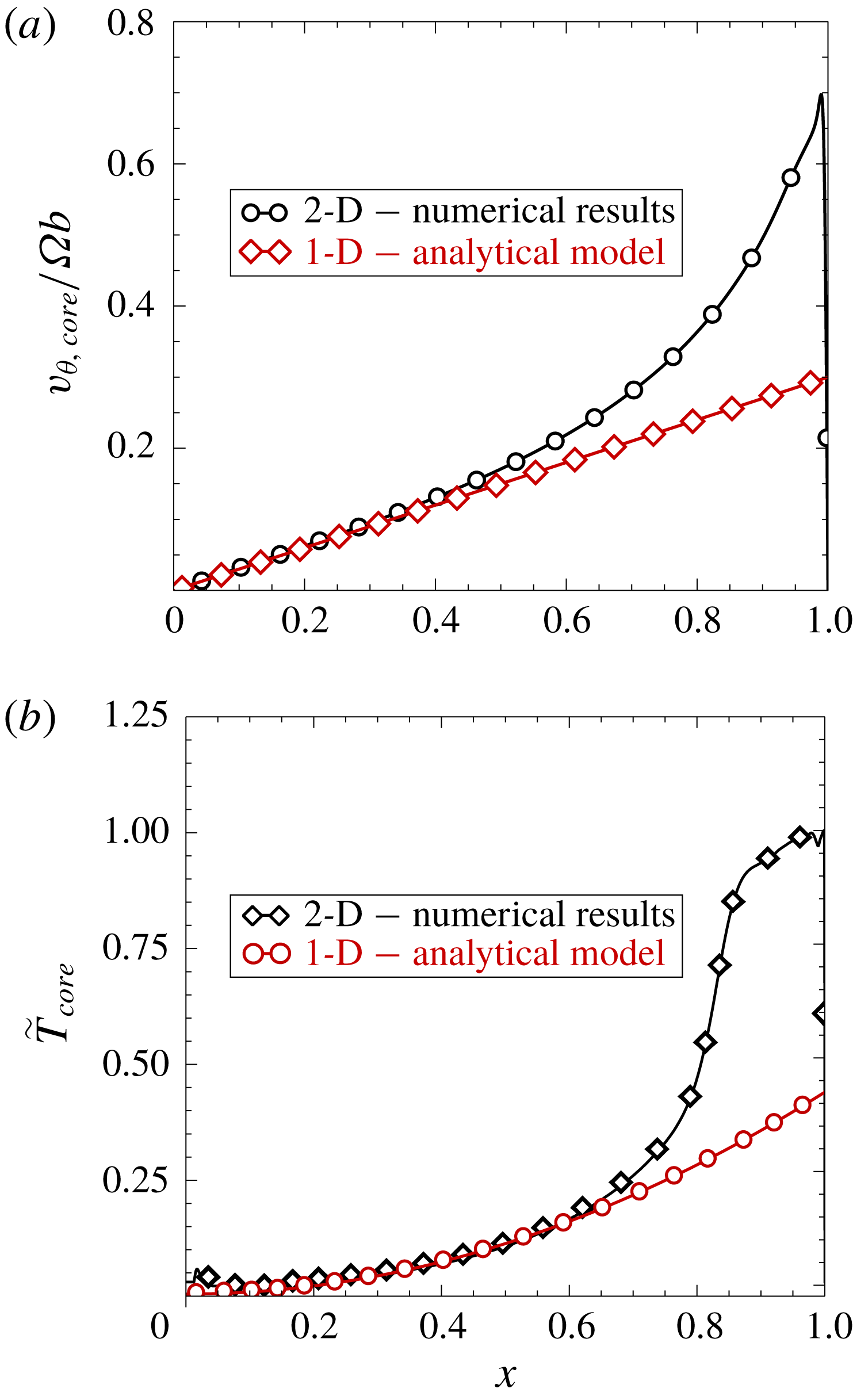
3.2 Unsteady solutions
This subsection aims to assess the impact of a stationary outer shroud on the transient behaviour of an enclosed cavity using axisymmetric laminar analyses. As discussed by van Eeten et al. (Reference van Eeten, van der Schaaf, van Heijst and Schouten2013), the presence of the outer casing has a relevant impact on both the steady and the transient solutions of the problem. This casing imposes either a zero or 1 swirl factor, depending on whether or not it is rotating, and spoils the self-similar solution in the vicinity of the outer casing, which has a constant swirl factor along the radius. The transient start-up process of the cavity has three distinct phases, the second of them differing from that identified in the self-similar one-dimensional analysis. Once the rotor is impulsively set into motion, in a very short time, of the order of the diffusive time (
 $\unicode[STIX]{x1D70F}_{I}\sim \mathit{O}(1)$
), the von Kármán boundary layer is created in the rotor, and the flow inside a very thin boundary moves radially outwards, until it impinges on the outer casing. The flow is then deflected horizontally, transporting the tangential momentum and enthalpy which was previously created in the disk boundary layer to the core (see figure 15
a,c). The inward flow, of the already existing Stewartson-type flow, transports the angular momentum and enthalpy located in the outer core region of the cavity. Since the characteristic radial velocity in the core is
 $v_{rc}\sim \unicode[STIX]{x1D6FA}rRe_{s}^{-1/2}$
, the characteristic time needed for a particle to move from the outer radius of the disk,
 $b$
, to a radius
 $r$
is
 $\unicode[STIX]{x1D70F}_{II}\sim Re_{s}^{1/2}\ln (b/r)$
, which is large since the radial velocity is very small. This phase of the transient development does not exist in the one-dimensional model, since in this approach the swirl factor along the radius is deemed to be constant during the transient period and the velocity field is assumed to vary linearly with the radius. This phenomenon triggers the convective transport term of angular momentum (figure 15
b,d). During this phase, and in the upper region of the cavity, the inward flow is in the core, not in the stator boundary layer, which at this stage has not yet been created. Finally, when at a certain radius the circumferential velocity reaches a finite value, Batchelor flow is created, and there is a third phase in which the fluid is transported from the stator to the rotor. This time is also long and this phase, in the core of the cavity, is similar to that described in the one-dimensional model (
 $\unicode[STIX]{x1D70F}_{III}\sim Re_{s}^{1/2}$
), and is associated with the convection of fluid from the stator to the rotor. It is concluded that, in a laminar enclosed cavity, the characteristic time of the transient is
 $\unicode[STIX]{x1D70F}\sim Re_{s}^{1/2}$
, and the long diffusive phase identified in the one-dimensional model is always bypassed.
Dimensionless azimuthal velocity,
 $v_{\unicode[STIX]{x1D703}}/\unicode[STIX]{x1D6FA}b$
, and temperature,
 $\widetilde{T}$
, contour plots on a finite laminar rotor–stator cavity at two different dimensionless times: (a,c)
 $\unicode[STIX]{x1D70F}=4$
, (b,d)
 $\unicode[STIX]{x1D70F}=22$
.
 $Re_{s}=4000$
,
 $Pr=0.71$
,
 $Ec=8\times 10^{-2}$
,
 $Y=0.2$
.
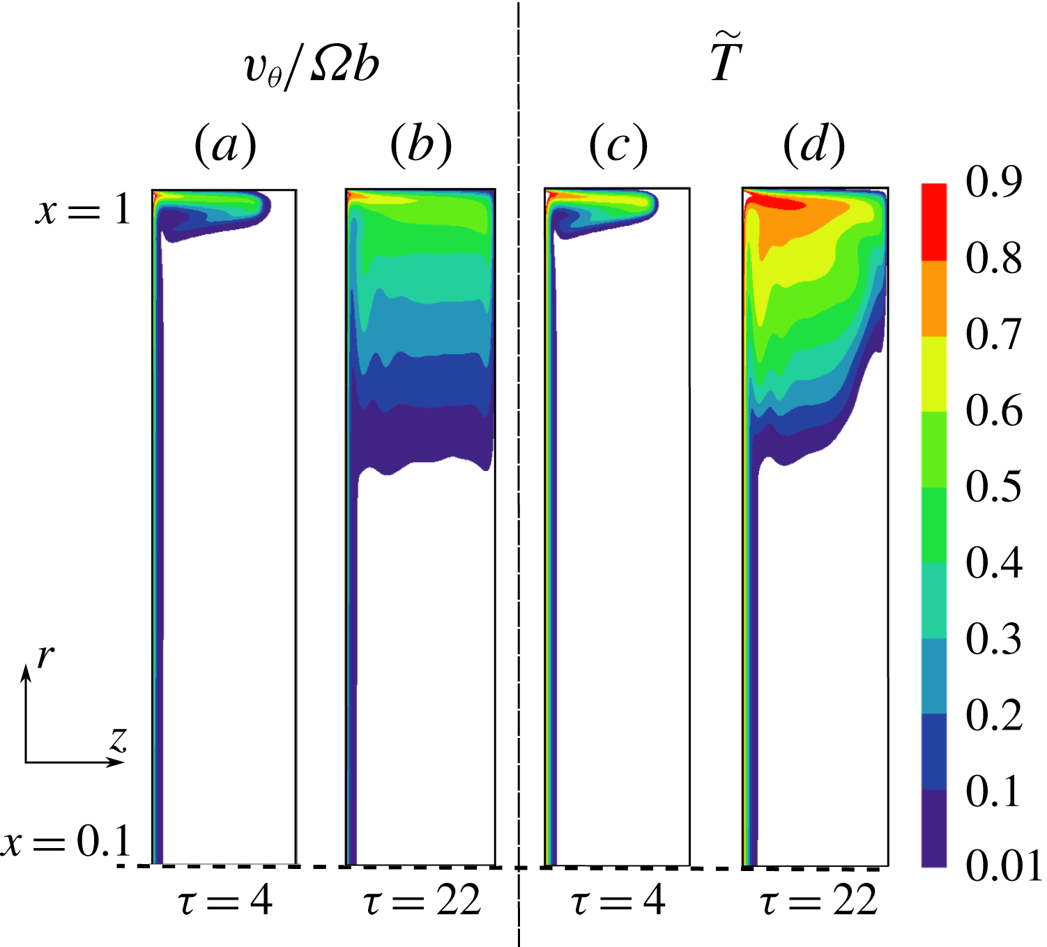
The practical relevance of the transient analysis of the flow in a rotor–stator cavity has mainly to do with its impact in the heat exchange between the cavity and the disks. Let us consider the energy transfer evolution during the impulsive start of one of the two coaxial disks enclosing a fluid cavity. The energy equation of the disk in integral form is
 $$\begin{eqnarray}\bar{\unicode[STIX]{x1D70C}}V\frac{\text{d}E}{\text{d}t}=\underbrace{\int _{r}k\unicode[STIX]{x1D735}T\cdot \text{d}A}_{Q_{rotor}}+\underbrace{\int _{s}k\unicode[STIX]{x1D735}T\cdot \text{d}A}_{Q_{stator}}+\underbrace{\int _{c}k\unicode[STIX]{x1D735}T\cdot \text{d}A}_{Q_{casing}}+\underbrace{\int _{r}(\unicode[STIX]{x1D70F}^{\prime }\cdot v)\cdot \text{d}A}_{Q_{windage}},\end{eqnarray}$$
where
 $\bar{\unicode[STIX]{x1D70C}}$
is the mean density of the cavity,
 $E$
is the total energy,
 $V$
its volume,
 $Q_{rotor}$
,
 $Q_{stator}$
,
 $Q_{casing}$
the energy transferred by conduction between the fluid and the rotor, stator and casing respectively and
 $Q_{windage}$
is the energy transferred from the disk to the fluid by viscous friction. In order to numerically show the characteristic time to reach the steady state, we non-dimensionalise the energy in the following way:
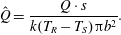 $$\begin{eqnarray}\hat{Q}=\frac{Q\cdot s}{k(T_{R}-T_{S})\unicode[STIX]{x03C0}b^{2}}.\end{eqnarray}$$
Figure 16 displays the time evolution of the different terms of the energy equation (3.3) of the cavity in integral form. The dimensionless time needed to reach the steady state in the cavity is approximately
 $\unicode[STIX]{x1D70F}_{t}\simeq 5.2Re_{s}^{1/2}$
. The heat flux at the rotor and the mechanical energy transferred from it to the fluid are nearly constant after a very short time. The same is true for the outer casing, which quickly reaches its final state once the hot fluid coming from the rotor boundary wets the shroud. The heat flux at the stator departs from zero and increases when the core of the cavity is heated with hot fluid coming from the outer shroud due to the inward radial convection at the core. This process takes place with the simultaneous creation of the Bödewadt boundary layer in the stator. It is concluded, as can be seen in figure 16, that the characteristic time of the transient of this two-dimensional model cavity is
 $\unicode[STIX]{x1D70F}_{c}\propto Re_{s}^{1/2}$
, exactly as in the one-dimensional model, although for different physical reasons.
Transient evolution scaled with the convective time of the components of the energy balance of a rotor–stator cavity with gap ratio
 $Y=0.2$
, represented by Nusselt number based on the outer radius. Case of
 $Re_{s}=4000$
,
 $Pr=0.71$
,
 $Ec=8\times 10^{-2}$
.
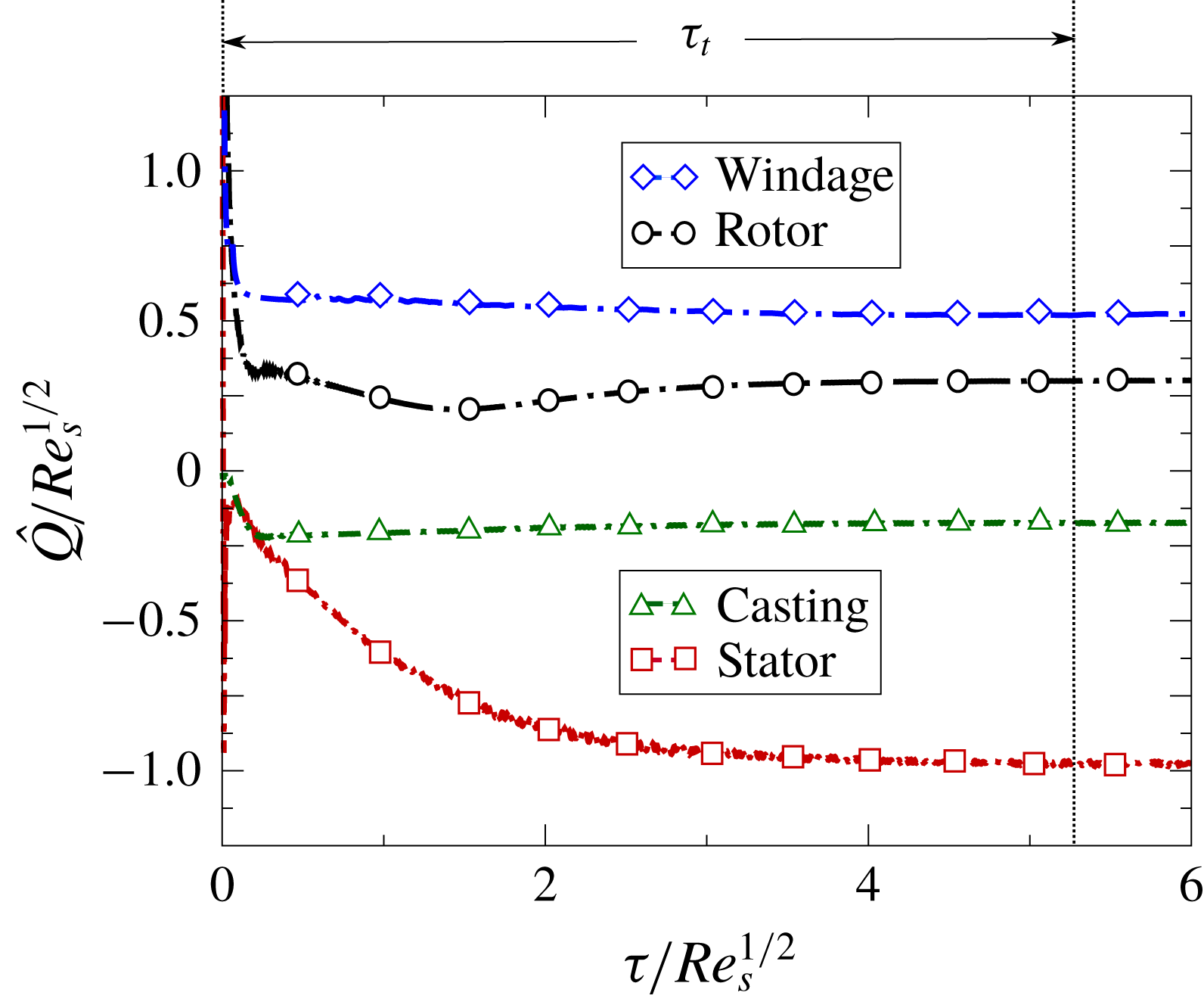
Comparison of the non-dimensional circumferential velocity profiles obtained from two-dimensional numerical simulations and from the simplified similarity analysis at different time instants at the same dimensionless radius (
 $x=0.45$
).
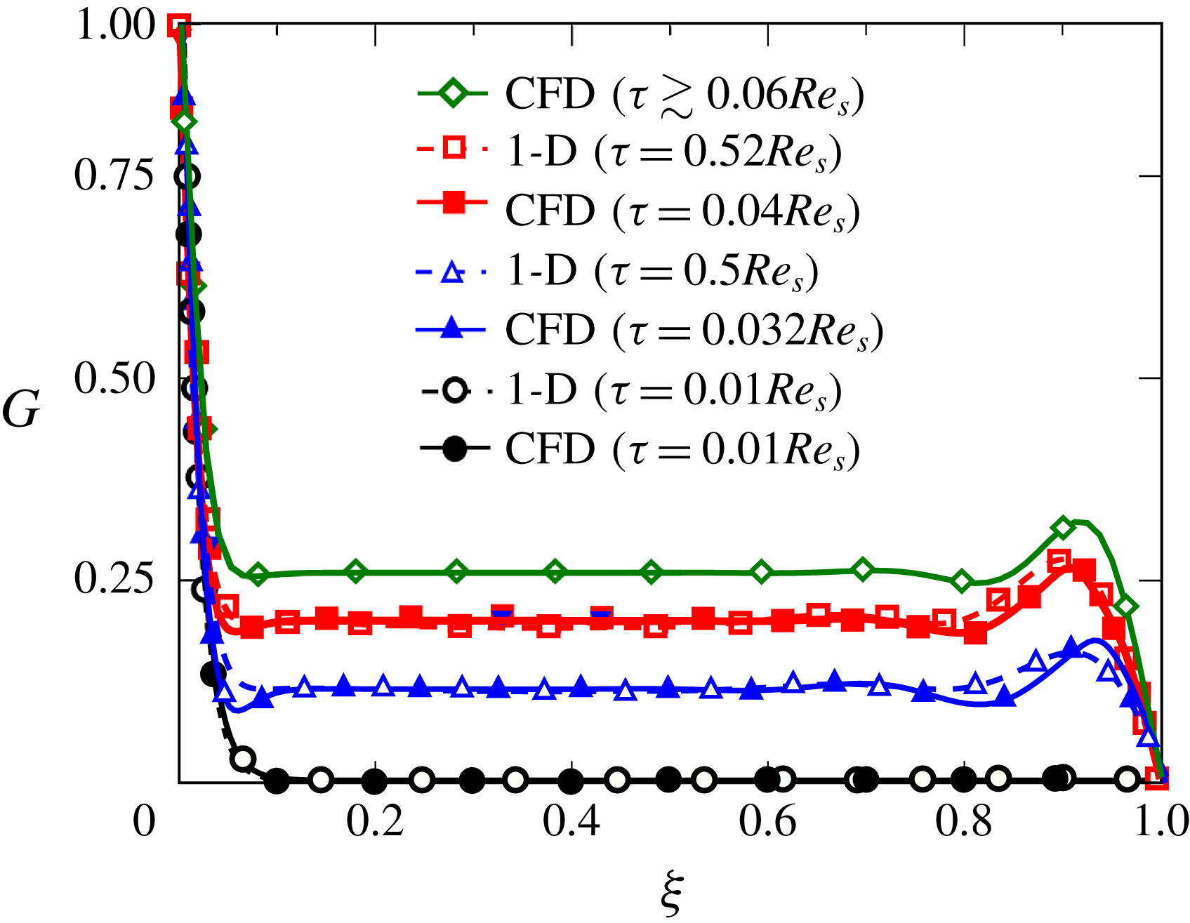
3.2.1 CFD comparison with one-dimensional analytical model
It can finally be questioned whether the flow obeys the similarity analysis during the spin-up or spin-down transients. The similarity solution imposes a strong constraint on the radial variation of the velocity (
 $v_{r}\sim \unicode[STIX]{x1D6FA}r$
and
 $v_{\unicode[STIX]{x1D703}}\sim \unicode[STIX]{x1D6FA}r$
) which cannot capture the radial waves identified by Lopez et al. (Reference Lopez, Marques, Rubio and Avila2009) in the Bödewadt boundary layer during the spin-down of a square cavity. However, since these perturbations die out in a very short time (
 $\unicode[STIX]{x1D70F}\sim \mathit{O}(1)$
), we assume that this process hardly affects the overall transient of the cavity whose characteristic time is much longer (
 $\unicode[STIX]{x1D70F}\sim Re_{s}^{1/2}$
).
In order to assess the similarity hypothesis, figure 17 compares the dimensionless circumferential velocity profiles obtained by the one-dimensional (1-D) similarity analysis and 2-D numerical simulations during the instantaneous spin-up of a square cavity at different time instants for the same radius (
 $x=r/b=0.45$
). The time instants of the 1-D and 2-D solutions are different because the physics of the transient phase of the shrouded cavity is different. Moreover, we have constructed the figure with the profiles obtained from the similarity analysis when the fluid is initially at rest (
 $G_{0}=0$
). In order to ease the comparison with the results obtained in the previous section for the 1-D self-similar analysis, we express the dimensionless time scaled with
 $Re_{s}$
, although we stress that the time development of stage II in an enclosed cavity is dominated by convective transport of angular momentum from larger to shorter radii, and that the characteristic time of this process is
 $\unicode[STIX]{x1D70F}\sim Re_{s}^{1/2}$
. It can be noticed that at
 $x=0.45$
, the velocity profiles of the 2-D analysis resemble those obtained in the 1-D analysis and that the transient can be seen as a sequence of Stewartson (
 $\unicode[STIX]{x1D70F}=0.01Re_{s}$
) and Batchelor (
 $\unicode[STIX]{x1D70F}\geqslant 0.032Re_{s}$
) type solutions. The core region is present from the very early stages of the process and the swirl factor in the core steadily increases from zero to its final stationary value. The actual times of the snapshot are however quite different, as has already been mentioned, because the start-up processes have a completely different nature.
Figure 18 displays the speed-up process of the same enclosed rotor–stator cavity from rest to a final Reynolds number based on the gap
 $Re_{s,f}=4000$
, for different acceleration times of the disk. The flow remains laminar along the whole process since the final Reynolds number based on the radius is
 $Re_{\unicode[STIX]{x1D719},f}\simeq 10^{5}$
. The counterpart for the 1-D model is the figure 13. The qualitative behaviour for the slowest ramps of the 1-D model (figure 13) and the 2-D model (figure 18), match reasonably well with the quasi-steady solution. The slowest non-dimensional acceleration times are
 $\unicode[STIX]{x1D70F}_{s}/Re_{s}^{1/2}=60$
for the 1-D model, and 20 for the CFD model, reflecting the fact that the response of the square cavity is faster than that of ideal infinite cavity. As previously mentioned, the non-dimensional characteristic time of evolution is of order
 $\unicode[STIX]{x1D70F}_{c}\sim Re_{s}^{1/2}$
for both cases, and unless
 $\unicode[STIX]{x1D70F}_{s}\gg Re_{s}^{1/2}$
, the quasi-steady hypothesis is not valid for a realistic enclosed cavity or for an infinite cavity. This condition, in general, is not fulfilled for transients in gas turbine representative cases.
Time evolution scaled with the convective time of the dimensionless temperature at the core region (
 $\unicode[STIX]{x1D709}=0.5$
) of a two-dimensional rotor–stator closed cavity of aspect ratio
 $Y=0.2$
at a dimensionless radius
 $x=0.4$
for different dimensionless speed-up times.
 $Re_{s,f}=4000$
,
 $Pr=0.71$
,
 $Ec_{r,f}=(x/Y)^{2}\,Ec_{f}=0.32$
.
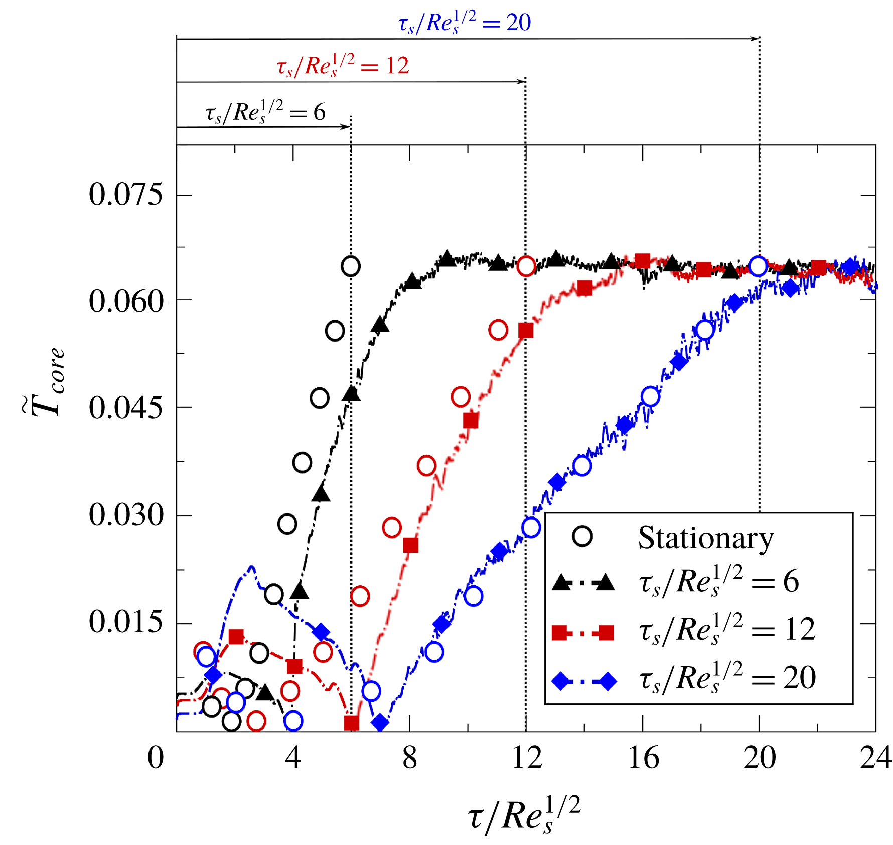
4 Conclusions
The flow field and heat transfer behaviour of a model rotor–stator cavity using the von Kármán self-similar analysis has been revisited. The resulting system of nonlinear time-dependent ODEs has been solved numerically using a second-order method, both in space and time. Numerical results have been obtained for Reynolds numbers ranging between 600 and 30 000 to derive different trends for high Reynolds numbers.
Fundamental concepts and practical conclusions of the flow patterns and heat transfer mechanisms have been drawn. The fluid is considered as incompressible with constant properties, and therefore the flow pattern can be discussed independently of the temperature field if buoyancy effects are neglected. It is concluded that the disk can only heat a very thin region, of the order of
 $\unicode[STIX]{x1D6FF}/s\sim Re_{s}^{-1/2}$
, close to the rotor. This is due to the fact that the axial convection from the stator to the rotor shields the core from the rotor and prevents its heating. The component of the temperature which changes quadratically with the radius,
 $\tilde{T}_{2}$
, which is of order
 $\tilde{T}_{2}\sim Pr\,Ec$
, is then the single mechanism changing the temperature of the core region by axial convection from the Bödewadt boundary layer to the rotating disk. It can be concluded that the temperature increase at the core region (
 $\tilde{T}_{core}\sim Ec_{r}$
) is created by a heat source in the immediate vicinity of the stator disk, due to viscous dissipation. The integral angular momentum and energy balance of the cavity have been investigated to fully understand the balance between the stator and the rotor and to estimate the stationary solution. Non-dimensional heat flux at the rotor is only a function of the Reynolds number based on the gap, and the Eckert number based on the radius
 $Ec_{r}$
, which accounts for the effect of viscous dissipation. The working fluid has been assumed to be air, and hence the dependence with the Prandtl number has not been pursued in this work.
Finally the time-dependent solution predicted by the self-similar analysis has been compared against 2-D axisymmetric laminar simulations, accounting for the effect of the outer shroud of the cavity. It is concluded that the one- and two-dimensional models describe qualitatively the same physics up to 50 % of the radius of the cavity, whereas the outer part of the cavity is heavily influenced by the presence of the casing. The relevance of the transient analysis of the flow in an infinite rotor–stator cavity and its associated characteristic times have been assessed. Viscous and thermal diffusion gives rise in an infinite cavity to very long transients (
 $\unicode[STIX]{x1D70F}_{II}\sim Re_{s}$
) when the cavity is initially at rest, then a third and shorter phase (
 $\unicode[STIX]{x1D70F}_{III}\sim Re_{s}^{1/2}$
) dominated by the axial convection takes place. The long diffusion phase is bypassed when the flow is initialised with a small perturbation. The same is true in real enclosed cavities, where the presence of an outer shroud at a finite radial distance changes the dynamics of the process. In this case, there is an inward radial convection departing from the outer shroud. It has been shown that the characteristic time of this phase is also
 $\unicode[STIX]{x1D70F}_{c}\sim Re_{s}^{1/2}$
, and it is associated with the radial convection. It is concluded that in realistic applications the diffusive phase of the process can rarely be seen.
For large Reynolds numbers, only when the acceleration time of the disk is much greater than
 $s/(\unicode[STIX]{x1D6FA}\unicode[STIX]{x1D708})^{1/2}$
does the hypothesis that the flow is quasi-stationary hold. This hypothesis is quite often not fulfilled. It is concluded that the flow unsteadiness cannot be disregarded in the simulations and that the validity of quasi-steady methodologies used in gas turbine representative problems is either doubtful or not appropriate.
The flow in finite rotor–stator cavities very rapidly develops instabilities leading to turbulence. It should be recalled that the conclusions derived in this work are valid as long as the flow remains stable and laminar. The characteristic times for a turbulent flow are different. However, here, the purpose was not to undertake an exhaustive investigation of all the effects but to create a building block of knowledge aimed at increasing the understanding of cavity flows in more complex situations under the assumptions made on this manuscript. The effect of transition and turbulent mixing certainly have to be taken into account in real applications, and it is speculated that the quasi-steady assumption may also fail in this case but under different conditions.
Acknowledgements
R.C. and D.R. wish to thank Industria de Turbopropulsores S.A.U. for allowing the publication of this paper and for its support during the project. This work was carried out under ITP contract no. DTP/ITP/16/001, UPM Project no. P1614120148. R.C. also wants to thank Professor Amable Liñan for lecturing on similarity analysis and perturbation methods in several undergraduate and graduate courses at the School of Aeronautics of the UPM.