1. INTRODUCTION
Since its introduction in 1960, the Kalman filter has been widely used to estimate the parameters of kinematic systems (Gelb et al., Reference Gelb, Kasper, Nash, Price and Sutherland2001). The classical Kalman filter is, by nature, a form of least-squares estimation. Thus it is sensitive to observation outliers and/or abrupt changes, which may make the estimates too optimistic, and even cause the algorithm to diverge. To deal with this problem, various robust adaptive methods have been presented. The quality control Detection, Identification, and Adaptation theory has been coupled with a Kalman filter to detect model errors (Teunissen, Reference Teunissen1990). Additive approaches for detecting abrupt changes have been developed that use likelihood ratios, multiple models, and algebraic tests (Gustafsson, Reference Gustafsson2000). Adaptive factors are typically used to cope with kinematic model discrepancies. Various adaptive factor calculation schemes have been compared, and a new approach that employs an exponential model to construct the adaptive factor was introduced. Two optimal adaptive factors, based on the estimated covariance matrix of the innovation vector and that of the predicted filtering state vector, were further proposed (Yang and Gao, Reference Yang and Gao2005; Reference Yang and Gao2006). Another approach to accommodate the poor modelling of abrupt kinematic changes is that of a fading memory, whereby the impact of abnormal movement becomes progressively lower with time. An adaptive estimation approach for multiple fading memory factors to discriminate different state vector elements was developed alongside an accompanying statistical test procedure (Jazwinski, Reference Jazwinski1970; Geng and Wang, Reference Geng and Wang2008). Generally, these methods can be divided into two categories: one for functional models, and a second for stochastic models. To prevent the computational load becoming onerous, most research has focused on the second group.
Considerable efforts have been made to deal with both observation outliers and abrupt kinematic changes in the filtering process (Yang et al., Reference Yang, He and Xu2001; Gao et al., Reference Gao, Zhong and Li2011; Hajiyev and Soken, Reference Hajiyev and Soken2013). However, when dealing with outliers, the least-squares or predicted residuals are employed, whereas with abrupt changes in carrier movement we usually assume that all state elements can be directly obtained with a single-epoch observation. Li et al. (Reference Li, Gong, Liu, Chen and Duan2013) introduced a method to adjust the dynamic process noise Variance–Covariance (VCV) matrix by taking the divergence between the VCV matrices of the innovation vector derived from the filter state update procedure and that of the innovation vector correlation. In addition, Koch and Yang (Reference Koch and Yang1998) developed a robust Kalman filter for rank-deficient observation models based on a generalised inverse and robust M-estimate. This is unreasonable if factors from only a part of the state elements are applied to the whole state vector. To overcome this shortcoming, a robust filtering approach that classifies adaptive factors by differencing was introduced by Cui and Yang (Reference Cui and Yang2006).
Robust adaptive Kalman filters usually deal with observation outliers by robust estimation based on least-squares residuals, innovation, or the residuals after the measurement update step. Abrupt changes are handled by adaptive factors that use discrepancies in the innovation or state vector. The robust estimation and adaptive factors operate in a similar manner, in the sense that they are always used to produce an equivalent weight matrix to accommodate the impact of outliers and abrupt changes. As long as they are nonzero, the off-diagonal elements of the VCV matrices will change when multiplied by the robust or adaptive factors. Abrupt changes are not treated properly from the perspective of physical significance. In fact, abrupt changes in a moving state, such as accelerating, decelerating or swerving, are motivated by force. Thus an abrupt acceleration change could be considered as system noise, and then coupled to the position, velocity, and acceleration via the coupling matrix. If an abrupt change occurs, the acceleration will manifest itself in the position components, which can be estimated using a robust technique and data obtained from more than four in-view Global Positioning System (GPS) satellites. Thus, additional kinematic noise is adopted to accommodate abrupt changes, and a robust estimation technique is applied to the observations.
The remainder of this paper is arranged as follows. First, robust adaptive Kalman filtering, in which adaptive factors are applied to readjust a stochastic model, is introduced. Second, a new robust adaptive method for tuning the kinematic and measurement noise VCV matrices is developed. Finally, the efficiency of the proposed algorithm is demonstrated using a relative kinematic positioning case involving a GPS receiver mounted on a plane.
2. TRADITIONAL ROBUST ADAPTIVE KALMAN FILTERING
Let the linear kinematic and observation models of Kalman filtering be
 $${\bi X}_k = {\bi \Phi} _{k,k - 1}{\bi X}_{k - 1} + {\bi \Gamma} _k{\bi e}_k$$
 $${\bi y}_k = {\bi H}_k{\bi X}_k + {\bi v}_k$$
where
 ${\bi X}$
denotes the filtering state,
 ${\bi \Phi} $
is the transition matrix,
 ${\bi H}$
is the observation design matrix,
 ${\bi \Gamma} $
is the kinematic noise coupling matrix,
 ${\bi y}$
is the observation vector and the subscript k indicates the discrete time or epoch. In addition, the stochastic models of kinematic and observation noise are set to be zero-mean white Gaussian and mutually uncorrelated:
 $$E\left( {{\bi e}_k} \right) = {\bi 0}$$
 $$E\left( {{\bi e}_k \cdot {\bi e}_j^T} \right) = \left\{ {\matrix{ {{\bi Q}_k{\rm} \quad j = k} \cr {{\bi 0}{\rm} \quad \ \ j \ne k} \cr}} \right.$$
 $$E\left( {{\bi v}_k} \right) = {\bi 0}$$
 $$E\left( {{\bi v}_k \cdot {\bi v}_j^T} \right) = \left\{ {\matrix{ {{\bi R}_k{\rm} \quad j = k} \cr {{\bi 0}{\rm} \quad \ \ j \ne k} \cr}} \right.$$
 $$E\left( {{\bi e}_k \cdot {\bi v}_j^T} \right) = {\bi 0}\,{\rm \,for \,\,all}\,\,j,k$$
where () denotes the mathematical expectation and D() is the VCV matrix.
A robust adaptive Kalman filtering method for controlling outliers in the observations and updated parameters can be written as (Yang and Gao, Reference Yang and Gao2006):
 $${\bi X}_k^ - = {\bi \Phi} _{k,k - 1}{\bi X}_{k - 1}^ + $$
 $${\bi \Sigma} _k^ - = {\bi \Phi} _{k,k - 1}{\bi \Sigma} _{k - 1}^ + {\bi \Phi} _{k,k - 1}^T + {\bi \Gamma} _{k - 1}{\bi Q}_{k - 1}{\bi \Gamma} _{k - 1}^T $$
 $${\bi X}_k^ + = {\bi X}_k^ - + { \tilde {\bi K}}_k\left( {{\bi y}_k - {\bi H}_k{\bi X}_k^ -} \right)$$
 $${\bi \Sigma} _k^ + = \displaystyle{{\left( {{\bi I} - {\tilde{\bi K}}_k{\bi H}_k} \right){\bi \Sigma} _k^ -} \over {\alpha _k}}$$
where the Kalman gain matrix is
 $${\tilde{\bi K}}_k = \displaystyle{1 \over {\alpha _k}}{\bi \Sigma} _k^ - {\bi H}_k^T \left( {\displaystyle{1 \over {\alpha _k}}{\bi H}_k{\bi \Sigma} _k^ - {\bi H}_k^T + {\bar {\bi R}}_k} \right)^{ - 1}$$
with
 ${\bar {\bi R}}_k$
being the equivalent VCV matrix of the observations, and α
k
(0 < α
k
≤ 1) operating as an adaptive factor (Yang and Gao, Reference Yang and Gao2005). The superscripts T, −1, −, and + denote the matrix transpose, inversion operator, time-update step, and measurement update step of the Kalman filtering routine, respectively.
The detection of observation outliers is usually based on the assumption that the predicted state vector and the stochastic models are correct, and vice versa. This will depress the efficiency of filtering when observation outliers and abnormal movements are present simultaneously, especially when the number of observations is not sufficient to estimate all state vector parameters, i.e.,
 ${\bi H}$
is rank deficient. Even if
 ${\bi H}$
is not rank deficient, schemes in which one scale factor is applied to all predicted filtering parameters are not rigidly reasonable. An equivalent weight factor matrix can therefore be developed according to different physical parameter groups (Cui and Yang, Reference Cui and Yang2006).
3. ROBUST ADAPTIVE KALMAN FILTERING BASED ON QUAD AND VCV MATRICES RE-TUNING
We use a constant velocity kinematic model as the plant model, and consider the acceleration as process noise. Based on this assumption and the Kalman filtering model, the filtering state vector
 ${\bi X}$
, transition matrix
 ${\bi \Phi} $
, and coupling matrices
 ${\bi \Gamma} $
are:
 $${\bi X} = \left( {\matrix{ {\bi x} \cr {\bi v} \cr}} \right)$$
 $${\bi \Phi} _{k,k - 1} = \left( {\matrix{ 1 & {\Delta t} \cr 0 & 1 \cr}} \right) \otimes {\bi I}$$
 $${\bi \Gamma} _k = \left( {\matrix{ {\displaystyle{1 \over 2}\Delta t^2} \cr {\Delta t} \cr}} \right) \otimes {\bi I}$$
where
 ${\bi X}$
is position,
 ${\bi v}$
is velocity, Δt is the Kalman filtering update interval, ⊗ is the Kronecker tensor product operator, and
 ${\bi I}$
is the 3 × 3 identity matrix. The corresponding design matrix
 ${\bi H}$
can be expressed as:
 $${\bi H}_k = \left( {\matrix{ {{\bi H}_{\bi x}} & {\bi 0} \cr}} \right)_k$$
where
 ${\bi H}_{\bi x}$
is the position vector and
 ${\bi 0}$
is the velocity vector.
3.1. Robust estimation module (QUAD)
It is well known that robust estimation can only be used with redundant observations. Unfortunately,
 ${\bi H}_k$
in Equation (16) is obviously rank deficient, no matter how many GPS satellites are visible. However, the position vector
 ${\bi X}$
of the moving body could be robustly estimated using only current epoch data if more than four GPS satellites are in view. Based on the single-differenced, rather than double-differenced, GPS observation data, we use QUAD (Ou, Reference Ou1999) instead of least-squares residuals to detect the outliers and remove their impact on the estimates. In the preliminary step of QUAD, Quasi-Accurate Observations (QAOs) are selected. Traditionally, the selection of QAOs is based on least-squares residuals. The τ
i
based on the w-test statistic was introduced to discern which observations could be chosen as QAOs (Baarda, Reference Baarda1968; Guo et al., Reference Guo, Ou and Wang2007):
 $$\tau _i = \displaystyle{{\left \vert {{\bi c}_i^T {\bi R}_s^{ - 1} \left( {{\bi I} - {\bi J}} \right){\bi y}_s} \right \vert} \over {\sqrt {{\bi c}_i^T {\bi R}_s^{ - 1} \left( {{\bi I} - {\bi J}} \right){\bi c}_i}}} $$
where
 ${\bi c}_i$
is a canonical unit vector with 1 as its i-th entry, i.e.,
 ${\bi c}_i = \left( {0, \cdots, 0,1,0, \cdots, 0} \right)^T$
,
 ${\bi y}_s$
is the single-differenced observation vector,
 ${\bi J} = {\bi H}_s\left( {{\bi H}_s^T {\bi R}_s^{ - 1} {\bi H}_s} \right)^{ - 1}{\bi H}_s^T {\bi R}_s^{ - 1} $
,
 ${\bi H}_s$
denotes the single-differenced observation design matrix between two GPS receivers, and
 ${\bi R}_s$
is the corresponding single-differenced VCV matrix. The estimates of suspected outliers are
 $$\hat \nabla _m = \left[ {{\bi C}_m^T {\bi R}_s^{ - 1} \left( {{\bi I} - {\bi J}} \right){\bi C}_m} \right]^{ - 1}{\bi C}_m^T {\bi R}_s^{ - 1} \left( {{\bi I} - {\bi J}} \right){\bi y}_s$$
with
 ${\bi C} = \left( {{\bi c}_{i1},{\bi c}_{i2}, \cdots {\bi c}_{im}} \right)$
. If the robust factor matrix of the observation VCV is formed as
 $${\bi W} = diag\, \left( {w_1, \cdots, w_n} \right)$$
 $$w_i = \left\{\matrix{\displaystyle{\left\vert \nabla_i \right\vert \over c_o\sqrt{\left({\bi R}_s \right)_{ii}}} & \displaystyle{\left\vert \nabla_i \right\vert \over \sqrt{\left({\bi R}_s \right)_{ii}}} \gt c_o \, \& \, i \in \left(i1,i2, \cdots, im \right) \cr 1 & \qquad\qquad{\rm otherwise}} \right.$$
where n is the number of current observations and im is the number of suspected outliers, the equivalent observation VCV matrix can be written as
 $${\bar {\bi R}}_s = {\bi W} \cdot {\bi R}_s \cdot {\bi W}$$
The robust threshold constant c
o
is empirically determined; in this study, we use c
0 = 2·0. Correspondingly, the robust position estimates vector
 ${\bar {\bi x}}$
, single-differenced clock error estimate
 $\bar x_c$
, and their VCV matrix can be written as
 $${\tilde{\bi x}} = \left( {\matrix{ {\bar {\bi x}} \cr {{\bar x}_c} \cr}} \right) = \left( {{\bi H}_s^T {\bar {\bi R}}_s^{ - 1} {\bi H}_s} \right)^{ - 1}{\bi H}_s^T {\bar {\bi R}}_s^{ - 1} {\bi y}_s$$
 $${\tilde{\bi \Sigma}} _{\tilde{\bi x}} = \left( {\matrix{ {{\bar {\bi \Sigma}} _{\bi x}} & {{\bar {\bi \Sigma}} _{{\bi x},c}} \cr {{\bar {\bi \Sigma}} _{c,{\bi x}}} & {{\bar {\bi \Sigma}} _c} \cr}} \right) = \left( {{\bi H}_s^T {\bar {\bi R}}_s^{ - 1} {\bi H}_s} \right)^{ - 1}$$
In fact, only the position components
 ${\bar {\bi x}}$
and corresponding VCV matrix block
 $ \bar{\bi \Sigma}_{\bi x}$
are used in the following procedure.
3.2. Adaptive estimation module
Note that
 ${\bi x}_k^ - $
, the predicted position component of
 ${\bi x}_k$
, is part of the predicted state vector
 $$\left( {\matrix{ {\bi x} \cr {\bi v} \cr}} \right)_k^ - = {\bi \Phi} _{k,k - 1}\left( {\matrix{ {\bi x} \cr {\bi v} \cr}} \right)_{k - 1}^ + $$
and its VCV matrix
 $\left( {{\bi \Sigma} _{\bi x}^ - } \right)_k$
is the top-left block of the time-updated VCV matrix
 ${\bi \Sigma} _k^ - $
, with
 $${\bi \Sigma} _k^ - = {\bi \Phi} _{k,k - 1}{\bi \Sigma} _{k - 1}^ + {\bi \Phi} _{k,k - 1}^T + {\bi \Gamma} _{k - 1}{\bi Q}_{k - 1}{\bi \Gamma} _{k - 1}^T. $$
The proposed adaptive predicted VCV matrix can be expressed as
 $$ \bar{\bi \Sigma} _k^ - = {\bi \Sigma} _k^ - + {\bi \Gamma} _{k - 1}{\bi S}_{k - 1}{\bi \Gamma} _{k - 1}^T $$
where
 ${\bi S}_{k - 1}$
is used to accommodate abrupt changes in the moving state. For simplicity, we only consider the case where
 ${\bi S}_{k - 1}$
is diagonal. The entries of
 ${\bi S}_{k - 1}$
can be determined as (see Appendix):
 $${\bi S}_{ii} = \left\{\matrix{\displaystyle{4 \over \left(\Delta t \right)^4} \left[\left(\displaystyle{\left \vert \Delta {\bi x}_i \right\vert \over c} \right)^2 - \left(\breve{\bi \Sigma}_{\bi x} \right)_{ii} \right] \hfill &\displaystyle{\left\vert \Delta {\bi x}_i \right\vert \over \sqrt{\left(\breve{\bi \Sigma}_{\bi x} \right)_{ii}}} \gt c \cr 0 \hfill &{\rm otherwise} \hfill} \right.$$
where
 $\Delta {\bi x}_k = \bar{\bi x}_k - {\bi x}_k^ - $
,
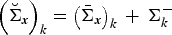 $\left(\breve{\bi \Sigma}_{\bi x} \right)_k = \left( \bar{\bi \Sigma}_{\bi x} \right)_k \,+ \,{\bi \Sigma}_k^ - $
, |·| denotes the absolute value, and c is a scale constant,
 $c \in \left[\matrix{1\!\cdot\!5 &3\!\cdot\!0} \right]$
. Here c is empirically set to 1·5.
3.3. Summary of the new algorithm
The proposed robust adaptive algorithm can be summarised as follows:
-
2 Robust Estimation of Position: performed using Equations (17)–(19).
-
3 Adaptive Kinematic Noise VCV Tuning Matrix Calculation: entries of the tuning matrix
 ${\bi S}_{k - 1}$
are obtained using Equation (23).
-
4 Measurement Update:
(24)
$${\bi X}_k^ + = {\bi X}_k^ - + \bar{\bi K}_k\left( {{\bi y}_k - {\bi h}\left( {{\bi X}_k^ -} \right)} \right)$$
(25)
$${\bi \Sigma} _k^ + = \left( {{\bi I} - { \bar{\bi K}}_k{\bi H}_k} \right){\bi \Sigma} _k^ - $$
(26)
$$ \bar{\bi K}_k = \bar{\bi \Sigma} _k^ - {\bi H}_k\left( {{\bi H}_k \bar{\bi \Sigma} _k^ - {\bi H}_k^T + { \bar{\bi R}}_k} \right)^{ - 1}$$


With
 $${\bi y}_k = {\bi D} \cdot {\bi y}_{s,k}, \bar{\bi R}_k = {\bi D} \cdot \bar{\bi R}_{k,s} \cdot {\bi D}^T$$
where
 ${\bi D}$
is the difference operator that transforms the single-differenced data to double-difference data.
4. TEST COMPUTATION AND ANALYSIS
We now employ real GPS data to demonstrate the efficiency of the proposed Kalman filter. These data describe the relative positioning between a static receiver and a transmitter mounted on an aeroplane. To compare the performance of the new robust, adaptive Kalman filter with that of a classical one, we analyse three cases with/without abrupt changes and/or simulated outliers.
4.1. Outline of test description and data processing schemes
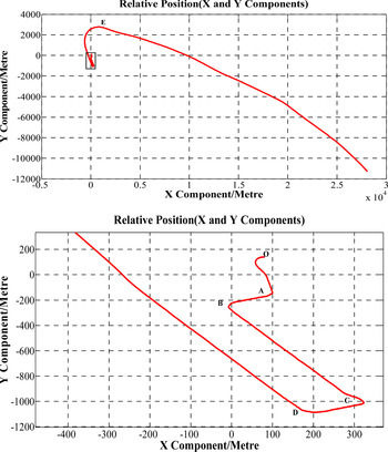
The distance between the rover and the static reference receivers was initially set to about 180 m. The observation session, lasting about 5 h 15 min, was conducted on 12 May 2005, using a sampling rate of 1 Hz. Only the first 2,000 epochs of data were used. In this process, the aeroplane was static for about 1,000 epochs, and then slowly accelerated toward the take-off lane. During this time, the plane stopped for three short periods. After reaching the take-off lane, the plane accelerated to take off. This routine is shown in Figure 1. From the two subfigures, it can be seen that there are abrupt changes that cannot be satisfactorily described by the kinematic model. We expect the proposed adaptive algorithm to handle these cases. In addition, to test the robustness of the new algorithm, outliers of 5 m were added to randomly selected observations in various epochs.
X and Y components of the aeroplane trace relative to the static reference station. Bottom panel: magnification of boxed part. The abrupt changes occur at points O, A, B, C, and D in this figure, and at point E in the top panel.

Furthermore, the carrier observations were used in posterior mode to calculate the relative position, and the results acted as the reference. This is because the carrier observation is much more accurate than the code observation if the ambiguities are fixed correctly.
The performance of the proposed Robust Adaptive Kalman Filtering (New RAF) and the classical method (Classical Kalman Filter – CKF) were compared under the following three scenarios: 1. Abnormal changes without observation outliers; 2. Abnormal changes with observation outliers that do not occur simultaneously; and 3. Abnormal changes and observation outliers that occur simultaneously. The methods were both initialised with a carrier-smoothed code algorithm (Wang et al., Reference Wang, Ou and Guo2007) for 40 epochs to obtain a precise start. To alleviate noise induced by multi-paths and other error sources related to signal path elevation, the diagonal elements of the un-differenced VCV matrix were determined from the elevation angle as follows:
 $${\bi \Sigma} _{ii} = \left[ {\csc \left( {{\bi \beta} _i} \right)} \right]^2$$
where
 ${\bi \beta} _i$
is the elevation angle of the i-th GPS satellite and
 $\csc \left(\bf \cdot \right)$
is the cosecant function.
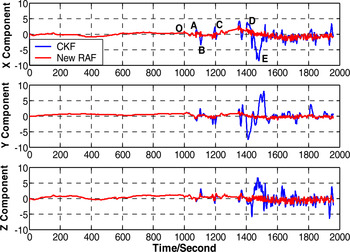
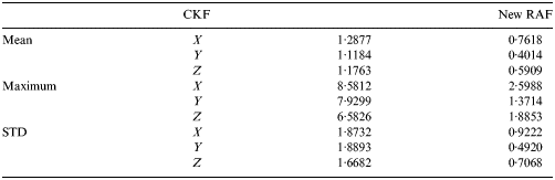
Case 1: The data processing results for abrupt changes without outliers are shown in Figure 2 and Table 1, respectively.
Baseline component errors without outliers. The blue line shows CKF, and the red line denotes the proposed New RAF. Points O, A, B, C, D, and E are the turning points denoted in Figure 1.

Statistical characteristics of the absolute error (m) of CKF and New RAF.

As indicated in Figure 2 and Table 1, the adaptive algorithm was utilised when abrupt changes occurred, i.e., at turning points A, B, C, D, and E.
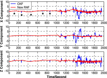
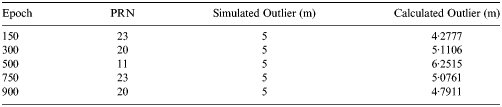
Case 2: Outliers of 5 m were added to a randomly selected GPS satellite code observation at epochs 150, 300, 500, 750, and 900. In this scenario, there were no abnormal changes to test the performance of the robust algorithm. The baseline results are shown in Figure 3, and the outlier detection results are summarised in Table 2.
Baseline component errors with outliers. The observations at epochs marked “★” were contaminated by outliers.

Outlier detection results with QUAD.

From Figure 3 and Table 2, it can be seen that CKF was more sensitive to outliers than the QUAD-based Kalman filter. All the simulated outliers were discerned and recovered with acceptable accuracy.
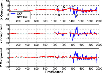
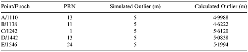
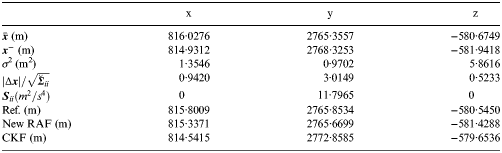
Case 3: An outlier of 5 m was added to a randomly selected GPS satellite code observation at turning points A, B, C, D, and E to validate the efficiency of New RAF when outliers and abrupt changes occur simultaneously. Figure 4 and Table 3 present the results of this experiment. The detailed results obtained by the proposed algorithm according to the processing procedure for point E, as an example, are listed in Table 4.
Baseline component errors with both outliers and abrupt changes. A, B, C, D, and E are the turning points, at which outliers were simultaneously applied.

Outlier Detection Results with QUAD.

Detailed results of New RAF for point E.

From Figure 4 and Table 3, we can conclude that the new robust adaptive algorithm not only resists observation outliers, but also handles abnormal changes, even when these two types of gross error occur simultaneously.
5. ANALYSIS
From Figure 2 and Table 1, we can see that the robust adaptive algorithm works as well as CKF when there are no outliers or abrupt movement state change. Once outliers or abrupt changes were introduced, the algorithm outperformed CKF. Figures 2–4 reveal that regardless of whether observation outliers and abrupt changes occurred alone or together, the proposed robust adaptive algorithm produced satisfactory results.
However, the algorithm requires further improvements. For example, the abnormal movement change at point “O” was not correctly detected, and some of the disagreements between the recovered outliers and the simulated ones were slightly too large. The former problem is caused by the fact that the abrupt movement change at “O” was too lazy to be detected at the adaptive sensitivity level. The latter issue results from improper selection of the QAOs, i.e., some non-contaminated observations were not applied to estimate the outliers. Furthermore, a comparison between traditional robust adaptive filtering and the proposed algorithm should be performed and analysed.
6. CONCLUSION AND DISCUSSION
We have proposed an adaptive algorithm combined with the QUAD robust estimation method. The most attractive aspect of the algorithm is that it can deal with both observation outliers and abrupt movement changes, even when they occur simultaneously. The proposed approach can be divided into two characteristic parts: robust QUAD-based estimation, which uses the current observation to obtain robust estimates of position components and the corresponding equivalent weight factor matrix, and adaptive estimation, which uses the difference between the robust estimates of position components and the predicted position to calculate the kinematic noise VCV tuning matrix. The proposed algorithm proceeds as follows: 1. Time update of the filtering states and the corresponding VCV matrix; 2. Robust estimation of position components; 3. Adaptive kinematic noise VCV tuning matrix estimation based on the previous step; and 4. Combination of robust and adaptive results to update the filtering states and the corresponding VCV matrix. What distinguishes the proposed adaptive algorithm from traditional ones is that it adopts an additive component-wise noise VCV matrix, rather than an adaptive scale factor, to inflate the time-update VCV matrix.
The performance of the proposed method was verified by a set of kinematic GPS positioning data. The proposed method successfully detected observation outliers and abrupt movement changes in three typical cases. These constants, which were empirically determined in this study, require further attention. Their values may differ for different applications. The adaptive estimation of VCV matrices for both observation and kinematic systems is also critical, as they are the foundation of the proposed robust adaptive algorithm.
ACKNOWLEDGMENTS
We would like to thank the reviewers for suggestions that improved this paper. This research is supported by the National Natural Science Foundation of China (Grant Nos. 41374043, 41004005, 41074013), the National Oceanic Commonweal Research Project (Grant No. 201105001) and National Key Scientific Instrument and Equipment Development Project (Grant No. 2011YQ120045). The authors would thank Dr. Guochang Xu of GeoForschungsZentrum (GFZ) Potsdam for providing the kinematic GPS data.
APPENDIX: DERIVATION OF THE DIAGONAL ADAPTIVE KINEMATIC NOISE VCV TUNING MATRIX.
Because a high-sampling-rate receiver is used in the kinematic case, movement can be described by a constant velocity or acceleration model. We use a constant velocity model to derive the new algorithm, assuming the Kalman filter being linearized is defined by Equations (1)–(7), with Equations (13)–(16). In the following derivation, the subscript k is neglected for simplicity.
Assume that the robust estimation of the position components is
 $ \bar{\bi x}$
and its VCV matrix is
 $ \bar{\bi \Sigma} _{\bi x}$
, and let the predicted position components and their VCV matrix be denoted by
 ${\bi x}^ - $
and
 ${\bi \Sigma} _{\bi x}^ - $
, respectively. We construct the statistic
 $$\Delta {\bi x} = \bar{\bi x} - {\bi x}^ -. $$
As
 $ \bar{\bi x}$
and
 ${\bi x}^ - $
are independent, the VCV matrix of
 $\Delta {\bi x}$
is
 ${\bi \Sigma} _{\Delta {\bi x}} = \bar{\bi \Sigma} _{\bi x} + {\bi \Sigma} _{\bi x}^ - $
, according to the error propagation law. If there are any abnormal changes, it is assumed that the kinematic noise VCV matrix will be inflated to
 ${\bi Q} + {\bi S}$
. Then,
 $${\bi \Sigma} _{\Delta {\bi x}} = \bar{\bi \Sigma} _{\bi x} + {\bi \Sigma} _{\bi x}^ - + {\bi \Gamma} _{\bi X}{\bi S}\left( {{\bi \Gamma} _{\bi X}} \right)^T$$
where
 ${\bi S}$
is the tuning matrix that absorbs abnormal changes and
 ${\bi \Gamma} _{\bi X}$
is the kinematic noise coupling matrix. For simplicity,
 ${\bi S}$
is assumed to be diagonal. Let the first two terms on the right-hand side of equation (A2) be denoted as
 $$\breve{\bi \Sigma}_{\bi x} = \bar{\bi \Sigma} _{\bi x} + {\bi \Sigma} _{\bi x}^ -. $$
Then,
 $${\bi \Sigma} _{\Delta {\bi x}} = \breve{\bi \Sigma}_{\bi x} + {\bi \Gamma} _{\bi X}{\bi S}\left( {{\bi \Gamma} _{\bi X}} \right)^T.$$
Taking the assumption and the form of
 ${\bi \Gamma} _{\bi X}$
into account, the i-th diagonal entry of
 ${\bi \Sigma} _{\Delta {\bi x}}$
is
 $$\eqalign{\left({\bi \Sigma}_{\Delta {\bi x}} \right)_{ii} &= \left(\breve{\bi \Sigma}_{\bi x} \right)_{ii} \,+\, \left({\bi \Gamma S} {\bi \Gamma}^T \right)_{ii} \cr &= \left(\breve{\bi \Sigma}_{\bi x} \right)_{ii} \,+\, \displaystyle{1 \over 4} \left(\Delta t \right)^4 {\bi S}_{ii}} \quad (i = 1,2,3).$$
If the standardized statistic
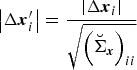 $\left\vert \Delta {\bi x}_i^{\prime} \right\vert = \displaystyle{\left\vert \Delta {\bi x}_i \right\vert \over \sqrt{\left(\breve{\bi \Sigma}_{\bi x} \right)_{ii}}} $
is significantly large, we consider abrupt movement changes to have occurred. Then, the kinematic noise VCV matrix is inflated (Koch and Yang, Reference Koch and Yang1998; Yang et al., Reference Yang, He and Xu2001) as follows:
 $$\eqalign{\left({\bi \Sigma}_{\Delta {\bi x}} \right)_{ii} &= \left(\breve{\bi \Sigma}_{\bi x} \right)_{ii} \displaystyle{\left \vert \Delta {\bi x}_i^{\prime} \right\vert \over c} \cr &= \left(\breve{\bi \Sigma}_{\bi x} \right)_{ii} \,+ \displaystyle{1 \over 4} \left(\Delta t \right)^4{\bi S}_{ii} \cr &\quad {\rm if} \displaystyle{\left\vert \Delta {\bi x}_i \right\vert \over \sqrt{\left(\breve{\bi \Sigma} _{\bi x} \right)_{ii}}} \gt c\comma} $$
where c ∈ [1·5, 3] is an experimental constant.
Then,
 $${\bi S}_{ii} = \left\{\matrix{\displaystyle{4 \over {{\left( {\Delta t} \right)}^4}}\left(\displaystyle{\left\vert \Delta {\bi x}_i^{\prime} \right\vert \over c} - 1 \right) \left(\breve{\bi \Sigma}_{\bi x} \right)_{ii}\comma\ \left\vert \Delta {\bi x}_i^{\prime} \right\vert = \displaystyle{\left\vert \Delta {\bi x}_i \right \vert \over \sqrt{\left(\breve{\bi \Sigma} _{\bi x}\right)_{ii}}} \gt c \cr 0,\hfill &\hskip-6.5pc{\rm otherwise} } \right.$$
Thus, we have derived the diagonal adaptive kinematic noise VCV tuning matrix
 ${\bi S}$
. As denoted by Equation (18), the predicted VCV matrix of both the position and velocity components would be adaptively updated.