2. PRIORS FOR MINIMAX PREDICTIVE ESTIMATION

In this section, we develop general conditions on π for

in (6) to uniformly dominate

in (5) under KL risk (4). The minimaxity of such

will then follow immediately from the minimaxity of

.

We begin by establishing some convenient notation. As indicated previously, we use

to denote the least squares estimate of β based on x. Although y is not observed, it will be useful to use

to denote the least squares estimate of β based on x and y. Note that

and

, where for notational convenience throughout we let Σ_A = (A′A)⁻¹ and Σ_C = (C′C)⁻¹. It will also be useful to let

and

denote the corresponding residual sums of squares (RSS). In terms of this notation, we have the following result.

LEMMA 1. The uniform prior predictive estimate

in (5) can be expressed as

where Ψ = I + BΣ_AB′. Moreover, the KL risk of

is uniformly smaller than that of the plug-in estimator

.

Proof. Because

, the posterior of β under the uniform prior is

. It follows that the posterior of Bβ is

, and thus the predictive estimator is

To calculate the risk of

, let

denote the hat matrix based on x and

denote the hat matrix based on both x and y. It is easy to see that

where e₁,…,e_p are the eigenvalues of (A′A)⁻¹B′B. Moreover,

That

dominates

follows from the fact that log(x + 1) ≤ x for any x > 0. █

Risk comparisons of a Bayes predictive density

with

are greatly facilitated by the following representation of

in terms of

. An analogous representation of the posterior mean in terms of the maximum likelihood estimator (MLE), which simplifies multivariate normal mean estimation under quadratic risk, was proposed by Brown (1971). For our representation, it will be useful to denote the marginal distribution of Z|β ∼ N_p(β,Σ) under π by

Thus, the marginal distributions of

and

under π are denoted by

and

, respectively.

LEMMA 2. If m_π(z;Σ) is finite for all z and Σ, then

is a proper probability distribution. Furthermore, it can be expressed as

where

is defined by (8).

Proof. When m_π(z;Σ) is finite for all z and Σ, that

is a proper probability distribution follows from integrating with respect to y and switching the order of integration.

Next, straightforward calculation yields

Similarly, we obtain

The representation (10) follows immediately from (6), (11), and (12). █

The next result provides a representation of the difference between the KL risks of

and

in terms of the marginal distributions of

and

.

LEMMA 3. The difference between the KL risks of

and

is given by

where E_β,Σ(·) stands for expectation with respect to the N_p(β,Σ) distribution.

Proof. The KL risk difference between

and

can be expressed as

where the last equality follows from Lemma 2. The result then follows from the change of variable theorem. █

To exploit the representation (13), we proceed to transform the distributions to canonical form. Because Σ_A and Σ_C are both symmetric and positive definite, there exists an invertible p × p matrix W such that

where

Because Σ_C = (C′C)⁻¹ = (A′A + B′B)⁻¹ and B′B is nonnegative definite, d_i ∈ (0,1] for all 1 ≤ i ≤ p with at least one d_i < 1. Finally, let μ = W⁻¹β,

, and

, so that

LEMMA 4. Let π_W(μ) = π(Wμ). Then, the difference between the KL risks of

and

is given by

where E_μ,Σ(·) stands for expectation with respect to the N_p(μ,Σ) distribution.

Proof. The result follows by transforming the expressions in Lemma 3:

Similarly,

Thus, (17) equals (13). █

We now proceed to find conditions on m_π for which the risk difference (17) is nonnegative for all μ. Because

is minimax, this will then imply that

is minimax under the prior π corresponding to π_W. Now for w ∈ [0,1], let

where Σ_D is defined as in (15). Next, for Z ∼ N_p(μ,V_w), let

Thus, we may rewrite (17) as

Because h_μ(w) is continuous in w, it suffices to derive conditions on m_π such that (∂/∂w)h_μ(w) < 0 for all μ and w ∈ [0,1]. Letting v_i be the ith diagonal element of V_w, we have by the chain rule

The following result provides unbiased estimates of the components of (21) that, when combined with (17), will be seen to play a key role in establishing sufficient conditions on m_π for

to be minimax and to dominate

. As noted by George et al. (2006), these estimates are very similar to the unbiased estimates of risk for the estimation of a multivariate mean under squared error loss; see Stein (1974, 1981).

LEMMA 5. If m_πW(z;I) is finite for all z, then for any 0 ≤ w ≤ 1, m_πW(z;V_w) is finite. Moreover,

Proof. When m_πW(z;I) is finite for all z, it is easy to check that for any fixed z and any 0 ≤ w ≤ 1,

Next, letting Z* = V_w^−1/2(Z − μ) ∼ N(0,I), we have

where

Making use of the well-known univariate heat equation

(see, e.g., Steele, 2001, and the Brown, 1971, representation E_π(μ_i′|z_i) = z_i + v_i(∂/∂z_i)log m_πW(z)), (22) and (23) can be verified via the same steps as in the proof of Lemma 3 in George et al. (2006). █

Now we can obtain sufficient conditions for a Bayes procedure

to be minimax by combining (20), (21), and Lemma 5. The following result provides a substantial generalization of Theorem 1 of George et al. (2006).

THEOREM 1. Suppose that m_π(z;WW′) is finite for all z with the invertible matrix W defined as in (14). Let H(f(z₁,…,z_p)) be the Hessian matrix of f.

(i) If trace{H(m_π(z;WV_wW′))[Σ_A − Σ_C]} ≤ 0 for all w ∈ [0,1], then

is minimax under R_KL. Furthermore,

dominates

unless π = π_U.

(ii) If

for all w ∈ [0,1], then

is minimax under R_KL. Furthermore,

dominates

if for all w ∈ [0,1], this inequality is strict on a set of positive Lebesgue measure.

Proof. To prove the minimaxity of

under R_KL, it suffices to show that (22) or (23) is nonpositive because by (21) that would imply the nonnegativity of (20). Dominance would further follow by showing that (22) or (23) is also strictly negative on a set of positive Lebesgue measure.

Noting that m_πW(z;V_w) = m_π(Wz;WV_wW′), and letting

, we obtain

Similarly,

Now (i) and (ii) follow immediately from (22), (23), (26), and (27). █

The next result follows using the fact that (∂²/∂z_i²)m_πW(z;V_w) ≤ 0 when (∂²/∂μ_i²)π_W(μ) ≤ 0.

COROLLARY 1. Suppose that m_π(z;WW′) is finite for all z. Then

will be minimax if

Furthermore,

will dominate

unless π = π_U.

Example (Scaled harmonic prior)

Suppose that A = B. In this case,

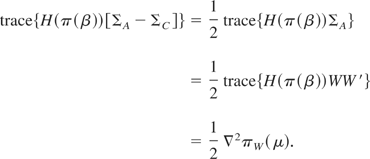
Let π_W(μ) ∝ ∥μ∥^−(p−2) when p ≥ 3 and π_W(μ) ∝ 1 when p < 3. Note that π_W is harmonic, i.e., ∇²π_W(μ) ≡ 0, and not equal to π_U when p ≥ 3. For p ≥ 3, the corresponding prior on β is a “scaled harmonic prior”

where η₁,…,η_p > 0 are the eigenvalues of Σ_A and for p < 3, π(β) ∝ 1. (The expression (29) is obtained using the fact that there exists an orthonormal matrix O such that W = O diag(η₁^1/2,…,η_p^1/2)O′.) By Corollary 1 and (28), the predictive estimator

under this prior is minimax and dominates

when p ≥ 3. It is easy to check that these results hold when A = rB for any known constant r.

3. PREDICTIVE DENSITY ESTIMATION NEAR SUBSET MODELS

When a prior centered at 0 such as the scaled harmonic prior (29) is applied to β, the risk reduction of

over

is greatest when all the components of β are close to 0. Thus, it would be sensible to use this prior if it was felt that all p predictors in A and B were potentially irrelevant. However, such a prior would be ineffectual if only a subset of the p predictors were irrelevant, in other words, if only a subset of the β components were close to 0. In this section, we extend our results for the setting where such a subset is known. This will set the stage for Section 4, where we develop new results for the more realistic model uncertainty setting where such a subset is unknown.

Let S be the subset of {1,…,p} corresponding to the indices of the potentially irrelevant predictors and let q_S = |S| be the number of elements in S. Let β_S be the subvector of β corresponding to the columns of A indexed by S. Similarly, let

and

be the subvectors of

and

, respectively, corresponding to β_S. Finally, for notational convenience, let Σ_A,S and Σ_C,S be the submatrices of Σ_A and Σ_C, respectively, which are the covariance matrices of

and

.

When only the elements of β_S are thought to be close to zero, it would be sensible to consider a prior that is uniform on β_S, where S is the complement of S. We denote such a prior by π_S and let π_S* be the restriction of π_S to β_S so that

is a function of β_S only. To exploit the possibility that β_S is close to zero, π_S* would then be centered around 0.

LEMMA 6. If m_πS(z;Σ) is finite for all z and Σ, then

is a proper probability distribution. Furthermore, it can be expressed as

where

is defined by (8).

Proof. The first assertion was proved in Lemma 2. Next, proceeding as in the derivation of (11), we obtain

Similarly, we obtain

The representation (31) follows immediately from (6), (32), and (33). █

The following results provide sufficient conditions for the minimaxity of

and for its dominance over

. We omit the proofs, which are obtained using the same arguments leading to Theorem 1 and Corollary 1. Analogously to our previous development there, we let W_S be an invertible q_S × q_S matrix such that Σ_A,S = W_SW_S′ and Σ_C,S = WΣ_D,SW′, where Σ_D,S = diag(d₁,…,d_qS) as in (15). Finally, let V_S,w = wI + (1 − w)Σ_D as in (18).

THEOREM 2. Suppose that m_πS*(z;W_SW_S′) is finite for all z. Let H(f(z₁,…z_qS)) be the Hessian matrix of f.

(i) If trace{H(m_πS*(z;W_SV_S,wW_S′))[Σ_A,S − Σ_C,S]} ≤ 0 for all w ∈ [0,1], then

is minimax under R_KL. Furthermore,

dominates

unless π_S = π_U.

(ii) If

for all w ∈ [0,1], then

is minimax under R_KL. Furthermore,

dominates

if for all w ∈ [0,1], this inequality is strict on a set of positive Lebesgue measure.

COROLLARY 2. Suppose that m_πS*(z;W_SW_S′) is finite for all z. Then

will be minimax if

Furthermore,

will dominate

unless π_S = π_U.

Example (continued) (Scaled harmonic prior)

Suppose that A = B so that as in (28),

where μ_S = W_S⁻¹β_S. Here let π_WS(μ) ∝ ∥μ_S∥^−(q_S−2) when q_S ≥ 3 and π_W(μ_S) ∝ 1 when q_S < 3. As before, π_WS is harmonic, i.e., ∇²π_WS(μ) ≡ 0, and not equal to π_U when q_S ≥ 3. For q_S ≥ 3, the corresponding scaled harmonic prior on β is

where η₁,…,η_qS > 0 are the eigenvalues of Σ_A,S and for q_S < 3, π_S(β) ∝ 1. By Corollary 2 and (34),

here is minimax and dominates

when q_S ≥ 3.

4. MINIMAX MULTIPLE SHRINKAGE PREDICTIVE ESTIMATION

We consider the more realistic model uncertainty setting where there is uncertainty about which subset of the p predictors in A and B should be included in the model. For each choice of S, we have obtained general sufficient conditions for

to be minimax and to dominate π_U. However, such

will only offer meaningful risk reduction when β is near the region where π_S is largest. For example, under the scaled harmonic prior in (35), such risk reduction occurs when β_S is close to 0. The difficulty then is how to proceed when the subset of irrelevant predictors indexed by S is unknown. Rather than arbitrarily selecting S, an attractive alternative is to use a multiple shrinkage predictive estimator that uses the data to adaptively emulate the most effective

.

The multiple shrinkage procedure here is obtained by using a finite mixture of the contemplated priors. A similar multiple shrinkage construction for parameter estimation under squared error loss was proposed and developed by George (1986a, 1986b, 1986c). Let Ω be the set of all the subsets S under consideration, possibly even the set of all possible subsets. For each S ∈ Ω, let π_S be the designated prior of the form (30) on β and assign it probability w_S ∈ [0,1] such that [sum ]_S∈Ωw_S = 1. Thus we construct the mixture prior

This prior yields the multiple shrinkage predictive estimator

Here each

is given by (31) in Lemma 6, and each posterior probability is of the form

which follows from (32).

The form (37) reveals

to be an adaptive convex combination of the individual shrinkage predictive estimates

. Note that through

,

doubly shrinks

by putting more weight on the

for which m_πS* is largest and hence

is shrinking most. Thus, we expect

to offer meaningful risk reduction whenever β_S is near the region where π_S is largest for any S ∈ Ω. For example, if every π_S in π* is one of the scaled harmonic priors in (35), such risk reduction occurs when β_S is close to 0 for any S ∈ Ω for which q_S ≥ 3. Thus, the potential for risk reduction using

is far greater than the risk reduction using an arbitrarily chosen

.

We should also note that the allocation of risk reduction by

is in part determined by the w_S weights in (38). Because each

is so adaptive through m_πS*, choosing the weights to be uniform should be adequate. However, one may also want to consider some of the more refined suggestions for choosing such weights for the multiple shrinkage estimators in George (1986b).

The potential for a multiple shrinkage

to offer meaningful risk reduction in many different regions of the parameter space is greatly enhanced when it is minimax and therefore can only improve on the “noninformative” minimax

. The following two results show that such minimaxity and dominance of

can be obtained. We then conclude with an explicit example of such domination.

THEOREM 3. Suppose for all S ∈ Ω, m_πS*(z;W_SW_S′) is finite for all z. Let H(f(z₁,…,z_qS)) be the Hessian matrix of f. If for all S ∈ Ω,

then

in (37) is minimax under R_KL. Furthermore,

dominates

unless π* = π_U.

Proof. From (31), (37), and (38), it is straightforward to show that

can be reexpressed as

Because p* is of the same form as

in (31), namely, a ratio of marginals times

, we can apply the same arguments leading to the proofs of Theorems 1 and 2. These steps show that a sufficient condition for the minimaxity and dominance claims is

This condition is implied if (39) holds for all S ∈ Ω. █

The next result follows using the same argument leading to Corollaries 1 and 2.

COROLLARY 3. Suppose for all S ∈ Ω, m_πS*(z;W_SW_S′) is finite for all z. Then

in (37) will be minimax if for all S ∈ Ω

Furthermore,

will dominate

unless π = π_U.

Example (continued) (Scaled harmonic prior)

For each S ∈ Ω, let π_S(β) be the scaled harmonic prior given by (35) when q_S ≥ 3 and by π_S(β) ∝ 1 when q_S < 3. When A = B, by Corollary 3,

under these priors will be minimax and will dominate

if q_S ≥ 3 for at least one S ∈ Ω.

5. PREDICTIVE DENSITY ESTIMATION NEAR LINEAR SUBSPACES

The harmonic prior predictive estimator

described in Section 3 and incorporated into the multiple shrinkage predictive estimators

in Section 4 offers risk reduction in the region of the parameter space where β_S is close to 0. This can be seen as a special case of the following general construction of a predictive estimator that obtains risk reduction when β is close to a linear subspace of R^p.

Suppose one would like to obtain a predictive density estimator with greatest risk reduction in the region where β is close to a linear subspace G ⊂ R^p. In the case of

, G would be the subspace of all β ∈ R^p for which β_S ≡ 0. Alternately, if risk reduction was desired, say, when the components of β were close to equal, then one would consider G = [1], the subspace spanned by (1,…,1)′. Let P_Gβ ≡ argmin_g∈G∥β − g∥ be the projection of β onto G and define β_G ≡ (I − P_G)β to be the projection of β onto the orthogonal complement of G. For the construction of

in Section 3, β_G = β_S. For G = [1], β_G = (β − β) where β is the vector of components all equal to

.

The main idea behind the general construction is to use a prior that leads to shrinkage of β_G toward 0 while leaving the remainder of β untouched. This can be obtained by using a prior of the form

which is effectively uniform on (β − β_G). This is a special case of the prior over β_S in (30). Note that because β_G is q_G ≡ (p − dim(G)) dimensional, π_G* is a function from R^q_G to R.

Analogous to the construction in Lemma 6, predictive density estimators

corresponding to priors of the form π_G in (41) can be expressed as

where

is defined by (8),

and

are the projections of

and

onto the orthogonal complement of G, respectively, and Σ_A,G and Σ_C,G are the covariance matrices of

and

, respectively. It is straightforward to see that Theorem 2 and Corollary 2 and their proofs can be extended to obtain conditions on π_G*(β_G) for such

to be minimax and to dominate

. (Simply substitute the symbol G for the symbol S throughout.)

Example (continued)

Extending (35), consider the following scaled harmonic prior on β. For q_G ≥ 3, let

where η₁,…,η_qG > 0 are the eigenvalues of Σ_A,G, and for q_G < 3, let π_G(β) ∝ 1. Note that when q_G ≥ 3 the resulting

shrinks

toward G, offering reduced risk when β is close to G. By the extension of Corollary 2, such

will be minimax and dominate

when A = B and q_G ≥ 3.

Finally, following the development in Section 4 one can easily incorporate such

into multiple shrinkage predictor estimators

. Letting Ω be a set of subspaces G under consideration, construct the mixture prior

where for each G ∈ Ω, π_G is the designated prior of the form (41) and w_G ∈ [0,1] is such that [sum ]_G∈Ωw_G = 1. This prior yields the multiple shrinkage predictive estimator

where each

is given by (42) and each posterior probability is of the form

Here,

is an adaptive convex combination of the individual shrinkage predictive estimates

and offers risk reduction whenever β_G is near the region where π_G is largest for any G ∈ Ω. Thus, the potential for risk reduction using

is far greater than the risk reduction using an arbitrarily chosen

. It is straightforward to see that Theorem 3 and Corollary 3 and their proofs can be extended to get conditions for such

to be minimax and dominate

. (Simply substitute the symbol G for the symbol S throughout.)

Example (continued) (Scaled harmonic prior)

For each G ∈ Ω, let π_G(β) be the scaled harmonic prior given by (43) when q_G ≥ 3 and by π_G(β) ∝ 1 when q_G < 3. When A = B, by the extension of Corollary 3,

for these priors will be minimax and will dominate

if q_G ≥ 3 for at least one G ∈ Ω.