2.1. Set-up

We perform new experiments using the two-dimensional set-up illustrated in figure 1(a) and described in detail in Robbe-Saule et al. (Reference Robbe-Saule, Morize, Henaff, Bertho, Sauret and Gondret2021). A rectangular tank of length $L=2\ \textrm {m}$ and transverse width $W=0.15\ \textrm {m}$ is filled up to a height $h_0$ with initially still water. On the left-hand side of the tank, a rectangular granular column of height $H_0$ and length $L_0$ stands on a solid step of height $h_0$ so that the grains, initially retained by a vertical gate, are just above the water interface. The granular material consists of monodisperse glass beads of diameter $5$ mm and density $\rho = 2.5\ \textrm {g}\,\textrm {cm}^{-3}$. Images are taken by a camera from the sidewall of the tank. The water is dyed with fluorescein to enhance the contrast and facilitate the processing of the time evolution of the free surface of the water and of the grains.

Figure 1.

Sketch of the experimental set-up (a) in the initial configuration, with a dry granular column of height $H_0$ and length $L_0$ above a water depth $h_0$, and (b) during the granular collapse, with an advancing front $x_f(t)$ at the water surface and a generated wave of amplitude $A(t)$ and mid-height width $\lambda (t)$.

At time $t=0$, the gate is quickly lifted by a linear motor at 1 m s$^{-1}$. The granular column then collapses into the water, leading to an advancing granular front $x_f(t)$, which generates an impulse wave of amplitude $A(t)$ and mid-height width $\lambda (t)$, as sketched in figure 1(b). We perform systematic experiments, where both the size of the column and the water depth are varied, as detailed in table 1. We explore a large range of aspect ratio $a=H_0/L_0$, initial volume of the column $V_0=H_0L_0W$, and global Froude number ${Fr}_0=\sqrt {H_0/h_0}$, which compares the typical vertical free-fall velocity of the granular medium, $\sqrt {gH_0}$, to the velocity of linear gravity waves in shallow water, $c_0=\sqrt {gh_0}$.

Table 1.

Sets of experimental parameters with corresponding data symbols.

2.2. Description of the observed regimes of nonlinear waves

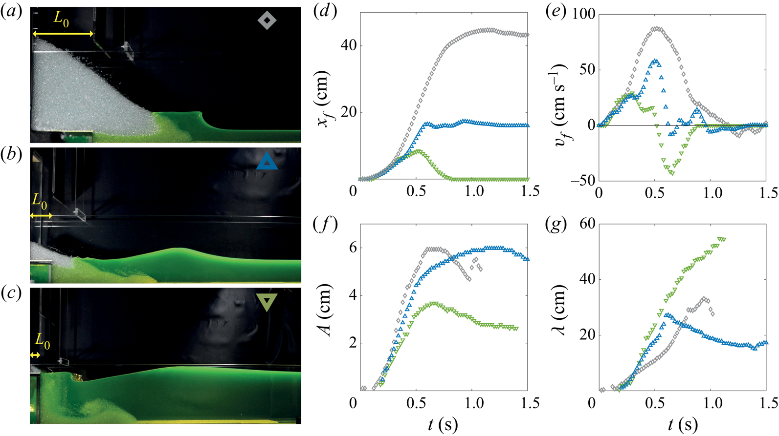
Depending on the geometry of the granular columns and the water depth, leading to different global Froude number ${Fr}_0$, we observe three different regimes of nonlinear waves (see figure 2(a–c), and supplementary movies available at https://doi.org/10.1017/jfm.2021.400). At large ${Fr}_0$, strong asymmetric waves are generated with the shape of transient positive surges or bores, as shown in figure 2(a). The wave generated systematically breaks in the near-field region, and corresponds to the plunging breaker reported in Robbe-Saule et al. (Reference Robbe-Saule, Morize, Henaff, Bertho, Sauret and Gondret2021). At moderate ${Fr}_0$, quasi-symmetrical waves are generated, consisting of a unique main pulse of soliton-like shape, as reported in figure 2(b). This wave may break or not depending on its relative amplitude $A/h_0$. The breaking cases at high $A/h_0$ correspond to spilling breakers (Robbe-Saule et al. Reference Robbe-Saule, Morize, Henaff, Bertho, Sauret and Gondret2021). At low ${Fr}_0$, waves with slightly reversed asymmetry and strong unsteadiness are generated (see figure 2c). This situation corresponds to the nonlinear transition waves reported by Fritz et al. (Reference Fritz, Hager and Minor2004) and Viroulet et al. (Reference Viroulet, Cébron, Kimmoun and Kharif2013).

Figure 2.

(a–c) Photographs of the different wave shapes observed: (a) bore wave at $H_0 = 39\ \textrm {cm}$, $L_0 = 14.5\ \textrm {cm}$, $h_0 = 4\ \textrm {cm}$ (${Fr}_0=3.1$, ${Fr}_f=1.39$); (b) solitary wave at $H_0 = 29\ \textrm {cm}$, $L_0 = 10\ \textrm {cm}$, $h_0 = 8\ \textrm {cm}$ (${Fr}_0=1.9$, ${Fr}_f=0.65$); and (c) nonlinear transition wave at $H_0 = 39\ \textrm {cm}$, $L_0 = 5\ \textrm {cm}$, $h_0 = 25\ \textrm {cm}$ (${Fr}_0=1.2$, ${Fr}_f=0.19$). (d–g) Time series of (d) the position $x_f$ and (e) the velocity $v_f$ of the granular front, and of (f) the amplitude $A$ and (g) the mid-height width $\lambda$ of the wave for the experiments of panels (a) grey $\diamond$, (b) blue $\triangle$, and (c) green $\triangledown$.

Figure 2(d–f) report the time evolution of the granular collapse and of the generated wave for the three examples of figure 2(a–c). At high ${Fr}_0$ (grey $\diamond$), the position of the granular front, $x_{f}(t)$, continually increases from zero to a final maximum value $x_{f_\infty } \gg h_0$ ($x_{f_\infty } \simeq 11 h_0$ in figure 2d). The corresponding velocity of the front $v_f=\mathrm {d}x_{f}/\mathrm {d}t$ exhibits a bell shape from zero up to a maximum value $v_{f_m} \gtrsim \sqrt {gh_0}$ ($v_{f_m} \simeq 1.4 \sqrt {gh_0}$ in figure 2e) and then decreases to zero. Both the amplitude $A$ and the mid-height width $\lambda$ increase during the generation process, until reaching a maximum value $A_m \gtrsim h_0$ with the corresponding $\lambda _m \gg h_0$ ($A_m \simeq 1.5 h_0$ and $\lambda _m \simeq 5 h_0$ in figure 2f,g, respectively), at the moment where the plunging breakup occurs ($t \simeq 0.7\ \textrm {s}$ in figure 2e), which leads to a sudden decrease of $A$.

At moderate ${Fr}_0$ (blue $\triangle$), the time evolution of the granular collapse is similar to that described above but with a smaller maximal extension $x_{f_\infty } \gtrsim h_0$ and a smaller maximum velocity $v_{f_m} \simeq \sqrt {gh_0}$ ($x_{f_\infty } \simeq 2h_0$ and $v_{f_m} \simeq 0.7 \sqrt {gh_0}$ in figure 2d,e, respectively). The wave amplitude increases abruptly first and then more slowly to a maximum value $A_m \simeq h_0$ ($A_m \simeq 0.75 h_0$ in figure 2f) before decreasing due to the breaking of the wave. In the meantime, the width $\lambda$ first grows up to a maximum value, and then decreases down to $\lambda _m > h_0$ ($\lambda _m \simeq 3 h_0$ in figure 2f) when the wave propagates away from the collapse.

At low ${Fr}_0$ (green $\triangledown$), the time evolution of the granular collapse is very different from the two previous situations: $x_{f}$ increases from zero up to a maximum value $x_{f_m} \lesssim h_0$ ($x_{f_m} \simeq 0.3 h_0$ in figure 2d) before decreasing down to zero when the flow rate of the granular medium starts to vanish. In this configuration, the bottom wall does not play a significant role in the granular dynamics. The corresponding velocity $v_{f}(t)$ exhibits first a positive maximum $v_{f_m} < \sqrt {gh_0}$ ($v_{f_m} \simeq 0.2 \sqrt {gh_0}$ in figure 2e), but also a negative minimum at the end of the collapse, corresponding to the receding phase of the granular flow. In the meantime, while the wave amplitude first increases to a maximum value $A_m < h_0$ before slightly decreasing, the mid-height width displays a monotonic growth beyond $\lambda _m \simeq h_0$($A_m \simeq 0.3 h_0$ and $\lambda _m \simeq 1.2 h_0$ in figure 2f,g, respectively), revealing that the wave flattens after its generation. These waves all exhibit a wavelength much larger than the capillary length $\lambda _c \simeq 1.6\ \textrm {cm}$ and larger than the water depth (except for a few experiments that are discussed in § 3.3), so that they correspond to gravity waves in shallow-water conditions.

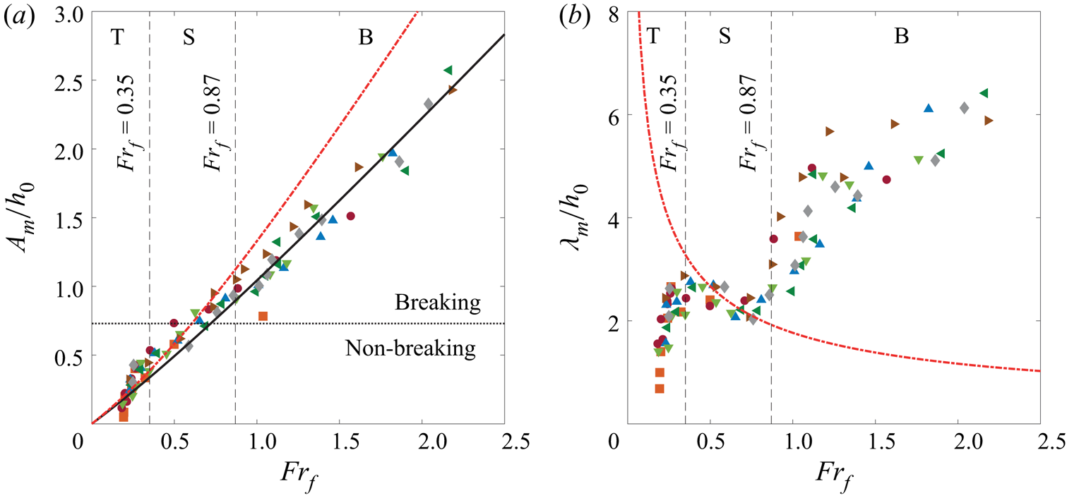
The local Froude number, ${Fr}_f = v_{f_m}/\sqrt {gh_0}$, based on the velocity of the granular front, was found to be the relevant dimensionless parameter to describe the wave generation (Robbe-Saule et al. Reference Robbe-Saule, Morize, Henaff, Bertho, Sauret and Gondret2021). All the experimental results for the maximum wave amplitude $A_m$ and the associated mid-height width $\lambda _m$, non-dimensionalized by the water depth $h_0$, are plotted as a function of ${Fr}_f$ in figure 3(a,b). A monotonic increase of the relative wave amplitude $A_m/h_0$ with ${Fr}_f$ is observed, whereas the relative mid-height width $\lambda _m/h_0$ first increases but then slightly decreases before increasing again. These different behaviours lead to a clear separation of the three wave regimes described above: nonlinear transition waves (T) for ${Fr}_f \lesssim 0.35$, solitary waves (S) for $0.35 \lesssim {Fr}_f \lesssim 0.87$, and transient bore waves (B) for ${Fr}_f \gtrsim 0.87$. In the next section, we characterize the wave regimes using theoretical models adapted to the different regimes and obtain scaling laws for the maximal wave amplitude and the corresponding wavelength with the local Froude number ${Fr}_f$, for regimes S and B.

Figure 3.

(a) Relative amplitude $A_m/h_0$ and (b) mid-height width $\lambda _m/h_0$ of the generated waves as functions of the local Froude number ${Fr}_f$ for all the experiments of table 1, with predictions from (3.3) (black full line) and (3.9) ( red dashed line). The two vertical thin dashed lines at ${Fr}_f = 0.35$ and ${Fr}_f = 0.87$ separate the three regimes corresponding to nonlinear transition waves (T), solitary waves (S) and bore waves (B), respectively. The horizontal dotted line at $A_m/h_0 \simeq 0.73$ separates breaking and non-breaking waves.

3.1. Bore waves

For large values of ${Fr}_f$ (regime B, ${Fr}_f \gtrsim 0.87$), the deformation of the free surface of the water is very similar to a bore or a positive surge during the generation process: the shape is an elongated water bump of height $h_0 + A_B$ with an abrupt step front propagating over the downstream region of height $h_0$. These waves are observed during the collapse of granular columns with a large initial height $H_0$ relative to the water depth $h_0$, and therefore for large ${Fr}_0$. In such conditions, the advancing granular front is almost vertical throughout the entire water depth and acts as a vertical translating piston over a distance $x \gg h_0$ at the velocity $v_p$ (see figure 2a). We consider the mass and momentum conservation equations in the frame of reference of the bore propagating at the velocity $c$:

(3.1)\begin{equation} \left. \begin{gathered} \displaystyle (c-v_p) (h_0+A_B)-c h_0 = 0,\\ \displaystyle (c-v_p)^2(h_0 + A_B)-c^2h_0+\frac{g}{2} [(h_0 + A_B)^2-{h_0}^2 ] =0. \end{gathered} \right\} \end{equation}

These equations describe a stationary hydraulic jump of amplitude $A_B$, separating a thin supercritical region of depth $h_0$ and constant velocity $-c$ from a thick subcritical region of depth $h_0 + A_B$ and of constant velocity $v_p-c$, when assuming no dissipation at the bottom wall and a hydrostatic vertical pressure gradient far enough from the jump (Guyon et al. Reference Guyon, Hulin, Petit and Mitescu2015). Combining these two equations leads to a nonlinear relation between the relative amplitude $A_B/h_0$ and the Froude number ${Fr}_p = v_p/\sqrt {gh_0}$ based on the piston velocity $v_p$:

(3.2)\begin{equation} \frac{A_B}{h_0} \left( \frac{1+A_B/(2h_0)}{1+A_B/h_0} \right)^{1/2}= {Fr}_p. \end{equation}

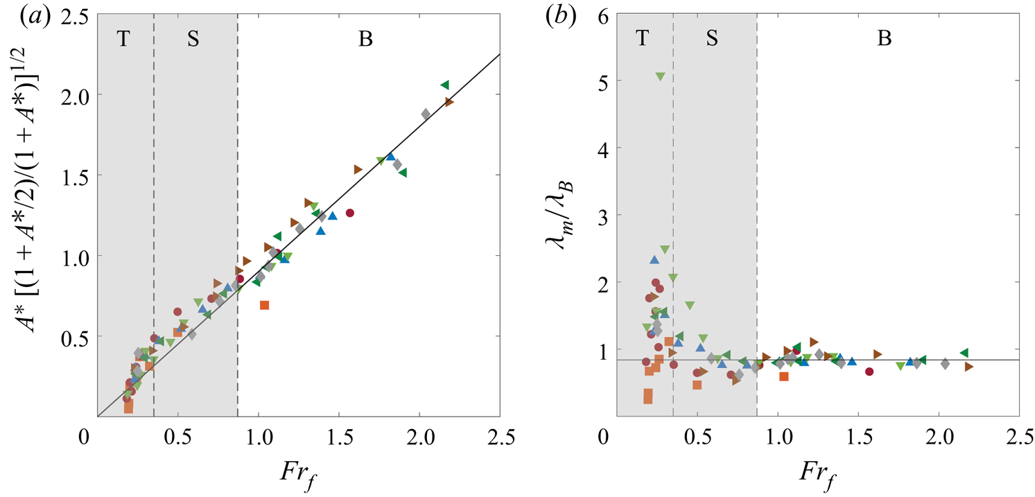
Figure 4(a) shows the rescaled experimental data using the left-hand side of (3.2), with $A_B=A_m$, as a function of ${Fr}_f$. The data corresponding to ${Fr}_f \gtrsim 0.87$ collapse onto a straight line of slope 0.9. Therefore, these nonlinear waves can be seen as bores generated by a solid wall pushing the water at an effective constant velocity $v_p$, a little smaller than the maximal velocity of the granular front $v_{f_m}$. The explicit expression for $A_B/h_0$ as a function of ${Fr}_p$ can be obtained as the only positive solution of the third-order equation (3.2):

(3.3)\begin{align} \frac{A_B}{h_{0}}=\frac{2}{3} \left\{ 2 \sqrt{ 1 + 3{{Fr}_p}^2 /2 }\, \cos\!\left( \frac{1}{3} \cos^{{-}1}\!\left[ \frac{3}{4}\frac{({Fr}_p-2\sqrt{2}/3)({Fr}_p+2\sqrt{2}/3)}{({{Fr}_p}^2+2/3) \sqrt{1 + 3{{Fr}_p}^2 /2 }} \right] \right) - 1 \right\}. \end{align}

Figure 4.

(a) Plot of $A^*[(1+A^*/2)/(1+A^*)]^{1/2}$ as a function of ${Fr}_{f}$ for all the experimental data of table 1, with $A^*=A_m/h_0$, and the best linear fit (full line) with a slope 0.9 for the data corresponding to bore waves (${Fr}_f \gtrsim 0.87$). (b) Ratio of the experimental mid-height width $\lambda _m$ of the wave to the calculated one, $\lambda _B$, from (3.4), as a function of ${Fr}_f$. The horizontal solid line corresponds to $\lambda _m/\lambda _B=0.84$.

The solid line in figure 3(a) corresponds to (3.3) with ${Fr}_p = 0.9 {Fr}_f$. This prediction fits very well the data for ${Fr}_f \gtrsim 0.87$, i.e. in regime B. Note that this nonlinear variation would asymptotically tend to the linear expression $A_B/h_0 \sim \sqrt {2} {Fr}_p$ as ${Fr}_p \rightarrow +\infty$. The wavelength $\lambda _B$ can also be estimated from the mass conservation at the end of the generation of the bore, assuming that the hydraulic jump has the shape of a pure step. Indeed, when the piston has travelled over the total distance $x_p$, we should have

(3.4)\begin{equation} \lambda_B=x_p \frac{h_0}{A_B}. \end{equation}

Figure 4(b) presents the ratio $\lambda _m/\lambda _B$ as a function of ${Fr}_f$. Here, we consider that $x_p$ corresponds to the value of $x_f$ at the end of the wave generation, when $A=A_m$. A plateau is observed with a value $\lambda _m/\lambda _B \simeq 0.84$ for ${Fr}_f \gtrsim 0.87$. Since the hydraulic jump is not a pure step and the granular front is not exactly a vertical advancing wall at a constant velocity, the observed wavelength $\lambda _m$ is indeed a little smaller than the predicted value $\lambda _B$. Note that (3.4) implies that $\lambda _B/h_0 \sim (x_{p}/h_0){{Fr}_f}^{-1}$ at large ${Fr}_f$, where $\lambda _B/h_0$ depends not only on ${Fr}_f$ but also on $x_{p}/h_0$. This explains why the experimental data $\lambda _m/h_0$ of regime B do not collapse onto a master curve in figure 3(b), but are quite dispersed, as they also depend on $x_{f_m}/h_0$.

3.2. Solitary waves

In an intermediate range of local Froude number (regime S, $0.35 \lesssim {Fr}_f \lesssim 0.87$), the generated waves exhibit a solitary-like shape. Solitons are solutions of the Korteweg– de Vries equation valid for shallow-water waves without dissipation (Dauxois & Peyrard Reference Dauxois and Peyrard2006). In that theoretical framework, the free surface elevation $\eta (x,t)$ of a soliton is given by

(3.5a)\begin{equation} \eta(x,t)=A_S \operatorname{sech}^2 \left( \frac{c_{S}t-x}{ \lambda_{S} } \right), \end{equation}

with

(3.5b,c)\begin{equation} \lambda_{S} = 2h_0\sqrt{\frac{h_0}{3A_S}} \quad\mathrm{and}\quad c_{S}=\sqrt{gh_0} \left( 1+\frac{A_S}{2h_0} \right), \end{equation}

where $A_S$, $\lambda _{S}$ and $c_{S}$ are the amplitude, characteristic width and velocity of the wave, respectively, and $\operatorname {sech}$ is the hyperbolic secant function. These solitons can be generated experimentally by wavemakers with a vertical piston moving according to the following law (Goring & Raichlen Reference Goring and Raichlen1980; Synolakis Reference Synolakis1990; Guizien & Barthélemy Reference Guizien and Barthélemy2002):

(3.6)\begin{equation} x_p(t)=\frac{A_S\lambda_{S}}{h_0}\tanh \left( \frac{c_{S}t-x_p(t)}{\lambda_{S}} \right). \end{equation}

Note that, for the experiments in this regime, the time evolution of the granular front $x_f(t)$ is close to a hyperbolic tangent evolution, as shown by the curve in figure 2(d). The maximum value of the time derivative of (3.6) leads to the following equation for the maximum velocity $v_p$ of the piston:

(3.7)\begin{equation} v_p=\frac{A_S}{h_0}(c_{S}-v_p). \end{equation}

Considering the expression (3.5c) for $c_{S}$ together with (3.7) leads to a relation between the relative wave amplitude of the solitary wave $A_S/h_0$ and the Froude number ${Fr}_p$ based on the piston velocity $v_p$:

(3.8)\begin{equation} \frac{A_S}{h_0} \frac{1+A_S/(2h_0)}{1+A_S/h_0}={Fr}_p. \end{equation}

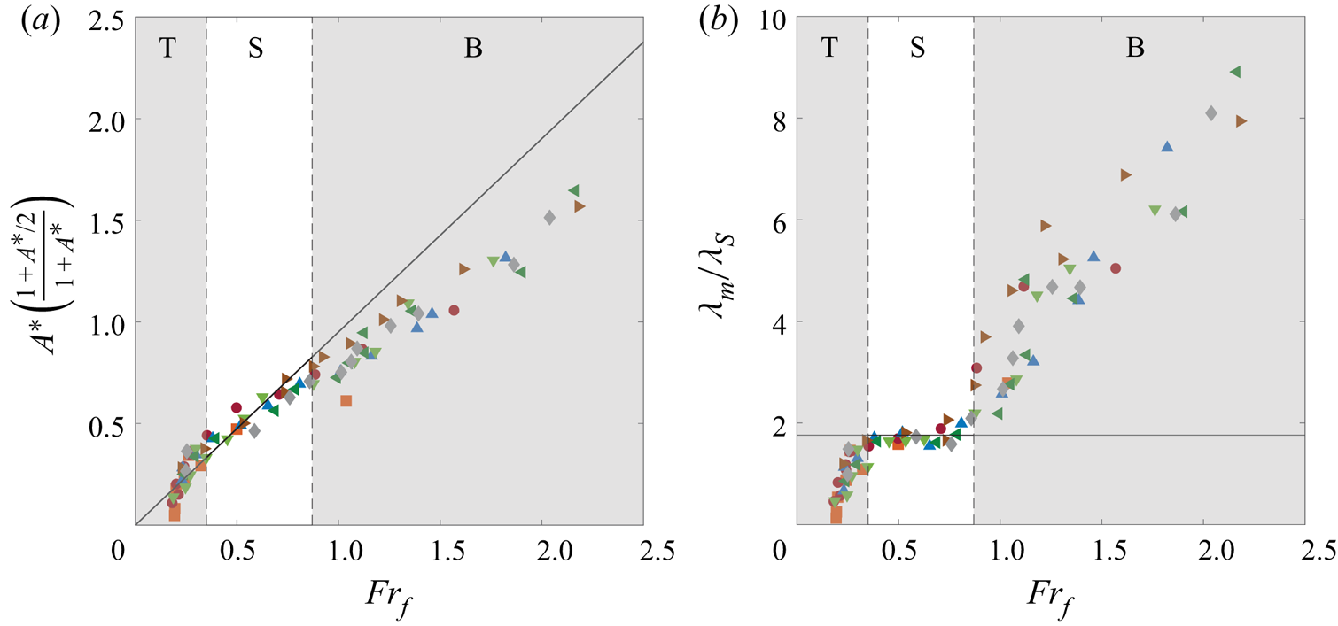
Figure 5(a) shows the rescaled experimental data using the left-hand side of (3.8), with $A_S=A_m$, as a function of ${Fr}_f$. All the experimental data for $0.35 \lesssim {Fr}_f \lesssim 0.87$ collapse well onto a straight line of slope 0.95. Therefore, in the corresponding experiments, the advancing granular front acts as a moving piston with an effective maximal velocity $v_{f_m} = 0.95\ v_p$. This value is a little smaller than one, which may come from the fact that the granular front is not solid but porous and not perfectly vertical. The explicit expression for $A_S/h_0$ as a function of ${Fr}_p$ is obtained as the only positive solution of the second-order equation (3.8):

(3.9)\begin{equation} \frac{A_S}{h_0}={Fr}_p + \sqrt{1+{{Fr}_p}^2}-1. \end{equation}

Figure 5.

(a) Plot of $A^*[(1+A^*/2)/(1+A^*)]$ as a function of ${Fr}_{f}$ for all experiments, with $A^*=A_m/h_0$. The best linear fit (full line) of slope 0.95 for the data corresponding to the solitary wave regime ($0.35 \lesssim {Fr}_{f} \lesssim 0.87$) is also shown. (b) Plot of $\lambda _m/\lambda _S$ as a function of ${Fr}_f$, with the expected plateau value $\lambda _m/\lambda _S=1.76$ (horizontal full line).

The red dashed curve in figure 3(a) corresponds to (3.9) with ${Fr}_p=0.95 {Fr}_f$, and fits well the data for $0.35 \lesssim {Fr}_f \lesssim 0.87$. The exact expression (3.9) can be approximated, using Taylor series, by $A_S/h_0 = {Fr}_p + {{Fr}_p}^2/2$, which differs by less than 4 % up to ${Fr}_p \simeq 0.87$. Note that the expected transition from solitary waves to bores can simply be inferred from the intercept of the approximate law $A_S/h_0 = {Fr}_p + {{Fr}_p}^2/2$ for solitons with the approximate linear law $A_B/h_0 \simeq \sqrt {2} {Fr}_p$ for bores. Considering $A_S = A_B$, by continuity, leads to the critical Froude number ${{Fr}_p}_c = 2(\sqrt {2}-1) \simeq 0.8$ and thus to the critical local Froude number ${{Fr}_f}_c \simeq 2(\sqrt {2}-1)/0.9 \simeq 0.9$. This value corresponds well to the observed transition value of ${{Fr}_f} \simeq 0.87$. Figure 5(b) reports the ratio of the experimental mid-height width $\lambda _m$ relative to the expected length $\lambda _S$ obtained from (3.5). We observe a clear plateau value $\lambda _m/\lambda _S \simeq 1.8$ for $0.35 \lesssim {Fr}_f \lesssim 0.87$, in agreement with the expected value $2 \cosh ^{-1} ( \sqrt {2} ) \simeq 1.76$. This further confirms that the waves observed in regime S correspond to solitary waves. The red dashed curve in figure 3(b), corresponding to the theoretical prediction obtained by combining (3.5b) and (3.9), fits well the data with ${Fr}_p \simeq 0.95 {Fr}_f$, and can be approximated by $2 \cosh ^{-1} ( \sqrt {2} ) \lambda _S/h_0 \simeq 2.03 (1-{Fr}_p/2) {{Fr}_p}^{-1/2}$. In this regime of solitary waves, the relative width $\lambda _m/h_0$ of the wave decreases for increasing ${Fr}_f$, in contrast with the other wave regimes, which makes possible a clear differentiation between them. Hence, while (3.3) and (3.9) give almost the same predictions for the relative amplitude in regime S, as observed in figure 3(a), only the solitary wave model estimates correctly the width of the waves in this regime. From these observations, we conclude that solitary waves are generated for a narrow range of ${Fr}_f$, where the granular collapse acts as a piston wavemaker with variable velocity. Note that these solitary waves are not stable but break for ${Fr}_f \gtrsim 0.60$, corresponding to $A_m/h_0 \gtrsim 0.73$, not far from the critical value 0.78 predicted by Tanaka (Reference Tanaka1986).

3.3. Nonlinear transition waves

For small values of the local Froude number (regime T, with ${Fr}_f \lesssim 0.35$), the waves are characterized by strong unsteadiness (wave flattening after generation), and the presence of a dispersive minor wave train. These waves recall one of those observed by Viroulet et al. (Reference Viroulet, Cébron, Kimmoun and Kharif2013) and correspond to the nonlinear transition waves reported by Fritz et al. (Reference Fritz, Hager and Minor2004). Figure 3 shows that both the amplitude and wavelength of the generated waves vary abruptly at ${Fr}_f \simeq 0.2$. Hence the local Froude number ${Fr}_f$, based on the horizontal velocity of the granular front relative to the velocity of shallow-water waves, is not the relevant parameter in regime T any more, for two reasons. First, the shallow-water condition begins to break down in this regime, as observed in figure 6(a), where the evolution of the dimensionless wave velocity $c/\sqrt {gh_0}$ is reported as a function of ${Fr}_f$. While $c/\sqrt {gh_0} > 1$ when ${Fr}_f \gtrsim 0.35$ for regimes S and B, $c/\sqrt {gh_0}$ decreases abruptly below one when ${Fr}_f \lesssim 0.35$ in regime T. Second, in figure 6(b), where the maximum horizontal extension of the granular front $x_{f_m}$, made dimensionless with the water depth $h_0$, is reported as a function of ${Fr}_f$, we observe that $x_{f_m}/h_0 > 1$ when ${Fr}_f \gtrsim 0.35$ for regimes S and B, whereas $x_{f_m}/h_0 < 1$ when ${Fr}_f \lesssim 0.35$ for regime T. In this last regime, $x_f$ may not be the only relevant parameter encoding the initial perturbation that generates the wave. This could be the vertical extension $y_f$ of the granular collapse just below the water surface or a combination of $y_f$ and $x_f$. Hence, regime T corresponds to a transition from shallow- to deep-water conditions, for which developing a theoretical framework is challenging. Note that, for deep-water conditions, all the parameters characterizing both the granular collapse ($x_f$ and $v_f$) and the generated waves ($A_m$ and $\lambda _m$) are not expected to depend on $h_0$ any more. In that case, wave generation would be related to the Cauchy–Poisson problem, where a surface impulse generates a modulated wave train (Stoker Reference Stoker1957), which may correspond to the fourth regime of weakly nonlinear oscillatory waves mentioned by Fritz et al. (Reference Fritz, Hager and Minor2004).

Figure 6.

(a) Evolution of $c/\sqrt {gh_0}$ with ${Fr}_f$, where the horizontal full line emphasizes a ratio value of one. (b) Plot of $x_{f_m}/h_0$ as a function of ${Fr}_f$, where the horizontal full line shows a ratio value of one.