1 Introduction
A novel structure that has been unearthed in recent years is the super solitary wave (SSW), or the classical ‘supersolitons’, which are the organized extra-nonlinear structures in plasma. They are generally distinguished from their regular counterparts, such as a regular solitary wave (RSW), by the extra wiggles or ‘folds’ in their otherwise bipolar electric field (E-field) data (Hellberg et al. Reference Hellberg, Baluku, Verheest and Kourakis2013), or, more commonly, by the extra subwell in the associated Sagdeev pseudopotential profile (Singh & Lakhina Reference Singh and Lakhina2015). Although Baluku, Hellberg & Verheest (Reference Baluku, Hellberg and Verheest2010) found the first signature of a SSW, it was Dubinov & Kolotkov (Reference Dubinov and Kolotkov2012c ) who coined the term ‘supersoliton’ to describe solutions with amplitudes typically larger than the associated double layer (DL). Initially, due to their extra large amplitudes, a weakly nonlinear analysis (Washimi & Taniuti Reference Washimi and Taniuti1966) was found to be inadequate for their interpretation (Dubinov & Kolotkov Reference Dubinov and Kolotkov2012b ). Later, however weakly nonlinear supersolitons have been reported for a modified form of the Korteweg–de Vries equation (Olivier, Verheest & Maharaj Reference Olivier, Verheest and Maharaj2017; Olivier, Verheest & Hereman Reference Olivier, Verheest and Hereman2018). There is at least one reported piece of evidence where the experimental observation of an ion acoustic wave, travelling in a composite chemical system, has confirmed structures akin to a supersoliton (Dubinov & Kolotkov Reference Dubinov and Kolotkov2012a ). This suggests that the SSW structure is not just a theoretical concept but can also be achieved in an appropriately designed laboratory experiment. The applicability of SSWs has been further enhanced with a recent review (Dubinov & Kolotkov Reference Dubinov and Kolotkov2018) which has suggested SSW-like structures in the E-field data of electrostatic solitary waves (ESWs), observed during satellite expeditions of the Earth’s magnetosphere.
In most of the cases, a SSW is defined by the morphology of the pseudopotential. Alternatively, Dubinov & Kolotkov (Reference Dubinov and Kolotkov2012a ,Reference Dubinov and Kolotkov c ) argued that they appear beyond the separatrix of their phase portraits. This necessarily assumes that a SSW is always associated with a DL solution. The same was validated by others (Hellberg et al. Reference Hellberg, Baluku, Verheest and Kourakis2013; Verheest, Hellberg & Kourakis Reference Verheest, Hellberg and Kourakis2013a ). There was, however, an early indication that SSWs may appear even without a DL (Verheest et al. Reference Verheest, Hellberg and Kourakis2013a ; Verheest, Hellberg & Kourakis Reference Verheest, Hellberg and Kourakis2013b ). Later it was Steffy & Ghosh (Reference Steffy and Ghosh2017) who established that the transition route from a RSW to the corresponding SSW is not unique and need not be associated with a DL. Instead, it may involve other intermediate extra-nonlinear structures, like generalized variable solitary waves (gVSWs) and curves of inflection (CoI). They quantified the associated morphology of the Sagdeev pseudopotential incorporating a derivative analysis and showed that all those aforementioned extra-nonlinear solitary structures, including the SSW, are associated with a fluctuating, or ‘variable’, charge separation within their localized potential profiles. They coined the term variable solitary waves (VSWs) for all those ‘fluctuating’ structures. According to their nomenclature, a SSW is a subset of VSWs and a gVSW is that class of VSWs which excludes more specific type of solutions like a SSW, CoI, or a flat top solitary wave (FTSW) (Varghese & Ghosh Reference Varghese and Ghosh2016; Steffy & Ghosh Reference Steffy and Ghosh2018). Though in the popular literature they are often called ‘supersolitons’, Steffy & Ghosh (Reference Steffy and Ghosh2017) argued that, in the absence of any rigorous analytical formalism, and without any description of its collisional properties, it is more appropriate to call it a ‘super solitary wave’ rather than the ‘supersoliton’.
So far SSWs were mostly found for low frequency waves in an unmagnetized plasma (Hellberg et al. Reference Hellberg, Baluku, Verheest and Kourakis2013; Maharaj et al. Reference Maharaj, Bharuthram, Singh and Lakhina2013; Singh & Lakhina Reference Singh and Lakhina2015). Rufai et al. (Reference Rufai, Bharuthram, Singh and Lakhina2014, Reference Rufai, Bharuthram, Singh and Lakhina2015) were the first to investigate SSWs in a magnetized plasma assuming Cairn’s and Kappa distributions. They further compared their theoretical analyses with the Viking satellite observations in the Earth’s auroral region (Rufai et al. Reference Rufai, Bharuthram, Singh and Lakhina2014, Reference Rufai, Bharuthram, Singh and Lakhina2015, Reference Rufai, Bharuthram, Singh and Lakhina2016; Rufai Reference Rufai2015). They, however, obtained a very spiky, narrow and infinitely deep subwell in the presence of the magnetic field. Though it is assumed to befit the former definition of the SSW, confirming the three local extrema, the associated abruptness appears to defy the proposed derivative analysis of Steffy & Ghosh (Reference Steffy and Ghosh2017). On the contrary, for an unmagnetized plasma, the two subwells of the corresponding pseudopotential are often quite asymmetric but their shapes and sizes are fairly comparable with each other (Maharaj et al. Reference Maharaj, Bharuthram, Singh and Lakhina2013; Verheest et al. Reference Verheest, Hellberg and Kourakis2013b ; Verheest, Hellberg & Kourakis Reference Verheest, Hellberg and Kourakis2013c ; Verheest & Hellberg Reference Verheest and Hellberg2015), leading to the four clear roots of its first derivative (Varghese & Ghosh Reference Varghese and Ghosh2016). For the sake of the convenience, we choose to call them a ‘regular’ SSW. In that sense, the solutions obtained by Rufai and others were not ‘regular’. Verheest & Hellberg (Reference Verheest and Hellberg2017) have pointed out that such a spiky and infinitely deep profile arises due to the singularity and the corresponding ‘blowing up’ of the pseudopotential rather than any possible SSW solution.
Sagdeev pseudopotentials for a magnetized plasma often, indeed, encounter singularities and blowing up of their profiles (Yu Reference Yu1978; Wei & Chen Reference Wei and Chen2005). Previous authors argued that, in spite of the singularity of the pseudopotential, a physical solution may still exist due to its finite and physical potential and they called the corresponding solutions as spiky or cusp solitons. There were reports of such spiky solutions for the lower hybrid (Yu Reference Yu1978; Wei & Chen Reference Wei and Chen2005) and Alfvén solitary waves (Yinhua, Wei & Yu Reference Yinhua, Wei and Yu2000) while Sagdeev pseudopotentials for the electron acoustic wave in a magnetized plasma, too, have indicated a similar type of blowing up and the associated singularities (Ghosh et al. Reference Ghosh, Pickett, Lakhina, Winningham, Lavraud and Décréau2008). The spiky profiles they have obtained for the pseudopotentials appear to be analogous, or related, to that reported by Rufai et al. (Reference Rufai, Bharuthram, Singh and Lakhina2014, Reference Rufai, Bharuthram, Singh and Lakhina2015). However, the association with the singularity in the presence of a magnetic field makes the morphology of the pseudopotential visibly different from that for the unmagnetized plasma and calls for an alternate definition of the SSW for the former.
The analyses presented by Rufai and others (Rufai et al. Reference Rufai, Bharuthram, Singh and Lakhina2014, Reference Rufai, Bharuthram, Singh and Lakhina2015, Reference Rufai, Bharuthram, Singh and Lakhina2016; Rufai Reference Rufai2015), and the rebuttal by Verheest & Hellberg (Reference Verheest and Hellberg2017), throw an open question about the existence of a ‘regular’ SSW solution in a magnetized plasma which will be free from any ambiguity arising due to the singularity. It also calls for an investigation about the effect of the presence of the magnetic field on the SSW and its possible correlations with the singularity. This motivated us to investigate a magnetized SSW in the present work.
It is well known that, when the solar wind crosses the bow shock, ions get energized and eventually becomes hotter than electrons (Treumann & Sagdeev Reference Treumann and Sagdeev2005; Kalra & Kumar Reference Kalra and Kumar2006). In such cases, it was found that an electron acoustic mode can be excited in a plasma. A complete analytical formalism for an arbitrary amplitude electron acoustic solitary wave in a magnetized plasma with energetic ions was elaborated by Buti (Reference Buti1980) where ions were assumed to have Boltzmann distribution and electrons were described by the usual fluid equations. This assumption necessarily ignores the effect of the ions’ inertia which can be justified if the thermal velocity of the species remains higher than the phase velocity of the wave. In the presence of the magnetic field, this can be achievable because of the dependence of the phase velocity on the magnetic field (Buti Reference Buti1980; Mohan & Buti Reference Mohan and Buti1980). Such an assumption, however, would not be valid for an unmagnetized plasma. It was argued that, in a magnetized plasma, electrons are too sluggish whereas the hot and energetic ions are mobile enough to be thermalized due to their much larger Larmor radius (Mohan & Buti Reference Mohan and Buti1980). Following Buti, Ghosh et al. (Reference Ghosh, Pickett, Lakhina, Winningham, Lavraud and Décréau2008) delineated the existence of electron acoustic solitary waves for different regions of the Earth’s magnetosphere. Though they reported both DLs and singularities, there was no indication of SSWs. In order to explore that lacuna, we have decided to adopt their model to investigate electron acoustic SSWs for a magnetized plasma. The problem of the occurrence of the singularity in the Sagdeev pseudopotential profile for a magnetized plasma has itself received a scant attention so far. Besides that, the concept of the SSW is relatively new and requires further understanding. So far there was no reported SSW in a magnetized plasma without any direct association with the singularity. Moreover, there was no high frequency super solitary wave solution reported till date. Our analysis in the present work has revealed a regular electron acoustic super solitary wave for a magnetized plasma. The solution lies in the vicinity of, but sufficiently away from the singularity, ensuring it to be physical. The SSW satisfies all the major criteria of the derivative analysis incorporated by Varghese & Ghosh (Reference Varghese and Ghosh2016) for an unmagnetized plasma and hence can be termed as ‘regular’. To the best of our knowledge, this is also the first theoretical report of a high frequency (electron acoustic) super solitary wave. This enhances the applicability of a SSW to interpret satellite observations like FAST (Ergun et al. Reference Ergun, Carlson, McFadden, Mozer, Delory, Peria, Chaston, Temerin, Roth and Muschietti1998), POLAR (Cattell et al. Reference Cattell, Dombeck, Wygant, Hudson, Mozer, Temerin, Peterson, Kletzing, Russell and Pfaff1999) or CLUSTER multi-spacecraft mission (Pickett et al. Reference Pickett, Chen, Kahler, Santolík, Gurnett, Tsurutani and Balogh2004). An alternative theoretical description has been developed in the present paper to identify a SSW for a magnetized plasma. Our analyses suggest that, in the presence of the magnetic field, a singularity rather than a double layer may play a more vital role in the emergence of a SSW.
The paper is structured as follows. The next section (§ 2) provides the required analytical derivations describing the model (§ 2.1), deducing the parameter set (§ 2.2) and finding the Sagdeev pseudopotential (§ 2.3). Section 3.1 represents the electron acoustic SSW while § 3.2 highlights and categorizes the overall transition processes. The theoretical foundation of the magnetized SSW and its criteria have been presented in § 3.3 on the basis of the denominator of the Sagdeev pseudopotential (§ 3.3.1) and the phase portrait analysis (§ 3.3.2). The concluding remarks are given in § 4 while the appendix A summarizes the detail of all the algebraic terms in § 2.3.
2 The analytical solution
2.1 The model
We have considered a homogeneous, infinite, collisionless and magnetized plasma consisting of four components with two species of hot and energetic ions and warm fluids of beam and bulk electrons. The magnetic field is assumed to be parallel to the
 $z$
direction and the wave is propagating obliquely in the
 $y$
–
 $z$
plane with an angle
 $\unicode[STIX]{x1D703}$
. The wave is governed by the electron dynamics which is assumed to be adiabatic, ensuring an adequately larger time scale compared to the electron plasma frequency of the associated plasma system. On the other hand, ions are assumed to be hotter than the electrons (
 $T_{i}>T_{e}$
) (Kalra & Kumar Reference Kalra and Kumar2006) and obey Boltzmann distributions. The spatio-temporal scale of the ions are determined by their Larmor radius and the inverse of the gyrofrequency which are typically much larger than the wavelength and the time period of the electron acoustic wave. This allows us to consider ions as unmagnetized (Buti Reference Buti1980; Mohan & Buti Reference Mohan and Buti1980). This also makes them freer to get thermalized within the stipulated time period.
For an ion acoustic wave, it is customary to assume electrons as massless, obeying a Boltzmann or some other distribution. An analogous model for an electron acoustic wave is, however, more restricted and is limited to a fairly oblique propagation of the wave in the presence of the ambient magnetic field (Buti Reference Buti1980; Mohan & Buti Reference Mohan and Buti1980). The obliqueness slows down the wave so that, for a chosen parameter set, its phase velocity may eventually become lower than the thermal velocity of the energetic ions. Moreover, in the present case, it is the ions which are providing the pressure for the electron acoustic wave while the electrons, which are assumed as fluids, provide the inertial effect. We assume that the initial perturbation, which eventually leads to the generation of the electron acoustic solitary wave, remains too small to affect the ion dynamics due to its much larger kinetic inertia. It is often customary to consider a simpler analytical model which retains the thermal effect of the energetic ions but ignores inertia (Devanandhan, Singh & Lakhina Reference Devanandhan, Singh and Lakhina2011; Sultana, Kourakis & Hellberg Reference Sultana, Kourakis and Hellberg2012). A more quantitative assessment for this assumption in the present case is given in § 2.2.
The limitation of the Sagdeev pseudopotential technique for a magnetized plasma is that the system is restricted to have not more than one magnetized species. Otherwise, the Sagdeev pseudopotential itself will not be analytically tractable and ought to be found numerically. Verheest (Reference Verheest2009) has further proved analytically that the constrain on the number of magnetized species is an inherent property of the mathematical formalism and is generic for any plasma model. This requires to impose a charge neutrality condition for the model (Devanandhan et al.
Reference Devanandhan, Singh and Lakhina2011; Sultana et al.
Reference Sultana, Kourakis and Hellberg2012). Although an EAW has a fairly high frequency compared to an ion or dust acoustic mode, it is still believed to be slow enough compared to its electron plasma frequency and thus would have enough time to justify the approximation of the charge neutrality. The assumed sluggishness of the electrons is further consistent with their adiabatic condition. The constrains on the net number of the magnetized species further calls for the beam electrons to be highly collimated, moving strictly parallel to the magnetic field without having any cross-component. The single
 $z$
component of its velocity is justified by their extremely small Larmor radius (Das & Bujarbarua Reference Das and Bujarbarua1988; Ghosh et al.
Reference Ghosh, Pickett, Lakhina, Winningham, Lavraud and Décréau2008).
The above model will be applicable for that range of plasma parameters where the thermal velocities of the ions remain larger than the phase velocity of the linear wave. To ascertain our plasma model, we have deduced the linear dispersion relation in the next Section (§ 2.2) and validated the velocities for a selected set of plasma parameters.
2.2 The parameters
The normalized fluid equations governing the four component plasma are
 $$\begin{eqnarray}\displaystyle & \displaystyle \frac{\unicode[STIX]{x2202}N_{eb}}{\unicode[STIX]{x2202}t}+\frac{\unicode[STIX]{x2202}(N_{eb}\boldsymbol{V}_{eb})}{\unicode[STIX]{x2202}z}=0, & \displaystyle\end{eqnarray}$$
 $$\begin{eqnarray}\displaystyle & \displaystyle \frac{\unicode[STIX]{x2202}\boldsymbol{V}_{eb}}{\unicode[STIX]{x2202}t}+\boldsymbol{V}_{eb}\frac{\unicode[STIX]{x2202}\boldsymbol{V}_{eb}}{\unicode[STIX]{x2202}z}=\frac{\unicode[STIX]{x2202}\unicode[STIX]{x1D6F7}}{\unicode[STIX]{x2202}z}-3\unicode[STIX]{x1D70E}_{eb}N_{eb}\frac{\unicode[STIX]{x2202}N_{eb}}{\unicode[STIX]{x2202}z}, & \displaystyle\end{eqnarray}$$
 $$\begin{eqnarray}\displaystyle & \displaystyle \frac{\unicode[STIX]{x2202}N_{es}}{\unicode[STIX]{x2202}t}+\unicode[STIX]{x1D735}\boldsymbol{\cdot }(N_{es}\boldsymbol{V}_{es})=0, & \displaystyle\end{eqnarray}$$
 $$\begin{eqnarray}\displaystyle & \displaystyle \frac{\unicode[STIX]{x2202}\boldsymbol{V}_{es}}{\unicode[STIX]{x2202}t}+(\boldsymbol{V}_{es}\boldsymbol{\cdot }\unicode[STIX]{x1D735})\boldsymbol{V}_{es}=\unicode[STIX]{x1D735}\unicode[STIX]{x1D6F7}-\unicode[STIX]{x1D6FC}_{es}(\boldsymbol{V}_{es}\times \hat{\boldsymbol{b}})-3\unicode[STIX]{x1D70E}_{es}N_{es}\unicode[STIX]{x1D735}N_{es}, & \displaystyle\end{eqnarray}$$
and the ion density
 $$\begin{eqnarray}n_{i}=Z_{1}\unicode[STIX]{x1D707}_{i}\exp \left(\frac{-Z_{1}\unicode[STIX]{x1D6F7}}{Z_{1}^{2}\unicode[STIX]{x1D707}_{i}+Z_{2}^{2}\unicode[STIX]{x1D708}_{i}\unicode[STIX]{x1D6FD}_{i}}\right)+Z_{2}\unicode[STIX]{x1D708}_{i}\exp \left(\frac{-Z_{2}\unicode[STIX]{x1D6FD}_{i}\unicode[STIX]{x1D6F7}}{Z_{1}^{2}\unicode[STIX]{x1D707}_{i}+Z_{2}^{2}\unicode[STIX]{x1D708}_{i}\unicode[STIX]{x1D6FD}_{i}}\right),\end{eqnarray}$$
where the subscripts
 $i$
,
 $eb$
(
 $es$
) and
 $ic$
(
 $ih$
) represent ions, beam (bulk) electrons and cooler (hotter) ions respectively,
 $N_{eb(es)}\,(=n_{eb(es)}/\unicode[STIX]{x1D70C}_{eb(es)})$
is the ratio of beam (bulk) electron densities to their respective ambient densities,
 $\unicode[STIX]{x1D70C}_{eb}$
(
 $\unicode[STIX]{x1D70C}_{es}$
) and
 $\unicode[STIX]{x1D707}_{i}$
(
 $\unicode[STIX]{x1D708}_{i}$
) being the ambient number densities of beam (bulk) electrons and cooler (hotter) ions respectively, and
 $Z_{1}$
,
 $Z_{2}$
are the respective charge multiplicities for the ions. All the plasma particle temperatures are normalized by the effective ion temperature
 $T_{\text{iff}}\,(=T_{ic}T_{ih}/(Z_{1}^{2}\unicode[STIX]{x1D707}_{i}T_{ih}+Z_{2}^{2}\unicode[STIX]{x1D708}_{i}T_{ic}))$
,
 $\unicode[STIX]{x1D70E}_{eb(es)}\,(=T_{eb(es)}/T_{\text{iff}})$
are the ratio of beam (bulk) electron temperatures to the effective ion temperature, and
 $\unicode[STIX]{x1D6FD}_{i}\,(=T_{ic}/T_{ih})$
is the cooler to hotter ion temperature ratio,
 $T_{ic}$
(
 $T_{ih}$
) and
 $T_{eb}$
(
 $T_{es}$
) being the respective particle temperatures for cooler (hotter) ions and beam (bulk) electrons. The initial normalized velocity of the beam electrons is
 $U_{eb}$
, and
 $\unicode[STIX]{x1D6FC}_{es}\,(=\unicode[STIX]{x1D6FA}_{ce}/\unicode[STIX]{x1D714}_{pe})$
denotes the ratio of the electron cyclotron (
 $\unicode[STIX]{x1D6FA}_{ce}$
) to the electron plasma frequency (
 $\unicode[STIX]{x1D714}_{pe}$
).
According to our normalization scheme, we have normalized all the number densities by the equilibrium plasma density
 $n_{0}$
, time and length by the inverse of the electron plasma frequency
 $\unicode[STIX]{x1D714}_{pe}^{-1}\,(=\sqrt{m_{e}/4\unicode[STIX]{x1D70B}n_{0}e^{2}})$
and the effective ion Debye length
 $\unicode[STIX]{x1D706}_{\text{diff}}\,(=\sqrt{T_{\text{iff}}/4\unicode[STIX]{x1D70B}n_{0}e^{2}})$
respectively, all the velocities including the beam velocity
 $U_{eb}$
by the effective electron acoustic speed
 $C_{\text{iff}}\,(=\sqrt{T_{\text{iff}}/m_{e}})$
, and potential by
 $T_{\text{iff}}/e$
. For our convenience, we have defined
 $M_{\text{eff}}$
as the effective Mach number of the wave which is the normalized wave velocity, normalized by
 $C_{\text{iff}}$
. This is different from the original, or true Mach number of the wave which is deduced from the actual linear electron acoustic speed obtained from the corresponding dispersion relation (Dubinov Reference Dubinov2009). All the partial pressures
 $P_{ej}$
for electrons are normalized by the electron equilibrium pressure
 $P_{0}\,=\,n_{0}T_{e}$
where
 $T_{e}\,(=\unicode[STIX]{x1D70C}_{eb}T_{eb}+\unicode[STIX]{x1D70C}_{es}T_{es})$
is the equilibrium temperature for electrons,
 $j$
being
 $b$
,
 $s$
, respectively for the beam and bulk electrons, and the magnetic field is normalized by the ambient magnetic field
 $B_{0}$
,
 $\hat{\boldsymbol{b}}$
being the unit vector along the magnetic field.
The equations governing the linear electrostatic wave, viz., equations (2.1)–(2.5) are further coupled with the Poisson’s equation
 $$\begin{eqnarray}\unicode[STIX]{x1D6FB}^{2}\unicode[STIX]{x1D6F7}=n_{e}-n_{i}.\end{eqnarray}$$
To find the dispersion relation, we have linearized equations (2.1)–(2.6) and applied the following boundary conditions
 $$\begin{eqnarray}\text{at}\quad |\boldsymbol{r}|\rightarrow \infty ,\quad \unicode[STIX]{x1D6F7}\rightarrow 0,\quad V_{eb}\rightarrow U_{eb},\quad V_{es}\rightarrow 0,\end{eqnarray}$$
 $$\begin{eqnarray}n_{ej}\rightarrow \unicode[STIX]{x1D70C}_{ej},\quad N_{ej}\rightarrow 1,\quad \mathop{\sum }_{j=b,s}n_{ej}\rightarrow 1\quad \text{and}\quad P_{ej}\rightarrow \unicode[STIX]{x1D70C}_{ej}\frac{T_{ej}}{T_{e}}.\end{eqnarray}$$
where
 $\boldsymbol{r}=\boldsymbol{k}_{y}y+\boldsymbol{k}_{z}z$
is the corresponding position vector,
 $\boldsymbol{k}_{y}$
,
 $\boldsymbol{k}_{z}$
being the direction cosines along the
 $y$
and
 $z$
directions respectively.
After some rearrangement, the non-normalized linear dispersion relation is given as,
 $$\begin{eqnarray}1-\frac{\unicode[STIX]{x1D714}_{ps}^{2}(\unicode[STIX]{x1D714}^{2}-\unicode[STIX]{x1D6FA}_{ce}^{2}\text{cos}^{2}\unicode[STIX]{x1D703})}{\unicode[STIX]{x1D714}^{2}(\unicode[STIX]{x1D714}^{2}-\unicode[STIX]{x1D6FA}_{ce}^{2})-3V_{ths}^{2}k^{2}(\unicode[STIX]{x1D714}^{2}-\unicode[STIX]{x1D6FA}_{ce}^{2}\text{cos}^{2}\unicode[STIX]{x1D703})}-\frac{\unicode[STIX]{x1D714}_{pb}^{2}\text{cos}^{2}\unicode[STIX]{x1D703}}{(\unicode[STIX]{x1D714}-kU_{eb}\text{cos}\,\unicode[STIX]{x1D703})^{2}-3V_{thb}^{2}k^{2}}+\frac{e^{2}I}{k^{2}\unicode[STIX]{x1D716}_{0}}=0,\end{eqnarray}$$
where
 $$\begin{eqnarray}I=\frac{Z_{1}^{2}n_{ic0}}{T_{ic}}+\frac{Z_{2}^{2}n_{ih0}}{T_{ih}},\end{eqnarray}$$
and
 $\unicode[STIX]{x1D714}_{pj}$
and
 $V_{thj}$
are the plasma frequency and the thermal velocity of the beam and bulk electrons, with
 $j=eb,es$
respectively. The equation (2.9) has six roots which defines the corresponding linear modes of the wave. There are two negative roots which are non-physical and one root is for a pure electron cyclotron mode. The remaining three acoustic modes will determine the feasibility of our model and the required parameter space.
To determine the parameter range, we followed Ghosh et al. (Reference Ghosh, Pickett, Lakhina, Winningham, Lavraud and Décréau2008) who had chosen a cusp event on 19 February 2002, 2324:11 UT (Universal Time). The location of the spacecraft was at
 $11R_{E}$
(radius of Earth),
 $60\unicode[STIX]{x1D706}_{M}$
(geomagnetic latitude) and 14 h MLT (magnetic local time), and the range of angles of the electric antenna to the magnetic field for this event was
 $35^{\circ }$
–
 $65^{\circ }$
. Accordingly, we have chosen the obliqueness
 $\unicode[STIX]{x1D703}=60^{\circ }$
for our model. The recorded ambient magnetic field was
 $15~\text{nT}$
, the plasma equilibrium density was
 $9.45~\text{cm}^{-3}$
and the electron temperature was
 ${\approx}33.2~\text{eV}$
. The first two parameters give a cyclotron frequency
 $\unicode[STIX]{x1D6FA}_{ce}=414.022~\text{Hz}$
and a plasma frequency
 $\unicode[STIX]{x1D714}_{pe}=27.601~\text{kHz}$
respectively, from which we have deduced
 $\unicode[STIX]{x1D6FC}_{es}=0.015$
. Since the cusp has a significant presence of
 $O^{+}$
, we have assumed that the plasma contains both
 $H^{+}$
and
 $O^{+}$
, the latter being the cooler component with
 $\unicode[STIX]{x1D707}_{i}=0.4$
. The recorded ion temperatures were ranged from
 $100~\text{eV}$
to a few keVs. For our theoretical convenience, we have chosen a hotter ion temperature
 $T_{ih}=6000~\text{eV}$
while for the cooler one
 $T_{ic}=150~\text{eV}$
, giving rise to a
 $\unicode[STIX]{x1D6FD}_{i}=1/40$
. According to our normalization scheme, these give rise to
 $T_{\text{iff}}=361.4458~\text{eV}$
,
 $C_{\text{iff}}=7.9732\times 10^{3}~\text{km}~\text{s}^{-1}$
and
 $\unicode[STIX]{x1D706}_{\text{diff}}=45.948~\text{m}$
which determine the scale of our plasma model. Following CLUSTER observations, we have assumed electron temperatures
 $T_{eb}$
 $(T_{es})=9.0361~\text{eV}$
 $(12.0482~\text{eV})$
, giving rise to
 $\unicode[STIX]{x1D70E}_{eb}=1/40$
 $(\unicode[STIX]{x1D70E}_{es}=1/30)$
respectively. For the beam electrons, we have chosen a beam electron speed of
 $u_{eb}=3.9865\times 10^{3}~\text{km}~\text{s}^{-1}$
, giving rise to the corresponding normalized
 $U_{eb}=0.5$
. In the absence of any data for two electron populations, we have chosen bulk electrons to be 50 % of the total population, i.e.
 $\unicode[STIX]{x1D70C}_{es}=0.5$
.
For the above mentioned set of plasma parameters, we have selected three values of
 $k$
, viz., low, medium and high, and deduced the corresponding three roots of
 $\unicode[STIX]{x1D714}$
for the acoustic modes of the waves (2.9). We have further estimated the associated phase velocity
 $V_{p}=\unicode[STIX]{x1D714}/k$
, and the thermal velocities of the ions, viz.,
 $V_{tij}=\sqrt{T_{ij}/m_{ij}}$
, where
 $j=c,h$
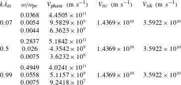
being the cooler and hotter ions respectively. In table 1, we have enlisted the plasma modes, the corresponding non-normalized phase velocities, and the non-normalized thermal velocities of the ions. It reveals that, for an wide range of
 $k$
, and for two acoustic modes out of three, both of the ion’s thermal velocities remain consistently higher than the associated wave phase velocity. This means that, for those modes, and for that selected parameter space, ions can be assumed as Boltzmann. This further supports our model for the present analysis.
Comparison between the thermal and phase velocity for the chosen parameters.

2.3 Sagdeev pseudopotential
As mentioned earlier (§ 2.1), to deduce a nonlinear wave solution, we need to incorporate the charge neutrality condition in the place of the Poisson’s equation (2.6)
 $$\begin{eqnarray}n_{i}=Z_{1}n_{ic}+Z_{2}n_{ih}=n_{eb}+n_{es}.\end{eqnarray}$$
Further, to solve the set of nonlinear partial differential equations, viz., equations (2.1)–(2.5), a stationary state solution is assumed,
 $$\begin{eqnarray}\unicode[STIX]{x1D702}=k_{y}y+k_{z}z-M_{\text{eff}}t,\end{eqnarray}$$
where
 $k_{y}$
,
 $k_{z}$
and
 $M_{\text{eff}}$
are defined in § 2.2, and
 $\unicode[STIX]{x1D702}$
is the generalized coordinate. Solving (2.1)–(2.5), along with (2.11) we obtain
 $$\begin{eqnarray}\frac{\text{d}}{\text{d}\unicode[STIX]{x1D702}}\left[\frac{1}{2}\frac{1}{N_{es}}\frac{\text{d}^{2}}{\text{d}\unicode[STIX]{x1D702}^{2}}\left\{\left(\frac{M_{\text{eff}}}{N_{es}}\right)^{2}+3\unicode[STIX]{x1D70E}_{es}N_{es}^{2}-2\unicode[STIX]{x1D6F7}\right\}+\unicode[STIX]{x1D6FC}_{es}^{2}\left\{\frac{1}{N_{es}}+\frac{k_{z}^{2}}{M_{\text{eff}}^{2}}(\unicode[STIX]{x1D70E}_{es}N_{es}^{3}-\widetilde{N}_{es})\right\}\right]=0,\end{eqnarray}$$
where
 $$\begin{eqnarray}\widetilde{N}_{es}=\int N_{es}\,\text{d}\unicode[STIX]{x1D6F7}.\end{eqnarray}$$
Integrating (2.13) and using boundary conditions ((2.7), (2.8)), we obtain the well-known form for the resultant equation
 $$\begin{eqnarray}\frac{\text{d}^{2}f}{\text{d}\unicode[STIX]{x1D702}^{2}}+\unicode[STIX]{x1D6FC}_{es}^{2}g=0,\end{eqnarray}$$
where
 $$\begin{eqnarray}f=\frac{1}{2}\left(\frac{M_{\text{eff}}^{2}}{N_{es}^{2}}+3\unicode[STIX]{x1D70E}_{es}N_{es}^{2}\right)-\unicode[STIX]{x1D6F7},\end{eqnarray}$$
and
 $$\begin{eqnarray}g=1+\frac{k_{z}^{2}}{M_{\text{eff}}^{2}}(\unicode[STIX]{x1D70E}_{es}N_{es}^{4}-N_{es}\widetilde{N}_{es})-N_{es}\left(1+\frac{k_{z}^{2}}{M_{\text{eff}}^{2}}(\unicode[STIX]{x1D70E}_{es}-\unicode[STIX]{x1D6FF})\right).\end{eqnarray}$$
Integrating (2.15) once again, and after some algebra, leads to the familiar energy condition,
 $$\begin{eqnarray}\frac{1}{2}\left(\frac{\text{d}\unicode[STIX]{x1D6F7}}{\text{d}\unicode[STIX]{x1D702}}\right)^{2}+\unicode[STIX]{x1D6F9}(\unicode[STIX]{x1D6F7})=0,\end{eqnarray}$$
where
 $\unicode[STIX]{x1D6F9}(\unicode[STIX]{x1D6F7})$
is the Sagdeev pseudopotential given by
 $$\begin{eqnarray}\unicode[STIX]{x1D6F9}(\unicode[STIX]{x1D6F7})=\frac{\unicode[STIX]{x1D6FC}_{es}^{2}L_{e}}{F^{2}},\end{eqnarray}$$
 $L_{e}$
,
 $F$
being algebraic functions of
 $\unicode[STIX]{x1D6F7}$
,
 $N_{es}$
,
 $\text{d}N_{es}/\text{d}\unicode[STIX]{x1D6F7}$
and other parameters. The details of all the algebraic terms in (2.19) are given in appendix A.
The Sagdeev pseudopotential ensures a solitary wave solution, provided the following conditions are satisfied.
 $$\begin{eqnarray}\displaystyle \unicode[STIX]{x1D6F9}(\unicode[STIX]{x1D6F7})|_{\unicode[STIX]{x1D6F7}=0}=\frac{\unicode[STIX]{x2202}\unicode[STIX]{x1D6F9}(\unicode[STIX]{x1D6F7})}{\unicode[STIX]{x2202}\unicode[STIX]{x1D6F7}}\bigg|_{\unicode[STIX]{x1D6F7}=0}=0\quad \text{and}\quad \frac{\unicode[STIX]{x2202}^{2}\unicode[STIX]{x1D6F9}(\unicode[STIX]{x1D6F7})}{\unicode[STIX]{x2202}\unicode[STIX]{x1D6F7}^{2}}\bigg|_{\unicode[STIX]{x1D6F7}=0}<0;\end{eqnarray}$$
 $$\begin{eqnarray}\displaystyle \unicode[STIX]{x1D6F9}(\unicode[STIX]{x1D6F7})<0\quad \text{for }\left\{\begin{array}{@{}l@{}}0<\unicode[STIX]{x1D6F7}<\unicode[STIX]{x1D6F7}_{0}\quad \text{when }\unicode[STIX]{x1D6F7}_{0}>0\quad \\ \unicode[STIX]{x1D6F7}_{0}<\unicode[STIX]{x1D6F7}<0\quad \text{when }\unicode[STIX]{x1D6F7}_{0}<0,\quad \end{array}\right.\quad \unicode[STIX]{x1D6F9}(\unicode[STIX]{x1D6F7}_{0})=0\quad \text{and}\quad \frac{\unicode[STIX]{x2202}\unicode[STIX]{x1D6F9}}{\unicode[STIX]{x2202}\unicode[STIX]{x1D6F7}}\bigg|_{\unicode[STIX]{x1D6F7}=\unicode[STIX]{x1D6F7}_{0}}\neq 0,\end{eqnarray}$$
 $\unicode[STIX]{x1D6F7}_{0}$
is the amplitude of the solitary wave.
3 The nonlinear wave
In § 2.2, we have deduced a set of plasma parameters which shows that, for two out of three acoustic modes, thermal velocities for both the ion species are greater than the phase velocity of the linear wave. This is consistent with our assumption that the ions are following Boltzmann distribution. For our nonlinear wave solutions, we have adopted the model of Ghosh et al. (Reference Ghosh, Pickett, Lakhina, Winningham, Lavraud and Décréau2008) and delineated it with the deduced set of normalized plasma parameters (§ 2.2). Throughout our analysis we have assumed single charge multiplicities for both the ions, i.e.
 $Z_{1}=Z_{2}=1$
. We have also assumed a weak magnetization (i.e.
 $\unicode[STIX]{x1D6FA}_{ce}<\unicode[STIX]{x1D714}_{pe}$
) by selecting
 $\unicode[STIX]{x1D6FC}_{es}=0.015$
, and have chosen a beam velocity
 $U_{eb}=0.5$
, as mentioned earlier. To find the extra-nonlinear solution, we have chosen the ambient number density of the cooler ion
 $\unicode[STIX]{x1D707}_{i}=0.4$
and the cooler to hotter ion temperature ratio
 $\unicode[STIX]{x1D6FD}_{i}=1/40$
. Following our linear analysis, we have assumed equal concentrations for the bulk and beam electrons, i.e.
 $\unicode[STIX]{x1D70C}_{es}=\unicode[STIX]{x1D70C}_{eb}=0.5$
while both of them assumed to be sufficiently cooler than the ions, typically
 $\unicode[STIX]{x1D70E}_{eb,es}<1/10$
to eradicate any wave–particle interaction. This further validates our assumption of the fluid model. For the present case, we have assumed the beam electrons to be slightly cooler (i.e.
 $\unicode[STIX]{x1D70E}_{eb}=1/40$
) compared to the bulk (
 $\unicode[STIX]{x1D70E}_{es}=1/30$
). We have chosen an obliqueness of
 $\unicode[STIX]{x1D703}=60^{\circ }$
and varied the effective Mach number
 $M_{\text{eff}}$
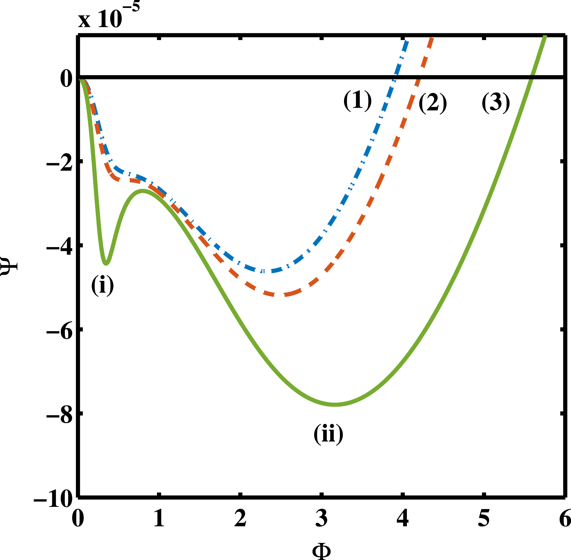
to delineate the corresponding Sagdeev pseudopotentials. Figure 1 shows solitary wave solutions for three different effective Mach numbers, namely
 $M_{\text{eff}}=0.77$
,
 $0.77846132$
and
 $0.81$
, marked as curves (1)–(3) respectively. The curves satisfy the recurrence condition in (2.20d
), which implies solitary wave solutions. For our chosen set of parameters, the existence domain initiates at
 $M_{\text{eff}}=0.7$
and terminates at
 $M_{\text{eff}}=0.84$
. For a larger value of
 $M_{\text{eff}}$
, (e.g.
 $M_{\text{eff}}>0.84$
), the pseudopotential ‘blows up’, indicating a possible case of singularity which we choose to omit as non-physical.
Sagdeev pseudopotential profiles; curves (1) gVSW, (2) n-CoI (see § 3.2) and (3) SSW.

3.1 The super solitary wave (curve (3))
A super solitary wave is primarily defined by the extra subwell of the Sagdeev pseudopotential, or by its four extrema, i.e. the three local extrema along with that at
 $\unicode[STIX]{x1D6F7}=0$
. Curve (3) clearly satisfies the criteria and hence may be considered as a SSW. We found that the two subwells, marked as (i) and (ii) in figure 1, differ markedly by their shapes and sizes. The first subwell, marked as (i), appears at a low potential and is considerably narrow and spiky. For our convenience, we call it the auxiliary subwell while the subwell at the larger potential, marked (ii), is considerably wide and smooth and we call it the main subwell.
The spiky shape of the auxiliary subwell raises the concern whether the solution is an artefact of the possible singularity. On the other hand, in spite of the spiky structure, the depth and width of the auxiliary subwell remain fairly comparable to those of the main one. In § 1 we have argued that, in such cases, the solution is worth considering as a ‘regular’ SSW. Remembering the ambiguity about the previously observed solutions in a magnetized plasma (Rufai et al.
Reference Rufai, Bharuthram, Singh and Lakhina2014, Reference Rufai, Bharuthram, Singh and Lakhina2015, Reference Rufai, Bharuthram, Singh and Lakhina2016; Rufai Reference Rufai2015; Verheest & Hellberg Reference Verheest and Hellberg2017), we have thus incorporated an
 $F$
-analysis for the corresponding pseudopotential where we have plotted the variation of the denominator
 $F$
(equations (2.19) and (A 6)) with
 $\unicode[STIX]{x1D6F7}$
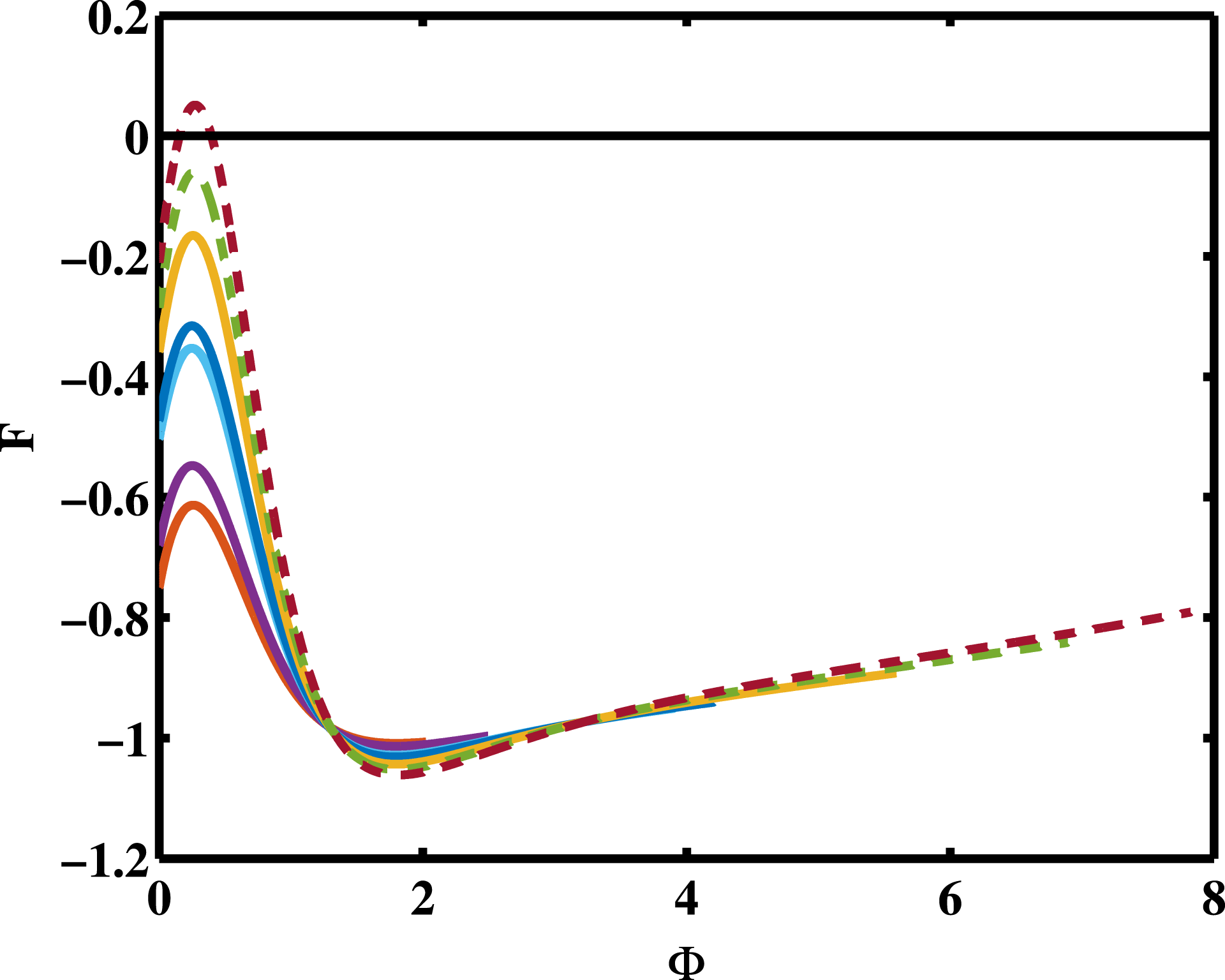
in figure 2. The solid curves are associated with the effective Mach number
 $0.7\leqslant M_{\text{eff}}\leqslant 0.81$
, including the curves (1)–(3) of figure 1, and the dashed curves show the corresponding profiles for two larger values of
 $M_{\text{eff}}$
, viz.,
 $M_{\text{eff}}=0.83$
and
 $0.85$
respectively. Typically, all the profiles show an initial increase, followed by a sharp drop in
 $F$
, resulting in a maximum at the low potential. After a substantial drop in the profile, there is another slow but regular increase in
 $F$
, giving rise to a minimum at a moderate value of
 $\unicode[STIX]{x1D6F7}$
. Compared to the maximum, which looks quite spiky, the minimum appears to be much defused. A comparison between figures 1 and 2 clearly reveals that the corresponding maximum of the
 $F$
profile in figure 2 trivially coincides with the auxiliary subwell of curve (3) in figure 1. However, throughout its variation,
 $F$
remains non-zero (
 $F\neq 0$
) eliminating any possibility of the singularity. The
 $F$
-analysis thus confirms that the solution associated with curve (3) is indeed a physical one and is not an artefact. This also confirms that curve (3) represents a regular electron acoustic SSW in a magnetized plasma.
A closer inspection of figure 2 reveals that, with increasing
 $M_{\text{eff}}$
, the value of
 $F$
at the maximum (
 $=F_{\text{max}}$
) increases, approaching the zero axis, (i.e.
 $F_{\text{max}}\rightarrow 0$
), while the corresponding minimum tends to a lower value. For
 $M_{\text{eff}}=0.83$
(dashed line),
 $|F_{\text{max}}|$
tends to be sufficiently small, initiating a ‘blowing up’ of the pseudopotential which gives rise to an exceptionally deep and spiky auxiliary subwell. Though the morphology of such pseudopotential differs significantly from that of a regular SSW, the solution still remains acceptable and physical without any singularity (
 $F\neq 0$
). As
 $M_{\text{eff}}$
increases further,
 $F_{\text{max}}$
turns positive for
 $M_{\text{eff}}=0.85$
ensuring a zero value for
 $F$
in between. As
 $F$
becomes zero,
 $\unicode[STIX]{x1D6F9}$
becomes non-physical for that particular value of
 $\unicode[STIX]{x1D6F7}$
. This further validates the imminence of the singularity.
 $F$
variation for the chosen parametric regime.

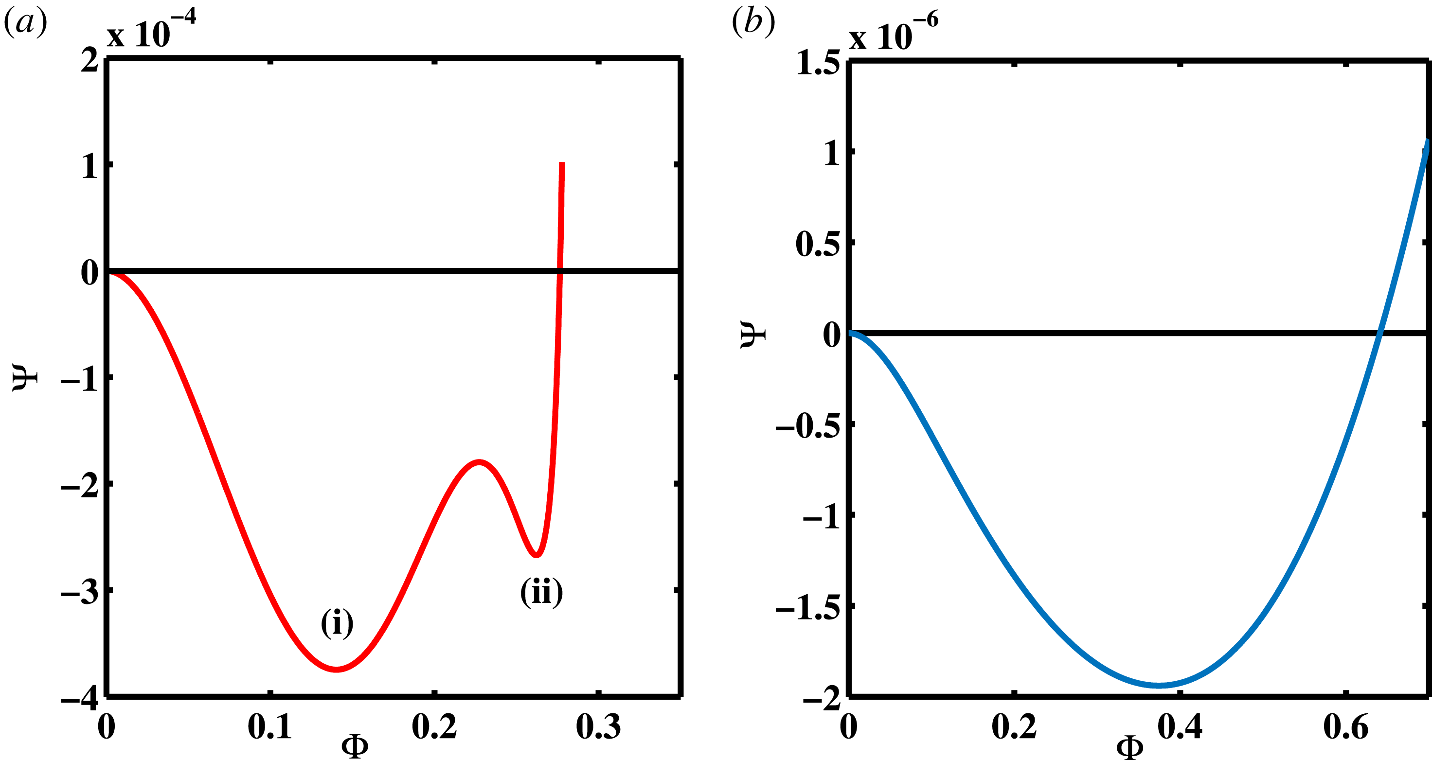
Sagdeev pseudopotential; (a) for SSW of unmagnetized plasma and (b) for RSW of magnetized plasma.

From the above analysis we may conclude that a regular SSW is supported in a magnetized plasma as well. For the present case, the SSW has occurred in the vicinity of the singularity and, apparently, caused by a fluctuating
 $F$
which shows a steep increase, followed by a maximum, at a low potential. Previously Varghese & Ghosh (Reference Varghese and Ghosh2016) have shown that, for an unmagnetized plasma, the SSW is associated with the overall fluctuation in the charge separation. Since we have assumed a charge neutrality condition, such an inference is not applicable for the present case. This implies that the factors governing the emergence of the SSW for a magnetized and unmagnetized cases may well differ to a good extent.
To facilitate a more rigorous comparison between the two, we have adopted the model of Varghese & Ghosh (Reference Varghese and Ghosh2016) for an unmagnetized plasma and plotted the corresponding Sagdeev pseudopotential for a compressive (positive amplitude) ion acoustic SSW in figure 3(a). The particular analytical form of the Sagdeev pseudopotential has been obtained and explained in Varghese & Ghosh (Reference Varghese and Ghosh2016). The model consists of a four component plasma comprising two temperature electrons having Boltzmann distributions and two species of adiabatically warm ions (viz.,
 $H^{+}$
and
 $O^{+}$
) with the lighter to the heavier ion mass ratio
 $Q=1/16$
. We have chosen a convenient set of parameters to support the SSW solution where the cooler to hotter electron temperature ratio
 $\unicode[STIX]{x1D6FD}_{e}=0.048$
, the ambient density of the cooler electrons
 $\unicode[STIX]{x1D707}_{e}=0.00109$
, that for the lighter ions
 $\unicode[STIX]{x1D70C}_{il}=0.9$
, and the normalized ion temperatures for both the species is
 $\unicode[STIX]{x1D70E}_{i}=0.033$
,
 $M_{\text{eff}}=1.06$
being the corresponding effective Mach number. To complement our investigations, we have also chosen a different set of parameters for our own model describing a magnetized plasma and plotted the corresponding Sagdeev pseudopotential in figure 3(b). It reveals a positive amplitude (rarefactive) electron acoustic RSW moving with
 $M_{\text{eff}}=0.75$
. To obtain the required solution (figure 3
b), we have chosen a comparatively cooler bulk electrons where both the beam and the bulk electrons are assumed to have an equal temperature, i.e.
 $\unicode[STIX]{x1D70E}_{es}=\unicode[STIX]{x1D70E}_{eb}=1/40$
, ambient density of cooler ions are considered to be
 $\unicode[STIX]{x1D707}_{i}=0.2$
, ratio of electron cyclotron to plasma frequency is
 $\unicode[STIX]{x1D6FC}_{es}=0.5$
and all other parameters remain the same as figure 1.
Following figure 1, we have marked the two subwells as (i) and (ii) in figure 3(a), depending on their respective positions starting from
 $\unicode[STIX]{x1D6F7}=0$
towards the maximum amplitude. This shows that the subwell (i) in figure 3(a) is much wider and deeper and is eventually the main subwell with subwell (ii) the auxiliary one. A comparison between these two figures, viz., figures 1 and 3(a) readily reveals a lateral inversion of the mutual positions of the main and the auxiliary subwells. According to our prior definition, the main subwell is the wider and the smoother part of the two, accompanied by the auxiliary one where the latter causes the characteristic wiggles of the SSW. In the absence of the magnetic field, the main subwell (subwell (i) in figure 3
a) occurs at the lower potential which is followed by a shorter auxiliary subwell (subwell (ii)) near the maximum amplitude. In the presence of the magnetic field (figure 1), the trend becomes just the opposite. It is the low potential subwell (i) which turns to be the narrow and spiky auxiliary subwell, followed by a smoother and wider main subwell (subwell (ii)) for a larger potential. While most of the previous observations of unmagnetized SSWs have shown the former trend, Dubinov, Kolotkov & Sazonkin (Reference Dubinov, Kolotkov and Sazonkin2012) have reported a Sagdeev pseudopotential with an auxiliary subwell near
 $\unicode[STIX]{x1D6F7}=0$
for an Alfvén wave which, once again, indicates the possible influence of the magnetic field.
We note that all the above profiles, viz., figures 1 and 3, depict positive polarity solutions. However, the positive polarity solutions for the electron acoustic solitary waves in figures 1 and 3(b) indicate rarefaction of electrons (potential well) while for the ion acoustic wave and unmagnetized plasma (figure 3 a), it becomes a potential hill due to the compression of ions. It is well known that the amplitude of a compressive ion acoustic solitary wave is limited by its energy condition (Ghosh & Iyengar Reference Ghosh and Iyengar1997; Varghese & Ghosh Reference Varghese and Ghosh2016; Steffy & Ghosh Reference Steffy and Ghosh2017). On the other hand, being a potential well, the amplitude of the positive polarity electron acoustic solitary wave (viz., figures 1 and 3 b) has no such bound. An analogous situation arises for a rarefactive (negative amplitude) ion acoustic solitary wave (Ghosh, Ghosh & Iyengar Reference Ghosh, Ghosh and Iyengar1996; Ghosh & Sekar Iyengar Reference Ghosh and Sekar Iyengar2002). Most of the rarefactive ion or dust acoustic SSWs in the unmagnetized plasma have reported auxiliary subwells at higher potentials. The one exception is Dubinov & Kolotkov (Reference Dubinov and Kolotkov2012a ) who have reported a low potential auxiliary subwell for a rarefactive ion acoustic SSW in a complex chemical system. This suggests that, even in the absence of a magnetic field, a low potential auxiliary subwell may arise for a rarefactive solution. Previously Steffy & Ghosh (Reference Steffy and Ghosh2017) have suggested that the wiggle of the potential profile, associated with the auxiliary subwell for the SSW, shifts to the lower potential with increasing amplitude or nonlinearity. We may here conjecture that the presence of the magnetic field contributes to an extra-nonlinearity which shifts the auxiliary subwell to a lower potential. Alternatively, the rarefaction of an oscillating species may also play a significant role in generating the wiggle, or the associated auxiliary subwell, near the smaller potential causing the observed inversion of its position. A more quantitative understanding of this process is beyond the scope of the present work and may be communicated elsewhere.
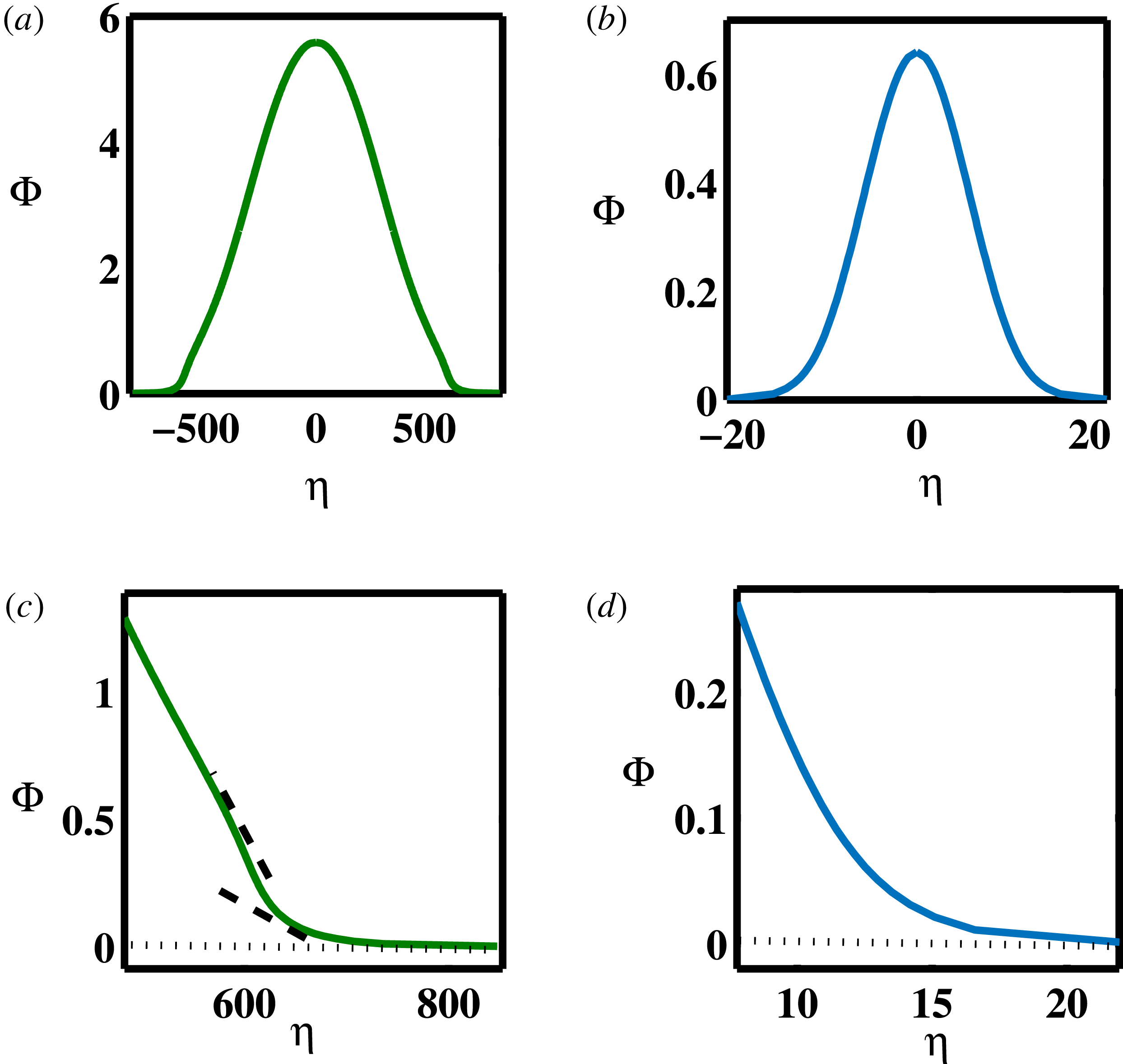
The potential profile of (a) SSW and (b) RSW; the enlarged low potential part of (c) SSW and (d) RSW.

The implication of the low potential auxiliary subwell for the magnetized plasma becomes clearer in figure 4(a) where we have plotted the potential profile for curve (3) of figure 1, obtained numerically by integrating (2.18) in terms of the generalized coordinate
 $\unicode[STIX]{x1D702}$
. For the sake of the comparison, we have also plotted the potential profile of the RSW in figure 4(b), corresponding to the pseudopotential shown in figure 3(b). At first glance, the two potential profiles, viz., figures 4(a) and 4(b), look alike, both showing the usual bell shaped profiles. A closer inspection, however, reveals that the profile of the SSW appears to end abruptly near the zero axis (figure 4
a) while that for the RSW (figure 4
b) varies smoothly. For a better view, we have enlarged the corresponding low potential variation of the two profiles, viz., figures 4(a) and 4(b), in figures 4(c) and 4(d) respectively. These highlights show that the RSW profile (figure 4
d) approaches the zero axis asymptotically, remaining concave downward throughout its variation, whereas there is an abrupt change of the slope for the SSW in figure 4(c) before
 $\unicode[STIX]{x1D6F7}$
approaches zero. The change in the slope is further marked by the two dashed lines in figure 4(c). This also makes the curve slightly ‘convex’ (concave downwards) between
 $590<\unicode[STIX]{x1D702}<610$
which is known to be the hallmark of a SSW. The low potential auxiliary subwell of the Sagdeev pseudopotential produces a wiggle near the base of the corresponding potential profile due to the sudden change in its slope, or the ‘generalized electric field’ (2.18). For an usual SSW reported so far for an unmagnetized plasma, however, the wiggle in the potential profile generally appears at its ‘knee’ rather than the base of the profile.
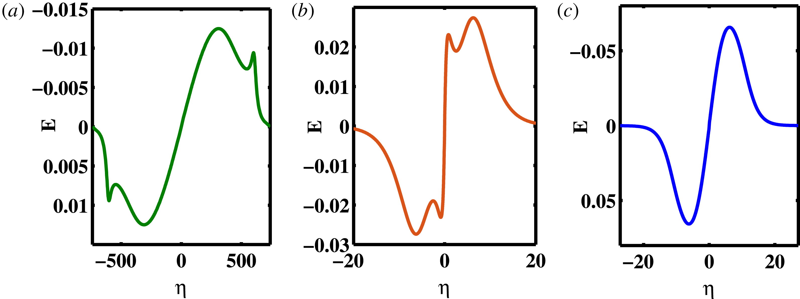
The swapping of the auxiliary subwell as reported in figures 1 and 3(a) not only influences the position of the wiggle in the potential profile (figure 4 a) but also causes their lateral inversion in the electric fields. Figure 5(a–c) shows the corresponding electric field profiles for the magnetized SSW (figures 1 and 4 a), the unmagnetized SSW (figure 3 a) and the magnetized RSW (figures 3(b) and 4 b) respectively. Figures 5(a) and 5(b) shows the typical wiggles in the otherwise bipolar electric field which are the hallmark of a SSW solution. The position of the wiggle, however, interchanged between the magnetized (figure 5 a) and the unmagnetized (figure 5 b) SSWs. Figure 5(c) shows the usual bipolar electric field for the magnetized RSW without any wiggle. Figure 5(a) along with figures 5(b) and 5(c) confirm that the solution associated with curve (3) in figure 1 is a SSW.
Electric field profile for (a) magnetized, (b) unmagnetized, SSW and (c) magnetized RSW.

3.2 Type of transition
In the preceding section (viz., § 3.1), we have characterized curve (3) in figure 1 as a SSW solution. Further, incorporating the derivative analysis by Varghese & Ghosh (Reference Varghese and Ghosh2016), we have found that curves (1) and (2) represent a gVSW and CoI respectively. We have further noticed that the CoI of curve (2) is an n-CoI, i.e.
 $\unicode[STIX]{x2202}\unicode[STIX]{x1D6F9}/\unicode[STIX]{x2202}\unicode[STIX]{x1D6F7}<0$
in the vicinity of the point of inflection. A p-CoI, on the other hand, has
 $\unicode[STIX]{x2202}\unicode[STIX]{x1D6F9}\unicode[STIX]{x2202}\unicode[STIX]{x1D6F7}>0$
in the vicinity of the point of inflection. We may now summarize the particular evolution process, or transitions, as follows
 $$\begin{eqnarray}\text{gVSW}\rightarrow \text{n-CoI}\rightarrow \text{SSW}\rightarrow \text{leading to a singularity}.\end{eqnarray}$$
We recall that Steffy & Ghosh (Reference Steffy and Ghosh2017) have previously characterized two distinct class of transition routes, viz., Type I and Type II, for a SSW solution where the former involves a DL as an intermediate step prior to the SSW solution. The Type II transition for an unmagnetized plasma was described as
 $$\begin{eqnarray}\text{RSW}\rightarrow \text{gVSW}\rightarrow \text{p}\text{-}\text{CoI}\rightarrow \text{SSW}\rightarrow \text{n-CoI}\rightarrow \text{gVSW}\rightarrow \text{leading to wave breaking}.\end{eqnarray}$$
The transition route as described by statement (A) surely does not belong to Type I since it has no association with any DL but rather it resembles a Type II transition (statement (B)) which involves a gVSW and a CoI. The consecutive position of the n-CoI has, however, shifted prior to a SSW for the former as oppose to an unmagnetized case. In other words, for the present case, the onset of the SSW is now denoted by an n-CoI rather than a p-CoI which has altered the expected sequence of a typical Type II transition. Also according to statement (B), all transitions are supposed to start from a RSW which is altogether missed here. To distinguish it from the previously described transition processes for the unmagnetized plasma (statement (B)), and to accommodate its own characteristics, we choose to label the present transition process, described in statement (A), as a Type IIA transition. Since there is no DL involved in this transition process, it may well be considered as a variant of a Type II transition. However, due to the presence of the magnetic field, and the particular position of the auxiliary subwell, it has developed its own specific signature and needs to be differentiated from the other and more general unmagnetized one. The differences may have further been modified because of the change in the oscillating species and its rarefaction within the potential structure. The large range of
 $\unicode[STIX]{x1D6F7}$
for the potential well may provide a better accommodation for the extra-nonlinear solutions and their characteristics.
3.3 Criteria for SSW
3.3.1 The
 $F$
analysis

We have so far found several criteria which distinguish a SSW solution from any other regular one without any ambiguity. The two most fundamental of them are the extra subwell in the Sagdeev pseudopotential and the extra folds in the otherwise bipolar electric field. To quantify the deformation of the pseudopotential profile, Steffy & Ghosh (Reference Steffy and Ghosh2017) introduced the derivative analysis for the unmagnetized plasma. However, for a magnetized case, the derivative analysis loses its physical significance vis-á-vis its unmagnetized counterpart due to the assumed charge neutrality condition (2.11). We have also noted that, due to the presence of the low potential auxiliary subwell, this SSW often deviates from its unmagnetized counterpart for the higher order derivatives. This calls for a more appropriate theoretical formalism which would be able to quantify the onset of a SSW and will distinguish it without any ambiguity from its ordinary or regular counterparts. We have found that the
 $F$
-analysis is an appropriate candidate to complement the aforementioned derivative analysis for the present case.
 $F$
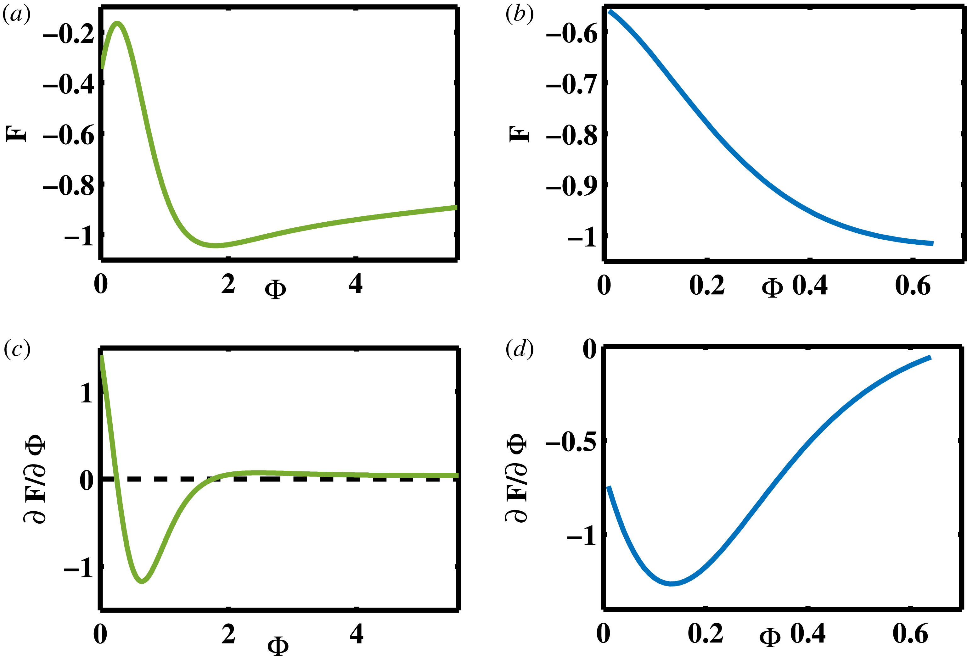
(a,b) and its first order derivatives (c,d); (a,c) for SSW; (b,d) for RSW.

The importance of the
 $F$
-analysis becomes imminent as we have found that the Sagdeev pseudopotential profile for a SSW in a magnetized plasma seems to appear in the vicinity of the singularity (§ 3.1). Figures 6(a) and 6(b) show the
 $F$
-variation for the SSW (curve (3), figure 1) and RSW (figure 3
b) respectively. The latter shows a monotonic variation (RSW) while for a SSW it distinctly fluctuates, showing a maximum and a minimum. In figures 6(c) and 6(d) we have further plotted the corresponding slopes (viz.,
 $\unicode[STIX]{x2202}F/\unicode[STIX]{x2202}\unicode[STIX]{x1D6F7}$
) for the SSW and RSW respectively. The latter (figure 6
d) shows a smooth but nonlinear variation profile where it initially decreases, and then, after attaining a minimum, increases once again. Throughout the variation, it remains always negative as expected from figure 6(b). The slope for SSW (figure 6
c), on the other hand, is non-monotonic and fluctuates between positive and negative values. The fluctuating
 $\unicode[STIX]{x2202}F/\unicode[STIX]{x2202}\unicode[STIX]{x1D6F7}$
may well be considered as another valid description of a SSW in the presence of the magnetic field.
According to the above analysis, as the slope of
 $F$
fluctuates from positive to negative, it ensures a SSW solution provided
 $F\neq 0$
throughout the range of
 $\unicode[STIX]{x1D6F7}$
i.e.
 $(0\leqslant \unicode[STIX]{x1D6F7}\leqslant \unicode[STIX]{x1D6F7}_{0})$
. The point of fluctuation for
 $F$
, or, alternatively, the first root of
 $\unicode[STIX]{x2202}F/\unicode[STIX]{x2202}\unicode[STIX]{x1D6F7}$
in figure 6(c), further determines the position of the auxiliary subwell, and hence the type of the transition which is Type IIA for the present case. Equation (A 6) shows that the variation of
 $F$
depends implicitly on both the bulk electron concentration (
 $N_{es}$
) and its rate of change (
 $\text{d}N_{es}/\text{d}\unicode[STIX]{x1D6F7}$
). Although the physical implication of
 $F$
is not quite clear yet, we may well conjecture that the variations of
 $F$
and
 $\unicode[STIX]{x2202}F/\unicode[STIX]{x2202}\unicode[STIX]{x1D6F7}$
, together, form a proxy of the derivative analysis for a magnetized plasma. Not only does this ensure the feasibility of the solution by ruling out pseudopotentials with singularities, but also the fluctuating nature of the SSW and other extra-nonlinear solutions appear to be imprinted in the variation of these two quantities. We thus propose the following two conditions to ensure a SSW solution in a magnetized plasma
 $$\begin{eqnarray}\displaystyle & \displaystyle F\neq 0\quad \text{for }0\leqslant \unicode[STIX]{x1D6F7}\leqslant \unicode[STIX]{x1D6F7}_{0}, & \displaystyle\end{eqnarray}$$
 $$\begin{eqnarray}\displaystyle & \displaystyle \frac{\unicode[STIX]{x2202}F}{\unicode[STIX]{x2202}\unicode[STIX]{x1D6F7}}\bigg|_{\unicode[STIX]{x1D6F7}=\unicode[STIX]{x1D6F7}_{a}}\geqslant 0\quad \text{for }0<\unicode[STIX]{x1D6F7}_{a}<\unicode[STIX]{x1D6F7}_{0}. & \displaystyle\end{eqnarray}$$
If the second condition is satisfied for any
 $\unicode[STIX]{x1D6F7}=\unicode[STIX]{x1D6F7}_{a}$
within the range then it ensures that there is an auxiliary subwell at
 $\unicode[STIX]{x1D6F7}=\unicode[STIX]{x1D6F7}_{a}$
which in turn confirms the presence, or the onset of, the SSW.
Varghese & Ghosh (Reference Varghese and Ghosh2016) have quantified the SSW by assigning 4 roots to the first derivative of Sagdeev pseudopotential. Our solution satisfies their condition which further validates our claim of the magnetized electron acoustic SSW associated with curve (3) (figure 1). However the conditions for any higher order derivatives and their morphology differ for the magnetized plasma. Hence we propose the
 $F$
analysis as a better candidate to examine the SSW in the case of a magnetized plasma. We also propose the
 $F$
-analysis to be a routine tool to identify all the extra-nonlinear structures for a magnetized plasma which will complement the derivative analysis proposed by Varghese & Ghosh (Reference Varghese and Ghosh2016).
3.3.2 Phase portrait
Phase portraits were another criterion which have been routinely studied by Dubinov et al. (Reference Dubinov, Kolotkov and Sazonkin2012) (Dubinov & Kolotkov Reference Dubinov and Kolotkov2012a
,Reference Dubinov and Kolotkov
b
,Reference Dubinov and Kolotkov
c
), and many others (Verheest et al.
Reference Verheest, Hellberg and Kourakis2013a
,Reference Verheest, Hellberg and Kourakis
b
,Reference Verheest, Hellberg and Kourakis
c
; Verheest & Hellberg Reference Verheest and Hellberg2015) to identify the SSW solution. We recall that (2.18) is considered as an analogy of a particle in a potential well, while
 $\unicode[STIX]{x1D6F9}$
is the pseudopotential, and
 $\unicode[STIX]{x1D6F7}$
and
 $\unicode[STIX]{x1D702}$
are analogous to the pseudo position and pseudo time respectively. Following that analogy, we have delineated the phase portrait of the ‘pseudoparticle’ where
 $\text{d}\unicode[STIX]{x1D6F7}/\text{d}\unicode[STIX]{x1D702}$
has been assumed to be analogous to the velocity of a real particle within a potential well. The closed trajectory ensures an oscillating or periodic solution while the saddle point confirms a solitary structure for the wave.
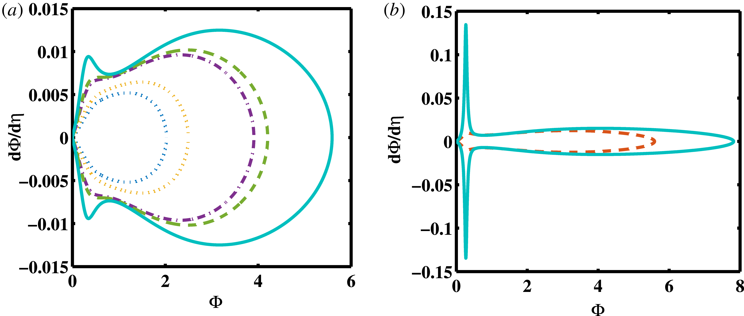
Phase portrait for the chosen parametric regime; (a) for
 $0.7\leqslant M_{\text{eff}}\leqslant 0.81$
, and (b) for
 $M_{\text{eff}}=0.81$
and
 $0.84$
.

Figure 7(a,b) represents the phase portraits for the chosen parametric regime. For the sake of clarity, the more ‘regular’, or less spiky, solutions have been shown in figure 7(a) while the solutions with deep and spiky auxiliary subwells have been presented separately in figure 7(b). The respective effective Mach numbers for figure 7(a) comprise
 $0.7\leqslant M_{\text{eff}}\leqslant 0.81$
while those in figure 7(b) are
 $M_{\text{eff}}=0.81$
and
 $0.84$
respectively. Beyond
 $M_{\text{eff}}=0.84$
the solution ceases to exist due to the singularity. The dash-dotted curve in figure 7(a) corresponds to one of the prominent gVSW (curve (1) in figure 1) and the dashed curve corresponds to the CoI, both presenting deformations in the otherwise smooth curves of the phase portrait. The bump appears to be more prominent from
 $M_{\text{eff}}=0.77$
onwards. In figure 7(b), the solid curve corresponds to the effective Mach number
 $M_{\text{eff}}=0.84$
which lies sufficiently close to the singularity and the dashed curve corresponds to
 $M_{\text{eff}}=0.81$
which represents the SSW. For a SSW solution and beyond, the depth of its wiggle increases rapidly with the increasing
 $M_{\text{eff}}$
, which supersedes their extent along
 $\unicode[STIX]{x1D6F7}$
in their phase portraits, turning it a highly elongated, spindle shaped profile. Especially the outermost phase portrait in figure 7(b) is worth noting. As per our previous analyses in § 3.1, the solution remains finite and physical, yet it is exceptionally spiky, with an almost horn-like subwell. This arises due to a very small, yet finite, value of
 $|F_{\text{max}}|$
which gives a clear signature of the approaching singularity. The feature is unique for the magnetized plasma and has no counterpart so far for a parallel propagation of the wave.
Dubinov et al. (Reference Dubinov, Kolotkov and Sazonkin2012) have previously argued that a SSW necessarily appears beyond the separatrix. In the present case, there is no such separatrix. This is to note that the previously reported separatrix was associated with the DL solution. In other words, only for a Type I transition the associated phase portrait will have any separatrix. Since no intermediate DL solution is involved in a Type II transition, there will be no separatrix either and the phase portrait will simply have closed phase trajectories. A phase portrait presented by Verheest et al. (Reference Verheest, Hellberg and Kourakis2013a ) also indicated a similar trend. This means that the appearance or the absence of a separatrix will readily confirm the type of the transition, viz., Type I or Type II respectively, but its presence does not imply a necessary condition for the existence of the aforementioned extra-nonlinear structures, including the SSWs, and cannot be considered as a generic condition for their existence.
Figure 7(a,b) further confirms that the present transition process does not belong to Type I but resembles Type II. The uniqueness of the extra-nonlinear solutions lie in their deformity of the phase portraits rather than the separatrix. A comparison with previously reported phase portraits for SSWs ensures the expected lateral inversion of the wiggles to the lower potential for the present case. This trend may well be attributed to the effect of the magnetic field on the SSW.
4 Discussion and conclusions
An electron acoustic SSW solution has been identified for a four component magnetized plasma where the ions are following Boltzmann distributions and the plasma is traversed by a warm beam of electrons. This is the first result of the SSW in a magnetized plasma where the solution is free from any ambiguity arising due to the singularity. This is also the first report of an electron acoustic SSW confirming extra-nonlinear structures for a higher frequency mode as well. We have developed an analytical formalism to identify a SSW in a magnetized plasma on the basis of the variation of
 $F$
and its derivative with
 $\unicode[STIX]{x1D6F7}$
. It reveals that, for a SSW, its derivative fluctuates between a positive and negative values while for a RSW it always remains negative. A comparison with the previously proposed derivative analysis (Varghese & Ghosh Reference Varghese and Ghosh2016) indicates that the fluctuating
 $\unicode[STIX]{x2202}F/\unicode[STIX]{x2202}\unicode[STIX]{x1D6F7}$
plays a role which is implicitly analogous to that of the charge separation for an unmagnetized plasma. It is found that the derivative analysis itself deviates for its higher orders in the presence of the magnetic field. To address this lacuna and to complement the previous formalism, we propose the
 $F$
-analysis as a routine tool to characterize SSWs in a magnetized plasma.
The one major influence of the presence of the magnetic field is the change in the relative position of the auxiliary subwell. We have defined the extra subwell as auxiliary vis-á-vis the main one where the former causes the wiggle of the otherwise bipolar electric field. Apart from the
 $F$
-analysis, the low potential auxiliary subwell further manifests itself in its potential and electric field profiles as well as the phase portrait of the pseudoparticle. The said ‘lateral inversion’ in the position of the auxiliary subwell causes the wiggle to appear at the base of the potential profile instead at the higher potential. Whether such lateral inversion is generic for any magnetized plasma is an open question at present and may be addressed later in the due course.
The major two characteristics of the magnetized plasma, a low potential auxiliary subwell and a fluctuating
 $F$
, are found to be correlated and they together carry the information of the imminent singularity of the pseudopotential. This also get manifested in the phase portrait which is devoid of any separatrix but shows a continuous deformation near the saddle point. As the amplitude increases, instead of the ‘smoothening of the wiggle’ (Verheest et al.
Reference Verheest, Hellberg and Kourakis2013a
; Steffy & Ghosh Reference Steffy and Ghosh2017), it shoots up to a spiky ‘horn’-like structure leading to the singularity and the termination of the physical solution. That manifests itself in the highly elongated phase portraits near the termination. The particular type of transition to SSW is called Type IIA where II assures the absence of an intermediate DL solution while A denotes the position of the auxiliary subwell which is near to the lower potential.
Theoretically, a SSW in a magnetized plasma can be an excellent probe for the imminent singularity of the system. It also looks like the presence of the magnetic field broadens the feasibility of finding an SSW solution with a flexible parametric regime. The range of the solution further increased due to the rarefaction of the oscillating species. Such conditions may be more viable to detect these structures in the laboratory or space plasmas. More specifically, magnetospheric boundary layers are known to be dotted with numerous ESWs and may be a hotbed of detecting such structures. The organized nonlinear structures are known to play a significant role in the transport and the trapping of the particles. A more generic theory of SSW vis-á-vis its mother structure, the solitary wave, would thus enhance its applicability to other physical systems and would also throw light in its internal nonlinear dynamics.
Acknowledgements
The authors acknowledge B. Buti (Buti Foundation) and F. Verheest (Sterrenkundig Observatorium, Universiteit Gent, Belgium) for their helpful discussions. One of the authors, T.K., thanks G. S. Lakhina, S. V. Singh and T. Sreeraj (Indian Institute of Geomagnetism) for their valuable suggestions. The authors would like to thank the Director of Indian Institute of Geomagnetism for providing all the necessary facilities for carrying out this work.
Appendix A
The numerator of (2.19) is given by
 $$\begin{eqnarray}\displaystyle L_{e}(\unicode[STIX]{x1D6F7}) & = & \displaystyle \left[-k_{y}^{2}\unicode[STIX]{x1D6F7}+\frac{1}{2}M_{\text{eff}}^{2}\left(\frac{S_{e}}{N_{es}}\right)^{2}+3h_{e}+w_{e}\right]\nonumber\\ \displaystyle & & \displaystyle +\,k_{z}^{2}\left[-h_{e}+\frac{1}{N_{es}}(\unicode[STIX]{x1D70E}_{es}S_{e}-S_{e}^{\prime })+\frac{1}{2}\left(\frac{w_{e}}{M_{\text{eff}}}\right)^{2}\right],\end{eqnarray}$$
where
 $$\begin{eqnarray}\left.\begin{array}{@{}c@{}}S_{e}=N_{es}-1,\quad S_{e}^{\prime }=\widetilde{N}_{es}-\unicode[STIX]{x1D6FF},\quad \unicode[STIX]{x1D6FF}=\widetilde{N}_{es}\big|_{\unicode[STIX]{x1D6F7}=0};\\ h_{e}={\displaystyle \frac{\unicode[STIX]{x1D70E}_{es}(N_{es}^{2}-1)}{2}},\quad t=\unicode[STIX]{x1D70E}_{es}(N_{es}^{3}-1),\quad \text{and}\quad w_{e}=S_{e}^{\prime }-t.\end{array}\right\}\end{eqnarray}$$
Also
 $$\begin{eqnarray}\displaystyle & \displaystyle N_{es}=\frac{1}{\unicode[STIX]{x1D70C}_{es}}[n_{i}-\unicode[STIX]{x1D70C}_{eb}N_{eb}], & \displaystyle\end{eqnarray}$$
 $$\begin{eqnarray}\displaystyle & \displaystyle N_{eb}=\frac{1}{2\sqrt{3\unicode[STIX]{x1D70E}_{eb}}}\left[(M_{b+}^{2}+2\unicode[STIX]{x1D6F7})^{1/2}-(M_{b-}^{2}+2\unicode[STIX]{x1D6F7})^{1/2}\right], & \displaystyle\end{eqnarray}$$
where
 $$\begin{eqnarray}M_{b\pm }=\left(\frac{M_{\text{eff}}-k_{z}U_{eb}}{k_{z}}\right)\pm \sqrt{3\unicode[STIX]{x1D70E}_{eb}}.\end{eqnarray}$$
The denominator of (2.19) is given by
 $$\begin{eqnarray}F=\frac{\text{d}f}{\text{d}\unicode[STIX]{x1D6F7}}=\left(3\unicode[STIX]{x1D70E}_{es}N_{es}-\frac{M_{\text{eff}}^{2}}{N_{es}^{3}}\right)\frac{\text{d}N_{es}}{\text{d}\unicode[STIX]{x1D6F7}}-1,\end{eqnarray}$$
where
 $$\begin{eqnarray}f=\frac{1}{2}\left(\frac{M_{\text{eff}}^{2}}{N_{es}^{2}}+3\unicode[STIX]{x1D70E}_{es}N_{es}^{2}\right)-\unicode[STIX]{x1D6F7}.\end{eqnarray}$$
The first derivative of
 $F$
in figure 6 is given by
 $$\begin{eqnarray}\frac{\unicode[STIX]{x2202}F}{\unicode[STIX]{x2202}\unicode[STIX]{x1D6F7}}=\left[3\unicode[STIX]{x1D70E}_{es}+\frac{3M_{\text{eff}}^{2}}{N_{es}^{4}}\right]\left(\frac{\text{d}N_{es}}{\text{d}\unicode[STIX]{x1D6F7}}\right)^{2}+\left[3\unicode[STIX]{x1D70E}_{es}N_{es}-\frac{M_{\text{eff}}^{2}}{N_{es}^{3}}\right]\left(\frac{\text{d}^{2}N_{es}}{\text{d}\unicode[STIX]{x1D6F7}^{2}}\right).\end{eqnarray}$$