1 Introduction
There is a wealth of literature describing the fluid dynamics induced by the motion of a flexible body through a fluid flow. In most studies the body motion is bending dominated, with a moderate bending modulus, but essentially inextensible (Taneda Reference Taneda1968; Kornecki, Dowell & O’Brien Reference Kornecki, Dowell and O’Brien1976; Zhang et al. Reference Zhang, Childress, Libchaber and Shelley2000; Watanabe et al. Reference Watanabe, Suzuki, Sugihara and Sueoka2002; Zhu & Peskin Reference Zhu and Peskin2002; Argentina & Mahadevan Reference Argentina and Mahadevan2005; Shelley, Vandenberghe & Zhang Reference Shelley, Vandenberghe and Zhang2005; Eloy, Souilliez & Schouveiler Reference Eloy, Souilliez and Schouveiler2007; Alben Reference Alben2008b; Alben & Shelley Reference Alben and Shelley2008; Eloy et al. Reference Eloy, Lagrange, Souilliez and Schouveiler2008; Michelin, Smith & Glover Reference Michelin, Smith and Glover2008; Shelley & Zhang Reference Shelley and Zhang2011). A smaller number of studies, including this one, consider softer materials – extensible membranes – that have a negligible bending modulus, and undergo significant stretching in a fluid flow (Newman & Paidoussis Reference Newman and Paidoussis1991; Lian & Shyy Reference Lian and Shyy2005; Sygulski Reference Sygulski2007; Song et al. Reference Song, Tian, Israeli, Galvao, Bishop, Swartz and Breuer2008; Tiomkin & Raveh Reference Tiomkin and Raveh2017; Tzezana & Breuer Reference Tzezana and Breuer2019). Examples are rubber, textile fabric or the skin of swimming and flying animals (Newman Reference Newman1987; Lian et al. Reference Lian, Shyy, Viieru and Zhang2003; Lauder et al. Reference Lauder, Madden, Mittal, Dong and Bozkurttas2006; Cheney et al. Reference Cheney, Konow, Bearnot and Swartz2015).
Here we extend our model of an inextensible bending body with a vortex sheet wake (Alben Reference Alben2008a, Reference Alben2009) to an extensible membrane. Our previous work investigated the nonlinear dynamics of a periodically pitching flexible body in a fluid stream (Alben Reference Alben2009) and the flapping-flag instability (Alben & Shelley Reference Alben and Shelley2008), among many other studies of this problem (Tang, Yamamoto & Dowell Reference Tang, Yamamoto and Dowell2003; Shelley et al. Reference Shelley, Vandenberghe and Zhang2005; Eloy et al. Reference Eloy, Souilliez and Schouveiler2007; Michelin et al. Reference Michelin, Smith and Glover2008; Huang & Sung Reference Huang and Sung2010; Chen et al. Reference Chen, Jia, Wu, Yin and Ma2014; Alben Reference Alben2015). As bending rigidity is decreased below the flutter threshold, the flag transitions from periodic to chaotic dynamics. Our model includes the separation of vortex sheets at sharp edges (Krasny Reference Krasny1991; Nitsche & Krasny Reference Nitsche and Krasny1994; Jones Reference Jones2003; Jones & Shelley Reference Jones and Shelley2005), and regularizes free vortex sheets to avoid singularities (Chorin & Bernard Reference Chorin and Bernard1973; Krasny Reference Krasny1986; Brady, Leonard & Pullin Reference Brady, Leonard and Pullin1998; Nitsche, Taylor & Krasny Reference Nitsche, Taylor and Krasny2003; Alben Reference Alben2010).
In this model, vortex sheets approximate the thin viscous boundary layers along the body, which are advected from its trailing edge into the flow downstream. This can be regarded as the inviscid limit of the viscous flow, and gives a good representation of the large-scale features of the flow and the vortex wake dynamics at Reynolds numbers of  $O$(
 $10^{2}$–
 $10^{5}$) (Nitsche & Krasny Reference Nitsche and Krasny1994; Shukla & Eldredge Reference Shukla and Eldredge2007; Sheng et al. Reference Sheng, Ysasi, Kolomenskiy, Kanso, Nitsche and Schneider2012; Xu, Nitsche & Krasny Reference Xu, Nitsche and Krasny2017). These flows are challenging to simulate directly due to the need to resolve sharp layers of vorticity in the vicinity of an unsteady, possibly deforming solid boundary. The immersed boundary method (Peskin Reference Peskin2002; Zhu & Peskin Reference Zhu and Peskin2002; Griffith & Peskin Reference Griffith and Peskin2005; Taira & Colonius Reference Taira and Colonius2007; Ghias, Mittal & Dong Reference Ghias, Mittal and Dong2007; Tytell et al. Reference Tytell, Hsu, Williams, Cohen and Fauci2010; Hamlet, Santhanakrishnan & Miller Reference Hamlet, Santhanakrishnan and Miller2011; Tian et al. Reference Tian, Luo, Zhu, Liao and Lu2011) can successfully simulate this class of problems. Very fine grids are needed to resolve the vorticity, and these are refined adaptively for efficiency (Roma, Peskin & Berger Reference Roma, Peskin and Berger1999; Griffith et al. Reference Griffith, Hornung, McQueen and Peskin2007). However, by only computing flow quantities on one-dimensional contours (the body and the vortex sheet wake), the vortex sheet model is typically much less expensive to compute when the far-field wake is approximated, as described in appendix B.
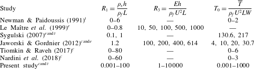
The focus of the present study is extensible membrane flutter: how a membrane initially aligned with a fluid flow becomes unstable to transverse deflections and eventually reaches steady-state large-amplitude dynamics. Large-amplitude membrane flutter can affect the performance of membrane aircraft (Lian & Shyy Reference Lian and Shyy2005; Hu, Tamai & Murphy Reference Hu, Tamai and Murphy2008; Stanford et al. Reference Stanford, Ifju, Albertani and Shyy2008; Jaworski & Gordnier Reference Jaworski and Gordnier2012; Piquee et al. Reference Piquee, López, Breitsamter, Wüchner and Bletzinger2018; Schomberg et al. Reference Schomberg, Gerland, Liese, Wünsch and Ruetten2018; Tzezana & Breuer Reference Tzezana and Breuer2019), sails (Colgate Reference Colgate1996; Kimball Reference Kimball2009), pneumatic membrane structures such as hanging roofs (Haruo Reference Haruo1975; Knudson Reference Knudson1991; Sygulski Reference Sygulski1996, Reference Sygulski1997, Reference Sygulski2007), and can occur in the human palate, resulting in snoring (Ellis, Williams & Shneerson Reference Ellis, Williams and Shneerson1993; Huang Reference Huang1995a,Reference Huangb; Wang, Rebeiz & Shapshay Reference Wang, Rebeiz and Shapshay2002; Howell et al. Reference Howell, Lucey, Carpenter and Pitman2009). The initial small-amplitude stage of the flutter instability has been the focus of several experimental, theoretical and numerical studies, summarized in table 1. We classify these and the present study in terms of three dimensionless parameters: membrane mass density, stretching modulus and pretension. The present simulations allow us to consider wide ranges of the parameters including those of the previous studies. Newman & Paidoussis (Reference Newman and Paidoussis1991) used an infinite periodic membrane model with a low-mode approximation and found that stability is lost through divergence. Le Maître, Huberson & De Cursi (Reference Le Maître, Huberson and De Cursi1999) used a vortex sheet model to study a more complex situation – the motions of a sail membrane under harmonic perturbations of the trailing edge and with randomly perturbed inflow velocities. Sygulski (Reference Sygulski2007) studied the membrane flutter threshold and divergence modes theoretically, with some experimental validation. Tiomkin & Raveh (Reference Tiomkin and Raveh2017) presented a more detailed flutter threshold calculation using an inviscid, small amplitude vortex sheet model. Nardini, Illingworth & Sandberg (Reference Nardini, Illingworth and Sandberg2018) compared a reduced-order model with direct numerical simulations to study the effect of Reynolds number on the flutter stability threshold and small-amplitude membrane deflection modes. So far there has been relatively little work on the large-amplitude dynamics following the initial flutter instability, and this is the focus of the present work.
Summary of parameter ranges used in previous and current membrane studies. Computational ( $^{c}$), experimental (
 $^{e}$) or theoretical (
 $^{t}$) ranges of the dimensionless body mass density
 $R_{1}$, stretching modulus
 $R_{3}$ and pretension
 $T_{0}$, defined in § 2.1.

Another main topic of fluid-membrane interaction studies is bio-inspired propulsion. Piquee et al. (Reference Piquee, López, Breitsamter, Wüchner and Bletzinger2018) studied how a membrane wing adjusts its shape to fluid pressure loading at various angles of attack. Tzezana & Breuer (Reference Tzezana and Breuer2019) coupled thin airfoil theory with a membrane equation to study the effects of wing compliance, inertia and flapping kinematics on aerodynamic performance. Jaworski & Gordnier (Reference Jaworski and Gordnier2012) studied a heaving and pitching membrane airfoil in a fluid stream numerically at Reynolds number 2500, and found elastic modulus and prestress parameters that led to enhanced thrust and propulsive efficiency. The passive adaptivity of a membrane wing has the potential to increase lift forces and delay the occurrence of stall to higher angles of attack for micro-air vehicles (MAVs) (Lian & Shyy Reference Lian and Shyy2005; Hu et al. Reference Hu, Tamai and Murphy2008; Stanford et al. Reference Stanford, Ifju, Albertani and Shyy2008). Schomberg et al. (Reference Schomberg, Gerland, Liese, Wünsch and Ruetten2018) used electrostatic forces to control a membrane shape and delay the transition from a laminar boundary layer, reducing viscous drag. Here, however, we focus solely on the flutter problem and defer propulsion-related dynamics to future work.
2 Membrane-vortex-sheet model
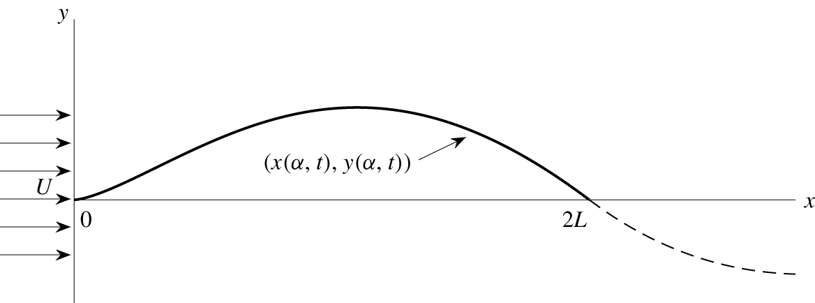
We first consider the motion of an extensible membrane that is fixed at two endpoints and held in a two-dimensional fluid flow, like much of the previous work. A uniform background flow is prescribed with velocity  $U$, directed parallel to the chord connecting the endpoints (see figure 1). The instantaneous position of the membrane is given by
 $\boldsymbol{X}(\unicode[STIX]{x1D6FC},t)=(x(\unicode[STIX]{x1D6FC},t),y(\unicode[STIX]{x1D6FC},t))$, parameterized by the material coordinate
 $\unicode[STIX]{x1D6FC},-L\leqslant \unicode[STIX]{x1D6FC}\leqslant L$ (
 $L$ is half the chord length) and time
 $t$. It is convenient to also describe the membrane position in complex notation,
 $\unicode[STIX]{x1D701}(\unicode[STIX]{x1D6FC},t)=x(\unicode[STIX]{x1D6FC},t)+\text{i}y(\unicode[STIX]{x1D6FC},t)$. The inviscid flow can be represented by a vortex sheet – a curve across which the tangential velocity component is discontinuous (Saffman Reference Saffman1992) – and whose position and strength evolve in time. The vortex sheet consists of two parts. One is ‘bound’ (it coincides with the membrane, for
 $-L\leqslant \unicode[STIX]{x1D6FC}\leqslant L$), and the other is ‘free,’ emanating from the trailing edge of the membrane at
 $\unicode[STIX]{x1D6FC}=L$. The bound and free vortex sheets have strength densities denoted by
 $\unicode[STIX]{x1D6FE}$ and positions denoted by
 $\unicode[STIX]{x1D701}$.
Schematic diagram of a flexible membrane (solid curved line) at an instant in time. Here  $2L$ is the chord length (the distance between the endpoints),
 $U$ is the oncoming flow velocity,
 $(x(\unicode[STIX]{x1D6FC},t),y(\unicode[STIX]{x1D6FC},t))$ is the membrane position and the dashed line is the free vortex sheet wake.

The membrane dynamics are described by the unsteady extensible elastica equation with body inertia, stretching resistance and fluid pressure loading (Tadjbakhsh Reference Tadjbakhsh1966), obtained by writing a force balance equation for a small section of membrane lying between  $\unicode[STIX]{x1D6FC}$ and
 $\unicode[STIX]{x1D6FC}+\unicode[STIX]{x0394}\unicode[STIX]{x1D6FC}$:
 $$\begin{eqnarray}\unicode[STIX]{x1D70C}_{s}hW\unicode[STIX]{x2202}_{tt}\unicode[STIX]{x1D701}(\unicode[STIX]{x1D6FC},t)\unicode[STIX]{x0394}\unicode[STIX]{x1D6FC}=T(\unicode[STIX]{x1D6FC}+\unicode[STIX]{x0394}\unicode[STIX]{x1D6FC},t)\hat{\boldsymbol{s}}-T(\unicode[STIX]{x1D6FC},t)\hat{\boldsymbol{s}}-[p](\unicode[STIX]{x1D6FC},t)\hat{\boldsymbol{n}}W(s(\unicode[STIX]{x1D6FC}+\unicode[STIX]{x0394}\unicode[STIX]{x1D6FC},t)-s(\unicode[STIX]{x1D6FC},t)).\end{eqnarray}$$
Dividing by  $\unicode[STIX]{x0394}\unicode[STIX]{x1D6FC}$ and taking the limit
 $\unicode[STIX]{x0394}\unicode[STIX]{x1D6FC}\rightarrow 0$, we obtain
 $$\begin{eqnarray}\unicode[STIX]{x1D70C}_{s}hW\unicode[STIX]{x2202}_{tt}\unicode[STIX]{x1D701}(\unicode[STIX]{x1D6FC},t)=\unicode[STIX]{x2202}_{\unicode[STIX]{x1D6FC}}(T(\unicode[STIX]{x1D6FC},t)\hat{\boldsymbol{s}})-[p](\unicode[STIX]{x1D6FC},t)W\unicode[STIX]{x2202}_{\unicode[STIX]{x1D6FC}}s\hat{\boldsymbol{n}},\end{eqnarray}$$
where  $\unicode[STIX]{x1D70C}_{s}$ is the mass per unit volume of the undeflected membrane,
 $h$ is its thickness and
 $W$ is its out-of-plane width, all uniform along the length. The material coordinate
 $\unicode[STIX]{x1D6FC}\in [-L,L]$ is the
 $x$-coordinate of the membrane in the initial flat, uniformly prestretched state. Other quantities that appear in (2.2) are
 $\hat{\boldsymbol{s}},\hat{\boldsymbol{n}}\in \mathbb{C}$, which represent the unit vectors tangent and normal to the membrane, respectively,
 $$\begin{eqnarray}\hat{\boldsymbol{s}}=\unicode[STIX]{x2202}_{\unicode[STIX]{x1D6FC}}\unicode[STIX]{x1D701}(\unicode[STIX]{x1D6FC},t)/\unicode[STIX]{x2202}_{\unicode[STIX]{x1D6FC}}s(\unicode[STIX]{x1D6FC},t)=\text{e}^{\text{i}\unicode[STIX]{x1D703}(\unicode[STIX]{x1D6FC},t)}\quad \text{and}\quad \hat{\boldsymbol{n}}=\text{i}\hat{\boldsymbol{s}}=\text{i}\text{e}^{\text{i}\unicode[STIX]{x1D703}(\unicode[STIX]{x1D6FC},t)},\end{eqnarray}$$
with  $\unicode[STIX]{x1D703}(\unicode[STIX]{x1D6FC},t)$ the local tangent angle,
 $s(\unicode[STIX]{x1D6FC},t)$ the local arc length coordinate and
 $\unicode[STIX]{x1D705}(\unicode[STIX]{x1D6FC},t)=\unicode[STIX]{x2202}_{\unicode[STIX]{x1D6FC}}\unicode[STIX]{x1D703}/\unicode[STIX]{x2202}_{\unicode[STIX]{x1D6FC}}s$ the membrane’s curvature. Here
 $[p](\unicode[STIX]{x1D6FC},t)$ is the local pressure difference across the membrane, from the side toward which
 $\hat{\boldsymbol{n}}$ points to the other side.
The membrane tension  $T(\unicode[STIX]{x1D6FC},t)$ is given by linear elasticity (Carrier Reference Carrier1945, Reference Carrier1949; Narasimha Reference Narasimha1968; Nayfeh & Pai Reference Nayfeh and Pai2008), i.e.
 $$\begin{eqnarray}T(\unicode[STIX]{x1D6FC},t)=\overline{T}+EhW(\unicode[STIX]{x2202}_{\unicode[STIX]{x1D6FC}}s(\unicode[STIX]{x1D6FC},t)-1),\end{eqnarray}$$
where  $E$ is the Young’s modulus. Thus, the tension is a constant
 $\overline{T}$, the ‘pretension,’ in the (initial) undeflected equilibrium state
 $\unicode[STIX]{x1D701}(\unicode[STIX]{x1D6FC},0)=\unicode[STIX]{x1D6FC}$.
2.1 Non-dimensionalization
We non-dimensionalize the governing equations by the density of the fluid  $\unicode[STIX]{x1D70C}_{f}$, the half-chord
 $L$ and the imposed fluid flow velocity
 $U$. In particular, we use
 $$\begin{eqnarray}\tilde{t}=\frac{t}{L/U},\quad (\tilde{\unicode[STIX]{x1D701}},\tilde{\unicode[STIX]{x1D6FC}},\tilde{s})=\frac{(\unicode[STIX]{x1D701},\unicode[STIX]{x1D6FC},s)}{L},\quad \widetilde{[p]}=\frac{[p]}{\unicode[STIX]{x1D70C}_{f}U^{2}}.\end{eqnarray}$$
The membrane equation (2.2) becomes
 $$\begin{eqnarray}\frac{\unicode[STIX]{x1D70C}_{s}hU^{2}W}{L}\widetilde{\unicode[STIX]{x2202}_{tt}\unicode[STIX]{x1D701}}=\frac{1}{L}\widetilde{\unicode[STIX]{x2202}_{\unicode[STIX]{x1D6FC}}}[(\overline{T}+EhW(\widetilde{\unicode[STIX]{x2202}_{\unicode[STIX]{x1D6FC}}s}-1))\hat{\boldsymbol{s}}]-\unicode[STIX]{x1D70C}_{f}U^{2}W\widetilde{[p]}\widetilde{\unicode[STIX]{x2202}_{\unicode[STIX]{x1D6FC}}s}\hat{\boldsymbol{n}},\end{eqnarray}$$
with dimensionless quantities (and their dimensionless derivatives) denoted by tildes. Dividing (2.6) by  $\unicode[STIX]{x1D70C}_{f}U^{2}W$ throughout yields
 $$\begin{eqnarray}\frac{\unicode[STIX]{x1D70C}_{s}h}{\unicode[STIX]{x1D70C}_{f}L}\widetilde{\unicode[STIX]{x2202}_{tt}\unicode[STIX]{x1D701}}=\frac{1}{\unicode[STIX]{x1D70C}_{f}U^{2}LW}\widetilde{\unicode[STIX]{x2202}_{\unicode[STIX]{x1D6FC}}}[(\overline{T}+EhW(\widetilde{\unicode[STIX]{x2202}_{\unicode[STIX]{x1D6FC}}s}-1))\hat{\boldsymbol{s}}]-\widetilde{[p]}\widetilde{\unicode[STIX]{x2202}_{\unicode[STIX]{x1D6FC}}s}\hat{\boldsymbol{n}}.\end{eqnarray}$$
Thus, the dimensionless membrane equation (dropping tildes) is
 $$\begin{eqnarray}R_{1}\unicode[STIX]{x2202}_{tt}\unicode[STIX]{x1D701}-\unicode[STIX]{x2202}_{\unicode[STIX]{x1D6FC}}((T_{0}+R_{3}(\unicode[STIX]{x2202}_{\unicode[STIX]{x1D6FC}}s-1))\hat{\boldsymbol{s}})=-[p]\unicode[STIX]{x2202}_{\unicode[STIX]{x1D6FC}}s\hat{\boldsymbol{n}}.\end{eqnarray}$$
The dimensionless parameters of the membrane are
 $$\begin{eqnarray}R_{1}=\frac{\unicode[STIX]{x1D70C}_{s}h}{\unicode[STIX]{x1D70C}_{f}L},\quad T_{0}=\frac{\overline{T}}{\unicode[STIX]{x1D70C}_{f}U^{2}LW}\quad \text{and}\quad R_{3}=\frac{Eh}{\unicode[STIX]{x1D70C}_{f}U^{2}L},\end{eqnarray}$$
where  $R_{1}$,
 $T_{0}$ and
 $R_{3}$ are the dimensionless membrane mass density, pretension and stretching modulus, respectively. We assume that the thickness ratio
 $h/L$ is small, but
 $\unicode[STIX]{x1D70C}_{s}/\unicode[STIX]{x1D70C}_{f}$ may be large, so
 $R_{1}$ may assume any non-negative value. We have neglected bending rigidity, denoted
 $R_{2}$ in Alben & Shelley (Reference Alben and Shelley2008). In the extensible membrane regime studied here,
 $R_{3}$ is finite, so
 $R_{2}=R_{3}h^{2}/12L^{2}\rightarrow 0$ in the limit
 $h/L\rightarrow 0$. By contrast, the inextensible beam or plate regime studied previously (Tang et al. Reference Tang, Yamamoto and Dowell2003; Shelley et al. Reference Shelley, Vandenberghe and Zhang2005; Eloy et al. Reference Eloy, Souilliez and Schouveiler2007; Michelin et al. Reference Michelin, Smith and Glover2008; Huang & Sung Reference Huang and Sung2010; Chen et al. Reference Chen, Jia, Wu, Yin and Ma2014; Alben Reference Alben2015) has
 $R_{2}$ finite and
 $R_{3}\rightarrow +\infty$ as
 $(h/L)^{-2}$ in the limit
 $h/L\rightarrow 0$, resulting in inextensibility. We have also neglected the effects of rotary inertia and the Poisson ratio (the transverse contraction due to axial stretching), which have usually been neglected at leading order in nonlinear membrane models (Nayfeh & Pai Reference Nayfeh and Pai2008) and the aforementioned membrane studies. The rotary inertia and bending rigidity terms are given in Tadjbakhsh (Reference Tadjbakhsh1966), and those involving the Poisson ratio are given in Nayfeh & Pai (Reference Nayfeh and Pai2008).
For large-Reynolds-number flows, there are thin viscous boundary layers along the sides of the membrane. Across these boundary layers, the component of fluid velocity that is tangent to the membrane is brought to zero on the membrane (Batchelor Reference Batchelor1967). When the fluid in the boundary layer is advected off of the membrane’s trailing edge, a free shear layer forms (Saffman Reference Saffman1992; Alben Reference Alben2010). In the limit of large Reynolds number, the two boundary layers tend to vortex sheets which coincide as a single bound vortex sheet (approximating the body thickness as zero for the fluid computation). The free shear layer tends to a free vortex sheet (Saffman Reference Saffman1992). The free sheet circulation is defined as an integral of the vortex sheet strength  $\unicode[STIX]{x1D6FE}$ (the jump in the tangential component of the fluid velocity) over the free vortex sheet
 $$\begin{eqnarray}\unicode[STIX]{x1D6E4}(s,t)=-\int _{s}^{s_{max}}\unicode[STIX]{x1D6FE}(s^{\prime },t)\,\text{d}s^{\prime },\quad 0<s<s_{max},\end{eqnarray}$$
where  $s$ is the arc length along the free sheet, starting from 0 where the free sheet meets the membrane’s trailing edge and ending at
 $s_{max}$ at the free sheet’s far end. Following Jones (Reference Jones2003) and Alben (Reference Alben2009), we define the (negative of the) total circulation in the free sheet as
 $$\begin{eqnarray}\unicode[STIX]{x1D6E4}_{+}(t)=\unicode[STIX]{x1D6E4}(0,t)=-\int _{0}^{s_{max}}\unicode[STIX]{x1D6FE}(s,t)\,\text{d}s.\end{eqnarray}$$
The complex conjugate of the flow velocity  $\boldsymbol{u}=(u_{x},u_{y})$ at any point
 $z$ in the flow (not on the vortex sheets) can be calculated in terms of
 $\unicode[STIX]{x1D6FE}$ by integrating the vorticity in the bound and free vortex sheets against the Biot–Savart kernel (Saffman Reference Saffman1992), i.e.
 $$\begin{eqnarray}u_{x}(z)-\text{i}u_{y}(z)=1+\frac{1}{2\unicode[STIX]{x03C0}\text{i}}\int _{-1}^{1}\frac{\unicode[STIX]{x1D6FE}(\unicode[STIX]{x1D6FC},t)}{z-\unicode[STIX]{x1D701}(\unicode[STIX]{x1D6FC},t)}\unicode[STIX]{x2202}_{\unicode[STIX]{x1D6FC}}s(\unicode[STIX]{x1D6FC},t)\,\text{d}\unicode[STIX]{x1D6FC}+\frac{1}{2\unicode[STIX]{x03C0}\text{i}}\int _{0}^{s_{max}}\frac{\unicode[STIX]{x1D6FE}(s,t)}{z-\unicode[STIX]{x1D701}(s,t)}\,\text{d}s,\end{eqnarray}$$
with unity on the right-hand side representing the imposed background flow and the dimensionless material coordinate  $\unicode[STIX]{x1D6FC}$ ranging from
 $-1$ to 1 on the membrane. By Kelvin’s circulation theorem,
 $\unicode[STIX]{x1D6E4}$ is conserved at fixed material elements of the free vortex sheet. Thus, we reparameterize the free sheet position as
 $\unicode[STIX]{x1D701}(\unicode[STIX]{x1D6E4},t)$ and evolve the position at a fixed
 $\unicode[STIX]{x1D6E4}$ simply by following the local fluid velocity. This is done by taking the average of the limits of (2.12) as
 $z$ approaches
 $\unicode[STIX]{x1D701}(\unicode[STIX]{x1D6E4},t)$ from both sides (Saffman Reference Saffman1992):
 $$\begin{eqnarray}\frac{\unicode[STIX]{x2202}\overline{\unicode[STIX]{x1D701}}}{\unicode[STIX]{x2202}t}(\unicode[STIX]{x1D6E4},t)=1+\frac{1}{2\unicode[STIX]{x03C0}\text{i}}\int _{-1}^{1}\frac{\unicode[STIX]{x1D6FE}(\unicode[STIX]{x1D6FC},t)}{\unicode[STIX]{x1D701}(\unicode[STIX]{x1D6E4},t)-\unicode[STIX]{x1D701}(\unicode[STIX]{x1D6FC},t)}\unicode[STIX]{x2202}_{\unicode[STIX]{x1D6FC}}s(\unicode[STIX]{x1D6FC},t)\,\text{d}\unicode[STIX]{x1D6FC}-\frac{1}{2\unicode[STIX]{x03C0}\text{i}}\;\unicode[STIX]{x2A0D}-_{0}^{\unicode[STIX]{x1D6E4}_{+}(t)}\frac{\text{d}\unicode[STIX]{x1D6E4}^{\prime }}{\unicode[STIX]{x1D701}(\unicode[STIX]{x1D6E4},t)-\unicode[STIX]{x1D701}(\unicode[STIX]{x1D6E4}^{\prime },t)}.\end{eqnarray}$$
In (2.13),  $\unicode[STIX]{x2202}\overline{\unicode[STIX]{x1D701}}/\unicode[STIX]{x2202}t$ is the complex conjugate velocity at
 $\unicode[STIX]{x1D701}(\unicode[STIX]{x1D6E4},t)$, and the second integral is a Cauchy-principal-value integral. We have reparameterized the free sheet integral using
 $\unicode[STIX]{x1D6FE}\,\text{d}s=-\text{d}\unicode[STIX]{x1D6E4}$. This form of the integral appears in the Birkhoff–Rott equation for the evolution of a free vortex sheet (Saffman Reference Saffman1992; Jones Reference Jones2003; Pullin & Wang Reference Pullin and Wang2004; Jones & Shelley Reference Jones and Shelley2005). In this form
 $\text{d}\unicode[STIX]{x1D6E4}$ may have either sign.
We may solve for the bound vortex sheet strength  $\unicode[STIX]{x1D6FE}(\unicode[STIX]{x1D6FC},t)$ in terms of the membrane velocity by equating the components of the fluid and membrane velocities normal to the membrane (‘the kinematic condition’), which are found by taking the average of the limits of (2.13) as
 $z$ approaches the membrane from both sides:
 $$\begin{eqnarray}\displaystyle & & \displaystyle \mathit{Re}(\hat{\boldsymbol{n}}\unicode[STIX]{x2202}_{t}\overline{\unicode[STIX]{x1D701}}(\unicode[STIX]{x1D6FC},t))\nonumber\\ \displaystyle & & \displaystyle \quad =\mathit{Re}\left(\hat{\boldsymbol{n}}\left(1+\frac{1}{2\unicode[STIX]{x03C0}\text{i}}\;\unicode[STIX]{x2A0D}-_{-1}^{1}\frac{\unicode[STIX]{x1D6FE}(\unicode[STIX]{x1D6FC}^{\prime },t)\unicode[STIX]{x2202}_{\unicode[STIX]{x1D6FC}}s(\unicode[STIX]{x1D6FC}^{\prime },t)}{\unicode[STIX]{x1D701}(\unicode[STIX]{x1D6FC},t)-\unicode[STIX]{x1D701}(\unicode[STIX]{x1D6FC}^{\prime },t)}\,\text{d}\unicode[STIX]{x1D6FC}^{\prime }-\frac{1}{2\unicode[STIX]{x03C0}\text{i}}\int _{0}^{\unicode[STIX]{x1D6E4}_{+}(t)}\frac{\text{d}\unicode[STIX]{x1D6E4}^{\prime }}{\unicode[STIX]{x1D701}(\unicode[STIX]{x1D6FC},t)-\unicode[STIX]{x1D701}(\unicode[STIX]{x1D6E4}^{\prime },t)}\right)\right).\nonumber\\ \displaystyle & & \displaystyle\end{eqnarray}$$
When the left-hand side and the second integral on the right-hand side of (2.14) are known, the general solution  $\unicode[STIX]{x1D6FE}(\unicode[STIX]{x1D6FC},t)$ has inverse-square-root singularities at
 $\unicode[STIX]{x1D6FC}=\pm 1$. Therefore, we define
 $v(\unicode[STIX]{x1D6FC},t)$, the bounded part of
 $\unicode[STIX]{x1D6FE}(\unicode[STIX]{x1D6FC},t)$, by
 $$\begin{eqnarray}\unicode[STIX]{x1D6FE}(\unicode[STIX]{x1D6FC},t)=\frac{v(\unicode[STIX]{x1D6FC},t)}{\sqrt{1-\unicode[STIX]{x1D6FC}^{2}}}.\end{eqnarray}$$
An additional scalar constraint is required to uniquely specify the solution  $\unicode[STIX]{x1D6FE}$ (or
 $v$) to (2.14). It is the conservation of total circulation (Kelvin’s circulation theorem):
 $$\begin{eqnarray}\int _{-1}^{1}\unicode[STIX]{x1D6FE}\unicode[STIX]{x2202}_{\unicode[STIX]{x1D6FC}}s\,\text{d}\unicode[STIX]{x1D6FC}=\int _{-1}^{1}\frac{v(\unicode[STIX]{x1D6FC},t)}{\sqrt{1-\unicode[STIX]{x1D6FC}^{2}}}\unicode[STIX]{x2202}_{\unicode[STIX]{x1D6FC}}s\,\text{d}\unicode[STIX]{x1D6FC}=\unicode[STIX]{x1D6E4}_{+}(t).\end{eqnarray}$$
In (2.13) and (2.14) it is helpful to replace the free sheet integral with a regularized version to avoid singularities in the sheet curvature (Krasny Reference Krasny1986). The second integral in (2.13) becomes
 $$\begin{eqnarray}-\frac{1}{2\unicode[STIX]{x03C0}\text{i}}\;\unicode[STIX]{x2A0D}-_{0}^{\unicode[STIX]{x1D6E4}_{+}(t)}\frac{\overline{\unicode[STIX]{x1D701}(\unicode[STIX]{x1D6E4},t)-\unicode[STIX]{x1D701}(\unicode[STIX]{x1D6E4}^{\prime },t)}}{|\unicode[STIX]{x1D701}(\unicode[STIX]{x1D6E4},t)-\unicode[STIX]{x1D701}(\unicode[STIX]{x1D6E4}^{\prime },t)|^{2}+\unicode[STIX]{x1D6FF}(\unicode[STIX]{x1D6E4}^{\prime },t)^{2}}\,\text{d}\unicode[STIX]{x1D6E4}^{\prime },\end{eqnarray}$$
with a regularization parameter
 $$\begin{eqnarray}\unicode[STIX]{x1D6FF}(\unicode[STIX]{x1D6E4},t)=\unicode[STIX]{x1D6FF}_{0}(1-\text{e}^{-s(\unicode[STIX]{x1D6E4},t)^{2}/\unicode[STIX]{x1D700}^{2}}).\end{eqnarray}$$
The effect of  $\unicode[STIX]{x1D6FF}$ is to inhibit the growth of free sheet structures (e.g. inner turns of spirals) on scales smaller than
 $\unicode[STIX]{x1D6FF}$ while maintaining the shape and motion of the sheet on larger scales. Our choice of
 $\unicode[STIX]{x1D6FF}$ tends to 0 quadratically over a scale given by
 $\unicode[STIX]{x1D700}$ as the membrane trailing edge is approached, to decrease the effect of regularization on the flow near the trailing edge and the production of circulation (Alben Reference Alben2009, Reference Alben2010). Here we set
 $\unicode[STIX]{x1D700}$ to 0.4 and
 $\unicode[STIX]{x1D6FF}_{0}$ to 0.2, choices that make the effect of regularization on circulation production small without a significant increase in the total number of points needed to resolve the free sheet (Alben Reference Alben2010). The Kutta condition determines the rate of circulation production
 $\text{d}\unicode[STIX]{x1D6E4}_{+}(t)/\text{d}t$ by making the fluid velocity at the trailing edge finite. This means
 $\unicode[STIX]{x1D6FE}(1,t)$ must be finite, and, thus,
 $v(1,t)=0$ by (2.15).
The vortex sheet strength  $\unicode[STIX]{x1D6FE}(\unicode[STIX]{x1D6FC},t)$ is coupled to the pressure jump
 $[p](\unicode[STIX]{x1D6FC},t)$ across the membrane using a version of the unsteady Bernoulli equation written at a fixed material point on the membrane:
 $$\begin{eqnarray}\unicode[STIX]{x2202}_{\unicode[STIX]{x1D6FC}}s\unicode[STIX]{x2202}_{t}\unicode[STIX]{x1D6FE}+(\unicode[STIX]{x1D707}-\unicode[STIX]{x1D70F})\unicode[STIX]{x2202}_{\unicode[STIX]{x1D6FC}}\unicode[STIX]{x1D6FE}+\unicode[STIX]{x1D6FE}(\unicode[STIX]{x2202}_{\unicode[STIX]{x1D6FC}}\unicode[STIX]{x1D707}-\unicode[STIX]{x2202}_{\unicode[STIX]{x1D6FC}}s\unicode[STIX]{x1D708}\unicode[STIX]{x1D705})=\unicode[STIX]{x2202}_{\unicode[STIX]{x1D6FC}}[p].\end{eqnarray}$$
This equation is derived in appendix A, and generalizes the derivation in Alben (Reference Alben2012, appendix A) to the case of an extensible body.
In (2.19),  $\unicode[STIX]{x1D707}$ is the tangential component of the average flow velocity at the membrane,
 $$\begin{eqnarray}\unicode[STIX]{x1D707}(\unicode[STIX]{x1D6FC},t)=\mathit{Re}\left(\hat{\boldsymbol{s}}\left(1+\frac{1}{2\unicode[STIX]{x03C0}\text{i}}\;\unicode[STIX]{x2A0D}-_{-1}^{1}\frac{\unicode[STIX]{x1D6FE}(\unicode[STIX]{x1D6FC}^{\prime },t)\unicode[STIX]{x2202}_{\unicode[STIX]{x1D6FC}}s(\unicode[STIX]{x1D6FC}^{\prime },t)}{\unicode[STIX]{x1D701}(\unicode[STIX]{x1D6FC},t)-\unicode[STIX]{x1D701}(\unicode[STIX]{x1D6FC}^{\prime },t)}\,\text{d}\unicode[STIX]{x1D6FC}^{\prime }-\frac{1}{2\unicode[STIX]{x03C0}\text{i}}\int _{0}^{\unicode[STIX]{x1D6E4}_{+}(t)}\frac{\text{d}\unicode[STIX]{x1D6E4}^{\prime }}{\unicode[STIX]{x1D701}(\unicode[STIX]{x1D6FC},t)-\unicode[STIX]{x1D701}(\unicode[STIX]{x1D6E4}^{\prime },t)}\right)\right),\end{eqnarray}$$
and  $\unicode[STIX]{x1D70F}$ and
 $\unicode[STIX]{x1D708}$ are respectively the components of the membrane’s velocity tangent and normal to itself:
 $$\begin{eqnarray}\unicode[STIX]{x1D70F}(\unicode[STIX]{x1D6FC},t)=\mathit{Re}(\unicode[STIX]{x2202}_{t}\overline{\unicode[STIX]{x1D701}}(\unicode[STIX]{x1D6FC},t)\hat{\boldsymbol{s}});\quad \unicode[STIX]{x1D708}(\unicode[STIX]{x1D6FC},t)=\mathit{Re}(\unicode[STIX]{x2202}_{t}\overline{\unicode[STIX]{x1D701}}(\unicode[STIX]{x1D6FC},t)\hat{\boldsymbol{n}}).\end{eqnarray}$$
The pressure jump across the free sheet is zero, which yields
 $$\begin{eqnarray}[p]|_{\unicode[STIX]{x1D6FC}=1}=0,\end{eqnarray}$$
the boundary condition we use to integrate (2.19) and obtain  $[p](\unicode[STIX]{x1D6FC},t)$ on the membrane.
2.2 Boundary and initial conditions
We investigate three cases of boundary conditions at the two ends of the membrane, shown schematically in figure 2. In all three cases, the  $x$-coordinates of the ends are constant:
 $x(-1,t)=0$ and
 $x(1,t)=2$. In the first case, ‘fixed–fixed,’ the membrane is flat at
 $t=0$, and we set the deflection to zero at both ends of the membrane after a small initial perturbation. More precisely, we smoothly perturb
 $y$ at the leading edge slightly away from zero and relax it to zero exponentially in time, i.e.
 $$\begin{eqnarray}y(-1,t)=\unicode[STIX]{x1D70E}\left(\frac{t}{\unicode[STIX]{x1D702}}\right)^{3}\text{e}^{-(t/\unicode[STIX]{x1D702})^{3}},\end{eqnarray}$$
where  $\unicode[STIX]{x1D70E}$ is a constant chosen in the range
 $10^{-6}$–
 $10^{-3}$ (depending on whether small or large amplitude dynamics are studied) and
 $\unicode[STIX]{x1D702}=0.2$. We set the trailing edge deflection
 $y(1,t)$ to zero for all
 $t$. This is essentially the case considered by most previous studies of membrane flutter (Le Maître et al. Reference Le Maître, Huberson and De Cursi1999; Sygulski Reference Sygulski2007; Tiomkin & Raveh Reference Tiomkin and Raveh2017; Nardini et al. Reference Nardini, Illingworth and Sandberg2018), and here we find, surprisingly, that all physically reasonable deflected membrane states are steady (i.e. without oscillations). In the second case, ‘fixed–free,’ we again make the membrane flat initially and then set the leading edge position according to (2.23), but allow the trailing edge to deflect freely in the vertical direction. This is the classical free-end boundary condition for a membrane (Graff Reference Graff1975; Farlow Reference Farlow1993) and corresponds to the membrane end fixed to a massless ring that slides without friction along a vertical pole (see figure 2b). Without friction, the force from the pole on the ring at the membrane end is horizontal. The tension force from the membrane on the ring must also be horizontal, or else the ring would have an infinite vertical acceleration. Therefore,
 $\hat{\boldsymbol{s}}=\hat{\boldsymbol{e}}_{x}$ at the trailing edge or, equivalently,
 $\unicode[STIX]{x2202}_{\unicode[STIX]{x1D6FC}}y(1,t)=0$.
Schematic diagrams of the three sets of boundary conditions considered: fixed–fixed (a), fixed–free (b), and free–free (c).

Although well known in classical mechanics, free-end boundary conditions have not been studied much in membrane (as opposed to beam/plate) flutter problems. Tamai, Murphy & Hu (Reference Tamai, Murphy and Hu2008) studied membrane wings with partially free trailing edges and found that trailing edge fluttering may occur at relatively low angles of attack. Another recent experimental study found that membrane wing flutter can be enhanced by the vibrations of flexible leading and trailing edge supports (Arbós-Torrent, Ganapathisubramani & Palacios Reference Arbós-Torrent, Ganapathisubramani and Palacios2013). Partially free edges occur also in sails: the shape of a sail membrane can be controlled by altering the tension in cables running along its free edges (the ‘leech’ and ‘foot’) (Kimball Reference Kimball2009). Flutter can occur when the tension in these edges is sufficiently low (Colgate Reference Colgate1996). A related application is to energy harvesting by membranes mounted on tensegrity structures (networks of rigid rods and elastic fibres) and placed in fluid flows (Sunny, Sultan & Kapania Reference Sunny, Sultan and Kapania2014; Yang & Sultan Reference Yang and Sultan2016). In such cases the membrane ends have some degrees of freedom akin to the free-end boundary conditions defined above.
We will show that free ends allow for a wide range of unsteady membrane dynamics, unlike in the fixed–fixed case. Related work has studied the dynamics and flutter of membranes and cables under gravity with free ends (Triantafyllou & Howell Reference Triantafyllou and Howell1994; Manela & Weidenfeld Reference Manela and Weidenfeld2017). Here we neglect gravity to focus specifically on the basic flutter problem (Shelley & Zhang Reference Shelley and Zhang2011). Without gravity, some restriction on the motion of the free membrane ends is needed to avoid ill-posedness due to membrane compression (Triantafyllou & Howell Reference Triantafyllou and Howell1994). This is provided by the vertical poles in figure 2. Although this type of free-end boundary condition has mainly been studied theoretically, it has been realized experimentally by Kashy et al. (Reference Kashy, Johnson, McIntyre and Wolfe1997), with the membrane represented by an extensional spring that is tethered by steel wires to vertical supports.
In the third case, ‘free–free,’ both ends are free:  $\unicode[STIX]{x2202}_{\unicode[STIX]{x1D6FC}}y(-1,t)=\unicode[STIX]{x2202}_{\unicode[STIX]{x1D6FC}}y(1,t)=0$. Here the membrane is perturbed differently: it is initially set with a small non-zero slope,
 $$\begin{eqnarray}\unicode[STIX]{x1D701}(\unicode[STIX]{x1D6FC},0)=(\unicode[STIX]{x1D6FC}+1)(1+\text{i}\unicode[STIX]{x1D70E})\end{eqnarray}$$
for  $\unicode[STIX]{x1D70E}=10^{-3}$.
3 Numerical results and discussion
We now describe the range of dynamics of the extensible membrane with the three sets of boundary conditions. In each case, we first present the flutter stability region for the flat membrane in the  $R_{1}$–
 $T_{0}$ plane (it is independent of
 $R_{3}$ because it depends only on the small-deflection behavior). We then consider the large-amplitude dynamics using three main quantities to characterize them. One is the time-averaged deflection of the membrane,
 $$\begin{eqnarray}\langle y_{defl}\rangle \equiv \frac{1}{t_{2}}\int _{t_{1}}^{t_{1}+t_{2}}\left(\max _{-1\leqslant \unicode[STIX]{x1D6FC}\leqslant 1}y(\unicode[STIX]{x1D6FC},t)-\min _{-1\leqslant \unicode[STIX]{x1D6FC}\leqslant 1}y(\unicode[STIX]{x1D6FC},t)\right)\,\text{d}t,\end{eqnarray}$$
where  $t_{1}$ and
 $t_{2}$ are sufficiently large (typically 50–100) that
 $\langle y_{defl}\rangle$ changes by less than 1 % with further increases in these values. Here
 $\langle y_{defl}\rangle$ is the maximum membrane deflection minus the minimum deflection, averaged over time.
The second quantity is the frequency, defined as the mean frequency in the power spectrum computed using Welch’s method (Welch Reference Welch1967). The power spectrum is obtained from a time series of the free sheet circulation when the membrane has reached steady-state large-amplitude dynamics. The third quantity is the time-averaged number of zero crossings along the membrane, computed with the same temporal data as the power spectrum. The number of zero crossings is a measure of the ‘waviness’ of the membrane shape.
3.1 Fixed–fixed membranes
We begin by presenting the dynamics of membranes with both ends fixed, the case considered by previous studies on membrane flutter. The most detailed linear stability analysis of the problem is by Tiomkin & Raveh (Reference Tiomkin and Raveh2017). Their model is essentially a linearized version of ours, and includes a flat vortex wake extending to infinity downstream. They find that all membranes become unstable when the pretension  $T_{0}$ drops below a critical value
 ${\approx}1.73$, independent of
 $R_{1}$. A qualitatively similar result was found by Newman & Paidoussis (Reference Newman and Paidoussis1991) for an infinite periodic membrane with no free vortex wake. Below the critical pretension, the membranes in Tiomkin & Raveh (Reference Tiomkin and Raveh2017) lose stability by divergence (exponential growth of deflection) at small
 $R_{1}$ or by divergence with flutter (exponential growth with a complex growth rate, i.e. growth with oscillation) at large
 $R_{1}$.
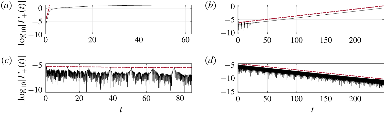
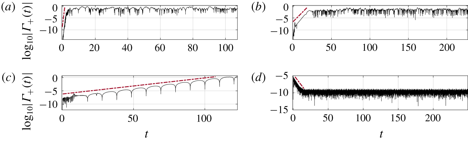
(Fixed–fixed) Examples of the log $_{10}$ of the total wake circulation versus time with (a)
 $(R_{1},T_{0})=(10^{-1.8},10^{-1.2})$, (b)
 $(R_{1},T_{0})=(10^{-0.2},10^{0.2})$, (c)
 $(R_{1},T_{0})=(10^{2},10^{1})$ and (d)
 $(R_{1},T_{0})=(10^{1},10^{3})$. The growth/decay rates are given by the slopes of the dot–dashed red lines. In all cases we set
 $R_{3}=1$, but the linear growth rates are independent of
 $R_{3}$ (we show the
 $R_{3}$ term to be cubic in deflection in (3.2a,b), and, therefore, negligible in the linear growth regime).

We use our nonlinear simulation to compute the stability threshold for membranes by applying the small transient perturbation (2.23) at the leading edge and observing exponential growth (followed by large-amplitude, nonlinear dynamics) or exponential decay in membrane deflection and wake circulation  $\unicode[STIX]{x1D6E4}_{+}(t)$. Examples are shown in figure 3. For the stability results presented in figures 3 and 4, we use (2.23) with
 $\unicode[STIX]{x1D70E}=10^{-6}$.
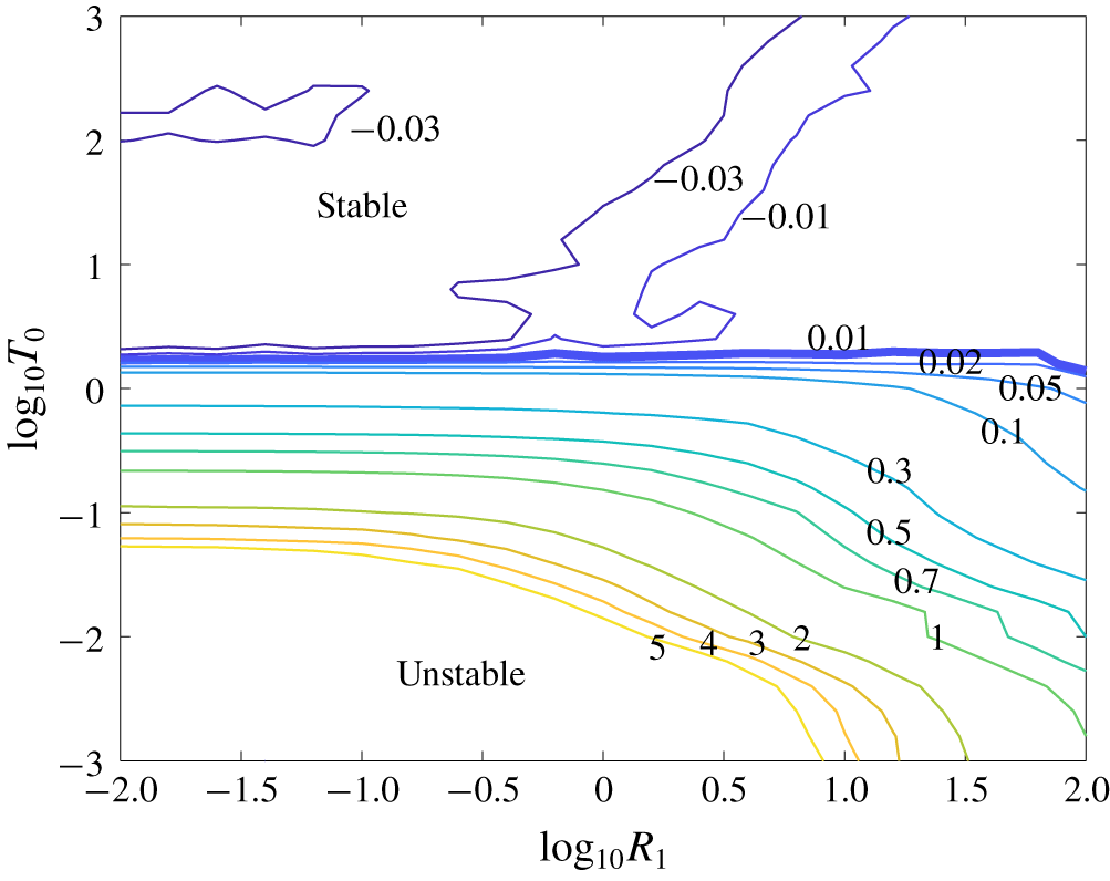
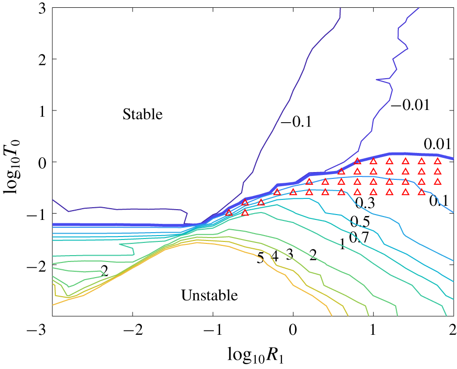
A contour plot of the exponential (base 10) growth and decay rates of wake circulation after a small transient perturbation, in the fixed–fixed case. The thicker line separates the stable and unstable cases.

We compute the growth and decay rates of the initial perturbation from data analogous to those in figure 3, on a fine grid of values in the  $R_{1}$–
 $T_{0}$ space spanning several orders of magnitude in each parameter. We show in figure 4 a contour plot of the growth/decay rates, i.e.
 $\unicode[STIX]{x1D6FD}$ in the early time interval, where
 $\unicode[STIX]{x1D6E4}_{+}(t)\approx K\,10^{\unicode[STIX]{x1D6FD}t}$ for some constant
 $K$. Values (well) above 5 occur in the lower-left corner, but are omitted for visual clarity. Above a critical pretension
 $T_{0}\approx 1.78$ the membranes are stable, with small transient deflections decaying to the flat state. Below the critical pretension, we have a divergence instability: small transient deflections grow exponentially at a rate that is purely real. Tiomkin & Raveh (Reference Tiomkin and Raveh2017) found a critical pretension of 1.73 in a slightly different model; unlike that study, we do not find evidence of neutral flutter or divergence with flutter in the fixed–fixed case at any
 $R_{1}$. The main differences are that our wake length grows from zero while that in Tiomkin & Raveh (Reference Tiomkin and Raveh2017) is infinite, and our model is a nonlinear, unsteady version of that in Tiomkin & Raveh (Reference Tiomkin and Raveh2017).
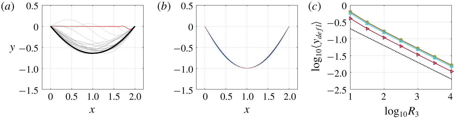
Fixed–fixed membrane shapes. (a) For  $R_{1}=10^{-0.5}$,
 $R_{3}=10^{1}$ and
 $T_{0}=10^{-3}$ the membrane shapes at
 $t=1$ (red),
 $1.5,2.5,3.5,4.5,\ldots ,16.5$ (light gray to black). (b) Steady membrane shapes at late times, with
 $y$ coordinates scaled by maximum deflection, for
 $R_{3}$ ranging from
 $10^{1}$ to
 $10^{4}$ and
 $T_{0}$ ranging from
 $10^{-3}$ to 1. (c) The maximum membrane deflection at steady state versus the stretching modulus
 $R_{3}$.

During the initial stages of the divergence instability, the membrane deflection grows from small amplitude without change of shape. Nonlinearities become important when the amplitude reaches order one, and the membrane shape evolves to its eventual steady state. For the large-amplitude analysis of fixed–fixed membranes that follows, the small transient perturbation (2.23) applied at the leading edge is used with  $\unicode[STIX]{x1D70E}=10^{-4}$. In figure 5(a) we show a sequence of membrane snapshots during the nonlinear dynamics. The earliest shape (red) is similar to those during the linear instability, with the largest deflection near the trailing edge. Subsequent shapes (ranging from light to dark gray and black) show the evolution to the eventual steady state. The final membrane shape is nearly fore-aft symmetrical, similar to those in Newman & Low (Reference Newman and Low1984), Tzezana & Breuer (Reference Tzezana and Breuer2019), Waldman & Breuer (Reference Waldman and Breuer2013, Reference Waldman and Breuer2017), Rojratsirikul, Wang & Gursul (Reference Rojratsirikul, Wang and Gursul2009) and Nardini et al. (Reference Nardini, Illingworth and Sandberg2018). These works also discuss membrane dynamics at non-zero angle of attack with applications to lift and thrust generation by membrane airfoils (possibly heaving and/or pitching (Jaworski & Gordnier Reference Jaworski and Gordnier2012)). Then vortices shed from the membrane’s leading edge provide an unsteady forcing, causing membrane oscillations even in the fixed–fixed case. However, the present work is focused on the problem of membrane flutter at zero angle of attack, for which leading edge vortex shedding should be less significant. As for most vortex panel methods (Katz & Plotkin Reference Katz and Plotkin2001), leading edge separation is difficult to represent in our model, so we focus on situations where trailing-edge vortex shedding is expected to be dominant, i.e. membranes at zero angle of attack with small-to-moderate deflections.
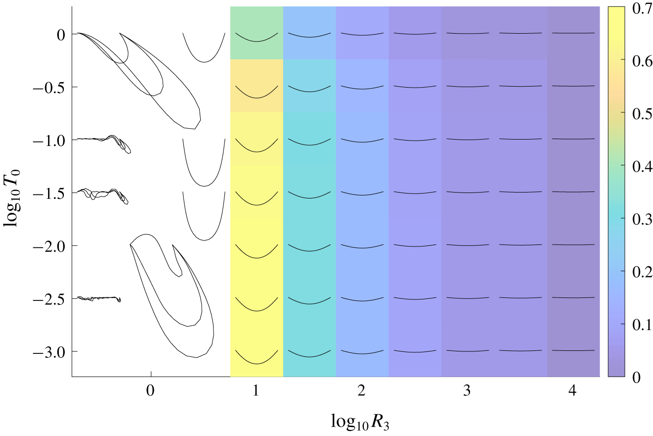
Membrane profiles in the fixed–fixed case, at steady state with moderate deflections (coloured background), or unphysically large or unsteady deflections (white background). In the unsteady cases a few snapshots at large times are shown. The colours show the deflection of the membrane (3.1). Here  $R_{1}=10^{-0.5},$ but the steady shapes are independent of
 $R_{1}$, the dimensionless mass.

In figure 6 we show the late-time membrane shapes across several decades of  $R_{3}$ and
 $T_{0}$. The shapes are all steady for
 $R_{3}>10^{0.5}$ (and, thus, independent of
 $R_{1}$ here, as the acceleration term in (2.8) is zero), but may oscillate chaotically for
 $R_{3}\leqslant 10^{0.5}$, in which case a few snapshots are shown at late times. In these cases, the deflections are so large as to violate the assumption that vortex shedding is confined to the trailing edge, so we do not consider them further. For
 $R_{3}>10^{0.5}$, the colours show the maximum membrane deflection. At a given
 $R_{3}$, the deflection increases slightly as
 $T_{0}$ decreases from the stability threshold to
 ${\approx}0.1$, then converges as
 $T_{0}$ decreases further, the
 $T_{0}$ term becoming insignificant in the membrane equation (2.8). At a given
 $T_{0}$, the deflection decreases with increasing
 $R_{3}$ as a power law. In figure 5(b) we show that the shapes are almost identical, however, when the amplitudes are normalized. In figure 5(c) we show that the deflection
 $\langle y_{defl}\rangle \sim 1/\sqrt{R_{3}}$ (for
 $R_{1}=10^{-0.5}$ here, but these values are independent of
 $R_{1}$).
We explain how the scaling  $\langle y_{defl}\rangle \sim 1/\sqrt{R_{3}}$ arises from the
 $y$-component of the membrane equation (2.8) with small deflections. We assume that
 $\unicode[STIX]{x2202}_{\unicode[STIX]{x1D6FC}}y\ll 1$ and
 $\unicode[STIX]{x2202}_{\unicode[STIX]{x1D6FC}}x\approx 1$. Then
 $\unicode[STIX]{x2202}_{\unicode[STIX]{x1D6FC}}s-1=\sqrt{(\unicode[STIX]{x2202}_{\unicode[STIX]{x1D6FC}}x)^{2}+(\unicode[STIX]{x2202}_{\unicode[STIX]{x1D6FC}}y)^{2}}-1\approx \unicode[STIX]{x2202}_{\unicode[STIX]{x1D6FC}}y^{2}/2$ and
 ${\hat{s}}_{y}\approx \unicode[STIX]{x2202}_{\unicode[STIX]{x1D6FC}}y$. With these approximations, the
 $y$-components of the
 $T_{0}$ and
 $R_{3}$ terms in (2.8) are linear and cubic in deflection, respectively:
 $$\begin{eqnarray}\unicode[STIX]{x2202}_{\unicode[STIX]{x1D6FC}}(T_{0}{\hat{s}}_{y})\approx T_{0}\unicode[STIX]{x2202}_{\unicode[STIX]{x1D6FC}\unicode[STIX]{x1D6FC}}y;\quad \unicode[STIX]{x2202}_{\unicode[STIX]{x1D6FC}}(R_{3}(\unicode[STIX]{x2202}_{\unicode[STIX]{x1D6FC}}s-1){\hat{s}}_{y})\approx R_{3}\unicode[STIX]{x2202}_{\unicode[STIX]{x1D6FC}}((\unicode[STIX]{x2202}_{\unicode[STIX]{x1D6FC}}y)^{3}/2).\end{eqnarray}$$
The  $R_{1}$ term (multiplying
 $\unicode[STIX]{x2202}_{tt}y$) is also linear in deflection (and zero here at steady state, but not for the oscillating membranes considered later). The pressure jump is linear in the bound vortex sheet strength because the left-hand side of (2.19)
 ${\approx}\unicode[STIX]{x2202}_{t}\unicode[STIX]{x1D6FE}+\unicode[STIX]{x2202}_{\unicode[STIX]{x1D6FC}}\unicode[STIX]{x1D6FE}$ with small deflections. The bound vortex sheet strength is linear in the deflection by the linearized version of (2.14),
 $$\begin{eqnarray}\unicode[STIX]{x2202}_{t}y(\unicode[STIX]{x1D6FC},t)\approx \frac{1}{2\unicode[STIX]{x03C0}}\;\unicode[STIX]{x2A0D}-_{-1}^{1}\frac{\unicode[STIX]{x1D6FE}(\unicode[STIX]{x1D6FC}^{\prime },t)}{x(\unicode[STIX]{x1D6FC},t)-x(\unicode[STIX]{x1D6FC}^{\prime },t)}\,\text{d}\unicode[STIX]{x1D6FC}^{\prime }-\frac{1}{2\unicode[STIX]{x03C0}}\!\int _{0}^{\unicode[STIX]{x1D6E4}_{+}(t)}\frac{x(\unicode[STIX]{x1D6FC},t)-x(\unicode[STIX]{x1D6E4}^{\prime },t)}{(x(\unicode[STIX]{x1D6FC},t)-x(\unicode[STIX]{x1D6E4}^{\prime },t))^{2}+\unicode[STIX]{x1D6FF}(\unicode[STIX]{x1D6E4}^{\prime },t)^{2}}\,\text{d}\unicode[STIX]{x1D6E4}^{\prime },\end{eqnarray}$$
in which the second integral consists of bound vorticity advected from the trailing edge, so it has the same dependence on deflection as the bound vorticity. Here, with small deflections, we have assumed that  $\unicode[STIX]{x2202}_{\unicode[STIX]{x1D6FC}}x\approx 1$, and then the linearization is the same as in Alben & Shelley (Reference Alben and Shelley2008). Without viscous stresses, horizontal membrane deformations arise only through nonlinear terms in the elastic and pressure forces associated with large deflections, so it is reasonable to neglect them, and this is consistent with the simulation results. Balancing the terms that are linear in deflection with the product of
 $R_{3}$ and a term that scales with deflection cubed gives
 $\langle y_{defl}\rangle \sim 1/\sqrt{R_{3}}$.
3.2 Fixed–free membranes
We now investigate membranes with the leading edge fixed and the trailing edge free to move vertically (with  $\unicode[STIX]{x2202}_{\unicode[STIX]{x1D6FC}}y=0$ there – an extra equation that determines
 $y(1,t)$, now an extra unknown). With the free end, the membrane has a wide range of unsteady dynamics with small and moderate amplitude, unlike in the fixed–fixed case, and similar in some respects to the fixed–free flag with bending rigidity (Alben & Shelley Reference Alben and Shelley2008).
(Fixed–free) Examples of the total wake circulation versus time for  $R_{3}=1$ on a log scale, with (a)
 $(R_{1},T_{0})=(10^{-3},10^{-2.8})$, (b)
 $(R_{1},T_{0})=(10^{-1.4},10^{-1.4})$, (c)
 $(R_{1},T_{0})=(10^{1},10^{-0.2})$ and (d)
 $(R_{1},T_{0})=(10^{-0.8},10^{2.2})$. The slopes of the dot–dashed red lines give the growth/decay rates. Recall that
 $R_{1}$ is the dimensionless membrane mass,
 $T_{0}$ is the dimensionless pretension and
 $R_{3}$ is the dimensionless stretching modulus.

In figure 7 we show examples of the growth of wake circulation in time after small transient perturbations, analogous to figure 3. As before, for the analysis of the small-amplitude dynamics, we use (2.23) with  $\unicode[STIX]{x1D70E}=10^{-6}$. The main novelty is panel (c), an example of divergence with flutter – shown by the regularly spaced vertical asymptotes in the logarithm of wake circulation, corresponding to an oscillatory component – exponential growth with a complex growth rate.
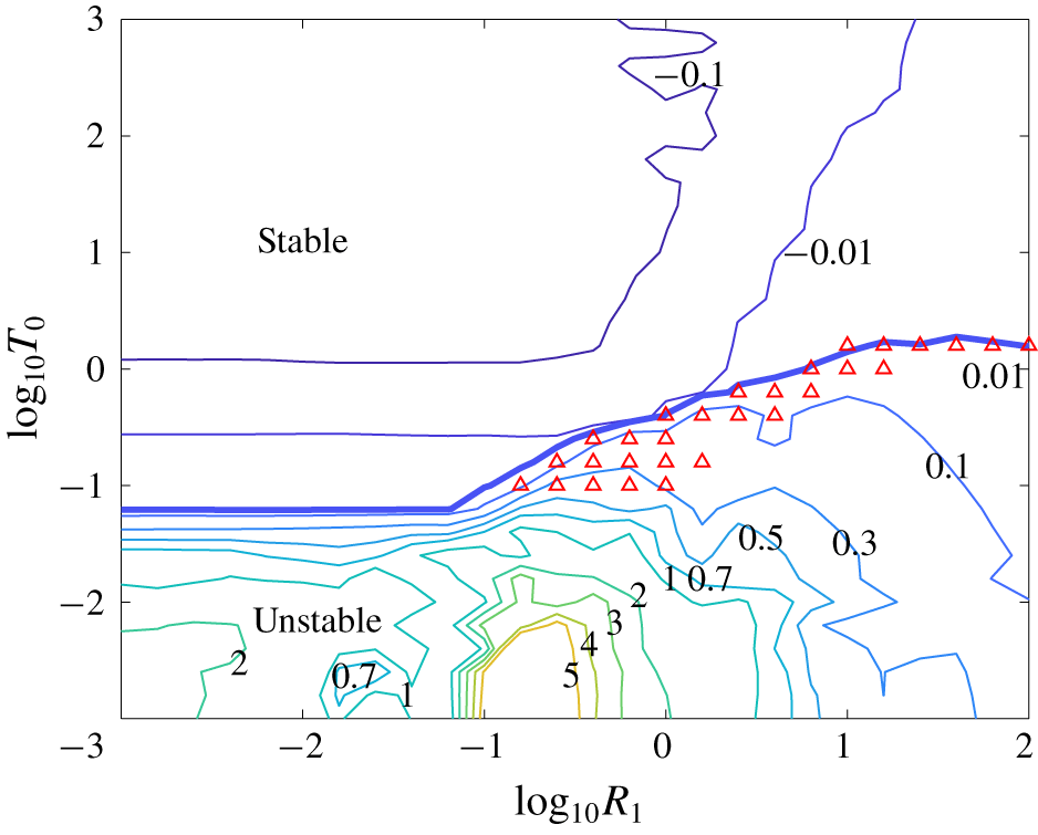
A contour plot of the exponential (base 10) growth and decay rates of wake circulation after a small transient perturbation, in the fixed–free case. The thicker line separates the regions where the membranes are stable and unstable. Growth rates (well) above 5 occur at the lower left but are omitted for visual clarity.

We show in figure 8 a contour plot of the growth/decay rates and stability boundary in  $R_{1}$–
 $T_{0}$ space, analogous to figure 4. Notable differences are that the stability boundary now varies with
 $R_{1}$. The critical pretension is close to that in figure 4 at the largest
 $R_{1}$, but decreases as
 $R_{1}$ decreases, and eventually reaches a lower plateau at
 $R_{1}\ll 1$. The red triangles in figure 8 show cases like figure 7(c), membranes that become unstable through flutter and divergence.
The membranes in the unstable region of figure 8 eventually reach large amplitudes, where nonlinearities (e.g. the  $R_{3}$ term) determine the eventual steady-state motion. With fixed–free boundary conditions, oscillatory motions are typical, unlike for the fixed–fixed case. As for the fixed–fixed case, unrealistically large deflections occur for
 $R_{3}\leqslant 1$, so we focus on
 $R_{3}\gtrsim 1$.
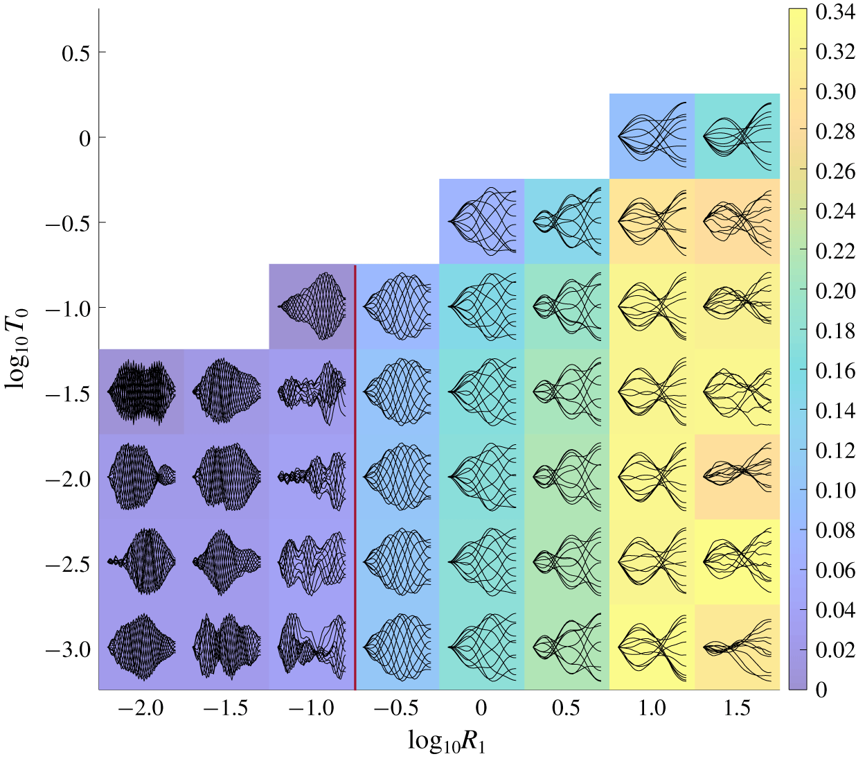
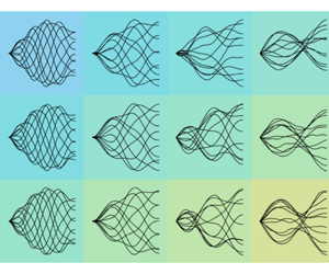
(Fixed–free) Snapshots of large-amplitude membrane motions in the unstable region of  $R_{1}$–
 $T_{0}$ space for fixed
 $R_{3}=10^{1.5}$. Colours denote
 $\log _{10}$ of the average deflection defined by (3.1). At each (
 $R_{1}$,
 $T_{0}$) value, the set of snapshots is normalized by the maximum deflection of the snapshots to show the deformation modes more clearly and scaled to fit within a coloured rectangle at the (
 $R_{1}$,
 $T_{0}$) value.

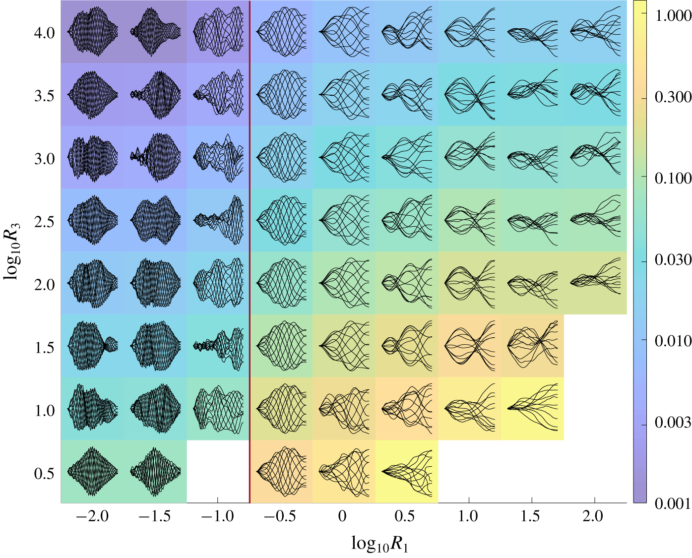
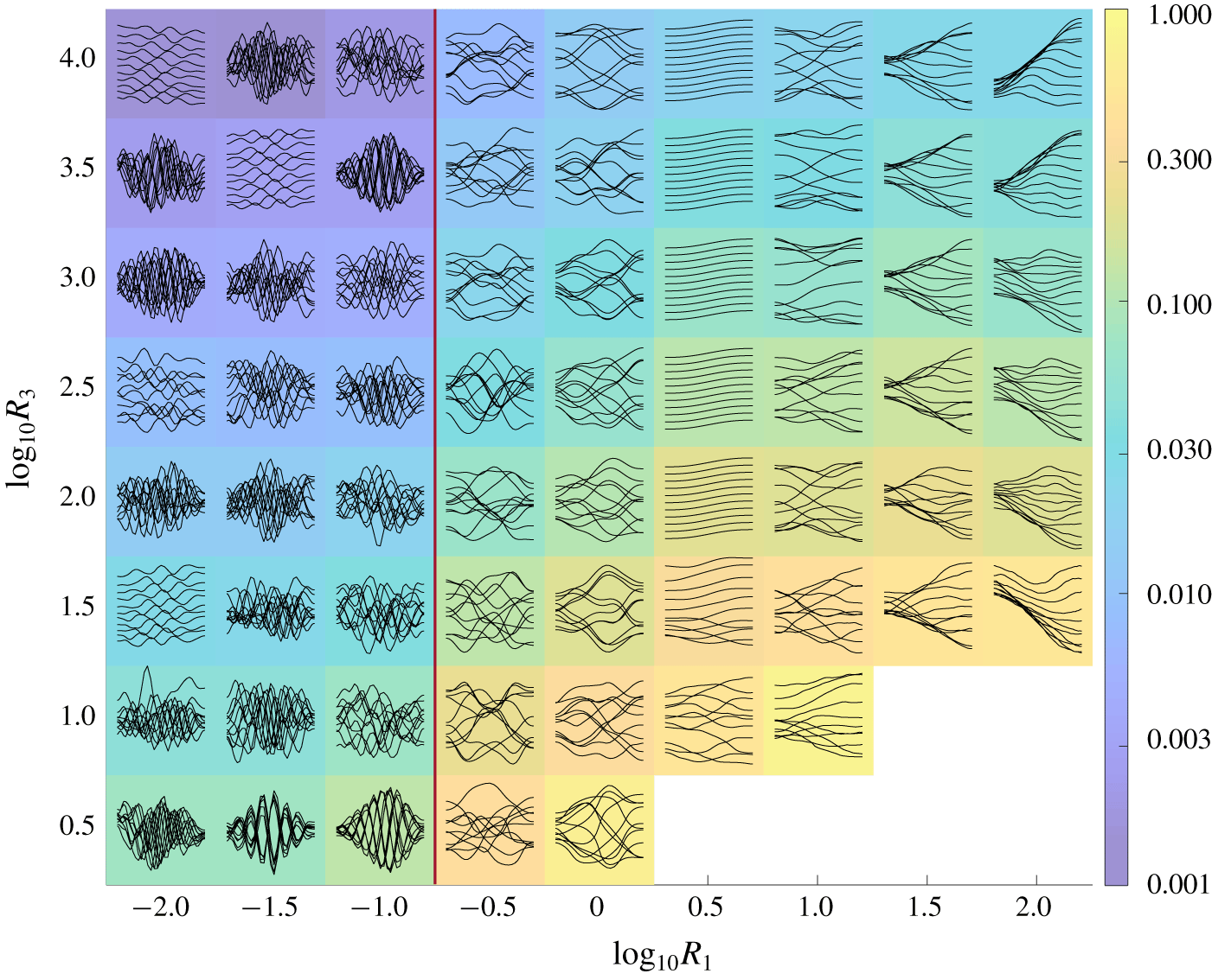
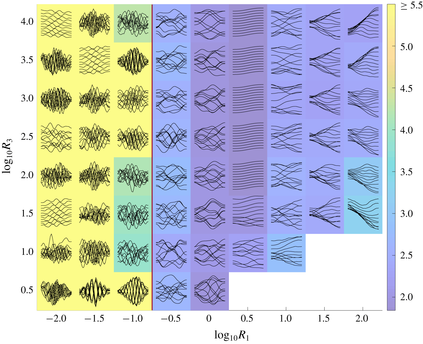
(Fixed–free) Snapshots of large-amplitude membrane motions in  $R_{1}$–
 $R_{3}$ space for fixed
 $T_{0}=10^{-2}$. Colours denote
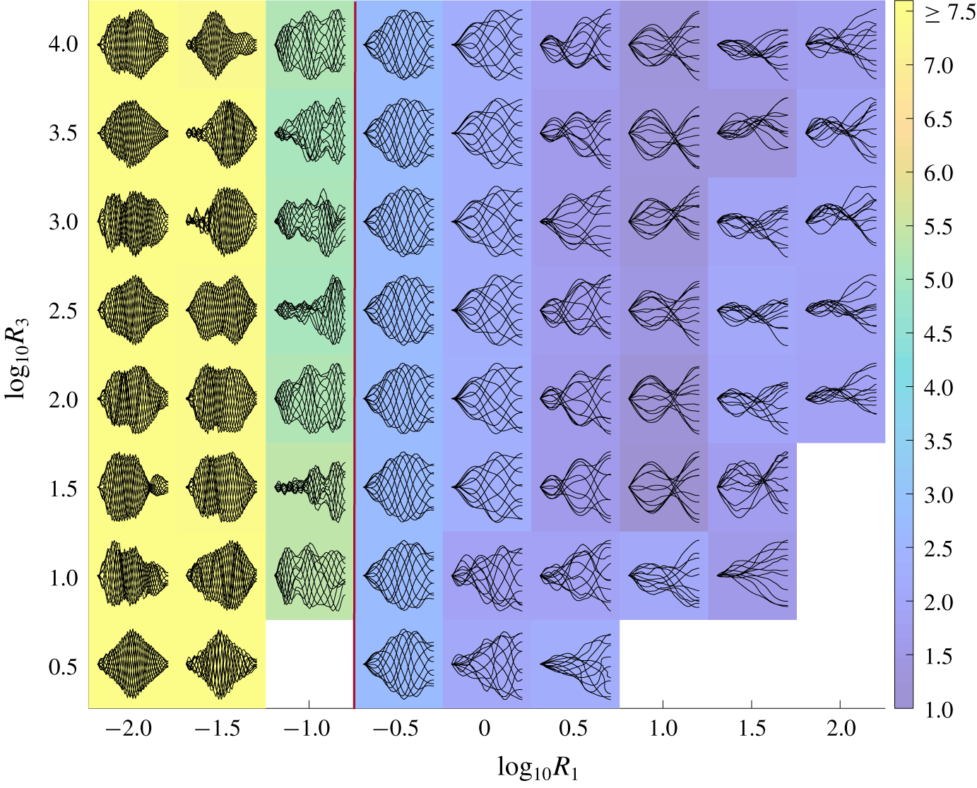
 $\log _{10}$ of the average deflection defined by (3.1). To the right of the vertical red dividing line the membrane motions are nearly periodic, but to the left of the red line the membrane oscillations are chaotic. At each (
 $R_{1}$,
 $R_{3}$) value, the set of snapshots is scaled to fit within a coloured rectangle at the (
 $R_{1}$,
 $R_{3}$) value and normalized by the maximum deflection of the snapshots to show the motions more clearly.

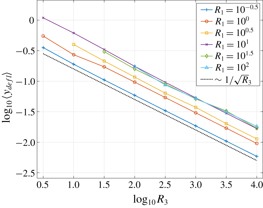
(Fixed–free.) Time-averaged deflections of the membranes (defined by (3.1)) versus  $R_{3}$ for various
 $R_{1}$ and fixed
 $T_{0}=10^{-2}$. The black dashed line indicates the scaling
 $1/\sqrt{R_{3}}$.

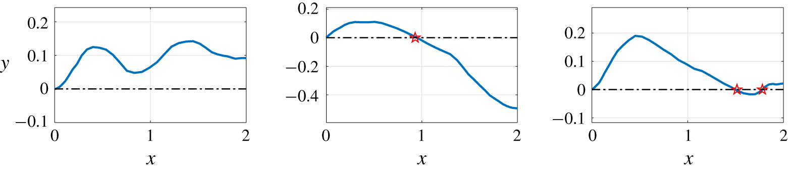
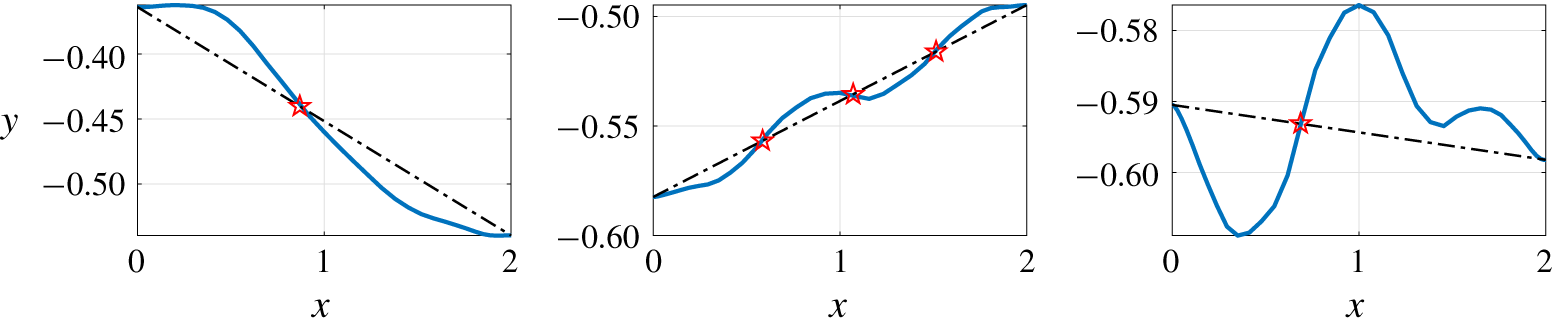
Examples of where zero crossings (red stars) are counted for model membranes (blue solid lines). Note that the leading edge of the membrane is not included as a zero crossing.

(Fixed–free.) Colours denote the time-averaged number of zero crossings for membrane flutter in the  $R_{1}$–
 $R_{3}$ parameter space for fixed
 $T_{0}=10^{-2}$. In the lower-right corner and at
 $(R_{1},R_{3})=(10^{-1},10^{0.5})$, snapshots are omitted because steady-state membrane motions were not obtained. Note that
 $R_{1}$ is the dimensionless membrane mass,
 $T_{0}$ is the dimensionless pretension and
 $R_{3}$ is the dimensionless stretching modulus. At each (
 $R_{1}$,
 $R_{3}$) value the set of snapshots is normalized by the maximum deflection of the snapshots to show the motions more clearly.

Now we study the large-amplitude dynamics and we use  $\unicode[STIX]{x1D70E}=10^{-4}$ in (2.23). In figure 9 we show typical membrane snapshots in the unstable region of
 $R_{1}$–
 $T_{0}$ space from figure 8. At each (
 $R_{1}$,
 $T_{0}$) value, the set of snapshots is normalized by the maximum deflection of the snapshots to show the motions more clearly and scaled to fit within a coloured rectangle at the (
 $R_{1}$,
 $T_{0}$) value. Each snapshot has the corresponding
 $R_{1}$ value at its horizontal midpoint, and the
 $T_{0}$ value at its leading edge. Here
 $R_{3}$ is fixed at
 $10^{1.5}$, a value giving moderately large deflections for the steady-state motion. The colours denote the average deflection of the membrane (3.1).
The motions in figure 9 have the largest deflection amplitudes and smallest spatial frequency components at the largest  $R_{1}(10^{1.5})$. Intuitively speaking, large
 $R_{1}$ (membrane inertia) allows the membrane to maintain its momentum for longer times against restoring fluid forces, and obtain larger deflections before reversing direction. The same has been observed for flutter with bending rigidity (Connell & Yue Reference Connell and Yue2007; Alben & Shelley Reference Alben and Shelley2008). As
 $R_{1}$ decreases, the membrane deflection amplitudes progressively decrease and spatial frequencies increase until the motions become difficult to resolve numerically (to the left of the red vertical line). In this region, we find chaotic membrane oscillations with very small amplitudes and high spatial frequencies that become independent of
 $R_{1}$. When the number of points on the membrane is increased from
 $40$ (here) to 80, 160 and 200, the membranes with
 $R_{1}\leqslant 10^{-1}$ still oscillate chaotically but with even higher spatial frequency components, while those with
 $R_{1}\geqslant 10^{-0.5}$ do not change significantly. Although the motions to the left of the red line are not converged with respect to the spatial grid, we retain their snapshots in figure 9 to indicate the behavior of the simulations. We find quasi-periodic motions in a finite band of
 $R_{1}$ values between
 $10^{-0.5}$ and
 $10^{0.5}$. Above and below this range, the motions become more irregular and chaotic, and more up–down asymmetrical at large
 $R_{1}$. The membrane motion depends weakly on
 $T_{0}$ except near the stability boundary (at the largest
 $T_{0}$ shown). At smaller
 $T_{0}$, the pretension does not affect the dynamics because it is negligible compared to the
 $R_{3}$ (stretching) term.
Next we look at the same quantities in a different two-dimensional slice through  $R_{1}$–
 $T_{0}$–
 $R_{3}$ space. We fix
 $T_{0}=10^{-2}$ and in figure 10 show the membrane motions across
 $R_{1}$ and
 $R_{3}$. In the lower-right corner and at
 $(R_{1},R_{3})=(10^{-1},10^{0.5})$, snapshots are omitted because steady-state membrane motions were not obtained. We find that
 $R_{3}$ mainly affects the amplitudes of the snapshots, but not their shapes, particularly for the periodic motions with
 $R_{1}=10^{-0.5}$. The shapes do change noticeably for the more irregular and chaotic motions, which are sensitive to small changes in parameters, and near the smallest stretching modulus where steady-state motions occur,
 $R_{3}\approx 10^{0.5}$.
We find that membranes with  $R_{1}=10^{-0.5}$–
 $10^{0.5}$ move almost like traveling waves: their peaks and troughs translate downstream in forward time. Some of those with larger
 $R_{1}$ (
 $10^{1}$ and
 $10^{1.5}$) move approximately like standing waves, with a node and an antinode at certain locations. Similar dynamics have been found for fixed–fixed membranes perturbed by vortices shed from the leading edge (Song et al. Reference Song, Tian, Israeli, Galvao, Bishop, Swartz and Breuer2008; Gordnier Reference Gordnier2009; Timpe et al. Reference Timpe, Zhang, Hubner and Ukeiley2013).
We show how the time-averaged deflection depends on  $R_{3}$ at several fixed values of
 $R_{1}$ in figure 11. The plots follow the same
 $1/\sqrt{R_{3}}$ dependence at large
 $R_{3}$ as in the fixed–fixed case and for the same reason (explained in § 3.1).
In figure 10 we show the typical membrane motions at various  $R_{1}$ and
 $R_{3}$ at fixed
 $T_{0}$ (and the phenomena are similar at other
 $T_{0}$ that yield flutter). We now quantify the membrane shapes in terms of the time-averaged number of ‘zero crossings’ – the number of times the membrane crosses
 $y=0$. This is one way to measure the ‘waviness’ of a shape which is not sinusoidal (so the wavelength is not well defined) (Alben & Shelley Reference Alben and Shelley2008; Alben Reference Alben2015). In figure 12 we show examples of shapes with zero, one, and two zero-crossings, respectively.
We have already mentioned the trend to higher spatial frequency components with decreasing  $R_{1}$. In figure 13 we quantify this relationship by showing the average number of zero crossings for the same snapshots in figure 10 (where the deflection amplitude was plotted). Decreasing
 $R_{1}$ from the largest value (
 $10^{2}$), the average number of zero crossings actually decreases slightly to about 1 near
 $10^{1}$, and then increases with further decreases in
 $R_{1}$ as the motions become more periodic and then more irregular at yet smaller
 $R_{1},$ where the motions are not fully resolved spatially.
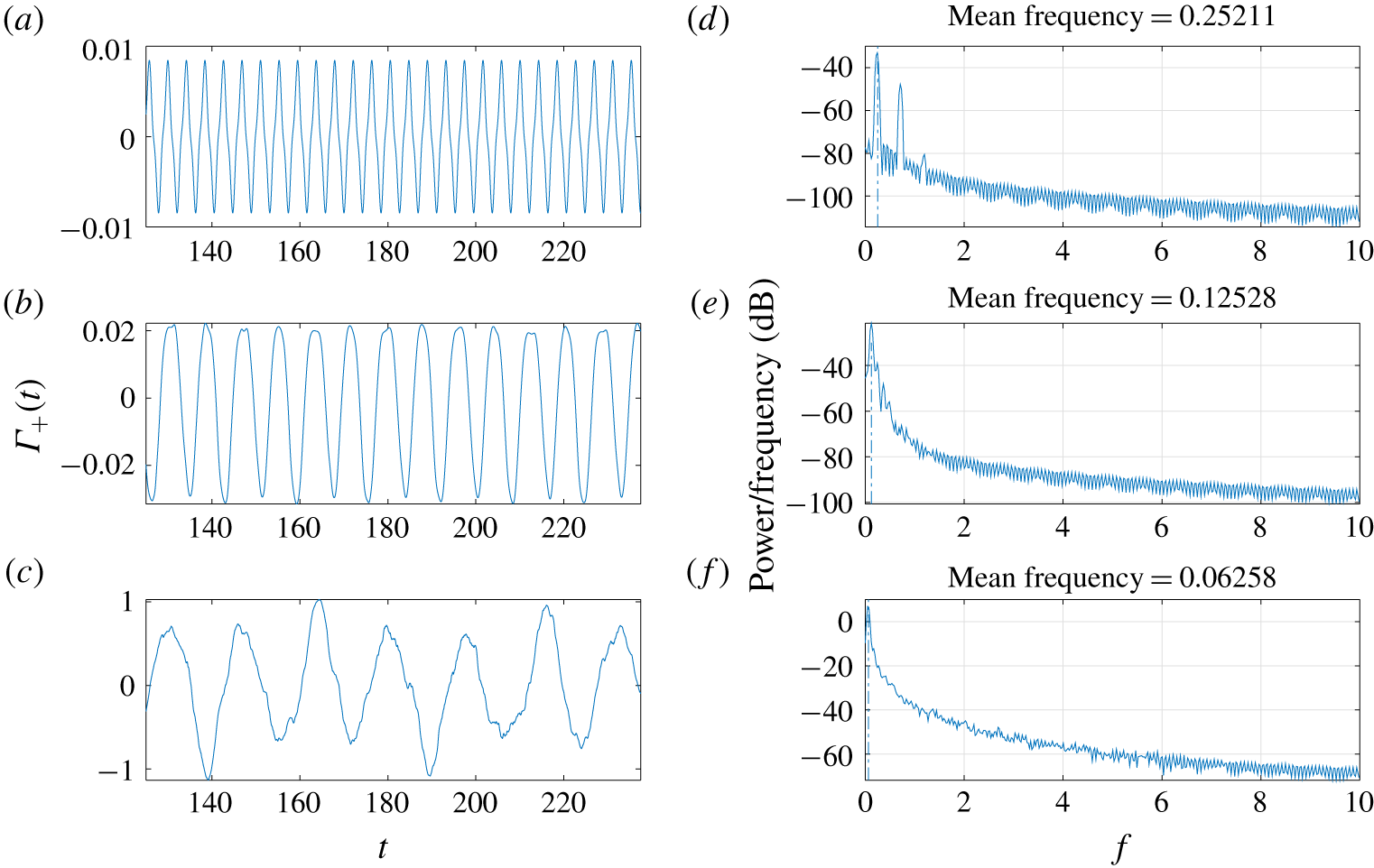
The temporal dynamics corresponding to these motions are quantified by computing the power spectra of time series of the total wake circulation,  $\unicode[STIX]{x1D6E4}_{+}(t)$. In figure 14 we show examples of the time series of
 $\unicode[STIX]{x1D6E4}_{+}(t)$ that correspond to the different types of power spectra. Panel (a) shows an example with a periodic motion at
 $R_{1}=10^{-0.5}$. The corresponding
 $\unicode[STIX]{x1D6E4}_{+}(t)$ is periodic though not sinusoidal, resulting in a sequence of sharp peaks in the power spectrum. Panel (b) shows a less periodic response at larger
 $R_{1}$, still dominated by a single frequency but with clear variations from one cycle to the next. In panel (c) at still larger
 $R_{1}$, the trend toward aperiodicity continues. Nonetheless, the time series (left) shows peaks with a somewhat regular spacing. The corresponding power series (right) has a single peak close to zero frequency and a gradual decay in the power spectrum at higher frequencies, typical of chaotic dynamics.
(Fixed–free.) A portion of the time series of total wake circulation  $\unicode[STIX]{x1D6E4}_{+}(t)$ (a–c) and corresponding power spectra (d–f) for membranes with increasing mass density
 $R_{1}$ from top to bottom: (a,d)
 $(R_{1},R_{3})=(10^{-0.5},10^{2})$, (b,e)
 $(R_{1},R_{3})=(10^{0.5},10^{3.5})$ and (c,f)
 $(R_{1},R_{3})=(10^{1.5},10^{1.5})$. In all cases
 $T_{0}=10^{-2}$.

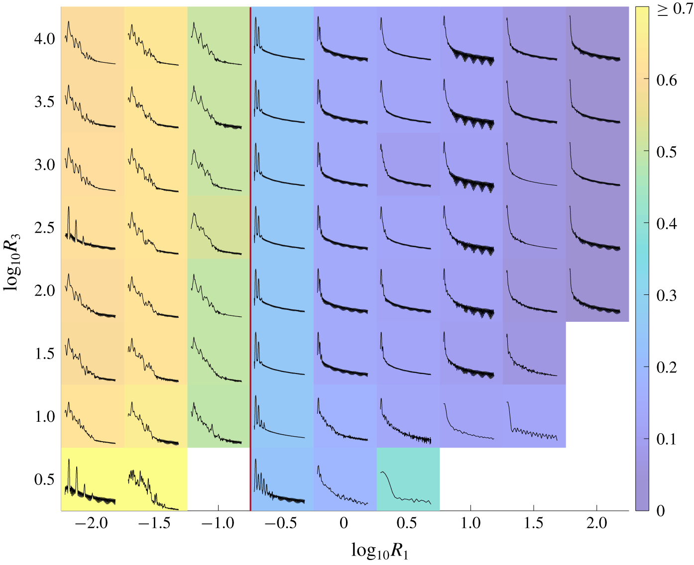
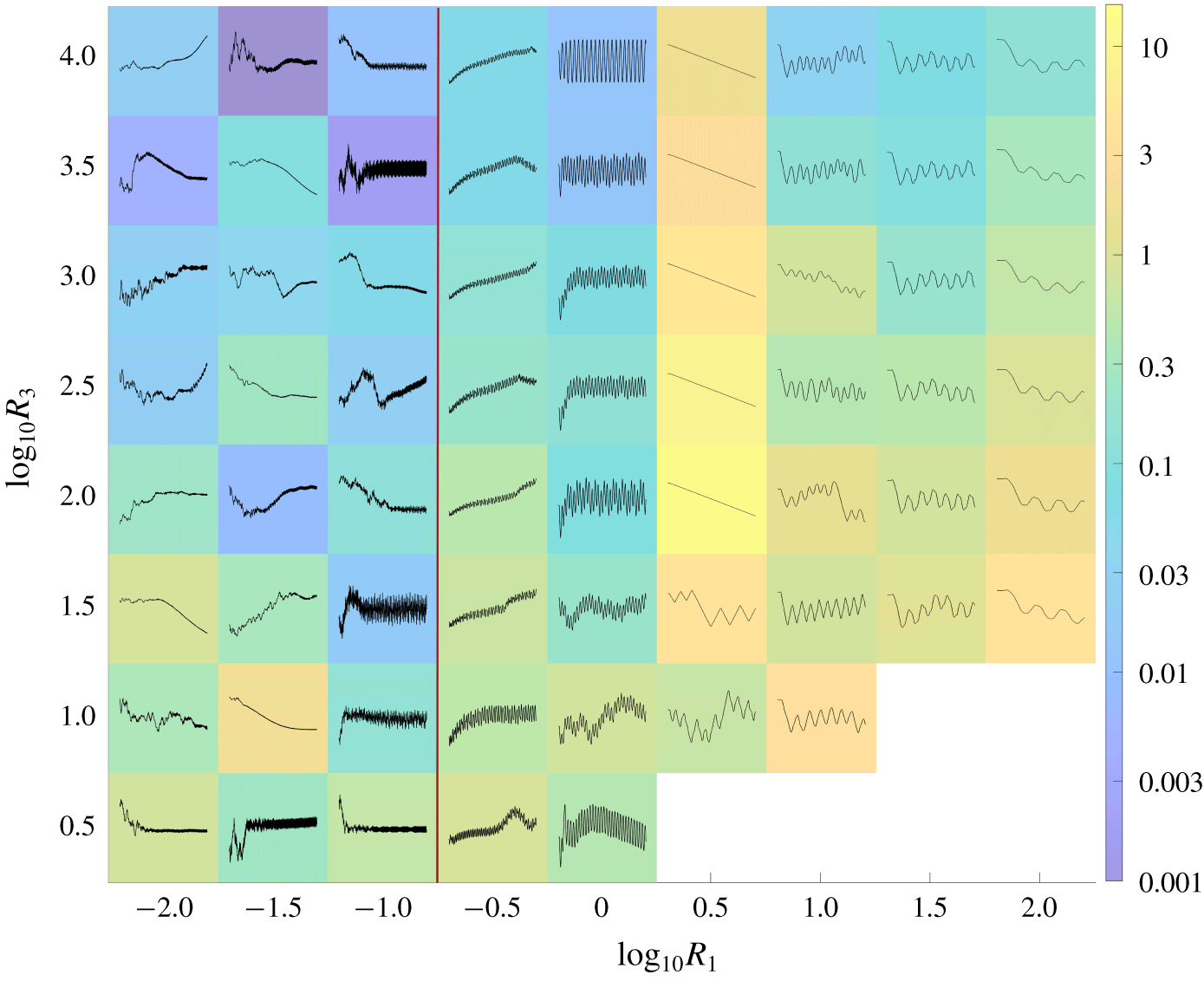
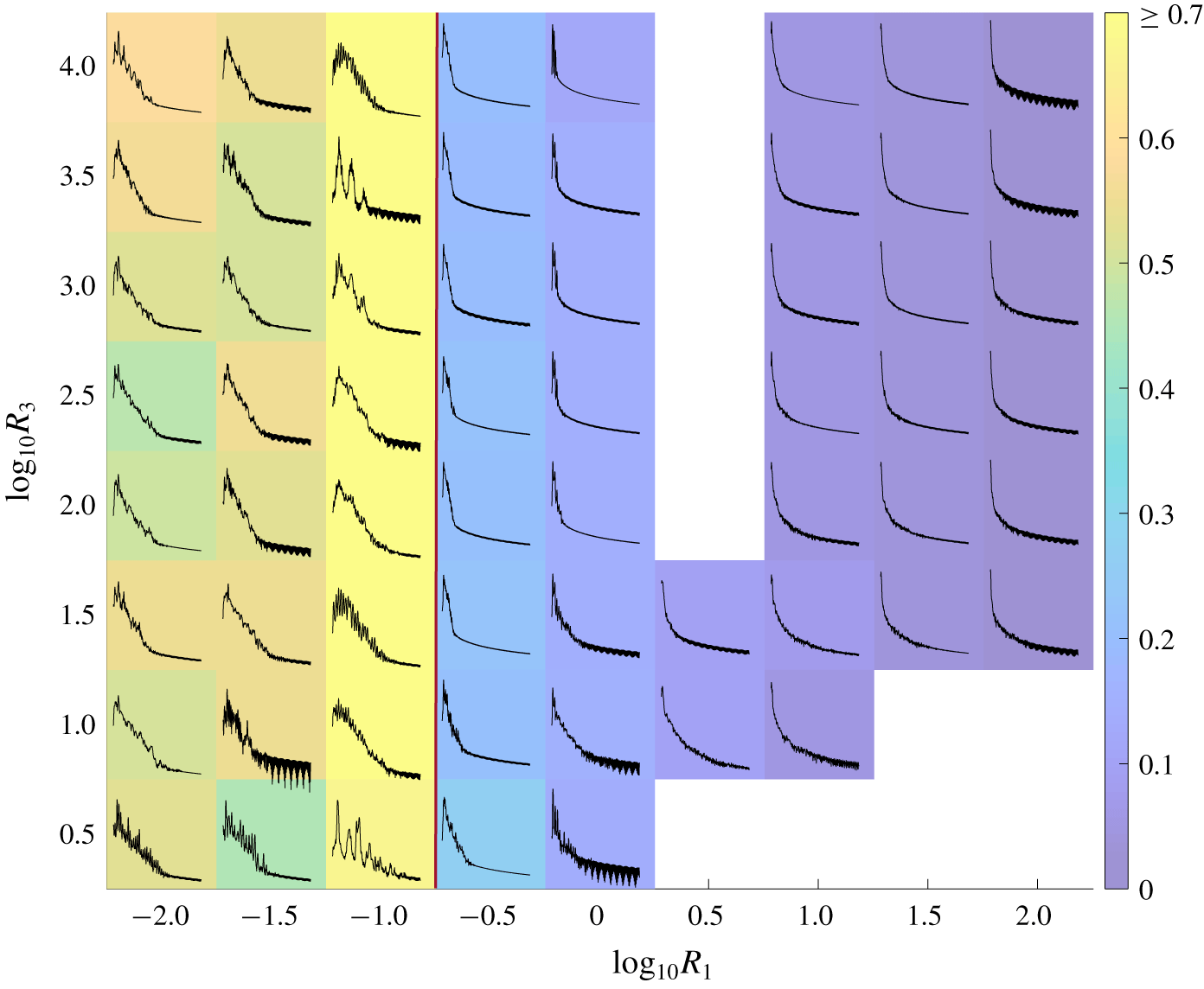
Colours denote the mean frequencies of large-amplitude motions in the fixed–free case for various  $R_{1}$ and
 $R_{3}$, all with
 $T_{0}=10^{-2}$. The corresponding power spectra for each membrane are plotted in black. In the lower-right corner and at
 $(R_{1},R_{3})=(10^{-1},10^{0.5})$, power spectra are omitted because steady-state membrane motions were not obtained. Each power spectrum is a plot of power density (per unit frequency) versus frequency as in the right-hand side panels of figure 14. The axis scales are omitted due to space constraints but our focus here is on the qualitative features only.

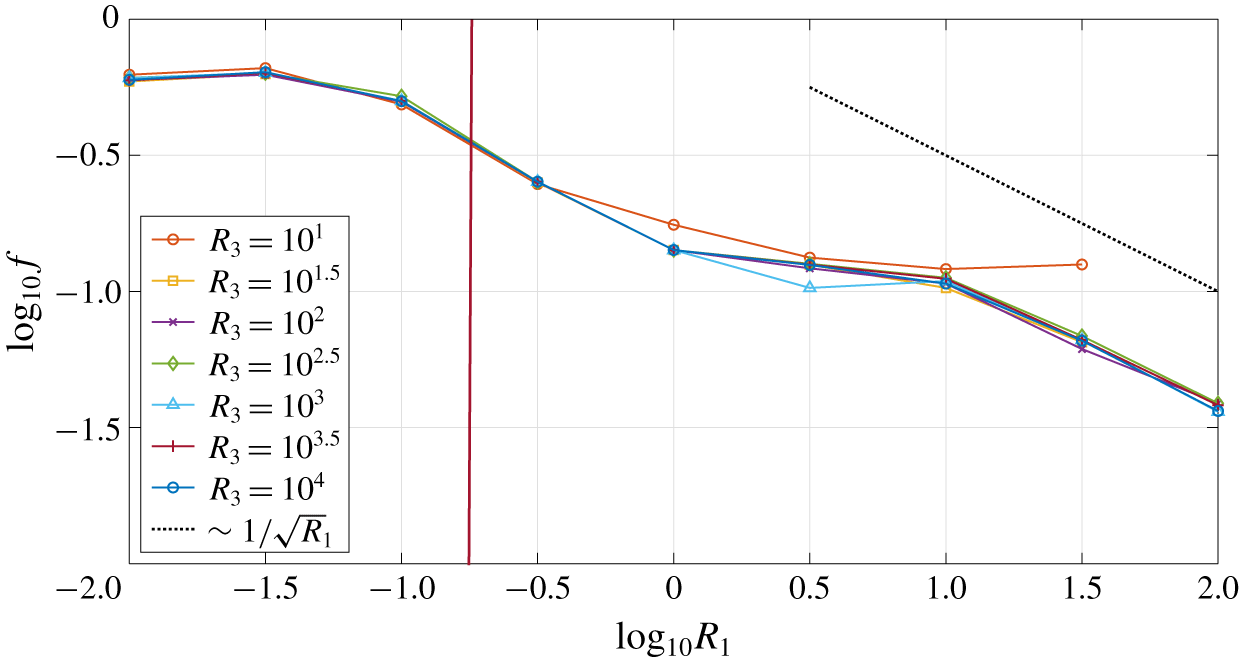
(Fixed–free) Plots of the mean frequency  $\log _{10}f$ versus mass density
 $\log _{10}R_{1}$ with various
 $R_{3}$ and fixed
 $T_{0}=10^{-2}$. The black dashed line shows the scaling
 $1/\sqrt{R_{1}}$.

In figure 15 we show these spectra, computed using Welch’s method (Welch Reference Welch1967), across  $R_{1}$–
 $R_{3}$ space with
 $T_{0}=10^{-2}$. The colours denote the mean frequencies, i.e. the first moments of the power spectra, normalized by total power. As
 $R_{1}$ increases from 10
 $^{-0.5}$ to 10
 $^{2}$ and the dynamics change from periodic to chaotic, the power spectra change as described in the previous figure, with little dependence on
 $R_{3}$ except at the lowest values. The mean frequencies decrease by about a factor of five. Thus, there is a strong correlation between the number of zero crossings (or flutter mode) and oscillation frequency, as has been seen previously in flag flutter problems (Shelley et al. Reference Shelley, Vandenberghe and Zhang2005; Eloy et al. Reference Eloy, Souilliez and Schouveiler2007; Alben & Shelley Reference Alben and Shelley2008; Alben Reference Alben2015). The two are in linear proportion for the modes of the linear wave equation for a membrane in a vacuum (Graff Reference Graff1975; Farlow Reference Farlow1993). The power spectra to the left of the red line (for motions which are not converged with respect to grid spacing) show higher frequencies and a broadband response, reflecting chaotic dynamics.
In figure 16 we show more quantitatively how the mean frequency varies with parameters. There is very little dependence on  $R_{3}$ except near the smallest
 $R_{3},$ where stable motions can be computed,
 ${\approx}10^{1}$. There is a steady decrease from
 $R_{1}=10^{-1}$ to
 $10^{0}$ followed by a small plateau for
 $10^{0}\leqslant R_{1}\leqslant 10^{1}$, and another decrease within
 $10^{1}\leqslant R_{1}\leqslant 10^{2}$. The trend at the largest
 $R_{1}$ is well approximated by
 $f\sim 1/\sqrt{R_{1}}$ (admittedly over a short range of
 $R_{1}$), except at the two smallest
 $R_{3}$ values. This scaling arises when one approximates the normal component of the membrane equation (2.8) by its
 $y$-component, and chooses a characteristic time scale
 $t_{0}$ so that
 $R_{1}\unicode[STIX]{x2202}_{tt}y$ balances other terms that depend on
 $y$ but not its time derivatives (i.e. the
 $R_{3}$ and
 $T_{0}$ terms and some of the fluid pressure terms). At large
 $R_{1}$,
 $R_{1}\unicode[STIX]{x2202}_{tt}y$ is comparable to the other terms when
 $R_{1}/t_{0}^{2}\sim 1$ or
 $t_{0}\sim \sqrt{R_{1}}$, giving a typical frequency
 $f_{0}\sim 1/\sqrt{R_{1}}$.
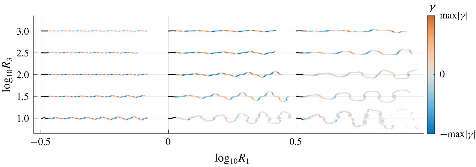
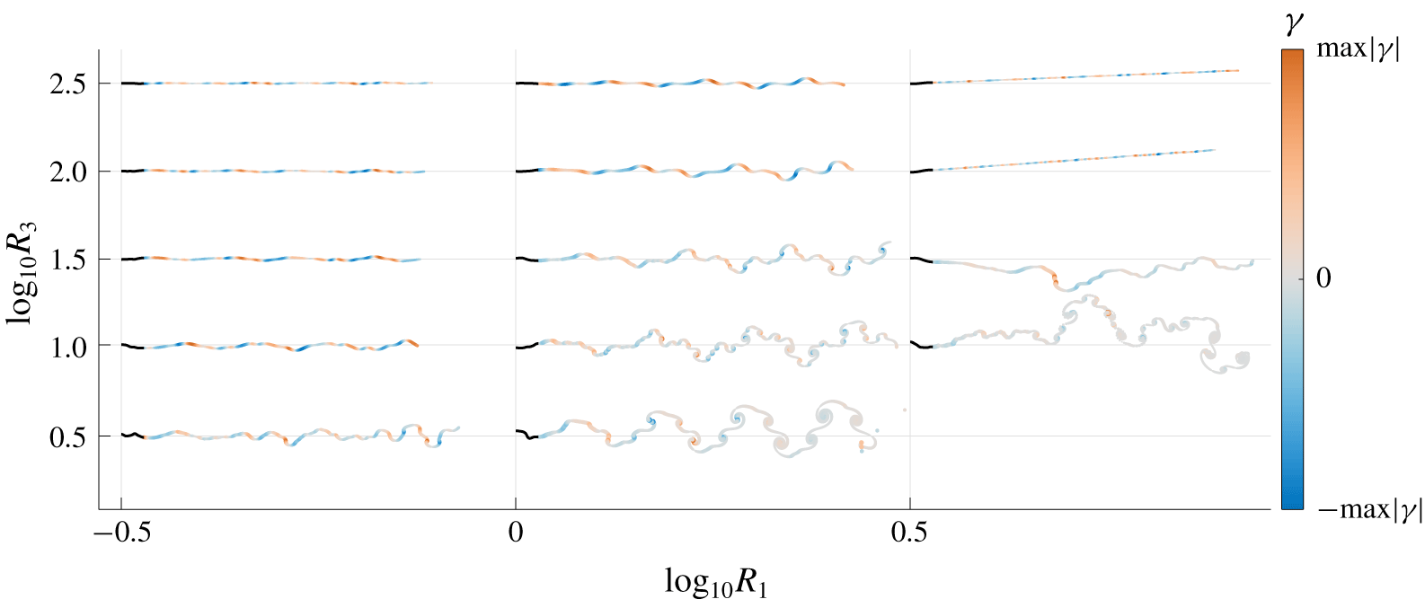
(Fixed–free) Snapshots of the membrane motion (in black) and the vortex wake in a portion of the  $R_{1}$–
 $R_{3}$ parameter space for fixed
 $T_{0}=10^{-2}$. In each case the
 $(R_{1},R_{3})$ values are marked at the left endpoint of the membrane. The wake is colour-coded according to the vortex sheet strength at the last time step. It is also thickness-coded according to
 $15|\unicode[STIX]{x1D6FE}|^{1/3}$. Counterclockwise rotating vortices are shown in orange and clockwise rotating vortices in blue. For example, for
 $(R_{1},R_{3})=(10^{-0.5},10^{3}),$ we have
 $\max |\unicode[STIX]{x1D6FE}|=0.0041$ and for
 $(R_{1},R_{3})=(10^{0.5},10^{1}),$ we have
 $\max |\unicode[STIX]{x1D6FE}|=1.9$.

We have mainly focused on the membrane dynamics, but we conclude this section by briefly considering the vortex sheet wake dynamics. In figure 17 we show snapshots of vortex wakes in a small portion of  $R_{1}$–
 $R_{3}$ space, where the membranes’ motions transition from small to large amplitudes. At smaller amplitudes (top and left), the wakes are mostly flat (despite the complexity of the corresponding membrane snapshots, shown in figure 10) and have periodic undulations, as the membrane motions are approximately periodic at these parameters. Here the vorticity is weak, so there is little vortex wake roll-up before the wake is advected many body lengths downstream by the background flow. With smaller membrane deflections, we observe two pairs of oppositely signed vortices per flapping period (
 $R_{1}=10^{-0.5}$ with
 $R_{3}=10^{1}$–
 $10^{3}$, and
 $R_{1}=10^{0}$ with
 $R_{3}=10^{1.5}$–
 $10^{3}$), akin to a 2P wake (Williamson & Roshko Reference Williamson and Roshko1988). At larger deflections, there is more roll-up and the wake resembles a von Kármán vortex street in some cases (
 $R_{1}=10^{0.5}$ with
 $R_{3}=10^{1.5}$–
 $10^{2.5}$), or a less regular wake with many spirals per flapping period (bottom right,
 $R_{1}=10^{0}$–
 $10^{0.5}$ with
 $R_{3}=10^{1}$). In general, the wake is spatially periodic to the extent that the membrane motion is temporally periodic. The more irregular wakes reflect the greater aperiodicity of the membrane motion at large amplitudes.
3.3 Free–free membranes
We have seen that changing the trailing edge boundary condition from fixed to free dramatically changes the membrane dynamics, from static deflections with a single maximum to a wide range of oscillatory modes that have some commonalities with flapping plates and flags (Shelley & Zhang Reference Shelley and Zhang2011). Therefore, it is natural to consider the effect of making both ends free, and determine if the membrane dynamics undergo further dramatic changes. Computationally, the method is the same as before, but the system of unknowns now includes the values of  $y$ at both endpoints, corresponding to the two equations
 $\unicode[STIX]{x2202}_{\unicode[STIX]{x1D6FC}}y(-1,t)=\unicode[STIX]{x2202}_{\unicode[STIX]{x1D6FC}}y(1,t)=0$.
A contour plot of the exponential (base 10) growth and decay rates of wake circulation after a small transient perturbation, in the free–free case. The thicker line separates the stable membranes from the unstable ones.

The contour plot of growth/decay rates of the initial perturbation ((2.24) with  $\unicode[STIX]{x1D70E}=10^{-3}$) is shown in figure 18. It is similar to that in the fixed–free case (figure 8), particularly in the location of the stability boundary and the contours in the stable region. In the unstable region, the growth rates are significantly smaller and there are slight differences in where divergence with flutter occurs (red triangles).
We now consider the large-amplitude membrane motions in  $R_{1}$–
 $R_{3}$ space with
 $T_{0}$ fixed at
 $10^{-2}$, the free–free analog of figure 10. In figure 19 we show the motions superposed on a colour field that labels the time-averaged membrane deflections (3.1). The membrane is now free to translate in the
 $y$-direction, which leads to additional complexities in the motions. As in the fixed–free case (figure 10), increasing
 $R_{3}$ decreases the deflections of the snapshots without significantly changing the qualitative features of their shapes. Decreasing
 $R_{1}$ generally decreases the deflections also, except near the largest
 $R_{1}$. The membranes mostly oscillate within a fixed vertical region, except at
 $R_{1}=10^{0.5}$, where the membranes mostly translate steadily in
 $y$, and with a steady shape. The membranes are somewhat straighter than in the fixed–free case, possibly because their translational freedom allows them to align more closely with the oncoming flow. As
 $R_{1}$ decreases below
 $10^{0.5}$, the membranes develop sharper curvatures until they again become difficult to resolve numerically at and below
 $10^{-1}$. To the left of the red dividing line, increasing the number of points on the membrane leads to similarly complex oscillatory motions with somewhat sharper curvatures in most cases.
Membrane snapshots in the free–free case superposed on colours labeling the time-averaged deflection for each ( $R_{1},R_{3}$) pair with
 $T_{0}=10^{-2}$ defined by (3.1). Recall that
 $R_{1}$ is the dimensionless membrane mass,
 $T_{0}$ is the dimensionless pretension and
 $R_{3}$ is the dimensionless stretching modulus. At each (
 $R_{1}$,
 $R_{3}$) value, the set of snapshots is scaled to fit within a coloured rectangle at the (
 $R_{1}$,
 $R_{3}$) value and normalized by the maximum deflection of the snapshots to show the motions more clearly.

To show the net translational motions of the membranes, we plot in figure 20 the  $y$ coordinates of the membranes’ midpoints over time. The colour denotes the net
 $y$ displacement up to
 $t=250$. At
 $R_{1}=10^{2}$, the membranes’ translational motions are generally oscillatory with long time intervals between changes in vertical direction. Decreasing
 $R_{1}$ generally decreases the lengths of these intervals, corresponding to higher frequency translational motions. At
 $R_{1}=10^{0.5}$, the membranes translate steadily (with occasional changes in direction, at
 $R_{3}=10^{1}$ and
 $10^{1.5}$). We find that steady (or nearly steady) translational motions actually occur at various
 $R_{1}$ in the range
 $(10^{0.4},10^{1})$. At
 $R_{1}=10^{0}$, essentially periodic trajectories occur (at this
 $R_{1}$, periodic motions were also seen in the fixed–free case, figure 10). Decreasing
 $R_{1}$ to
 $10^{-0.5}$, we have many cases of oscillation superposed on a steady (or somewhat meandering) translation. This trend continues to the left of the red line, where the solutions become difficult to resolve numerically. The net membrane translations generally decrease with increases in
 $R_{3}$, presumably because the membranes are flatter, so they have a more tangential motion with respect to the oncoming flow if their vertical translations are smaller, and tangential motions are not resisted in this inviscid model.
Time series of the  $y$ coordinates of the free–free membranes’ midpoints, superposed on colours giving the maximum values of the time series for each (
 $R_{1},R_{3}$) pair with
 $T_{0}=10^{-2}$. In the lower-right corner, data are omitted because long-time trajectories were not obtained. For each membrane’s midpoint
 $y$-coordinate time series, the axis scales are omitted due to space constraints, but our focus here is on the qualitative features only.

We can use the power spectra of the total wake circulation to again characterize the membranes’ temporal dynamics in the same  $R_{1}$–
 $R_{3}$ parameter space. We find properties that are similar to the fixed–free case: low frequency, somewhat aperiodic motions at the largest
 $R_{1}$, and a steady transition to higher-frequency motions with decreasing
 $R_{1}$ until, near
 $R_{1}=10^{0.5}$, the steady motions appear which have only a zero-frequency component in the wake circulation (the total wake circulation decays to zero in these cases). At
 $R_{1}=10^{0}$, periodic motions appear, and then become increasingly aperiodic with further decreases in
 $R_{1}$. The diverse types of translational motions do not lead to large qualitative changes in the power spectra, except for the steadily translating motions. We present power spectrum data for the free–free case in appendix C.
When both membrane ends are free, the ‘waviness’ of the membrane is more difficult to define. Our definition is the number of crossings that a membrane makes with the line connecting its two endpoints, averaged over time. A definition based on crossings of a horizontal line would ignore the fact that many of the free–free membranes have small undulations about a line with non-zero net slope. The combination of a steady background flow with a nearly steady vertical translation makes a line with non-zero slope the state of pure tangential motion relative to the fluid, and, thus, the basic state of minimal resistance to the fluid. In figure 21 we illustrate the zero crossings using this definition for several membrane examples. We omit the two endpoints from the set of zero crossings.
Schematic diagram that explains the term zero crossings for a membrane with both endpoints free. The dot–dashed black line is the linear line that connects the two endpoints of the membrane at each time step, the blue solid line resembles the membrane at an instant of time, and the red star denotes the zero-crossing, which is the intersection point between the linear line and the membrane profile.

(Free–free) Snapshots of the membrane motion at the large-amplitude regime, plotted on top of colours that correspond to the number of zero crossings in the  $R_{1}$–
 $R_{3}$ parameter space for fixed
 $T_{0}=10^{-2}$. The data in the right-bottom corner are obtained for a shorter time and so, we neglect the computational results for those values of
 $R_{1}$ and
 $R_{3}$. At each (
 $R_{1}$,
 $R_{3}$) value, the set of snapshots is scaled to fit within a coloured rectangle at the (
 $R_{1}$,
 $R_{3}$) value and normalized by the maximum deflection of the snapshots to show the motions more clearly.

In figure 22 we show the average number of zero crossings in the  $R_{1}$–
 $R_{3}$ space already discussed. Like the power spectra, this measure of membrane motion filters out some of the differences in translational motion. Starting at
 $R_{1}=10^{2}$, the number of zero crossings decreases to about two for the steady translating motions near
 $R_{1}=10^{0.5}$, and then increases with further decreases in
 $R_{1}$ as the motions become more periodic and then more irregular at yet smaller
 $R_{1},$ where the motions are not fully resolved spatially. The trend is generally the same as in the fixed–free case.
(Free–free) Snapshots of the membrane motion (in black) and the vortex wake in a portion of the  $R_{1}$–
 $R_{3}$ parameter space for fixed
 $T_{0}=10^{-2}$. In each case the
 $(R_{1},R_{3})$ values are marked at the left endpoint of the membrane. The wake is colour-coded according to the vortex sheet strength at the last time step. It is also thickness-coded according to
 $15|\unicode[STIX]{x1D6FE}|^{1/3}$. Counterclockwise rotating vortices are shown in orange and clockwise rotating vortices in blue. For example, for
 $(R_{1},R_{3})=(10^{-0.5},10^{2.5}),$ we have
 $\max |\unicode[STIX]{x1D6FE}|=0.0076$ and for
 $(R_{1},R_{3})=(10^{0.5},10^{1}),$ we have
 $\max |\unicode[STIX]{x1D6FE}|=2.3$.

Examples of vortex wakes in the free–free case are shown in figure 23. The wakes have oscillatory patterns like those in the fixed–free case (figure 17). Here, however, the membranes’ translational motion leads to more complexity in the wakes’ spatial configurations. Fewer of these cases resemble a von Kármán vortex street than those in the fixed–free case. For example, the membrane with  $R_{1}=10^{0}$ and
 $R_{3}=10^{0.5}$ in figure 22 oscillates almost periodically in the
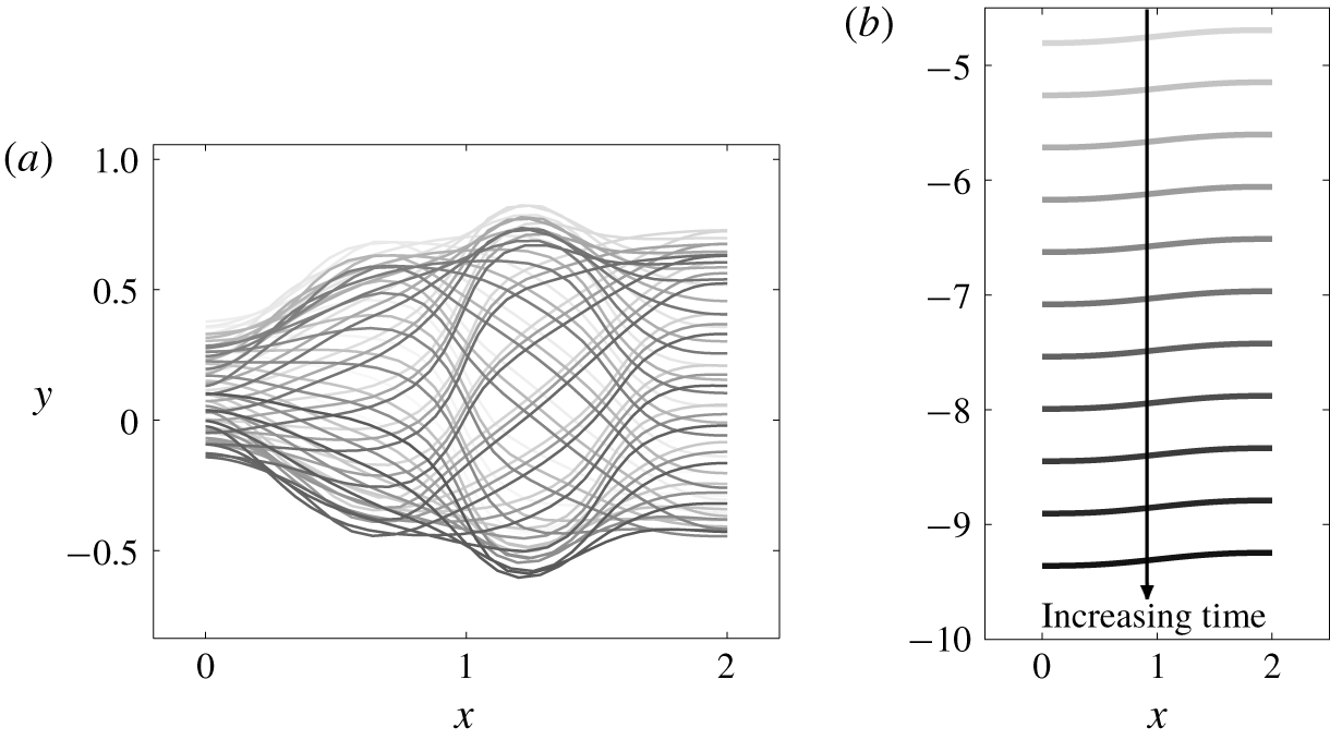
 $y$ direction. The motion is shown enlarged in figure 24(a). The corresponding vortex wake, shown in figure 23 (middle column, bottom row) is more complex than a von Kármán vortex street. At the upper right of figure 23 are approximately straight-line wakes, corresponding to membranes that translate steadily with a constant shape, e.g. the enlarged example in figure 24(b). Here the vortex wakes have zero strength density in the large-time limit, and so they translate steadily downstream without any self-induced undulatory motion or roll-up.
(Free–free) Membrane snapshots at the large-amplitude regime for (a)  $R_{1}=10^{0}$ and
 $R_{3}=10^{0.5}$ and (b)
 $R_{1}=10^{0.5}$ and
 $R_{3}=10^{2.5}$. The shading of the membrane indicates the different phases in the motion, varying from gray at earlier times to black at current times.

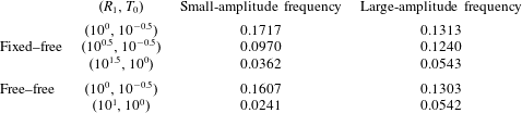
Comparison of frequencies in the small-amplitude and large-amplitude regimes with  $R_{3}=10^{1.5}$ for three pairs of
 $(R_{1},T_{0})$ at the flutter and divergence region for fixed–free and free–free membranes.

Our final results are a brief comparison of membrane frequencies in the small-amplitude exponential growth regime, the focus of previous membrane flutter studies, and the large-amplitude steady-state regime. The top three rows of table 2 compare the small- and large-amplitude frequencies of three fixed–free membranes, shown in figure 9 (at  $R_{3}=10^{1.5}$), that become unstable through flutter and divergence and oscillate with a single dominant frequency. The bottom two rows compare the frequencies for two free–free membranes that also oscillate with single dominant frequencies. We note that the frequency may become significantly lower or higher as the membranes transition from small to large amplitude. It is unclear in general if aspects of the large amplitude motion can be inferred from the shapes and frequencies of the unstable modes in the linearized, small-amplitude regime.
4 Conclusions
In this work we have studied the flutter instability and large amplitude dynamics of thin membranes. These are made of elastic materials – e.g. rubber, textile fabric or the skin of swimming or flying animals – with Young’s moduli sufficiently small that stretching provides the primary resistance to fluid forces and bending resistance is negligible. Previous studies have considered the flutter instability of membranes with fixed ends. We find that all such membranes become unstable by divergence below a critical pretension  $T_{0}$ close to the value identified in previous studies. Surprisingly, we find that all cases that exhibit large (but physically reasonable) deflections converge to states of steady deflection with single humps that are almost fore-aft symmetric, and the deflections scale as
 $1/\sqrt{R_{3}}$, where
 $R_{3}$ is the stretching modulus. These deformations are similar to those found with linearized models that assumed steady deflection at a fixed angle of attack (Waldman & Breuer Reference Waldman and Breuer2017; Tzezana & Breuer Reference Tzezana and Breuer2019).
We then considered membranes with the leading edge fixed and the trailing edge free, and found a wide range of unsteady dynamics, somewhat similar to those seen in studies of flapping plates or flags. The critical pretension  $T_{0}$ now depends on the membrane mass density
 $R_{1}$. Membranes become unstable with divergence or with a combination of flutter and divergence in some cases near the stability boundary. The large-amplitude dynamics are independent of the pretension except close to the stability boundary, where the dynamics are in some cases more periodic and have smaller amplitudes. The dynamics depend most strongly on the membrane mass density
 $R_{1}$. At the largest
 $R_{1}$ studied we find the smallest oscillation frequencies and largest membrane deflections corresponding to somewhat chaotic and asymmetrical membrane motions. Here the mean temporal frequency scales as
 $1/\sqrt{R_{1}}$. As
 $R_{1}$ decreases, the membrane motions become more periodic and symmetrical, and with larger spatial frequency components (sharper curvatures and more zero crossings). At
 $R_{1}\leqslant 0.1$ the motions become more chaotic again, with much finer spatial features that are difficult to resolve numerically.
With both edges free, the membrane motions show two new features – a vertical translational component that may be nearly steady or oscillatory, and a non-zero slope. The combination of the two yields a small angle of attack with respect to the oncoming flow. The translational motion may be steady, periodic or chaotic, and switch among these states with small changes of parameters. Superposed on the translational motions with non-zero slope are modes with oscillatory spatial and temporal features, similar to those in the fixed–free case in how they vary with  $T_{0}$,
 $R_{1}$ and
 $R_{3}$.
Membrane (as opposed to beam/plate) flutter with free ends has barely been explored. However, our study shows that these boundary conditions allow for a much wider range of membrane dynamics with potential future applications in enhancing the performance of membrane wings (Tamai et al. Reference Tamai, Murphy and Hu2008; Arbós-Torrent et al. Reference Arbós-Torrent, Ganapathisubramani and Palacios2013), sails (Colgate Reference Colgate1996; Kimball Reference Kimball2009), and energy harvesting by membranes mounted on tensegrity structures (Sunny et al. Reference Sunny, Sultan and Kapania2014; Yang & Sultan Reference Yang and Sultan2016). Extensional deformations may be used in conjunction with (Drachinsky & Raveh Reference Drachinsky and Raveh2016; Chatterjee & Bryant Reference Chatterjee and Bryant2018) or as an alternative to bending-dominated deformations for energy harvesting, e.g. the flutter of piezoelectric beams and bilayers (Erturk et al. Reference Erturk, Vieira, De Marqui and Inman2010; Doaré & Michelin Reference Doaré and Michelin2011; Giacomello & Porfiri Reference Giacomello and Porfiri2011; Kim et al. Reference Kim, Cossé, Cerdeira and Gharib2013; Porfiri & Peterson Reference Porfiri and Peterson2013; Wang et al. Reference Wang, Alben, Li and Young2016; Orrego et al. Reference Orrego, Shoele, Ruas, Doran, Caggiano, Mittal and Kang2017).
Acknowledgements
We acknowledge support from a Rackham International Student Fellowship (University of Michigan) to C.M.
Declaration of interests
The authors report no conflict of interest.
Supplementary movies and materials
Supplementary movies and materials are available at https://doi.org/10.1017/jfm.2020.153.
Appendix A. Pressure jump equation
In this appendix we derive the equation for the pressure jump  $[p](\unicode[STIX]{x1D6FC},t)$ across the membrane, given by (2.19), as in Alben (Reference Alben2012) but for an extensible body. We use vector notation instead of complex notation.
The Euler momentum equation given by
 $$\begin{eqnarray}\unicode[STIX]{x2202}_{t}\boldsymbol{u}(\boldsymbol{x},t)+\boldsymbol{u}(\boldsymbol{x},t)\boldsymbol{\cdot }\unicode[STIX]{x1D735}\boldsymbol{u}(\boldsymbol{x},t)=-\unicode[STIX]{x1D735}p(\boldsymbol{x},t),\end{eqnarray}$$
determines the velocity of the fluid flow  $\boldsymbol{u}(\boldsymbol{x},t)$ at a point
 $\boldsymbol{x}$ in the fluid. We want to calculate the fluid pressure at a point in the fluid that is adjacent to and follows a material point
 $\boldsymbol{X}(\unicode[STIX]{x1D6FC},t)$ on the membrane. The rate of change of fluid velocity at such a point is
 $$\begin{eqnarray}\frac{\text{d}}{\text{d}t}\boldsymbol{u}(\boldsymbol{X}(\unicode[STIX]{x1D6FC},t),t)=\unicode[STIX]{x2202}_{t}\boldsymbol{u}(\boldsymbol{x},t)|_{\boldsymbol{x}=\boldsymbol{X}(\unicode[STIX]{x1D6FC},t)}+(\unicode[STIX]{x2202}_{t}\boldsymbol{X}(\unicode[STIX]{x1D6FC},t)\boldsymbol{\cdot }\unicode[STIX]{x1D735})\boldsymbol{u}(\boldsymbol{x},t)|_{\boldsymbol{x}=\boldsymbol{X}(\unicode[STIX]{x1D6FC},t)}.\end{eqnarray}$$
We replace the first term in (A 1) using the same term in (A 2) (the first term on the right-hand side). This yields the pressure gradient at a point that moves with  $\boldsymbol{X}(\unicode[STIX]{x1D6FC},t)$. Since the fluid velocity is discontinuous across the membrane, we actually need to do this separately for points that tend toward
 $\boldsymbol{X}(\unicode[STIX]{x1D6FC},t)$ from each side of the membrane. We obtain
 $$\begin{eqnarray}\frac{\text{d}}{\text{d}t}\boldsymbol{u}(\boldsymbol{X}(\unicode[STIX]{x1D6FC},t),t)^{\pm }+((\boldsymbol{u}(\boldsymbol{x},t)-\unicode[STIX]{x2202}_{t}\boldsymbol{X})\boldsymbol{\cdot }\unicode[STIX]{x1D735}\boldsymbol{u}(\boldsymbol{x},t)|_{\boldsymbol{x}=\boldsymbol{X}(\unicode[STIX]{x1D6FC},t)})^{\pm }=-(\unicode[STIX]{x1D735}p(\boldsymbol{x},t)|_{\boldsymbol{ x}=\boldsymbol{X}(\unicode[STIX]{x1D6FC},t)})^{\pm },\end{eqnarray}$$
using ‘ $+$’ for the side toward which the membrane normal
 $\hat{\boldsymbol{n}}$ is directed and ‘
 $-$’ for the other side.
Next, we decompose the fluid velocity into components tangential and normal to the membrane. The normal component matches that of the membrane,  $\unicode[STIX]{x1D708}$ in (2.21b). The tangential component of the fluid velocity may be written in terms of its jump across the membrane, the same as the vortex sheet strength
 $\unicode[STIX]{x1D6FE}$ (Saffman Reference Saffman1992),
 $$\begin{eqnarray}(\boldsymbol{u}^{+}-\boldsymbol{u}^{-})\boldsymbol{\cdot }\hat{\boldsymbol{s}}=-\unicode[STIX]{x1D6FE},\end{eqnarray}$$
and the average of the tangential components of the fluid velocity on the two sides of the membrane, denoted  $\unicode[STIX]{x1D707}$. Combining the tangential and normal components, we have
 $$\begin{eqnarray}\boldsymbol{u}^{\pm }=\left(\unicode[STIX]{x1D707}\mp \frac{\unicode[STIX]{x1D6FE}}{2}\right)\hat{\boldsymbol{s}}+\unicode[STIX]{x1D708}\hat{\boldsymbol{n}}.\end{eqnarray}$$
We take the difference of (A 3) on the ‘ $+$’ and ‘
 $-$’ sides:
 $$\begin{eqnarray}\displaystyle & & \displaystyle \frac{\text{d}}{\text{d}t}(\boldsymbol{u}^{+}(\boldsymbol{X}(\unicode[STIX]{x1D6FC},t),t)-\boldsymbol{u}^{-}(\boldsymbol{X}(\unicode[STIX]{x1D6FC},t),t))+((\boldsymbol{u}^{+}(\boldsymbol{x},t)-\unicode[STIX]{x2202}_{t}\boldsymbol{X})\boldsymbol{\cdot }\unicode[STIX]{x1D735}\boldsymbol{u}^{+}(\boldsymbol{x},t)|_{\boldsymbol{x}=\boldsymbol{X}(\unicode[STIX]{x1D6FC},t)})\nonumber\\ \displaystyle & & \displaystyle \quad -\,((\boldsymbol{u}^{-}(\boldsymbol{x},t)-\unicode[STIX]{x2202}_{t}\boldsymbol{X})\boldsymbol{\cdot }\unicode[STIX]{x1D735}\boldsymbol{u}^{-}(\boldsymbol{x},t)|_{\boldsymbol{x}=\boldsymbol{X}(\unicode[STIX]{x1D6FC},t)})=-(\unicode[STIX]{x1D735}p(\boldsymbol{x},t)^{+}-\unicode[STIX]{x1D735}p(\boldsymbol{x},t)^{-})|_{\boldsymbol{x}=\boldsymbol{X}(\unicode[STIX]{x1D6FC},t)}.\nonumber\\ \displaystyle & & \displaystyle\end{eqnarray}$$
We then take the tangential component of (A 6), term by term. Using (A 5),
 $$\begin{eqnarray}\hat{\boldsymbol{s}}\boldsymbol{\cdot }\frac{\text{d}}{\text{d}t}(\boldsymbol{u}^{+}(\boldsymbol{X}(\unicode[STIX]{x1D6FC},t),t)-\boldsymbol{u}^{-}(\boldsymbol{X}(\unicode[STIX]{x1D6FC},t),t))=\hat{\boldsymbol{s}}\boldsymbol{\cdot }\unicode[STIX]{x2202}_{t}(-\unicode[STIX]{x1D6FE}(\unicode[STIX]{x1D6FC},t)\hat{\boldsymbol{s}}(\unicode[STIX]{x1D6FC},t))=-\unicode[STIX]{x2202}_{t}\unicode[STIX]{x1D6FE}(\unicode[STIX]{x1D6FC},t).\end{eqnarray}$$
Using
 $$\begin{eqnarray}\unicode[STIX]{x2202}_{t}\boldsymbol{X}=\unicode[STIX]{x1D70F}\hat{\boldsymbol{s}}+\unicode[STIX]{x1D708}\hat{\boldsymbol{n}},\end{eqnarray}$$
and (A 5),
 $$\begin{eqnarray}\hat{\boldsymbol{s}}\boldsymbol{\cdot }[(\boldsymbol{u}^{\pm }(\boldsymbol{x},t)-\unicode[STIX]{x2202}_{t}\boldsymbol{X})\boldsymbol{\cdot }\unicode[STIX]{x1D735}\boldsymbol{u}^{\pm }(\boldsymbol{x},t)]|_{\boldsymbol{ x}=\boldsymbol{X}(\unicode[STIX]{x1D6FC},t)}=\left(\unicode[STIX]{x1D707}\mp \frac{\unicode[STIX]{x1D6FE}}{2}-\unicode[STIX]{x1D70F}\right)\left[\unicode[STIX]{x2202}_{s}\left(\unicode[STIX]{x1D707}\mp \frac{\unicode[STIX]{x1D6FE}}{2}\right)-\unicode[STIX]{x1D708}\unicode[STIX]{x1D705}\right].\end{eqnarray}$$
The difference of the ‘ $+$’ and ‘
 $-$’ terms on the right-hand side of (A 9) is
 $$\begin{eqnarray}-(\unicode[STIX]{x1D707}-\unicode[STIX]{x1D70F})\unicode[STIX]{x2202}_{s}\unicode[STIX]{x1D6FE}-\unicode[STIX]{x1D6FE}(\unicode[STIX]{x2202}_{s}\unicode[STIX]{x1D707}-\unicode[STIX]{x1D708}\unicode[STIX]{x1D705}).\end{eqnarray}$$
The tangential component of the right-hand side of (A 6) is
 $$\begin{eqnarray}-\unicode[STIX]{x2202}_{s}[p]_{-}^{+}(\boldsymbol{x},t)|_{\boldsymbol{ x}=\boldsymbol{X}(\unicode[STIX]{x1D6FC},t)}.\end{eqnarray}$$
Combining (A 7), (A 10) and (A 11), the tangential component of (A 6) is
 $$\begin{eqnarray}\unicode[STIX]{x2202}_{t}\unicode[STIX]{x1D6FE}+(\unicode[STIX]{x1D707}-\unicode[STIX]{x1D70F})\unicode[STIX]{x2202}_{s}\unicode[STIX]{x1D6FE}+\unicode[STIX]{x1D6FE}(\unicode[STIX]{x2202}_{s}\unicode[STIX]{x1D707}-\unicode[STIX]{x1D708}\unicode[STIX]{x1D705})=\unicode[STIX]{x2202}_{s}[p]_{-}^{+},\end{eqnarray}$$
or using  $\unicode[STIX]{x1D6FC}$-derivatives,
 $$\begin{eqnarray}\unicode[STIX]{x2202}_{\unicode[STIX]{x1D6FC}}s\unicode[STIX]{x2202}_{t}\unicode[STIX]{x1D6FE}+(\unicode[STIX]{x1D707}-\unicode[STIX]{x1D70F})\unicode[STIX]{x2202}_{\unicode[STIX]{x1D6FC}}\unicode[STIX]{x1D6FE}+\unicode[STIX]{x1D6FE}(\unicode[STIX]{x2202}_{\unicode[STIX]{x1D6FC}}\unicode[STIX]{x1D707}-\unicode[STIX]{x2202}_{\unicode[STIX]{x1D6FC}}s\unicode[STIX]{x1D708}\unicode[STIX]{x1D705})=\unicode[STIX]{x2202}_{\unicode[STIX]{x1D6FC}}[p]_{-}^{+}.\end{eqnarray}$$
Appendix B. Numerical approximations
Vortex sheet computations can become expensive for long-time simulations. For a membrane in an oncoming flow (unidirectional and steady far upstream), the vortex wake is advected away from the membrane and it is possible to decrease resolution of the far-field wake (similarly to Alben (Reference Alben2009)) with only a small effect on the membrane and near-membrane wake dynamics.
(Free–free) Surface plot of the mean frequency computed from the time series of the circulation, once the membranes have entered the large-amplitude regime with  $T_{0}=10^{-2}$. The corresponding power spectra for each of the membranes are also shown on the surface plot. The data in the right-bottom corner are obtained for a shorter time and so we neglect the computational results for those values of
 $R_{1}$ and
 $R_{3}$.

We briefly describe the numerical approximations used to compute the wake dynamics in this work. For computational efficiency, we use a higher resolution near the membrane’s trailing edge, and we prune the vortex wake in the far field. Once the free vortex sheet gets longer than one thousand points, we retain only the points of the free vortex sheet at local extrema of the circulation, to approximately maintain the zeroth and first moments of vorticity but using a small number of points. Because this portion of the sheet is far from the membrane, this approximation has a negligible effect on the dynamics. Examples are shown in figures 17 and 23, where the prescribed membrane parameters are  $(R_{1},R_{3})=(10^{0.5},10^{1})$ and
 $(R_{1},R_{3})=(10^{0},10^{0.5})$, respectively.
We also use a point insertion/deletion scheme, but only sufficiently far from the membrane’s trailing edge (e.g. implemented only more than 80 wake points from the trailing edge). As the free wake evolves, the distance between two consecutive points can increase beyond a given parameter  $d_{1}$ (a fixed fraction of the wake smoothing parameter
 $\unicode[STIX]{x1D6FF}$), and if this occurs, we insert new points using cubic interpolation to maintain wake resolution (Krasny Reference Krasny1987; Nitsche & Krasny Reference Nitsche and Krasny1994; Alben Reference Alben2009). Similarly, at each time step, we check the distance between three consecutive points and if the distance between the first and third point is less than a specified threshold value
 $d_{2}$, then we delete the point in between the two to reduce the computational cost. During both processes, we always ensure that the total circulation is conserved for all times to satisfy Kelvin’s circulation theorem.
Appendix C. Membrane frequencies in the free–free case
Since we have determined where in the parameter space the membrane is unstable, we can characterize the large-amplitude dynamics using the mean frequency and study how it depends on  $R_{1}$ and
 $R_{3}$. We focus on the region where reliable frequency data can be obtained. As we have done previously, we compute the power spectrum from a plot of the circulation versus time, when the membrane has reached large-amplitude dynamics. In figure 25 we see that, in general, the frequency decreases with increasing
 $R_{1}$. For
 $R_{1}=10^{0.5}$ and
 $R_{3}$ ranging from
 $10^{2}$ to
 $10^{4}$, the membranes translate steadily (see figure 19) and the wake circulation tends to zero at large times. Therefore, the power spectra for those cases are zero and we omit them.