1 Introduction
Heat or mass transport in disperse multiphase systems is of much relevance in both natural and industrial settings. We consider a system where the disperse and continuous phases are both Newtonian liquids, and the disperse phase (drop) volume fraction is small enough for interactions to be neglected. The problem then reduces to transport to or from a single drop in a Newtonian ambient undergoing a shearing flow. An ambient linear flow is relevant to neutrally buoyant drops whose size (
 $a$
) is small compared to the scales that characterize the flow such that any complicated flow appears as a linear flow at leading order. The small drop size also implies that viscous effects dominate the transport of momentum and the Reynolds number defined as
 $Re=\dot{\unicode[STIX]{x1D6FE}}a^{2}/\unicode[STIX]{x1D708}$
is therefore small. Here,
 $\dot{\unicode[STIX]{x1D6FE}}$
is a scale for the ambient shear rate and
 $\unicode[STIX]{x1D708}$
is the kinematic viscosity of the ambient fluid. On the other hand, we assume convective effects to dominate heat/mass transport. So, the Péclet number, defined as
 $Pe=\dot{\unicode[STIX]{x1D6FE}}a^{2}/D$
, where
 $D$
is the diffusivity of heat or mass in the ambient fluid, is large. Note that this limit is typical for mass transport problems in liquid phases, in which case the Schmidt number (
 $Sc=Pe/Re$
) is almost always large on account of the small mass diffusivities (Leal Reference Leal2007).
In this work, we investigate the effects of small but finite inertia on the heat transport from drops in ambient planar linear flows in the regime where the near-field exterior streamlines are closed in the Stokesian limit (
 $Re=0$
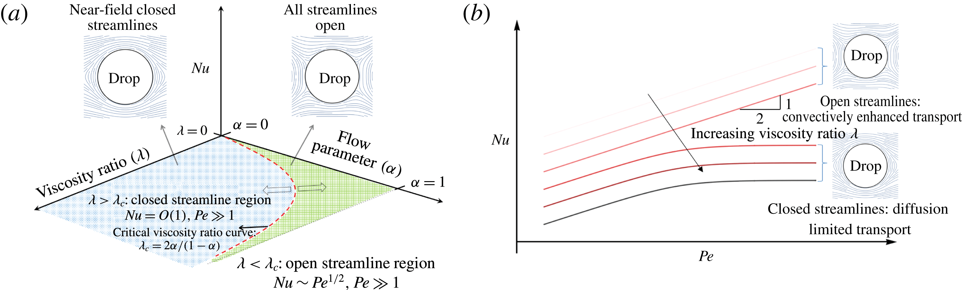
). In a companion paper (Krishnamurthy & Subramanian Reference Krishnamurthy and Subramanian2018), which included a detailed review of earlier related efforts in the literature, it was shown that for drops in the one-parameter family of hyperbolic planar linear flows, the parameter being
 $\unicode[STIX]{x1D6FC}$
, there are two distinct exterior streamline topologies in the Stokesian limit, with profound implications for the transport of heat/mass at large
 $Pe$
(see figure 1). The exterior streamline topology was shown to depend on two parameters (i) the flow-type parameter
 $\unicode[STIX]{x1D6FC}$
above, which measures the relative amounts of extension and vorticity in the ambient (
 $0<\unicode[STIX]{x1D6FC}<1$
for hyperbolic linear flows;
 $\unicode[STIX]{x1D6FC}=0$
for simple shear and
 $\unicode[STIX]{x1D6FC}=1$
for planar extension), and (ii) the drop-to-medium viscosity ratio
 $\unicode[STIX]{x1D706}$
(
 $0<\unicode[STIX]{x1D706}<\infty$
;
 $\unicode[STIX]{x1D706}=0$
corresponds to a bubble, while
 $\unicode[STIX]{x1D706}\rightarrow \infty$
is a rigid particle). For
 $\unicode[STIX]{x1D706}<\unicode[STIX]{x1D706}_{c}$
, all exterior streamlines are open (that is, they originate and terminate at ‘infinity’), while for
 $\unicode[STIX]{x1D706}>\unicode[STIX]{x1D706}_{c}$
a subset of these streamlines in the neighbourhood of the drop is closed. Here,
 $\unicode[STIX]{x1D706}_{c}=2\unicode[STIX]{x1D6FC}/(1-\unicode[STIX]{x1D6FC})$
is the critical viscosity ratio marking the boundary between the two distinct regimes in the (
 $\unicode[STIX]{x1D6FC},\unicode[STIX]{x1D706}$
) plane. In the open streamline regime, the transport is convectively enhanced even in the Stokes limit (
 $Re=0$
), and the Nusselt number (the ratio of total to purely diffusive transport;
 $Nu=1$
for
 $Pe=0$
) has the form
 $Nu={\mathcal{H}}_{o}(\unicode[STIX]{x1D6FC},\unicode[STIX]{x1D706})Pe^{1/2}$
(see figure 1), where
 ${\mathcal{H}}_{o}(\unicode[STIX]{x1D6FC},\unicode[STIX]{x1D706})$
is obtained in terms of a one-dimensional integral via a large
 $Pe$
boundary layer analysis (Krishnamurthy & Subramanian Reference Krishnamurthy and Subramanian2018). However, in the closed streamline regime, the near-field exterior streamlines, on account of being closed, are ineffective in convecting heat away from the drop. The transport at zero
 $Re$
, for long times, is therefore due to slow diffusion across Stokesian isotherms (see Rhines & Young Reference Rhines and Young1983). The Nusselt number, in the limit of large
 $Pe$
, plateaus out to a constant of order unity dependent on the geometry of the closed streamline region (figure 1
b), indicative of a finite convective enhancement. The enhancement factor is approximately 4.5 for simple shear flow (Acrivos Reference Acrivos1971), and is
 $O(1-\unicode[STIX]{x1D6FC})^{-1}$
for
 $\unicode[STIX]{x1D6FC}\rightarrow 1$
(Poe & Acrivos Reference Poe and Acrivos1976).
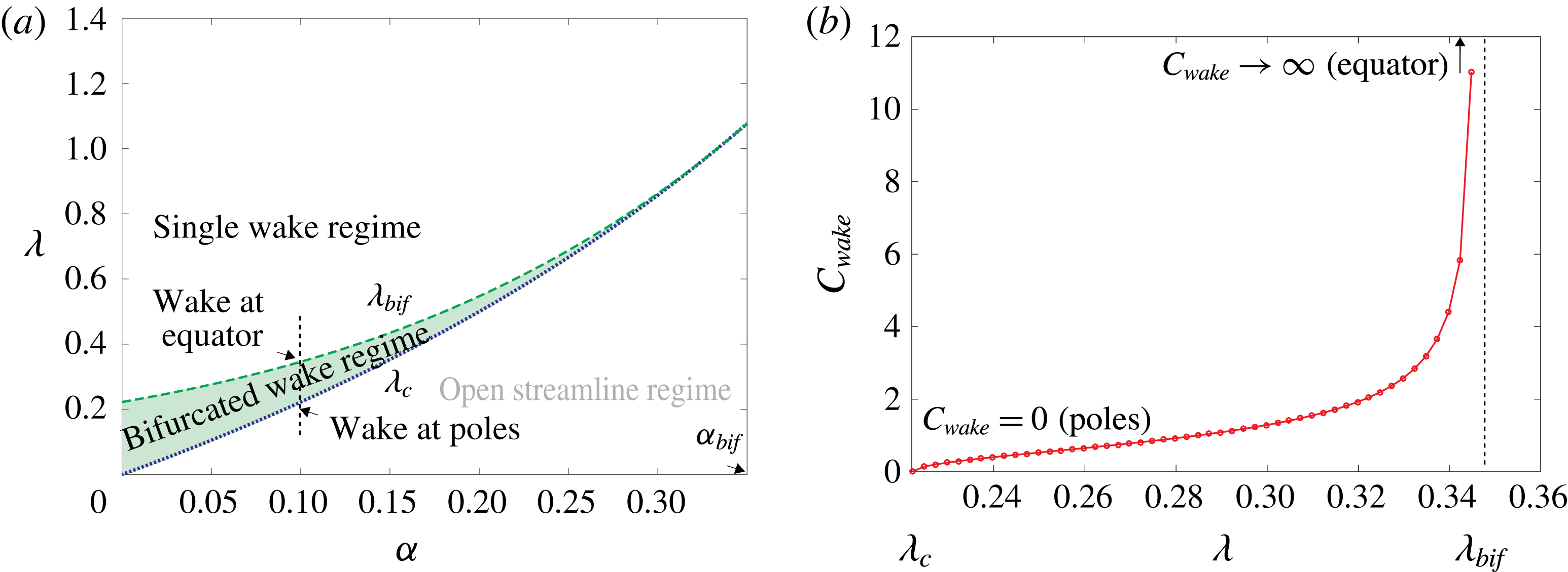
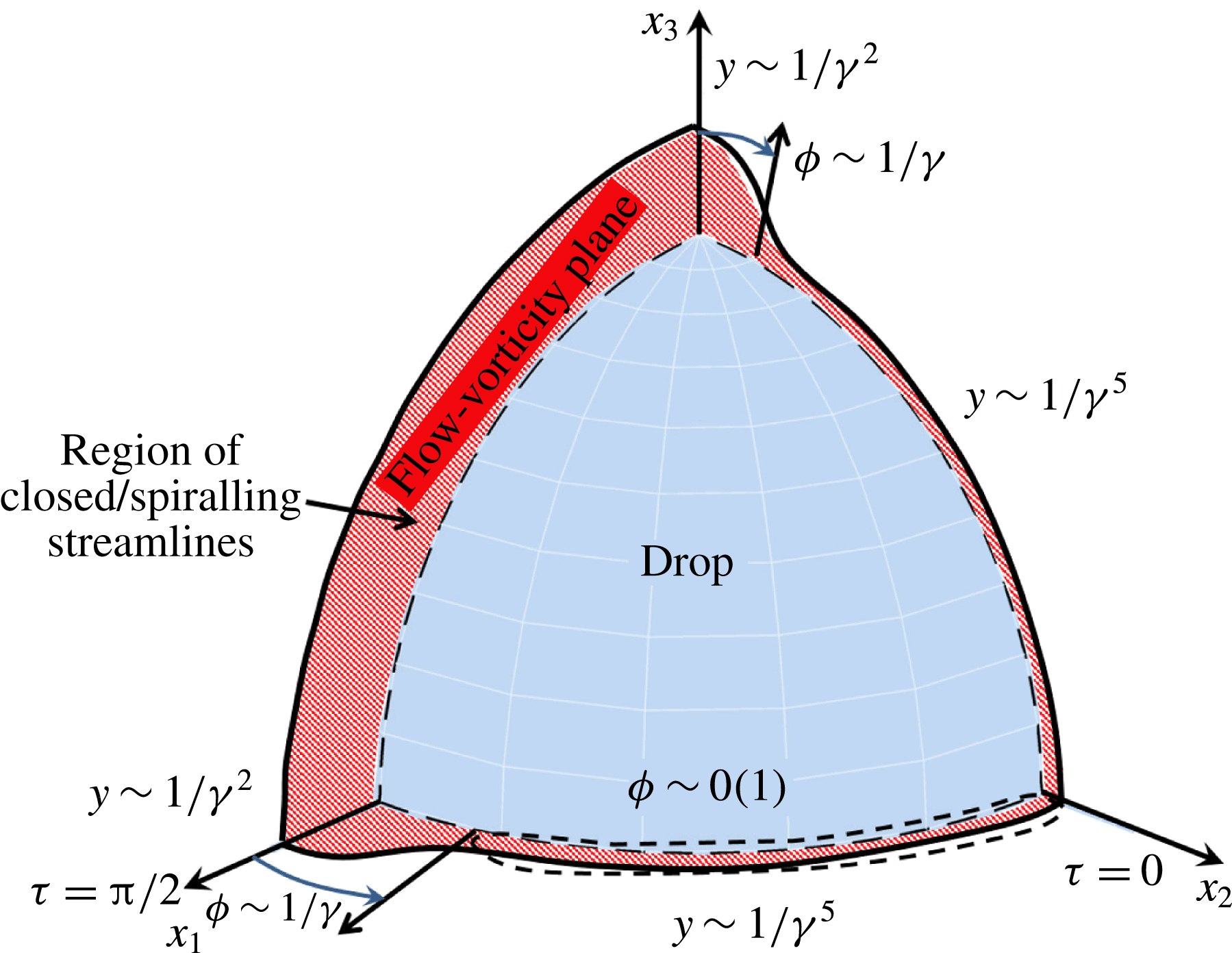
Exterior streamline topology has a profound impact on rate of heat transfer from a drop. (a) Schematic of the (
 $\unicode[STIX]{x1D6FC},\unicode[STIX]{x1D706}$
) plane showing the open and closed streamline regimes and the critical viscosity-ratio curve (
 $\unicode[STIX]{x1D706}_{c}=2\unicode[STIX]{x1D6FC}/(1-\unicode[STIX]{x1D6FC})$
) separating them. (b)
 $Nu\sim Pe^{1/2}$
in the open streamline regime for
 $Re=0$
and
 $Pe\gg 1$
. As
 $\unicode[STIX]{x1D706}$
increases beyond
 $\unicode[STIX]{x1D706}_{c}$
, the near-field Stokesian streamlines are closed, leading to
 $Nu=O(1)$
for
 $Pe\gg 1$
.

While the diffusion-limited scenario above prevails in the Stokesian regime, things are radically different with the addition of a small but finite amount of inertia. Even weak inertial effects transform these closed Stokesian streamlines into tightly spiralling ones at small
 $Re$
, a feature first recognized by Subramanian & Koch (Reference Subramanian and Koch2006a
,Reference Subramanian and Koch
b
). Physically, this is because fluid elements moving around the drop now experience an additional inertial force which leads to a net radial displacement over the period of a complete (Stokesian) orbit. Thus, for any finite
 $Re$
, almost every fluid element comes from, and ultimately goes to, infinity, although the residence time in the vicinity of the drop diverges for
 $Re\rightarrow 0$
. This symmetry breaking role of weak inertia, and the resulting spiralling streamline topology, crucially depends on the dimensionality of the problem. On account of incompressibility, it does not occur when the object is two-dimensional and the flow remains steady; for instance, a cylinder in a simple shear flow at moderate
 $Re$
(Robertson & Acrivos Reference Robertson and Acrivos1970; Kossack & Acrivos Reference Kossack and Acrivos1974); this feature of the two-dimensional problem led some earlier authors to erroneously expect the three-dimensional problem to behave in an analogous manner (Poe & Acrivos Reference Poe and Acrivos1975; Mikulencak & Morris Reference Mikulencak and Morris2004). Since the spiralling inertial streamlines, in three dimensions, are no longer limited to a finite region next to the immersed body, heat can be transported effectively due to convection. The newly formed ‘convective channels’ due to inertia, lead to the Nusselt number again increasing with
 $Pe$
for sufficiently large
 $Pe$
. Thus, for any
 $Re$
however small,
 $Nu$
far exceeds the geometrically determined upper bound attained in the limit
 $Re=0$
,
 $Pe\rightarrow \infty$
. Unlike the open streamline regime, where the effects of inertia are perturbative in nature, in the closed streamline regime, inertia modifies the heat transport at leading order.
The effects of inertia on transport from spherical particles in simple shear flow and planar linear flows, respectively, were considered by Subramanian & Koch (Reference Subramanian and Koch2006a
,Reference Subramanian and Koch
b
), who showed that the circular streamlines near the sphere (rotating due to the ambient vorticity) are transformed into spiralling streamlines due to weak inertia. The maximal centrifugal force, directed radially outward, is experienced by fluid elements in the plane of symmetry, and their outward migration causes other fluid elements to spiral in towards the plane of symmetry. It is this inertial convection that determines the transport for sufficiently large
 $Pe$
. Subramanian & Koch (Reference Subramanian and Koch2006b
) went on to solve the inertial heat transfer problem and obtained an expression for the Nusselt number of the form
 $Nu=0.325(1+\unicode[STIX]{x1D6FC})^{2/3}(RePe)^{1/3}$
in the limit
 $Re\ll 1$
and
 $RePe\gg 1$
. The limit considered implies that convective effects due to inertia dominate diffusion everywhere except in a thin
 $O(RePe)^{-1/3}$
boundary layer on the surface of the particle. The convective enhancement due to inertia, identified by Subramanian & Koch (Reference Subramanian and Koch2006a
,Reference Subramanian and Koch
b
) in the limit
 $Re\ll 1$
, persists even when
 $Re$
is of order unity (Yang et al.
Reference Yang, Zhang, Koch and Yin2011), highlighting the relevance of this result to applications.
The finite slip on the drop surface implies that any convective enhancement due to inertia will lead to a transport rate that is asymptotically larger than that for a rigid particle for large
 $Pe$
. Simple scaling arguments lead to
 $Nu\propto (RePe)^{1/2}$
for a drop, while
 $Nu\propto (RePe)^{1/3}$
for a rigid particle, as seen above, in the limit
 $Re\ll 1,RePe\gg 1$
. The transport problem for drops, however, poses several additional challenges. While for the case of solid particles, there is an annular region of closed streamlines for any finite amount of vorticity in the ambient linear flow (Subramanian & Koch Reference Subramanian and Koch2006b
), for drops, as already mentioned above, the near-field exterior streamlines are closed only when
 $\unicode[STIX]{x1D706}>\unicode[STIX]{x1D706}_{c}=2\unicode[STIX]{x1D6FC}/(1-\unicode[STIX]{x1D6FC})$
; one therefore expects a complicated parametric dependence for
 $Nu$
when transitioning between the open and closed streamline regimes. Secondly, even within the closed streamline regime, the surface and near-field streamlines for a drop are more complicated than the approximately circular near-field streamlines of a solid particle (Subramanian & Koch Reference Subramanian and Koch2006b
). It was shown in Krishnamurthy & Subramanian (Reference Krishnamurthy and Subramanian2018) that the surface streamlines for a drop in both the open and closed streamline regimes are generalized Jeffery orbits with an
 $(\unicode[STIX]{x1D6FC},\unicode[STIX]{x1D706})$
-dependent aspect ratio (Jeffery orbits denote the aspect-ratio-dependent inertialess trajectories of a rigid axisymmetric particle in a simple shear flow; see Jeffery Reference Jeffery1922). This effective aspect ratio is the geometric aspect ratio of a spheroid in a simple shear flow that would have the same orientational trajectories as the surface streamlines in the linear flow with specified
 $\unicode[STIX]{x1D6FC}$
(Leal & Hinch Reference Leal and Hinch1971). While the surface streamlines in the open streamline regimes have imaginary aspect ratios, and are actually finite open curves beginning and ending at stagnation points on the drop surface, those for
 $\unicode[STIX]{x1D706}>\unicode[STIX]{x1D706}_{c}$
are true orbits with a real-valued aspect ratio. The identification with Jeffery orbits implies that the surface streamlines for any
 $\unicode[STIX]{x1D706}>\unicode[STIX]{x1D706}_{c}$
are (non-planar) spherical ellipses rather than circles; for
 $\unicode[STIX]{x1D706}\rightarrow \unicode[STIX]{x1D706}_{c}^{+}$
, corresponding to a diverging effective aspect ratio, the orbits have a nearly meridional character as is known from viscous slender-body theory (Subramanian & Koch Reference Subramanian and Koch2005). The non-axisymmetric surface streamline geometry makes an analytical solution of the convective transport problem more challenging. A third (unanticipated) challenge is the non-trivial reversal of the inertial force acting on the fluid elements as they spiral around the drop, in certain regions of the (
 $\unicode[STIX]{x1D6FC},\unicode[STIX]{x1D706}$
) plane. This is in contrast to the rigid particle case where the inertial force, at
 $O(Re)$
, is always directed towards the plane of symmetry of the ambient flow. This leads to a qualitatively different topology of the wake for a drop for certain combinations of
 $\unicode[STIX]{x1D6FC}$
and
 $\unicode[STIX]{x1D706}$
.
Based on the above identification of surface streamlines with Jeffery orbits, we present a novel solution methodology for the heat/mass transport problem at large
 $Pe$
, using a transformation of the governing convection diffusion to a non-orthogonal surface-streamline-aligned coordinate system. A version of this coordinate system was used earlier, in Krishnamurthy & Subramanian (Reference Krishnamurthy and Subramanian2018), for analysing the large-
 $Pe$
transport in the open streamline regime although, as mentioned above, the open surface streamlines in this regime are not true orbits, and correspond to imaginary aspect ratios. The inertial transport problem analysed here requires a non-trivial generalization of the aforementioned Jeffery-orbit-based coordinate system, defined on the drop surface, to three dimensions. The analogue of the radial coordinate used in the open streamline analysis is now defined using the near-field invariant streamsurfaces of the exterior Stokes flow; the analogues of these surfaces, for a solid particle, were originally identified by Cox, Zia & Mason (Reference Cox, Zia and Mason1968), and those for a drop were examined in Krishnamurthy & Subramanian (Reference Krishnamurthy and Subramanian2018). The generalization mentioned above is required because it is these streamsurfaces, and not spheres concentric with the drop, that are nearly isothermal for large
 $Pe$
. Transforming to a coordinate system based on the topology of the Stokes streamsurfaces therefore allows a significant simplification of the fully three-dimensional boundary layer analysis; in particular, it allows for a parallel to be drawn with the (much) simpler axisymmetric problem that arises for the analogous inertial transport problem involving a solid particle (Subramanian & Koch Reference Subramanian and Koch2006a
,Reference Subramanian and Koch
b
). Importantly, the methodology allows one to finally derive a closed-form expression for the Nusselt number characterizing convective transport from a drop in the presence of small but finite inertia.
1.1 A guide to the paper
We now give a rather detailed guide to the rest of the paper, referencing the salient points of the analysis including key equations and results. The methodology presented here leads to a considerable simplification of the original transport problem, a drop in a shearing flow with a closed streamline topology, and should also be more generally applicable. However, the details are complicated, and lead to a rather lengthy analysis. Thus, the intent of this section to sketch out a map for the main results that appear in the following sections, so a general reader is able to grasp the principal points of the analysis without being bogged down by specific calculational details.
After writing down the governing equations in § 2.1, we briefly describe the streamline topology for the Stokesian case (
 $Re=0$
) in § 2.2. Importantly, we examine the closed streamline region that exists at
 $Re=0$
, and show that the surface streamlines may be regarded as Jeffery orbits with a flow and viscosity-ratio-dependent aspect ratio. This insight allows one to define a non-orthogonal
 $(C,\unicode[STIX]{x1D70F})$
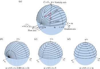
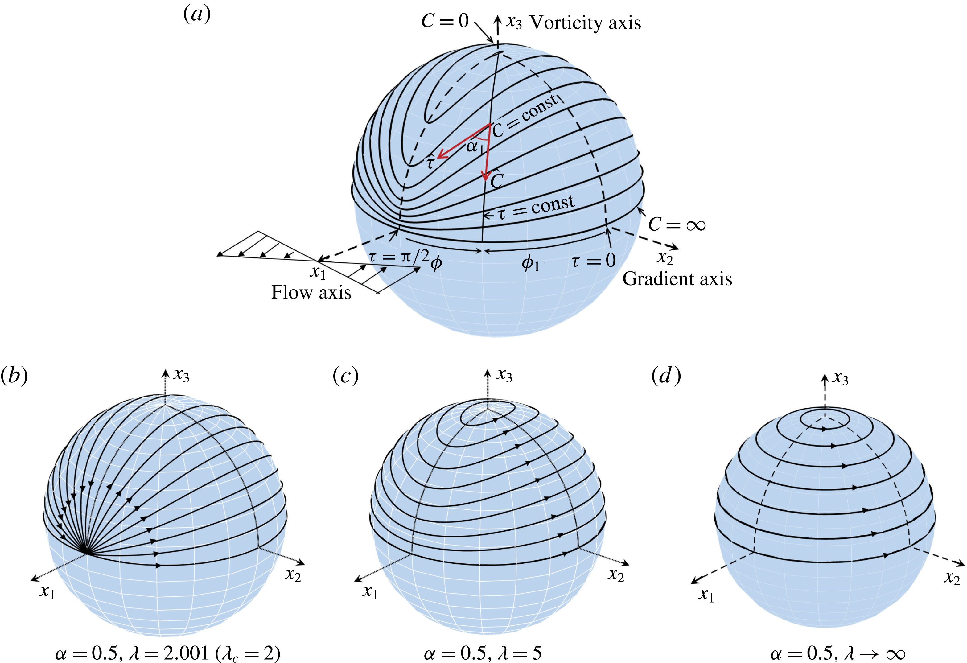
coordinate system on the drop surface (see (2.7)–(2.8)). Here, each closed streamline is defined by an orbit constant
 $C$
and the phase along the orbit
 $\unicode[STIX]{x1D70F}$
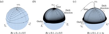
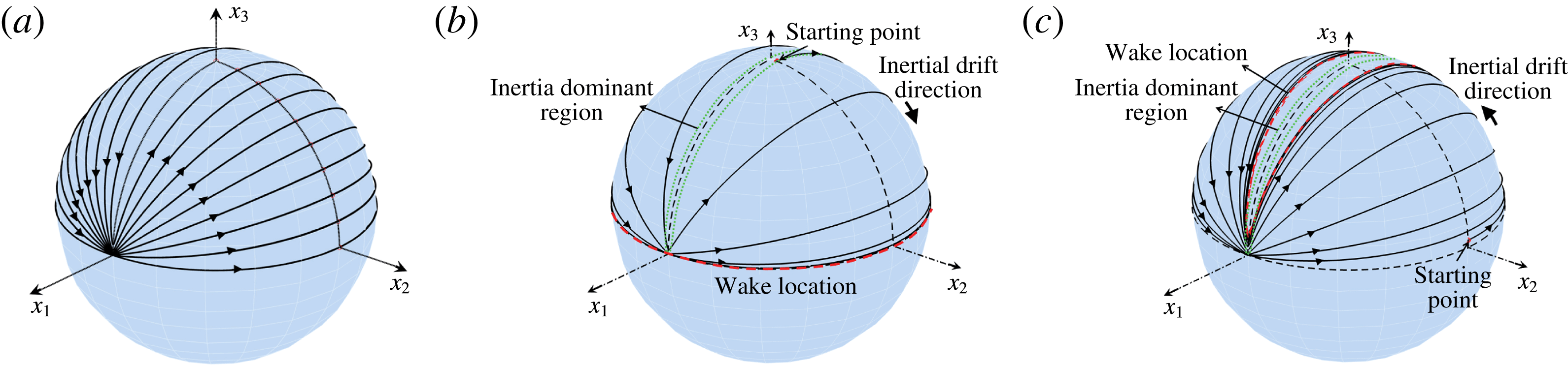
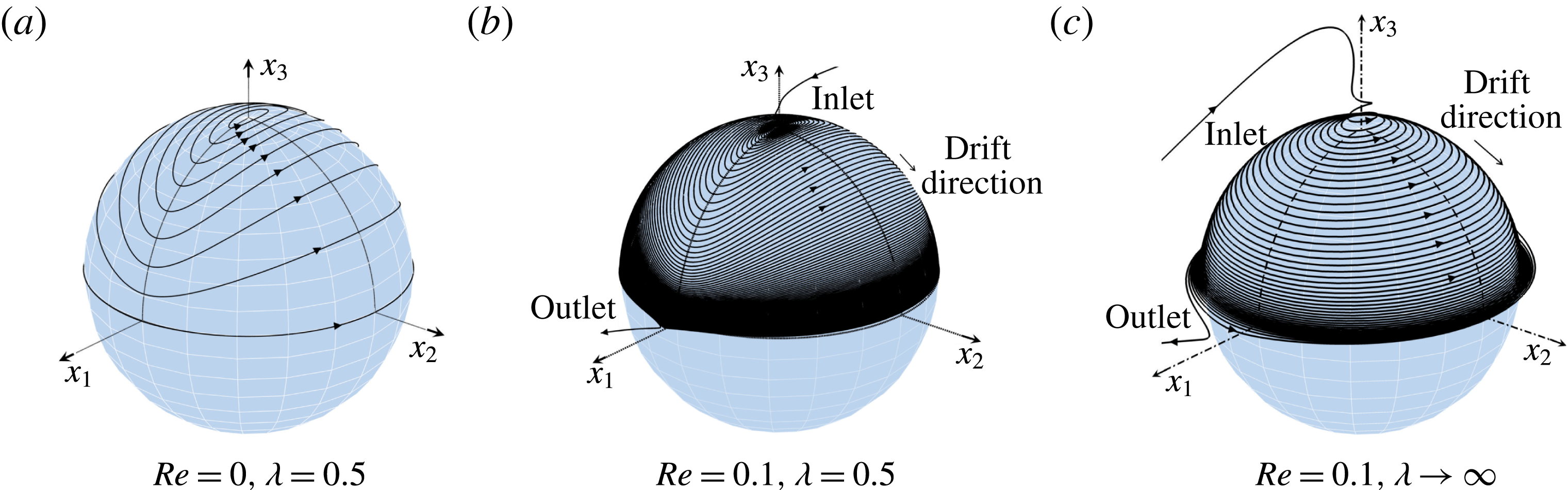
(figure 2). Next, we show in § 2.3 that, with the addition of inertia, the streamlines are no longer closed orbits and are transformed to spiralling streamlines that drift along the drop surface (figure 3). In § 2.3, we argue that the large-
 $Pe$
analysis of the inertial transport requires one to generalize the
 $(C,\unicode[STIX]{x1D70F})$
coordinate system to three dimensions using the near-field Stokes streamsurfaces outside the drop as the new radial coordinate
 $y_{m}$
(see (2.33)). For
 $Re=0$
, the streamlines are defined by an orbit constant
 $C$
, a given value of
 $y_{m}$
, and with
 $\unicode[STIX]{x1D70F}$
(the phase) varying along the orbit. With the addition of inertia, the streamlines are no longer closed and inertia leads to a net drift along the
 $C$
and
 $y_{m}$
directions, this drift being responsible for the convectively enhanced transport.
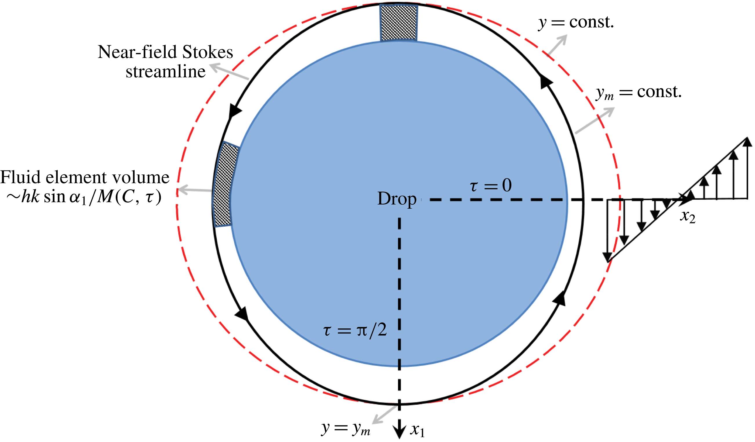
(a) Schematic of the coordinate system used, showing the flow, gradient and vorticity axes for an ambient simple shear flow; the same axis labels are used for other planar hyperbolic linear flows. The surface streamlines on the drop correspond to the closed streamline regime (
 $\unicode[STIX]{x1D706}>\unicode[STIX]{x1D706}_{c}$
). The contravariant unit vectors of the
 $(C,\unicode[STIX]{x1D70F})$
coordinate system are depicted along with the constant-
 $C$
and constant-
 $\unicode[STIX]{x1D70F}$
curves (
 $0\leqslant C<\infty$
and
 $0\leqslant \unicode[STIX]{x1D70F}\leqslant 2\unicode[STIX]{x03C0}$
). (b–d) Increasing
 $\unicode[STIX]{x1D706}$
at a fixed
 $\unicode[STIX]{x1D6FC}$
(
 $=0.5$
) changes the geometry of the closed streamlines which, for a general
 $\unicode[STIX]{x1D706}$
, are spherical ellipses. For
 $\unicode[STIX]{x1D706}\rightarrow \unicode[STIX]{x1D706}_{c}^{+}$
, the streamlines have a nearly meridional character, while for
 $\unicode[STIX]{x1D706}\rightarrow \infty$
, the limiting case of a solid particle, the surface streamlines reduce to plane circles.
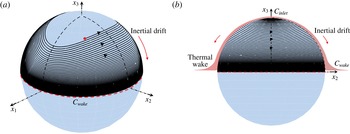
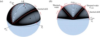
Effects of finite inertia on the Stokesian closed streamline topology. (a) At
 $Re=0$
, the near-field streamlines are closed Jeffery orbits with an effective aspect ratio
 $\unicode[STIX]{x1D6FE}=3.13$
(
 $\unicode[STIX]{x1D6FC}=0.1,\unicode[STIX]{x1D706}=0.5$
). (b) Small but finite inertia fundamentally alters this topology leading to spiralling streamlines. For the particular choice of parameters,
 $\unicode[STIX]{x1D6FC}=0.1$
and
 $\unicode[STIX]{x1D706}=0.5$
, the finite-
 $Re$
streamlines spiral towards the plane of symmetry. (c) For
 $\unicode[STIX]{x1D706}\rightarrow \infty$
(limit of a solid particle) the spiralling nature persists but each turn of the spiral now resembles a circle. Note that for a solid particle, the surface ‘streamlines’ do not spiral and one needs to go away from the surface to see the spiralling character as in (c); for a drop, however, even the surface streamlines have a spiralling character.
In § 2.4 we transform the governing convection–diffusion equation and boundary conditions to the Jeffery-orbit-aligned coordinate system that, in addition, accounts for the near-field closed Stokes streamsurfaces – the
 $(y_{m},C,\unicode[STIX]{x1D70F})$
coordinate system. The transformed equation is given in (2.12), and later, in (2.39), in a form pertinent to transport across an asymptotically thin boundary layer, anticipating the dominance of diffusion in the
 $y_{m}$
direction. The boundary layer regime analysed corresponds to the limit
 $Re\ll 1$
and
 $RePe\gg 1$
. Subsequent to the coordinate transformation we use a phase-averaging approach (based on the separation of time scales between the rapid differential convection due to the leading-order Stokesian flow, and the slower
 $O(Re)$
inertial convection that sets up the eventual temperature variation in the thermal boundary layer) to derive a
 $\unicode[STIX]{x1D70F}$
-averaged convection diffusion equation that governs transport in the limit
 $Re\ll 1$
,
 $RePe\gg 1$
, and wherein, the thermal boundary layer thickness is only a function of the orbit constant
 $C$
at leading order. This orbit-averaged equation appears in (2.50). The above coordinate transformation and subsequent phase-averaging approach are key steps in the analysis.
Next, based on a self-similar ansatz for the boundary layer temperature field, separate ordinary differential equations governing the temperature field (2.55) and the
 $C$
-dependent boundary layer thickness (2.56) are obtained and solved in § 2.5, allowing for an identification of the single and bifurcated wake regimes, the latter regime arising from a reversal in the direction of the
 $\unicode[STIX]{x1D70F}$
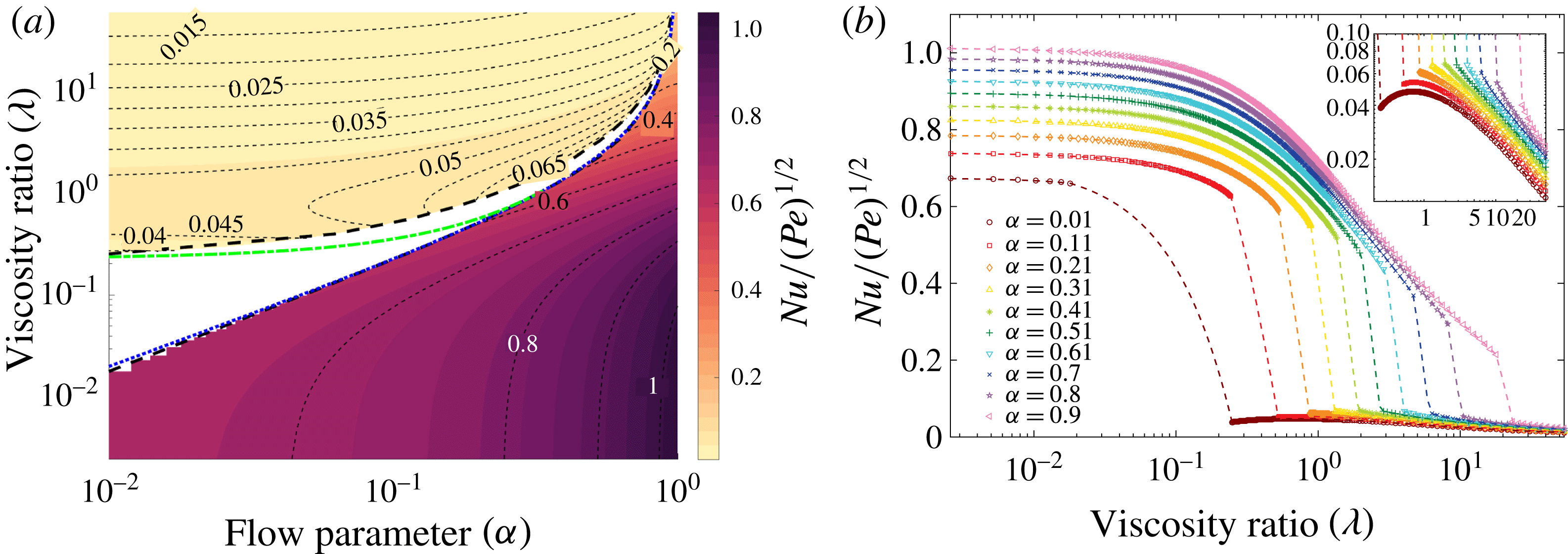
-averaged inertial drift. The final result, just as in the open streamline case (Krishnamurthy & Subramanian Reference Krishnamurthy and Subramanian2018), is an expression for the Nusselt number, equation (2.90), as a function of the flow parameters for the region
 $\unicode[STIX]{x1D706}>\unicode[STIX]{x1D706}_{c}$
in the (
 $\unicode[STIX]{x1D6FC},\unicode[STIX]{x1D706}$
) plane which is given in § 2.6 (figure 9
b).
The final part of the paper contains a discussion of the scaling behaviour of
 $Nu$
in what we term the ‘transition regime’, corresponding to
 $\unicode[STIX]{x1D706}$
close to
 $\unicode[STIX]{x1D706}_{c}$
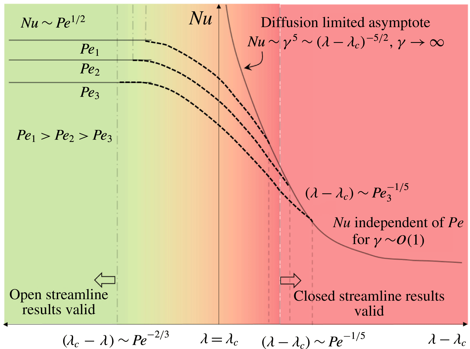
in § 3. Consideration of this regime is important since the leading-order analyses, for
 $Pe\rightarrow \infty$
, in the open and closed streamline regimes yield predictions for the
 $Nu$
-surface that do not connect smoothly across
 $\unicode[STIX]{x1D706}=\unicode[STIX]{x1D706}_{c}$
(see figure 11). The open streamline regime prediction was derived in Krishnamurthy & Subramanian (Reference Krishnamurthy and Subramanian2018), and was shown to remain finite for
 $\unicode[STIX]{x1D706}\rightarrow \unicode[STIX]{x1D706}_{c}^{-}$
; in contrast, the closed streamline regime prediction, given by (2.90), diverges for
 $\unicode[STIX]{x1D706}\rightarrow \unicode[STIX]{x1D706}_{c}^{+}$
. Scaling arguments in § 3 allow one to understand the manner in which the
 $Nu$
-surface, in the (
 $\unicode[STIX]{x1D6FC},\unicode[STIX]{x1D706}$
) plane, transitions smoothly across
 $\unicode[STIX]{x1D706}=\unicode[STIX]{x1D706}_{c}$
for large but finite
 $Pe$
. In particular, we obtain the regions of validity for the open streamline and closed streamline analyses, and thence, the viscosity-ratio interval, given in (3.6), where neither analysis is valid. This allows us to present results for
 $Nu$
in the entire (
 $\unicode[STIX]{x1D6FC},\unicode[STIX]{x1D706}$
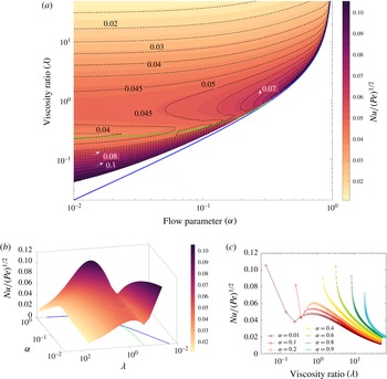
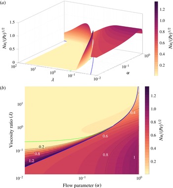
) plane in figures 15 and 16. These may be regarded as the final outcome of the analysis in Krishnamurthy & Subramanian (Reference Krishnamurthy and Subramanian2018) and here (for planar linear flows). In § 4 we present our conclusions, including the directions in which the current analysis may be usefully extended. Herein, we also discuss the various
 $Nu$
-regimes possible for different
 $Sc$
and emphasize the one relevant to applications.
2 Convective transport from drops for small but finite
 $Re$

2.1 Governing equations
The governing equations in dimensionless form for the fluid motion outside the drop, in the presence of inertia, are given by:
 $$\begin{eqnarray}\displaystyle & \displaystyle Re\hspace{2.22198pt}\boldsymbol{u}\boldsymbol{\cdot }\unicode[STIX]{x1D735}\boldsymbol{u}=-\unicode[STIX]{x1D735}p+\unicode[STIX]{x1D6FB}^{2}\boldsymbol{u}, & \displaystyle\end{eqnarray}$$
 $$\begin{eqnarray}\displaystyle & \displaystyle \unicode[STIX]{x1D735}\boldsymbol{\cdot }\boldsymbol{u}=0, & \displaystyle\end{eqnarray}$$
where
 $\boldsymbol{u}$
is the velocity field and
 $p$
is the pressure, with
 $Re\ll 1$
. The inertial velocity field in the drop exterior, which will be used in the subsequent heat transfer analysis, was derived by Raja, Subramanian & Koch (Reference Raja, Subramanian and Koch2010). To
 $O(Re)$
, one may use a regular perturbation analysis, and the exterior velocity field around the spherical drop may be written as:
 $$\begin{eqnarray}\displaystyle \boldsymbol{u}=\boldsymbol{u}^{(0)}(\boldsymbol{r};\unicode[STIX]{x1D6FC},\unicode[STIX]{x1D706})+Re\boldsymbol{u}^{(1)}(\boldsymbol{r};\unicode[STIX]{x1D6FC},\unicode[STIX]{x1D706})+O(Re^{3/2}). & & \displaystyle\end{eqnarray}$$
For a planar linear flow, the Stokes field
 $\boldsymbol{u}^{(0)}$
is well known (Leal Reference Leal2007). The complete expressions for the components of the
 $O(Re)$
velocity field,
 $\boldsymbol{u}^{(1)}$
, are given in Raja et al. (Reference Raja, Subramanian and Koch2010). Although only valid for distances from the drop smaller than the inertial screening length of
 $O(Re^{-1/2})$
, it evidently suffices for purposes of the large-
 $Pe$
boundary layer analysis which only involves the exterior field in the immediate vicinity of the drop. Consideration of the velocity disturbance field on length scales larger than
 $O(Re^{-1/2})$
requires a matched asymptotic expansions approach (Subramanian et al.
Reference Subramanian, Koch, Zhang and Yang2011b
). Here, the limit of small but finite
 $Re$
is examined when in addition,
 $RePe\gg 1$
; this latter limit implies that convection due to the finite-
 $Re$
spiralling flow dominates diffusion everywhere except in a thin thermal boundary layer near the drop surface and in a thermal wake. The wake does not contribute to the transport at leading order, however.
The scalar transport is governed by the convection–diffusion equation, written here in non-dimensional form:
 $$\begin{eqnarray}\displaystyle Pe(\boldsymbol{u}\boldsymbol{\cdot }\unicode[STIX]{x1D735}\unicode[STIX]{x1D6E9})=\unicode[STIX]{x1D6FB}^{2}\unicode[STIX]{x1D6E9}, & & \displaystyle\end{eqnarray}$$
where
 $\unicode[STIX]{x1D6E9}=(T-T_{\infty })/(T_{0}-T_{\infty })$
, where
 $T$
is the temperature field. This is subject to the boundary conditions:
 $$\begin{eqnarray}\displaystyle & \displaystyle \unicode[STIX]{x1D6E9}=1\quad \text{at }r=1\,(\text{Isothermal drop surface with temperature}~T_{0}), & \displaystyle\end{eqnarray}$$
 $$\begin{eqnarray}\displaystyle & \displaystyle \unicode[STIX]{x1D6E9}\rightarrow 0\quad \text{as}~r\rightarrow \infty ~(\text{Ambient temperature is}~T_{\infty }~\text{at infinity}). & \displaystyle\end{eqnarray}$$
Here, we have neglected variations of transport properties, including those of the density and specific heat, with temperature, yielding a forced convection problem. It is worth noting that, in the absence of a body force (such as gravity), this neglect does not immediately alter the streamline topology. In other words, weakly temperature-dependent transport coefficients should preserve the closed streamline topology, although quantitative details such as the critical viscosity ratio demarcating the open and closed streamline regimes will, of course, differ. The condition of isothermality at the drop surface implies neglect of the interior phase resistance, and we have commented in some detail on its validity in Krishnamurthy & Subramanian (Reference Krishnamurthy and Subramanian2018). An important point is the likelihood of inertia-induced Lagrangian chaos for the interior flow. The resulting efficient chaotic mixing within the drop implies that the transport for large
 $Pe$
likely occurs through both interior and exterior boundary layers, and the
 $Nu$
expression derived below (see (2.94) and (2.95)), for the case of a dominant exterior phase resistance, may be readily generalized to the case of comparable phase resistances by multiplication with
 $(k_{i}/k)^{1/2}/[(k_{i}/k)^{1/2}+1]$
for heat transfer (
 $k_{i}$
being the drop phase thermal conductivity), and with
 $(D_{i}/D)^{1/2}/[(D_{i}/D)^{1/2}H+1]$
for the mass transfer scenario (
 $D_{i}$
being the drop phase mass diffusivity and
 $H$
the distribution coefficient).
The assumption of a spherical drop is also implicit in the surface boundary condition above. Although the available experimental (Torza et al.
Reference Torza, Henry, Cox and Mason1971) and computational evidence (Kennedy, Pozrikidis & Skalak Reference Kennedy, Pozrikidis and Skalak1994) suggest that the effects of finite deformation will not qualitatively alter the nature of the
 $Nu$
-function (see Krishnamurthy & Subramanian Reference Krishnamurthy and Subramanian2018), the analytical expressions for the
 $O(Ca)$
velocity field obtained originally by Barthes-Biesel & Acrivos (Reference Barthes-Biesel and Acrivos1973), and in a recent effort (Greco Reference Greco2002), suggest otherwise. We further comment on the role of drop deformation in the conclusions section. Having set up the governing equations, we now describe the coordinate system used in the analysis.
2.2 The
$(C,\unicode[STIX]{x1D70F})$
coordinate system in the closed streamline regime

As shown in Krishnamurthy & Subramanian (Reference Krishnamurthy and Subramanian2018), the surface streamlines for a drop in a planar linear flow are generalized Jeffery orbits. In the closed streamline regime, as expected, the surface streamlines are true orbits with a real-valued effective aspect ratio, albeit one that is not a geometrically determined quantity (as was the case for the original axisymmetric particle; see Leal & Hinch Reference Leal and Hinch1971), but instead depends on the parameters
 $\unicode[STIX]{x1D6FC}$
and
 $\unicode[STIX]{x1D706}$
. This insight allowed one to derive a flow-aligned, non-orthogonal coordinate system, henceforth termed the
 $(C,\unicode[STIX]{x1D70F})$
coordinate system, to describe the surface streamlines. From integrating the streamline equations for an ambient planar linear flow, one obtains the defining relations for the coordinates
 $C$
and
 $\unicode[STIX]{x1D70F}$
as:
 $$\begin{eqnarray}\displaystyle & \displaystyle \tan \unicode[STIX]{x1D719}_{1}=\unicode[STIX]{x1D6FE}\tan \unicode[STIX]{x1D70F}, & \displaystyle\end{eqnarray}$$
 $$\begin{eqnarray}\displaystyle & \displaystyle \tan \unicode[STIX]{x1D703}=C[\cos ^{2}\unicode[STIX]{x1D70F}+\unicode[STIX]{x1D6FE}^{2}\sin ^{2}\unicode[STIX]{x1D70F}]^{1/2}, & \displaystyle\end{eqnarray}$$
where
 $\unicode[STIX]{x1D70F}=(-2(1-\unicode[STIX]{x1D6FC})s/\unicode[STIX]{x1D6FE}+1/\unicode[STIX]{x1D6FE})$
and
 $\unicode[STIX]{x1D719}_{1}$
is the azimuthal angle measured from the
 $x_{2}$
axis (see figure 2
a). Here,
 $\unicode[STIX]{x1D6FE}$
is the effective aspect ratio mentioned above, and that depends on
 $\unicode[STIX]{x1D6FC}$
and
 $\unicode[STIX]{x1D706}$
as:
 $$\begin{eqnarray}\displaystyle & \displaystyle \unicode[STIX]{x1D6FE}=\left[{\displaystyle \frac{(\unicode[STIX]{x1D6FD}(1+\unicode[STIX]{x1D706})+1)}{(\unicode[STIX]{x1D6FD}(1+\unicode[STIX]{x1D706})-1)}}\right]^{1/2}=\left[{\displaystyle \frac{\unicode[STIX]{x1D706}_{c}+\unicode[STIX]{x1D6FC}\unicode[STIX]{x1D706}}{\unicode[STIX]{x1D6FC}(\unicode[STIX]{x1D706}-\unicode[STIX]{x1D706}_{c})}}\right]^{1/2}, & \displaystyle\end{eqnarray}$$
where
 $\unicode[STIX]{x1D6FD}=(1-\unicode[STIX]{x1D6FC})/(1+\unicode[STIX]{x1D6FC})$
and
 $\unicode[STIX]{x1D706}>\unicode[STIX]{x1D706}_{c}$
.
As also seen in figure 2(a), the lines of constant
 $C$
and
 $\unicode[STIX]{x1D70F}$
are in general not orthogonal. The
 $C$
coordinate defines the orbit (closed streamline) one is on, while
 $\unicode[STIX]{x1D70F}$
gives the phase along the particular orbit. The metrics of this coordinate system in the
 $C$
and
 $\unicode[STIX]{x1D70F}$
directions are given by
 $h=g_{CC}=\unicode[STIX]{x1D703}_{C}$
and
 $k=g_{\unicode[STIX]{x1D70F}\unicode[STIX]{x1D70F}}=(\unicode[STIX]{x1D703}_{\unicode[STIX]{x1D70F}}^{2}+\sin ^{2}\unicode[STIX]{x1D703}\unicode[STIX]{x1D719}_{1\unicode[STIX]{x1D70F}}^{2})^{1/2}$
, respectively, and the skewness angle between the coordinate unit vectors is given by
 $\sin \unicode[STIX]{x1D6FC}_{1}=\unicode[STIX]{x1D719}_{1\unicode[STIX]{x1D70F}}\sin \unicode[STIX]{x1D703}(\unicode[STIX]{x1D703}_{\unicode[STIX]{x1D70F}}^{2}+\sin ^{2}\unicode[STIX]{x1D703}\unicode[STIX]{x1D719}_{1\unicode[STIX]{x1D70F}}^{2})^{-1/2}$
(Leal & Hinch Reference Leal and Hinch1971). Here,
 $\unicode[STIX]{x1D703}_{C},\unicode[STIX]{x1D703}_{\unicode[STIX]{x1D70F}}$
etc., denote derivatives with respect to the subscripted variable,
 $g_{CC}$
and
 $g_{\unicode[STIX]{x1D70F}\unicode[STIX]{x1D70F}}$
being the metric tensor components as per conventional notation (Aris Reference Aris2012). The contravariant unit vectors (those along the coordinate lines) in terms of the conventional spherical coordinates unit vectors are given by:
 $$\begin{eqnarray}\displaystyle & \displaystyle \hat{\boldsymbol{C}}=\hat{\unicode[STIX]{x1D73D}}, & \displaystyle\end{eqnarray}$$
 $$\begin{eqnarray}\displaystyle & \displaystyle \hat{\unicode[STIX]{x1D749}}=\cos \unicode[STIX]{x1D6FC}_{1}\hat{\unicode[STIX]{x1D73D}}+\sin \unicode[STIX]{x1D6FC}_{1}\hat{\unicode[STIX]{x1D753}}_{1}, & \displaystyle\end{eqnarray}$$
where
 $\hat{\unicode[STIX]{x1D753}}_{1}=\cos \unicode[STIX]{x1D719}_{1}\hat{\boldsymbol{x}}_{1}-\sin \unicode[STIX]{x1D719}_{1}\hat{\boldsymbol{x}}_{2}$
and is the unit vector in the
 $\hat{\unicode[STIX]{x1D753}}_{1}$
direction where
 $\unicode[STIX]{x1D719}_{1}$
is measured in a clockwise sense from
 $x_{2}$
axis. Note that
 $\hat{\boldsymbol{C}}$
is still along the meridian, but
 $\hat{\unicode[STIX]{x1D749}}$
is along the surface streamline, rather than along the azimuth, which leads to the non-orthogonality (figure 2
a). As shown in Krishnamurthy & Subramanian (Reference Krishnamurthy and Subramanian2018), a similar characterization of surface streamlines exists in the open streamline regime with
 $\unicode[STIX]{x1D706}<\unicode[STIX]{x1D706}_{c}$
, but the effective aspect ratio is now purely imaginary, as may be seen from (2.9).
2.3 The approach to analysing inertial convection for
$Re\ll 1$

Recasting the finite-inertia transport problem in terms of the
 $(C,\unicode[STIX]{x1D70F})$
coordinate system leads to a significant simplification of the problem, making an analytical solution possible. The surface streamlines are Jeffery orbits for
 $Re=0$
(see figure 3
a), and the near-surface closed streamlines (relevant to the convection within the thermal boundary layer) approximately so. The effect of finite inertia, by way of finite-
 $Re$
spiralling streamlines, is to cause a net convective drift across Jeffery (or constant-
 $C$
) orbits (figure 3
b). A parallel can be drawn with the case of a solid particle where the inertial drift arises from the finite-
 $Re$
streamlines spiralling across the near-field circular Stokesian streamlines (figure 3
c; see Subramanian & Koch Reference Subramanian and Koch2006a
,Reference Subramanian and Koch
b
). Other sources of nonlinearity have a similar effect; for instance, viscoelasticity at
 $O(De)$
is known to lead to a drift across closed Stokesian streamlines,
 $De$
here being the Deborah number, and the driving force being the divergence of the polymeric stress (see Subramanian & Koch Reference Subramanian and Koch2007).
The convection–diffusion equation expressed in the
 $(r,C,\unicode[STIX]{x1D70F})$
coordinate system is (Krishnamurthy & Subramanian Reference Krishnamurthy and Subramanian2018):
 $$\begin{eqnarray}\displaystyle & \displaystyle (u_{r}^{(0)}+Reu_{r}^{(1)}){\displaystyle \frac{\unicode[STIX]{x2202}\unicode[STIX]{x1D6E9}}{\unicode[STIX]{x2202}r}}+{\displaystyle \frac{(u_{C}^{(0)}+Reu_{C}^{(1)})}{h}}{\displaystyle \frac{\unicode[STIX]{x2202}\unicode[STIX]{x1D6E9}}{\unicode[STIX]{x2202}C}}+{\displaystyle \frac{(u_{\unicode[STIX]{x1D70F}}^{(0)}+Reu_{\unicode[STIX]{x1D70F}}^{(1)})}{k}}{\displaystyle \frac{\unicode[STIX]{x2202}\unicode[STIX]{x1D6E9}}{\unicode[STIX]{x2202}\unicode[STIX]{x1D70F}}}={\displaystyle \frac{1}{Pe}}\unicode[STIX]{x1D6FB}^{2}\unicode[STIX]{x1D6E9}. & \displaystyle\end{eqnarray}$$
Here, the
 $(C,\unicode[STIX]{x1D70F})$
components of the velocity field, using (2.10) and (2.11), can be written in terms of the
 $(\unicode[STIX]{x1D703},\unicode[STIX]{x1D719})$
components, as:
 $$\begin{eqnarray}\displaystyle & \displaystyle u_{C}=u_{\unicode[STIX]{x1D703}}-{\displaystyle \frac{u_{\unicode[STIX]{x1D719}_{1}}\unicode[STIX]{x1D703}_{\unicode[STIX]{x1D70F}}}{\unicode[STIX]{x1D719}_{1\unicode[STIX]{x1D70F}}\sin \unicode[STIX]{x1D703}}}, & \displaystyle\end{eqnarray}$$
 $$\begin{eqnarray}\displaystyle & \displaystyle u_{\unicode[STIX]{x1D70F}}={\displaystyle \frac{ku_{\unicode[STIX]{x1D719}_{1}}}{\unicode[STIX]{x1D719}_{1\unicode[STIX]{x1D70F}}\sin \unicode[STIX]{x1D703}}}, & \displaystyle\end{eqnarray}$$
with
 $u_{C}$
, of course, being identically zero at leading order since the unit vector
 $\hat{\unicode[STIX]{x1D749}}$
is tangential to the Stokes surface streamlines at all points (see Krishnamurthy & Subramanian Reference Krishnamurthy and Subramanian2018).
Since it is the transport in a thin thermal boundary layer adjacent to the drop that is of interest, it is the near-field form of the velocity field which enters the analysis. The near-field forms of the Stokes velocity components, to the relevant order, are given by:
 $$\begin{eqnarray}\displaystyle \displaystyle u_{r}^{(0)} & = & \displaystyle \left[-{\displaystyle \frac{3C^{2}(1+\unicode[STIX]{x1D6FC})\unicode[STIX]{x1D6FE}\sin 2\unicode[STIX]{x1D70F}}{(1+\unicode[STIX]{x1D706})(1+C^{2}(\cos ^{2}\unicode[STIX]{x1D70F}+\unicode[STIX]{x1D6FE}^{2}\sin ^{2}\unicode[STIX]{x1D70F}))}}\right]y+O(y^{2}),\end{eqnarray}$$
 $$\begin{eqnarray}\displaystyle & = & \displaystyle h_{r}^{(0)}(C,\unicode[STIX]{x1D70F};\unicode[STIX]{x1D6FC},\unicode[STIX]{x1D706})y+O(y^{2}),\end{eqnarray}$$
 $$\begin{eqnarray}\displaystyle \displaystyle u_{C}^{(0)} & = & \displaystyle 0,\end{eqnarray}$$
 $$\begin{eqnarray}\displaystyle \displaystyle {\displaystyle \frac{u_{\unicode[STIX]{x1D70F}}^{(0)}}{k}} & = & \displaystyle {\displaystyle \frac{-2\unicode[STIX]{x1D6FE}(1+\unicode[STIX]{x1D6FC})}{(1+\unicode[STIX]{x1D706})(\unicode[STIX]{x1D6FE}^{2}-1)}}+O(y),\end{eqnarray}$$
 $$\begin{eqnarray}\displaystyle & = & \displaystyle h_{\unicode[STIX]{x1D70F}}^{(0)}(\unicode[STIX]{x1D6FC},\unicode[STIX]{x1D706})+O(y)\end{eqnarray}$$
and the
 $O(Re)$
components have the forms:
 $$\begin{eqnarray}\displaystyle \displaystyle u_{r}^{(1)} & = & \displaystyle h_{r}^{(1)}(C,\unicode[STIX]{x1D70F};\unicode[STIX]{x1D6FC},\unicode[STIX]{x1D706})y,\end{eqnarray}$$
 $$\begin{eqnarray}\displaystyle \displaystyle {\displaystyle \frac{u_{C}^{(1)}}{h}} & = & \displaystyle h_{C}^{(1)}(C,\unicode[STIX]{x1D70F};\unicode[STIX]{x1D6FC},\unicode[STIX]{x1D706}),\end{eqnarray}$$
 $$\begin{eqnarray}\displaystyle \displaystyle {\displaystyle \frac{u_{\unicode[STIX]{x1D70F}}^{(1)}}{k}} & = & \displaystyle h_{\unicode[STIX]{x1D70F}}^{(1)}(C,\unicode[STIX]{x1D70F};\unicode[STIX]{x1D6FC},\unicode[STIX]{x1D706}).\end{eqnarray}$$
Here,
 $y=r-1$
and is expected to be of the order of the boundary layer thickness at large
 $Pe$
. The expressions for
 $h_{r}^{(1)}$
,
 $h_{C}^{(1)}$
and
 $h_{\unicode[STIX]{x1D70F}}^{(1)}$
, which are functions of
 $C$
and
 $\unicode[STIX]{x1D70F}$
with an additional parametric dependence on
 $\unicode[STIX]{x1D6FC}$
and
 $\unicode[STIX]{x1D706}$
, are quite lengthy, and are given in appendix B. It is important to note that the radial velocity is
 $O(y)$
, while the tangential velocities are
 $O(1)$
near the surface. Further, the combination
 $u_{\unicode[STIX]{x1D70F}}^{(0)}/k$
is independent of both
 $C$
and
 $\unicode[STIX]{x1D70F}$
. While the latter is analogous to
 $u_{\unicode[STIX]{x1D719}}/\sin \unicode[STIX]{x1D703}$
for a rotating solid particle which is independent of both
 $\unicode[STIX]{x1D703}$
and
 $\unicode[STIX]{x1D719}$
(in spherical polar coordinates), being equal to the angular velocity (Subramanian & Koch Reference Subramanian and Koch2006b
), the no-slip boundary condition implies that
 $u_{r}$
and
 $u_{\unicode[STIX]{x1D703}}$
for a solid particle are
 $O(y^{2})$
and
 $O(y)$
, respectively. The differing near-field scalings for the drop and solid particle leads to crucial differences in the large-
 $Pe$
boundary layer analysis below.
From figure 3(b) one sees that the inertial streamlines are tightly wound spirals for small
 $Re$
, with each turn closely resembling an inertialess Jeffery orbit, and successive turns separated by
 $O(Re)$
. The rapid convection due to the Stokes velocity along orbits compared to the slow
 $O(Re)$
drift across orbits implies that, for purposes of the heat transfer analysis, the inertial convection may be interpreted in a Jeffery-orbit-averaged sense, being given by the
 $\unicode[STIX]{x1D70F}$
average of the
 $O(Re)$
velocity field along a Jeffery orbit. This is analogous to the much simpler
 $\unicode[STIX]{x1D719}$
-average used for a solid particle by Subramanian & Koch (Reference Subramanian and Koch2006b
). Using this estimate for the inertial convection, one may obtain the scale of the boundary layer thickness in the limit
 $RePe\gg 1$
. The time scale associated with the
 $O(Re\dot{\unicode[STIX]{x1D6FE}}a)$
 $\unicode[STIX]{x1D70F}$
-averaged tangential convection due to inertia is
 $O[a/(Rea\dot{\unicode[STIX]{x1D6FE}})]=O(\dot{\unicode[STIX]{x1D6FE}}Re^{-1})$
, while the diffusive time scale is
 $O(y^{2}/D)$
, where
 $y$
is a scale for the boundary layer thickness set up by the inertial convection. Equating these time scales, one obtains
 $y\sim O(RePe)^{-1/2}$
; in turn, this leads to
 $Nu\propto O(RePe)^{1/2}$
for
 $RePe\gg 1$
. A Jeffery-orbit-averaged drift interpretation in the above sense has recently been used to characterize the inertial orientation dynamics of anisotropic particles in linear shearing flows (Dabade, Marath & Subramanian Reference Dabade, Marath and Subramanian2016; Marath & Subramanian Reference Marath and Subramanian2018).
As we argue in appendix A, for large
 $Pe$
and
 $Re=0$
, a shear-enhanced diffusion rapidly isothermalizes the closed streamlines on a time scale of
 $O(Pe^{1/3}\dot{\unicode[STIX]{x1D6FE}}^{-1})$
, starting from an arbitrary initial temperature field; diffusion acting alone would need a much longer time of
 $O(a^{2}/D)=O(Pe\dot{\unicode[STIX]{x1D6FE}}^{-1})$
. The role of such an isothermalizing mechanism has also been discussed earlier in the context of both passive (Rhines & Young Reference Rhines and Young1983) and active scalars, an example of the latter being vorticity (Bassom & Gilbert Reference Bassom and Gilbert1998, Reference Bassom and Gilbert1999); in the latter case, shear-enhanced diffusion leads to the streamlines becoming coincident with iso-vorticity contours. For sufficient small
 $Re$
, each turn of a finite-
 $Re$
spiralling streamline must therefore become nearly isothermal due to shear-enhanced diffusion. The
 $\unicode[STIX]{x1D70F}$
-averaging process in the earlier paragraph is effectively along the Stokesian isotherms, and helps isolate the temperature variation caused by the inertial drift. For the solid particle, these isotherms are at a constant radial distance at leading order, and the averaging process that leads to the inertial drift needs only be along the azimuth (see Subramanian & Koch Reference Subramanian and Koch2006b
). On the other hand, although the projections of the near-field Stokesian isotherms onto the drop surface are Jeffery orbits (at a unit distance from the drop centre), the
 $\unicode[STIX]{x1D70F}$
-averaging process must nevertheless account for the variations in the radial distance at leading order. This is because, unlike a solid particle, the radial distance of a near-field streamline for a drop changes by an amount of order the boundary layer thickness (
 $O(y)\sim O(RePe)^{-1/2}$
), and over which the dimensionless temperature field (
 $\unicode[STIX]{x1D6E9}$
) varies by order unity.
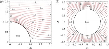
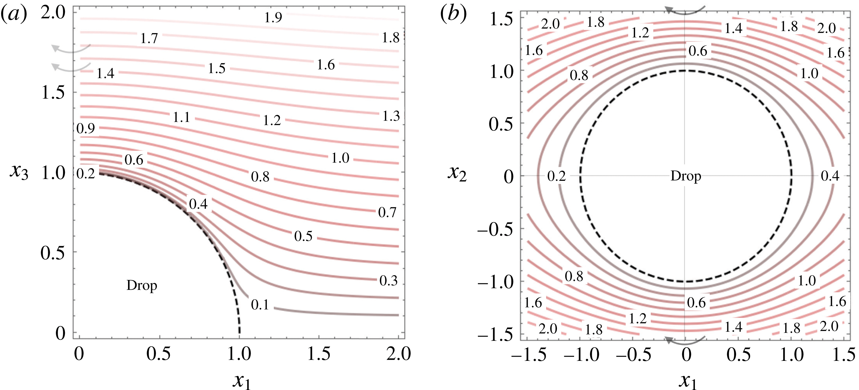
Projections of streamsurfaces of the external flow for the case of a drop in a linear flow with
 $\unicode[STIX]{x1D6FC}=0.2$
,
 $\unicode[STIX]{x1D706}=2$
. (a) Projections of the constant-
 $D$
surfaces on the (
 $x_{1},x_{3}$
) plane. These surfaces are surfaces of revolution about the
 $x_{3}$
axis as depicted by the curved arrows. (b) Projection of the near-field constant-
 $E$
surfaces on the (
 $x_{1},x_{2}$
) plane. These are surfaces of revolution about the
 $x_{2}$
axis as depicted by the curved arrows.
Thus, in the case of a drop, one needs to define a new radial coordinate which takes into account the radial displacements of the inertialess closed streamlines, displacements that, for the streamlines in the thermal boundary layer, are of the same order as the
 $O(RePe)^{-1/2}$
boundary layer thickness. Instead of spheres, as was the case for the solid particle and the drop in the open streamline regime (Krishnamurthy & Subramanian Reference Krishnamurthy and Subramanian2018), the streamsurfaces of the exterior Stokes flow serve as natural candidates for the constant coordinate surfaces, in the radial direction, in the closed streamline regime. These surfaces were originally identified by Cox et al. (Reference Cox, Zia and Mason1968) for a solid sphere in a simple shear flow, and were analysed in some detail for the case of a drop in Krishnamurthy & Subramanian (Reference Krishnamurthy and Subramanian2018). The streamsurfaces form two one-parameter families. The ones exterior to the drop, denoted as the constant-
 $D$
and
 $E$
surfaces therein, are surfaces of revolution about the
 $x_{3}$
and
 $x_{2}$
axes, respectively. It turns out that the drop surface (with or without the plane of symmetry
 $x_{3}=0$
) is itself a limiting streamsurface, corresponding to
 $D=0,E=0$
, for both families. Apart from indicating a degeneracy (near tangency) of the two families in the limit
 $r\rightarrow 1$
, this also leads to two possible choices for the (generalized) radial coordinate to be used in the boundary layer analysis. We choose the constant-
 $E$
surfaces (figure 4
b) to formulate the boundary layer analysis below. This is because these intersect transversally with the plane of symmetry, the curves of intersection being the in-plane Stokesian streamlines. In contrast, the constant-
 $D$
surfaces eventually become parallel to the plane of symmetry, approaching it at infinity for any
 $D>0$
(figure 4
a). Thus, although the near-field constant-
 $D$
surfaces would have their normal in the radial direction over most of the drop, they would eventually approach a tangential orientation sufficiently close to the plane of symmetry (figure 4
a), and this leads to a spurious dominance of tangential diffusion in this region.
In summary, one needs to move from an
 $(r,C,\unicode[STIX]{x1D70F})$
coordinate system to an
 $(E,C,\unicode[STIX]{x1D70F})$
system. This transformation need not be done exactly, since only the constant-
 $E$
surfaces in the thermal boundary layer matter, and these deviate from sphericity only by
 $O(RePe)^{-1/2}$
for large
 $RePe$
. We therefore derive the approximate near-field forms of the constant-
 $D$
and
 $E$
surfaces; the latter will be used in the large-
 $Pe$
analysis. The near-field Stokes velocity components in spherical coordinates are given by:
 $$\begin{eqnarray}\displaystyle & \displaystyle u_{r}=-{\displaystyle \frac{3(1+\unicode[STIX]{x1D6FC})}{1+\unicode[STIX]{x1D706}}}\sin ^{2}\unicode[STIX]{x1D703}\sin 2\unicode[STIX]{x1D719}_{1}y={\displaystyle \frac{\text{d}y}{\text{d}s}}, & \displaystyle\end{eqnarray}$$
 $$\begin{eqnarray}\displaystyle & \displaystyle u_{\unicode[STIX]{x1D703}}=-{\displaystyle \frac{(1+\unicode[STIX]{x1D6FC})}{2(1+\unicode[STIX]{x1D706})}}\sin 2\unicode[STIX]{x1D703}\sin 2\unicode[STIX]{x1D719}_{1}={\displaystyle \frac{\text{d}\unicode[STIX]{x1D703}}{\text{d}s}}, & \displaystyle\end{eqnarray}$$
 $$\begin{eqnarray}\displaystyle & \displaystyle u_{\unicode[STIX]{x1D719}}=-{\displaystyle \frac{(1+\unicode[STIX]{x1D6FC})}{1+\unicode[STIX]{x1D706}}}\sin \unicode[STIX]{x1D703}\left(\cos 2\unicode[STIX]{x1D719}_{1}+\unicode[STIX]{x1D6FD}\right)=\sin \unicode[STIX]{x1D703}{\displaystyle \frac{\text{d}\unicode[STIX]{x1D719}_{1}}{\text{d}s}}, & \displaystyle\end{eqnarray}$$
where
 $s$
denotes the time measured in units of inverse shear rate; recall that
 $\unicode[STIX]{x1D719}_{1}=\unicode[STIX]{x03C0}/2-\unicode[STIX]{x1D719}$
.
Dividing (2.23) by (2.24), one obtains:
 $$\begin{eqnarray}\displaystyle & \displaystyle {\displaystyle \frac{\text{d}y}{\text{d}\unicode[STIX]{x1D703}}}={\displaystyle \frac{3y\sin \unicode[STIX]{x1D703}}{\cos \unicode[STIX]{x1D703}}}. & \displaystyle\end{eqnarray}$$
Upon integrating this, the near-field form of the constant-
 $D$
surfaces, the parameter denoted here by
 $\unicode[STIX]{x1D713}$
, are given by:
 $$\begin{eqnarray}\displaystyle & \displaystyle \unicode[STIX]{x1D713}=\cos ^{3}\unicode[STIX]{x1D703}y. & \displaystyle\end{eqnarray}$$
Based on the known functional form of the constant-
 $D$
surfaces (Krishnamurthy & Subramanian Reference Krishnamurthy and Subramanian2018),
 $\unicode[STIX]{x1D713}$
and
 $D$
can be shown to be related as:
 $$\begin{eqnarray}\displaystyle & \displaystyle \unicode[STIX]{x1D713}=D^{3}\left[{\displaystyle \frac{3(\unicode[STIX]{x1D706}+2)}{2(\unicode[STIX]{x1D706}+1)}}\right]^{-1}. & \displaystyle\end{eqnarray}$$
Similarly, from (2.25) and (2.24), one obtains:
 $$\begin{eqnarray}\displaystyle & \displaystyle \sin \unicode[STIX]{x1D703}\cos \unicode[STIX]{x1D703}\sin 2\unicode[STIX]{x1D719}{\displaystyle \frac{\text{d}\unicode[STIX]{x1D719}}{\text{d}\unicode[STIX]{x1D703}}}=\cos 2\unicode[STIX]{x1D719}+\unicode[STIX]{x1D6FD}(1+\unicode[STIX]{x1D706}). & \displaystyle\end{eqnarray}$$
Upon rearranging, this becomes:
 $$\begin{eqnarray}\displaystyle & \displaystyle {\displaystyle \frac{\text{d}(\tan ^{2}\unicode[STIX]{x1D703}\cos ^{2}\unicode[STIX]{x1D719}_{1})}{\text{d}\unicode[STIX]{x1D703}}}=[1-\unicode[STIX]{x1D6FD}(1+\unicode[STIX]{x1D706})]{\displaystyle \frac{\sin \unicode[STIX]{x1D703}}{\cos ^{2}\unicode[STIX]{x1D703}}}. & \displaystyle\end{eqnarray}$$
Further, dividing (2.30) by (2.26), we get:
 $$\begin{eqnarray}\displaystyle & \displaystyle {\displaystyle \frac{\text{d}(\tan ^{2}\unicode[STIX]{x1D703}\cos ^{2}\unicode[STIX]{x1D719}_{1})}{\text{d}y}}={\displaystyle \frac{[1-\unicode[STIX]{x1D6FD}(1+\unicode[STIX]{x1D706})]}{\cos ^{2}\unicode[STIX]{x1D703}}}. & \displaystyle\end{eqnarray}$$
Integrating from
 $y_{m}$
to
 $y$
and substituting for
 $\cos \unicode[STIX]{x1D703}$
from (2.27), we have:
 $$\begin{eqnarray}\displaystyle & \displaystyle \int _{y_{m}}^{y}{\displaystyle \frac{\text{d}(\tan ^{2}\unicode[STIX]{x1D703}\cos ^{2}\unicode[STIX]{x1D719}_{1})}{\text{d}y}}\,\text{d}y={\displaystyle \frac{[1-\unicode[STIX]{x1D6FD}(1+\unicode[STIX]{x1D706})]}{3\unicode[STIX]{x1D713}^{2/3}}}\int _{y_{m}}^{y}y^{-1/3}, & \displaystyle\end{eqnarray}$$
where
 $y_{m}$
, which emerges as a constant of integration in the above analysis, is the new coordinate which characterizes the near-field inertialess streamlines. Imposing
 $\tan ^{2}\unicode[STIX]{x1D703}\cos ^{2}\unicode[STIX]{x1D719}_{1}=0$
at
 $y=y_{m}$
, one obtains after some algebra:
 $$\begin{eqnarray}\displaystyle & \displaystyle y_{m}=y\left[1-{\displaystyle \frac{2\sin ^{2}\unicode[STIX]{x1D703}\cos ^{2}\unicode[STIX]{x1D719}_{1}}{1-\unicode[STIX]{x1D6FD}(1+\unicode[STIX]{x1D706})}}\right]^{3/2}. & \displaystyle\end{eqnarray}$$
The constant-
 $y_{m}$
surfaces are the near-field forms of the constant-
 $E$
surfaces whose exact functional forms are given in Krishnamurthy & Subramanian (Reference Krishnamurthy and Subramanian2018), and have been derived earlier by Powell (Reference Powell1983). Writing (2.33) in terms of the
 $(C,\unicode[STIX]{x1D70F})$
coordinate system, the expression for the new radial coordinate is:
 $$\begin{eqnarray}\displaystyle & \displaystyle y_{m}=M(C,\unicode[STIX]{x1D70F})y, & \displaystyle\end{eqnarray}$$
where:
 $$\begin{eqnarray}\displaystyle & \displaystyle M(C,\unicode[STIX]{x1D70F})=\left[{\displaystyle \frac{1+C^{2}\unicode[STIX]{x1D6FE}^{2}}{1+C^{2}(\cos ^{2}\unicode[STIX]{x1D70F}+\unicode[STIX]{x1D6FE}^{2}\sin ^{2}\unicode[STIX]{x1D70F})}}\right]^{3/2}. & \displaystyle\end{eqnarray}$$
A near-field streamline is thus defined by a constant value of
 $y_{m}$
and
 $C$
,
 $y_{m}$
being a rescaled version of the original radial coordinate
 $y$
, equalling it when
 $\unicode[STIX]{x1D719}_{1}=\unicode[STIX]{x1D70F}=\unicode[STIX]{x03C0}/2$
. The scaling prefactor in (2.35) is a function of
 $C$
and
 $\unicode[STIX]{x1D70F}$
, and arises from the incompressibility constraint applied to an infinitesimal cylindrical fluid element, with its base on the drop. Specifically, the prefactor describes the change in height of such an element as a function of
 $\unicode[STIX]{x1D70F}$
as it moves along a Jeffery orbit (see figure 5). In the context of the boundary layer analysis that follows, it is worth reiterating that it is the constant-
 $y_{m}$
surfaces that are the near-field isotherms in the limit
 $Re=0$
,
 $Pe\rightarrow \infty$
, just as the constant-
 $y$
surfaces (spheres) were isotherms for a solid particle (Subramanian & Koch Reference Subramanian and Koch2006b
). The large-
 $Pe$
analysis below is implemented in the
 $(y_{m},C,\unicode[STIX]{x1D70F})$
coordinate system.
A schematic of a near-field Stokes streamline, corresponding to a constant-
 $y_{m}$
constant-
 $C$
curve, showing the varying radial distance from the drop surface. To satisfy the continuity constraint a fluid element moving along such a streamline has a height that is modulated by
 $M(C,\unicode[STIX]{x1D70F})$
.

2.4 The boundary layer analysis for
$Re\ll 1$
,
$RePe\gg 1$


Having characterized the radial coordinate required for the analysis, we now transform the convection–diffusion equation from the
 $(y,C,\unicode[STIX]{x1D70F})$
coordinate system to a
 $(y_{m},C,\unicode[STIX]{x1D70F})$
coordinate system. Using the chain rule for differentiation, one may write:
 $$\begin{eqnarray}\displaystyle & \displaystyle \left.{\displaystyle \frac{\unicode[STIX]{x2202}\unicode[STIX]{x1D6E9}}{\unicode[STIX]{x2202}y}}\right|_{C,\unicode[STIX]{x1D70F}}=\left.{\displaystyle \frac{\unicode[STIX]{x2202}\unicode[STIX]{x1D6E9}}{\unicode[STIX]{x2202}y_{m}}}\right|_{C,\unicode[STIX]{x1D70F}}\left.{\displaystyle \frac{\unicode[STIX]{x2202}y_{m}}{\unicode[STIX]{x2202}y}}\right|_{C,\unicode[STIX]{x1D70F}}, & \displaystyle\end{eqnarray}$$
 $$\begin{eqnarray}\displaystyle & \displaystyle \left.{\displaystyle \frac{\unicode[STIX]{x2202}\unicode[STIX]{x1D6E9}}{\unicode[STIX]{x2202}C}}\right|_{y,\unicode[STIX]{x1D70F}}=\left.{\displaystyle \frac{\unicode[STIX]{x2202}\unicode[STIX]{x1D6E9}}{\unicode[STIX]{x2202}y_{m}}}\right|_{C,\unicode[STIX]{x1D70F}}\left.{\displaystyle \frac{\unicode[STIX]{x2202}y_{m}}{\unicode[STIX]{x2202}C}}\right|_{y,\unicode[STIX]{x1D70F}}+\left.{\displaystyle \frac{\unicode[STIX]{x2202}\unicode[STIX]{x1D6E9}}{\unicode[STIX]{x2202}C}}\right|_{y_{m},\unicode[STIX]{x1D70F}}, & \displaystyle\end{eqnarray}$$
 $$\begin{eqnarray}\displaystyle & \displaystyle \left.{\displaystyle \frac{\unicode[STIX]{x2202}\unicode[STIX]{x1D6E9}}{\unicode[STIX]{x2202}\unicode[STIX]{x1D70F}}}\right|_{y,C}=\left.{\displaystyle \frac{\unicode[STIX]{x2202}\unicode[STIX]{x1D6E9}}{\unicode[STIX]{x2202}y_{m}}}\right|_{C,\unicode[STIX]{x1D70F}}\left.{\displaystyle \frac{\unicode[STIX]{x2202}y_{m}}{\unicode[STIX]{x2202}\unicode[STIX]{x1D70F}}}\right|_{y,C}+\left.{\displaystyle \frac{\unicode[STIX]{x2202}\unicode[STIX]{x1D6E9}}{\unicode[STIX]{x2202}\unicode[STIX]{x1D70F}}}\right|_{y_{m},C}. & \displaystyle\end{eqnarray}$$
The physical significance of (2.37) and (2.38) can be understood from figure 5. As one moves across Jeffery orbits (constant-
 $C$
curves) at a given
 $y$
, one ends up moving across constant-
 $y_{m}$
surfaces, and the consequent change in temperature corresponds to the first term in (2.37). A similar argument applies for the first term in (2.38). These terms therefore appear as additional ‘radial’ velocity contributions in the transformed convection–diffusion equation written below. For the derivative with respect to
 $y$
, however, the terms involving changes to the
 $C$
and
 $\unicode[STIX]{x1D70F}$
coordinates with respect to
 $y$
have been omitted. Such terms will, in general, be non-zero since the
 $(C,\unicode[STIX]{x1D70F})$
coordinate system is defined exactly at the drop surface, and the near-field closed streamlines are not exactly Jeffery orbits. For purposes of the boundary layer analysis, however, the perturbations to the
 $(C,\unicode[STIX]{x1D70F})$
coordinates are only
 $O(RePe)^{-1/2}$
.
Using the above expressions in (2.12), the convection–diffusion equation in the
 $(y_{m},C,\unicode[STIX]{x1D70F})$
coordinate system is given by:
 $$\begin{eqnarray}\displaystyle & \displaystyle \left(u_{r}{\displaystyle \frac{\unicode[STIX]{x2202}y_{m}}{\unicode[STIX]{x2202}y}}+{\displaystyle \frac{u_{C}}{h}}{\displaystyle \frac{\unicode[STIX]{x2202}y_{m}}{\unicode[STIX]{x2202}C}}+{\displaystyle \frac{u_{\unicode[STIX]{x1D70F}}}{k}}{\displaystyle \frac{\unicode[STIX]{x2202}y_{m}}{\unicode[STIX]{x2202}\unicode[STIX]{x1D70F}}}\right){\displaystyle \frac{\unicode[STIX]{x2202}\unicode[STIX]{x1D6E9}}{\unicode[STIX]{x2202}y_{m}}}+{\displaystyle \frac{u_{C}}{h}}\left.{\displaystyle \frac{\unicode[STIX]{x2202}\unicode[STIX]{x1D6E9}}{\unicode[STIX]{x2202}C}}\right|_{y_{m},\unicode[STIX]{x1D70F}}+{\displaystyle \frac{u_{\unicode[STIX]{x1D70F}}}{k}}\left.{\displaystyle \frac{\unicode[STIX]{x2202}\unicode[STIX]{x1D6E9}}{\unicode[STIX]{x2202}\unicode[STIX]{x1D70F}}}\right|_{y_{m},C}={\displaystyle \frac{1}{Pe}}\left({\displaystyle \frac{\unicode[STIX]{x2202}y_{m}}{\unicode[STIX]{x2202}y}}\right)^{2}{\displaystyle \frac{\unicode[STIX]{x2202}^{2}\unicode[STIX]{x1D6E9}}{\unicode[STIX]{x2202}y_{m}^{2}}}, & \displaystyle \nonumber\\ \displaystyle & & \displaystyle\end{eqnarray}$$
where each of the velocity components in (2.39) includes a Stokes and an
 $O(Re)$
contribution. We have anticipated the dominance of radial diffusion in the thermal boundary layer. The term
 $\left(\unicode[STIX]{x2202}y_{m}/\unicode[STIX]{x2202}y\right)^{2}$
captures the variation of the effective diffusivity which is larger in regions where the constant-
 $y_{m}$
surfaces (isotherms at zero
 $Re$
) are squeezed close together (
 $\unicode[STIX]{x2202}y_{m}/\unicode[STIX]{x2202}y>1$
) and smaller when they are further apart (
 $\unicode[STIX]{x2202}y_{m}/\unicode[STIX]{x2202}y<1$
).
Considering only the Stokes contributions to the convection terms, to begin with, one obtains:
 $$\begin{eqnarray}\displaystyle & \displaystyle \left(u_{r}^{(0)}{\displaystyle \frac{\unicode[STIX]{x2202}y_{m}}{\unicode[STIX]{x2202}y}}+{\displaystyle \frac{u_{C}^{(0)}}{h}}{\displaystyle \frac{\unicode[STIX]{x2202}y_{m}}{\unicode[STIX]{x2202}C}}+{\displaystyle \frac{u_{\unicode[STIX]{x1D70F}}^{(0)}}{k}}{\displaystyle \frac{\unicode[STIX]{x2202}y_{m}}{\unicode[STIX]{x2202}\unicode[STIX]{x1D70F}}}\right){\displaystyle \frac{\unicode[STIX]{x2202}\unicode[STIX]{x1D6E9}}{\unicode[STIX]{x2202}y_{m}}}+{\displaystyle \frac{u_{C}^{(0)}}{h}}{\displaystyle \frac{\unicode[STIX]{x2202}\unicode[STIX]{x1D6E9}}{\unicode[STIX]{x2202}C}}+{\displaystyle \frac{u_{\unicode[STIX]{x1D70F}}^{(0)}}{k}}{\displaystyle \frac{\unicode[STIX]{x2202}\unicode[STIX]{x1D6E9}}{\unicode[STIX]{x2202}\unicode[STIX]{x1D70F}}}={\displaystyle \frac{1}{Pe}}{\displaystyle \frac{\unicode[STIX]{x2202}^{2}\unicode[STIX]{x1D6E9}}{\unicode[STIX]{x2202}y_{m}^{2}}}\left({\displaystyle \frac{\unicode[STIX]{x2202}y_{m}}{\unicode[STIX]{x2202}y}}\right)^{2}, & \displaystyle \nonumber\\ \displaystyle & & \displaystyle\end{eqnarray}$$
where
 $u_{C}^{(0)}=0$
. Near the surface of the drop, using (2.16) and (2.19) the above equation becomes:
 $$\begin{eqnarray}\displaystyle & \displaystyle \left(h_{r}^{(0)}y{\displaystyle \frac{\unicode[STIX]{x2202}y_{m}}{\unicode[STIX]{x2202}y}}+h_{\unicode[STIX]{x1D70F}}^{(0)}{\displaystyle \frac{\unicode[STIX]{x2202}y_{m}}{\unicode[STIX]{x2202}\unicode[STIX]{x1D70F}}}\right){\displaystyle \frac{\unicode[STIX]{x2202}\unicode[STIX]{x1D6E9}}{\unicode[STIX]{x2202}y_{m}}}+h_{\unicode[STIX]{x1D70F}}^{(0)}{\displaystyle \frac{\unicode[STIX]{x2202}\unicode[STIX]{x1D6E9}}{\unicode[STIX]{x2202}\unicode[STIX]{x1D70F}}}={\displaystyle \frac{1}{Pe}}{\displaystyle \frac{\unicode[STIX]{x2202}^{2}\unicode[STIX]{x1D6E9}}{\unicode[STIX]{x2202}y_{m}^{2}}}\left({\displaystyle \frac{\unicode[STIX]{x2202}y_{m}}{\unicode[STIX]{x2202}y}}\right)^{2}. & \displaystyle\end{eqnarray}$$
Further, since:
 $$\begin{eqnarray}\displaystyle & \displaystyle h_{r}^{(0)}y{\displaystyle \frac{\unicode[STIX]{x2202}y_{m}}{\unicode[STIX]{x2202}y}}+h_{\unicode[STIX]{x1D70F}}^{(0)}{\displaystyle \frac{\unicode[STIX]{x2202}y_{m}}{\unicode[STIX]{x2202}\unicode[STIX]{x1D70F}}}=0, & \displaystyle\end{eqnarray}$$
the rate of convection in the
 $y_{m}$
direction vanishes, This is simply a mathematical statement of the fact that the Stokes velocity field, by definition, cannot lead to convection across constant-
 $y_{m}$
surfaces, which are the invariant Stokes streamsurfaces. Thus, at leading order, in the limit of
 $Pe\gg 1$
, one has:
 $$\begin{eqnarray}\displaystyle & \displaystyle \left.{\displaystyle \frac{\unicode[STIX]{x2202}\unicode[STIX]{x1D6E9}^{(0)}}{\unicode[STIX]{x2202}\unicode[STIX]{x1D70F}}}\right|_{y_{m},C}=0, & \displaystyle\end{eqnarray}$$
which implies that the leading-order temperature field is independent of
 $\unicode[STIX]{x1D70F}$
at steady state. The transformation to the new radial coordinate has helped one directly see the isothermality of the closed Stokesian streamlines.
Expand the temperature field, for small but finite
 $Re$
, as:
 $$\begin{eqnarray}\displaystyle & \displaystyle \unicode[STIX]{x1D6E9}=\unicode[STIX]{x1D6E9}^{(0)}(y_{m},C)+F(Re,Pe)\unicode[STIX]{x1D6E9}^{(1)}(y_{m},C,\unicode[STIX]{x1D70F}), & \displaystyle\end{eqnarray}$$
where
 $F(Re,Pe)$
is a small parameter, and will turn out to be proportional to the boundary layer thickness. Writing the convection–diffusion equation, with the velocity field now written down to
 $O(Re)$
, and making use of (2.42) and (2.43), one obtains:
 $$\begin{eqnarray}\displaystyle & & \displaystyle \displaystyle \left(Reu_{r}^{(1)}{\displaystyle \frac{\unicode[STIX]{x2202}y_{m}}{\unicode[STIX]{x2202}y}}+Re{\displaystyle \frac{u_{C}^{(1)}}{h}}{\displaystyle \frac{\unicode[STIX]{x2202}y_{m}}{\unicode[STIX]{x2202}C}}+Re{\displaystyle \frac{u_{\unicode[STIX]{x1D70F}}^{(1)}}{k}}{\displaystyle \frac{\unicode[STIX]{x2202}y_{m}}{\unicode[STIX]{x2202}\unicode[STIX]{x1D70F}}}\right){\displaystyle \frac{\unicode[STIX]{x2202}\unicode[STIX]{x1D6E9}^{(0)}}{\unicode[STIX]{x2202}y_{m}}}+Re{\displaystyle \frac{u_{C}^{(1)}}{h}}{\displaystyle \frac{\unicode[STIX]{x2202}\unicode[STIX]{x1D6E9}^{(0)}}{\unicode[STIX]{x2202}C}}\nonumber\\ \displaystyle & & \displaystyle \quad +\,Ref(Re,Pe){\displaystyle \frac{u_{\unicode[STIX]{x1D70F}}^{(0)}}{k}}{\displaystyle \frac{\unicode[STIX]{x2202}\unicode[STIX]{x1D6E9}^{(1)}}{\unicode[STIX]{x2202}\unicode[STIX]{x1D70F}}}={\displaystyle \frac{1}{Pe}}{\displaystyle \frac{\unicode[STIX]{x2202}^{2}\unicode[STIX]{x1D6E9}^{(0)}}{\unicode[STIX]{x2202}y_{m}^{2}}}\left({\displaystyle \frac{\unicode[STIX]{x2202}y_{m}}{\unicode[STIX]{x2202}y}}\right)^{2}.\end{eqnarray}$$
Since
 $u_{\unicode[STIX]{x1D70F}}^{(0)}/k$
is a constant, one may average the above equation over the Stokesian surface streamlines. This is equivalent to an integration over
 $\unicode[STIX]{x1D70F}$
from
 $0$
to
 $2\unicode[STIX]{x03C0}$
, which eliminates the term involving
 $\unicode[STIX]{x1D6E9}^{(1)}$
, and one obtains the
 $\unicode[STIX]{x1D70F}$
-averaged equation that governs the leading-order boundary layer temperature field
 $\unicode[STIX]{x1D6E9}^{(0)}$
:
 $$\begin{eqnarray}\displaystyle & & \displaystyle \displaystyle Re\left[\int _{0}^{2\unicode[STIX]{x03C0}}\left(u_{r}^{(1)}{\displaystyle \frac{\unicode[STIX]{x2202}y_{m}}{\unicode[STIX]{x2202}y}}+{\displaystyle \frac{u_{C}^{(1)}}{h}}{\displaystyle \frac{\unicode[STIX]{x2202}y_{m}}{\unicode[STIX]{x2202}C}}+{\displaystyle \frac{u_{\unicode[STIX]{x1D70F}}^{(1)}}{k}}{\displaystyle \frac{\unicode[STIX]{x2202}y_{m}}{\unicode[STIX]{x2202}\unicode[STIX]{x1D70F}}}\right)\text{d}\unicode[STIX]{x1D70F}\right]{\displaystyle \frac{\unicode[STIX]{x2202}\unicode[STIX]{x1D6E9}^{(0)}}{\unicode[STIX]{x2202}y_{m}}}\nonumber\\ \displaystyle & & \displaystyle \quad +\,Re\left[\int _{0}^{2\unicode[STIX]{x03C0}}\left({\displaystyle \frac{u_{C}^{(1)}}{h}}\right)\text{d}\unicode[STIX]{x1D70F}\right]{\displaystyle \frac{\unicode[STIX]{x2202}\unicode[STIX]{x1D6E9}^{(0)}}{\unicode[STIX]{x2202}C}}={\displaystyle \frac{1}{Pe}}\left[\int _{0}^{2\unicode[STIX]{x03C0}}\left({\displaystyle \frac{\unicode[STIX]{x2202}y_{m}}{\unicode[STIX]{x2202}y}}\right)^{2}\,\text{d}\unicode[STIX]{x1D70F}\right]{\displaystyle \frac{\unicode[STIX]{x2202}^{2}\unicode[STIX]{x1D6E9}^{(0)}}{\unicode[STIX]{x2202}y_{m}^{2}}}.\end{eqnarray}$$
Expanding the inertial velocity components in the near field using (2.20)–(2.22), one obtains:
 $$\begin{eqnarray}\displaystyle & & \displaystyle \displaystyle \left[\int _{0}^{2\unicode[STIX]{x03C0}}\left(h_{r}^{(1)}y{\displaystyle \frac{\unicode[STIX]{x2202}y_{m}}{\unicode[STIX]{x2202}y}}+h_{C}^{(1)}{\displaystyle \frac{\unicode[STIX]{x2202}y_{m}}{\unicode[STIX]{x2202}C}}+h_{\unicode[STIX]{x1D70F}}^{(1)}{\displaystyle \frac{\unicode[STIX]{x2202}y_{m}}{\unicode[STIX]{x2202}\unicode[STIX]{x1D70F}}}\right)\text{d}\unicode[STIX]{x1D70F}\right]{\displaystyle \frac{\unicode[STIX]{x2202}\unicode[STIX]{x1D6E9}^{(0)}}{\unicode[STIX]{x2202}y_{m}}}\nonumber\\ \displaystyle & & \displaystyle \quad +\,\left[\int _{0}^{2\unicode[STIX]{x03C0}}h_{C}^{(1)}\,\text{d}\unicode[STIX]{x1D70F}\right]{\displaystyle \frac{\unicode[STIX]{x2202}\unicode[STIX]{x1D6E9}^{(0)}}{\unicode[STIX]{x2202}C}}={\displaystyle \frac{1}{RePe}}\left[\int _{0}^{2\unicode[STIX]{x03C0}}\left({\displaystyle \frac{\unicode[STIX]{x2202}y_{m}}{\unicode[STIX]{x2202}y}}\right)^{2}\,\text{d}\unicode[STIX]{x1D70F}\right]{\displaystyle \frac{\unicode[STIX]{x2202}^{2}\unicode[STIX]{x1D6E9}^{(0)}}{\unicode[STIX]{x2202}y_{m}^{2}}}.\end{eqnarray}$$
In (2.47),
 $RePe$
naturally emerges as the parameter that governs the relative magnitudes of convection and diffusion. The
 $\unicode[STIX]{x1D70F}$
average used points to a crucial difference between the particle and drop cases. For the rotating particle, the uniform angular velocity implies that the inertial drift is uniformly averaged over
 $\unicode[STIX]{x1D719}$
. For a drop, the weighting is not uniform owing to the non-trivial relation between
 $\unicode[STIX]{x1D70F}$
and
 $\unicode[STIX]{x1D719}$
(see (2.7)). Interpreted as an average over
 $\unicode[STIX]{x1D719}$
, the parts of the orbit where the fluid elements are moving slower have a greater contribution to the
 $\unicode[STIX]{x1D70F}$
-averaged convection in (2.47) since inertia, acting over a longer time, leads to a greater drift in this regions; and vice versa.
It is worth mentioning that the simplicity of the leading-order equation, (2.43), belies the non-trivial approach towards
 $\unicode[STIX]{x1D70F}$
-independence via a shear-enhanced diffusion mechanism. In dimensional terms, equation (2.43) holds true for times much longer than
 $O(Pe^{-2/3})a^{2}/D$
, and this time scale is shorter than the time of
 $O([(RePe)^{-1/2}]^{2})a^{2}/D$
for inertia to set up a steady temperature field in the thermal boundary layer, provided
 $Re\ll Pe^{-1/3}$
. Thus, for
 $Re\ll Pe^{-1/3}$
, the evolution towards the steady state boundary layer temperature field satisfying (2.47) would proceed through an intermediate asymptotic stage when the Jeffery-orbit-like turns of the near-surface streamlines become nearly isothermal due to shear-enhanced diffusion, but with the temperature variation across the turns still being closely related to the initial field. When
 $Pe^{-1/3}\ll Re\ll 1$
, there is no separation of time scales between the (Stokesian) isothermalization and inertial convection. Since the tight spiralling of the inertial streamlines continues to hold, the
 $\unicode[STIX]{x1D70F}$
-averaging above may still be carried out to determine the boundary layer temperature field. For a solid particle, the tight spiralling of the inertial streamlines holds even when
 $Re$
is of order unity provided
 $Pe\gg 1$
, owing to the near-surface convecting velocity becoming weak (of
 $O(Pe)^{-1/3}$
) due to the no-slip boundary condition; this implies that a
 $\unicode[STIX]{x1D719}$
-averaged analysis may be carried out even when
 $Re$
is of order unity (Yang et al.
Reference Yang, Zhang, Koch and Yin2011). The
 $\unicode[STIX]{x1D70F}$
-averaging approach is, however, no longer valid when the drop
 $Re$
is of order unity.
From (2.47), it is clear that the scale for the boundary layer thickness is
 $O(Re^{-1/2}Pe^{-1/2})$
. Indeed, on postulating a rescaling for the modified radial coordinate
 $y_{m}$
of the form
 $Y_{m}=m(Re,Pe)y_{m}$
, where
 $Y_{m}$
is
 $O(1)$
, the leading-order balance gives
 $m(Re,Pe)=Re^{1/2}Pe^{1/2}$
. In terms of this rescaled coordinate, the
 $\unicode[STIX]{x1D70F}$
-averaged convection–diffusion equation is given by:
 $$\begin{eqnarray}\displaystyle & & \displaystyle \displaystyle \left[\int _{0}^{2\unicode[STIX]{x03C0}}\left(h_{r}^{(1)}Y_{m}+h_{C}^{(1)}{\displaystyle \frac{\unicode[STIX]{x2202}Y_{m}}{\unicode[STIX]{x2202}C}}+h_{\unicode[STIX]{x1D70F}}^{(1)}{\displaystyle \frac{\unicode[STIX]{x2202}Y_{m}}{\unicode[STIX]{x2202}\unicode[STIX]{x1D70F}}}\right)\text{d}\unicode[STIX]{x1D70F}\right]{\displaystyle \frac{\unicode[STIX]{x2202}\unicode[STIX]{x1D6E9}^{(0)}}{\unicode[STIX]{x2202}Y_{m}}}+\left[\int _{0}^{2\unicode[STIX]{x03C0}}h_{C}^{(1)}\,\text{d}\unicode[STIX]{x1D70F}\right]{\displaystyle \frac{\unicode[STIX]{x2202}\unicode[STIX]{x1D6E9}^{(0)}}{\unicode[STIX]{x2202}C}}\nonumber\\ \displaystyle & & \displaystyle \quad =\left[\int _{0}^{2\unicode[STIX]{x03C0}}\left({\displaystyle \frac{\unicode[STIX]{x2202}Y_{m}}{\unicode[STIX]{x2202}Y}}\right)^{2}\,\text{d}\unicode[STIX]{x1D70F}\right]{\displaystyle \frac{\unicode[STIX]{x2202}^{2}\unicode[STIX]{x1D6E9}^{(0)}}{\unicode[STIX]{x2202}Y_{m}^{2}}},\end{eqnarray}$$
where
 $Y_{m}$
and
 $Y$
are still related by (2.34). Using (2.33) the above equation can be rewritten as:
 $$\begin{eqnarray}\displaystyle & & \displaystyle \displaystyle Y_{m}\left[\int _{0}^{2\unicode[STIX]{x03C0}}\left(h_{r}^{(1)}+{\displaystyle \frac{h_{C}^{(1)}}{M}}{\displaystyle \frac{\unicode[STIX]{x2202}M}{\unicode[STIX]{x2202}C}}+{\displaystyle \frac{h_{\unicode[STIX]{x1D70F}}^{(1)}}{M}}{\displaystyle \frac{\unicode[STIX]{x2202}M}{\unicode[STIX]{x2202}\unicode[STIX]{x1D70F}}}\right)\text{d}\unicode[STIX]{x1D70F}\right]{\displaystyle \frac{\unicode[STIX]{x2202}\unicode[STIX]{x1D6E9}^{(0)}}{\unicode[STIX]{x2202}Y_{m}}}+\left[\int _{0}^{2\unicode[STIX]{x03C0}}h_{C}^{(1)}\,\text{d}\unicode[STIX]{x1D70F}\right]{\displaystyle \frac{\unicode[STIX]{x2202}\unicode[STIX]{x1D6E9}^{(0)}}{\unicode[STIX]{x2202}C}}\nonumber\\ \displaystyle & & \displaystyle \quad =\left[\int _{0}^{2\unicode[STIX]{x03C0}}\left({\displaystyle \frac{\unicode[STIX]{x2202}Y_{m}}{\unicode[STIX]{x2202}Y}}\right)^{2}\,\text{d}\unicode[STIX]{x1D70F}\right]{\displaystyle \frac{\unicode[STIX]{x2202}^{2}\unicode[STIX]{x1D6E9}^{(0)}}{\unicode[STIX]{x2202}Y_{m}^{2}}},\end{eqnarray}$$
which is of the form:
 $$\begin{eqnarray}\displaystyle & \displaystyle Y_{m}{\mathcal{A}}(C){\displaystyle \frac{\unicode[STIX]{x2202}\unicode[STIX]{x1D6E9}^{(0)}}{\unicode[STIX]{x2202}Y_{m}}}+{\mathcal{B}}(C){\displaystyle \frac{\unicode[STIX]{x2202}\unicode[STIX]{x1D6E9}^{(0)}}{\unicode[STIX]{x2202}C}}={\mathcal{D}}(C){\displaystyle \frac{\unicode[STIX]{x2202}^{2}\unicode[STIX]{x1D6E9}^{(0)}}{\unicode[STIX]{x2202}Y_{m}^{2}}}, & \displaystyle\end{eqnarray}$$
where
 $$\begin{eqnarray}\displaystyle \displaystyle {\mathcal{A}}(C) & = & \displaystyle \int _{0}^{2\unicode[STIX]{x03C0}}\left(h_{r}^{(1)}+{\displaystyle \frac{h_{C}^{(1)}}{M}}{\displaystyle \frac{\unicode[STIX]{x2202}M}{\unicode[STIX]{x2202}C}}+{\displaystyle \frac{h_{\unicode[STIX]{x1D70F}}^{(1)}}{M}}{\displaystyle \frac{\unicode[STIX]{x2202}M}{\unicode[STIX]{x2202}\unicode[STIX]{x1D70F}}}\right)\text{d}\unicode[STIX]{x1D70F},\end{eqnarray}$$
 $$\begin{eqnarray}\displaystyle \displaystyle {\mathcal{B}}(C) & = & \displaystyle \int _{0}^{2\unicode[STIX]{x03C0}}h_{C}^{(1)}\,\text{d}\unicode[STIX]{x1D70F},\end{eqnarray}$$
 $$\begin{eqnarray}\displaystyle \displaystyle {\mathcal{D}}(C) & = & \displaystyle \int _{0}^{2\unicode[STIX]{x03C0}}\left({\displaystyle \frac{\unicode[STIX]{x2202}Y_{m}}{\unicode[STIX]{x2202}Y}}\right)^{2}\,\text{d}\unicode[STIX]{x1D70F},\end{eqnarray}$$
 $$\begin{eqnarray}\displaystyle & = & \displaystyle {\displaystyle \frac{\unicode[STIX]{x03C0}\sqrt{1+C^{2}\unicode[STIX]{x1D6FE}^{2}}\left(8+8C^{2}\left(1+\unicode[STIX]{x1D6FE}^{2}\right)+C^{4}\left(3+2\unicode[STIX]{x1D6FE}^{2}+3\unicode[STIX]{x1D6FE}^{4}\right)\right)}{4\left(1+C^{2}\right)^{5/2}}}.\end{eqnarray}$$
The detailed closed-form expression for
 ${\mathcal{B}}(C)$
is given in appendix C, and that for
 ${\mathcal{A}}(C)$
may be obtained using a relation derived below (see (2.71)).
Note that the original three-dimensional non-axisymmetric heat transfer problem at small but finite
 $Re$
has been reduced, through the use of an appropriate coordinate system and phase averaging over the inertialess closed streamlines, to one resembling an axisymmetric problem, where the tangential convection is along a single coordinate (
 $C$
). The physical interpretations of the three factors
 ${\mathcal{A}}(C)$
,
 ${\mathcal{B}}(C)$
and
 ${\mathcal{D}}(C)$
follow naturally.
 ${\mathcal{A}}(C)$
represents the convective flux across the constant-
 $y_{m}$
surfaces due to the
 $\unicode[STIX]{x1D70F}$
-averaged inertial velocity field.
 ${\mathcal{B}}(C)$
represents the
 $\unicode[STIX]{x1D70F}$
-averaged convective flux tangential to the drop surface. The thermal wake must therefore correspond to the
 $C$
- location (implying that the wake is a Jeffery orbit to the order considered) at which this tangential convection vanishes.
 ${\mathcal{D}}(C)$
is the ‘orbit-dependent diffusivity’ which is the original constant molecular diffusivity (
 $1/Pe$
in non-dimensional terms) modulated by the spacing of the near-field Stokesian streamsurfaces.
One now introduces a similarity variable of the form
 $\unicode[STIX]{x1D702}=Y_{m}/g(C)$
, where
 $g(C)$
characterizes the dependence of the
 $\unicode[STIX]{x1D70F}$
-averaged boundary layer thickness as a function of position on the drop surface. Unlike the open streamline regime examined in Krishnamurthy & Subramanian (Reference Krishnamurthy and Subramanian2018), the boundary layer thickness on account of
 $\unicode[STIX]{x1D70F}$
-averaging is only a function of
 $C$
. Transforming (2.50), the non-dimensional temperature field satisfies:
 $$\begin{eqnarray}\displaystyle & \displaystyle {\displaystyle \frac{\text{d}^{2}\unicode[STIX]{x1D6E9}}{\text{d}\unicode[STIX]{x1D702}^{2}}}+2\unicode[STIX]{x1D702}{\displaystyle \frac{\text{d}\unicode[STIX]{x1D6E9}}{\text{d}\unicode[STIX]{x1D702}}}=0, & \displaystyle\end{eqnarray}$$
with the boundary layer thickness governed by:
 $$\begin{eqnarray}\displaystyle & \displaystyle {\displaystyle \frac{\text{d}f}{\text{d}C}}-{\displaystyle \frac{2{\mathcal{A}}(C)}{{\mathcal{B}}(C)}}f={\displaystyle \frac{2{\mathcal{D}}(C)}{{\mathcal{B}}(C)}}, & \displaystyle\end{eqnarray}$$
where
 $f=g^{2}/2$
. The boundary conditions for the non-dimensional temperature are:
 $$\begin{eqnarray}\displaystyle & \displaystyle \unicode[STIX]{x1D6E9}=1\quad \text{at}~\unicode[STIX]{x1D702}=0, & \displaystyle\end{eqnarray}$$
 $$\begin{eqnarray}\displaystyle & \displaystyle \unicode[STIX]{x1D6E9}\rightarrow 0\quad \text{as}~\unicode[STIX]{x1D702}\rightarrow \infty . & \displaystyle\end{eqnarray}$$
Solving (2.55) and using (2.57) and (2.58):
 $$\begin{eqnarray}\displaystyle & \displaystyle \unicode[STIX]{x1D6E9}(\unicode[STIX]{x1D702})=1-{\displaystyle \frac{2}{\sqrt{\unicode[STIX]{x03C0}}}}\int _{0}^{\unicode[STIX]{x1D702}}\exp (-t^{2})\,\text{d}t. & \displaystyle\end{eqnarray}$$
In order to solve for the boundary layer thickness profile from (2.56), without tedious algebraic manipulation, and thence calculate
 $Nu$
, it helps to relate the
 $\unicode[STIX]{x1D70F}$
-averaged radial (
 ${\mathcal{A}}(C)$
) and tangential (
 ${\mathcal{B}}(C)$
) velocities. Such a relation is immediate in simpler problems, but here one starts from the continuity equation for the Stokes velocity field, written in
 $(y,C,\unicode[STIX]{x1D70F})$
coordinates:
 $$\begin{eqnarray}\displaystyle & \displaystyle {\displaystyle \frac{\unicode[STIX]{x2202}(hk\sin \unicode[STIX]{x1D6FC}_{1}u_{r}^{(0)})}{\unicode[STIX]{x2202}y}}+{\displaystyle \frac{\unicode[STIX]{x2202}(k\sin \unicode[STIX]{x1D6FC}_{1}u_{C}^{(0)})}{\unicode[STIX]{x2202}C}}+{\displaystyle \frac{\unicode[STIX]{x2202}(h\sin \unicode[STIX]{x1D6FC}_{1}u_{\unicode[STIX]{x1D70F}}^{(0)})}{\unicode[STIX]{x2202}\unicode[STIX]{x1D70F}}}=0, & \displaystyle\end{eqnarray}$$
where
 $u_{C}^{(0)}=0$
, as before, by definition. In terms of the velocity field near the drop surface, the remaining two terms take the form:
 $$\begin{eqnarray}\displaystyle & \displaystyle {\displaystyle \frac{\unicode[STIX]{x2202}(hk\sin \unicode[STIX]{x1D6FC}_{1}h_{r}^{(0)}y)}{\unicode[STIX]{x2202}y}}+{\displaystyle \frac{\unicode[STIX]{x2202}(hk\sin \unicode[STIX]{x1D6FC}_{1}h_{\unicode[STIX]{x1D70F}}^{(0)})}{\unicode[STIX]{x2202}\unicode[STIX]{x1D70F}}}=0. & \displaystyle\end{eqnarray}$$
Noting that
 $h_{\unicode[STIX]{x1D70F}}^{(0)}$
is independent of both
 $C$
and
 $\unicode[STIX]{x1D70F}$
and that the combination of metric factors
 $hk\sin \unicode[STIX]{x1D6FC}_{1}$
(the area of an elementary parallelogram) is independent of the radial coordinate at leading order, one can write the above equation as:
 $$\begin{eqnarray}\displaystyle & \displaystyle hk\sin \unicode[STIX]{x1D6FC}_{1}h_{r}^{(0)}+h_{\unicode[STIX]{x1D70F}}^{(0)}{\displaystyle \frac{\unicode[STIX]{x2202}(hk\sin \unicode[STIX]{x1D6FC}_{1})}{\unicode[STIX]{x2202}\unicode[STIX]{x1D70F}}}=0. & \displaystyle\end{eqnarray}$$
From (2.33) and (2.42), the radial Stokes velocity measure,
 $h_{r}^{(0)}$
, may be written as:
 $$\begin{eqnarray}\displaystyle & \displaystyle h_{r}^{(0)}=-{\displaystyle \frac{1}{M}}{\displaystyle \frac{\unicode[STIX]{x2202}M}{\unicode[STIX]{x2202}\unicode[STIX]{x1D70F}}}h_{\unicode[STIX]{x1D70F}}^{(0)}, & \displaystyle\end{eqnarray}$$
where
 $M(C,\unicode[STIX]{x1D70F})$
is given by (2.35). Substituting for
 $h_{r}^{(0)}$
in (2.62), one has the relation:
 $$\begin{eqnarray}\displaystyle & \displaystyle {\displaystyle \frac{1}{M}}{\displaystyle \frac{\unicode[STIX]{x2202}M}{\unicode[STIX]{x2202}\unicode[STIX]{x1D70F}}}={\displaystyle \frac{1}{hk\sin \unicode[STIX]{x1D6FC}_{1}}}{\displaystyle \frac{\unicode[STIX]{x2202}(hk\sin \unicode[STIX]{x1D6FC}_{1})}{\unicode[STIX]{x2202}\unicode[STIX]{x1D70F}}}. & \displaystyle\end{eqnarray}$$
This is the statement of volume conservation applied to a cylindrical fluid element as it moves along an inertialess Stokes orbit, with its base on the surface of the spherical drop (see figure 5). The volume of such an infinitesimal fluid element is given by
 $\unicode[STIX]{x0394}V=hk\sin \unicode[STIX]{x1D6FC}_{1}\unicode[STIX]{x0394}C\unicode[STIX]{x0394}\unicode[STIX]{x1D70F}y_{m}/M(C,\unicode[STIX]{x1D70F})$
and the above equation is then the same as the condition that
 $\unicode[STIX]{x2202}(\unicode[STIX]{x0394}V)/\unicode[STIX]{x2202}\unicode[STIX]{x1D70F}|_{y_{m},C}=0$
.
Next, the continuity equation, at
 $O(Re)$
expressed in
 $(y,C,\unicode[STIX]{x1D70F})$
coordinates is given by:
 $$\begin{eqnarray}\displaystyle & \displaystyle hk\sin \unicode[STIX]{x1D6FC}_{1}{\displaystyle \frac{\unicode[STIX]{x2202}u_{r}^{(1)}}{\unicode[STIX]{x2202}y}}+{\displaystyle \frac{\unicode[STIX]{x2202}(k\sin \unicode[STIX]{x1D6FC}_{1}u_{C}^{(1)})}{\unicode[STIX]{x2202}C}}+{\displaystyle \frac{\unicode[STIX]{x2202}(h\sin \unicode[STIX]{x1D6FC}_{1}u_{\unicode[STIX]{x1D70F}}^{(1)})}{\unicode[STIX]{x2202}\unicode[STIX]{x1D70F}}}=0. & \displaystyle\end{eqnarray}$$
Rewriting this equation for the near-field inertial velocity, one has:
 $$\begin{eqnarray}\displaystyle & \displaystyle h_{r}^{(1)}+{\displaystyle \frac{1}{hk\sin \unicode[STIX]{x1D6FC}_{1}}}{\displaystyle \frac{\unicode[STIX]{x2202}(hk\sin \unicode[STIX]{x1D6FC}_{1}h_{C}^{(1)})}{\unicode[STIX]{x2202}C}}+{\displaystyle \frac{1}{hk\sin \unicode[STIX]{x1D6FC}_{1}}}{\displaystyle \frac{\unicode[STIX]{x2202}(hk\sin \unicode[STIX]{x1D6FC}_{1}h_{\unicode[STIX]{x1D70F}}^{(1)})}{\unicode[STIX]{x2202}\unicode[STIX]{x1D70F}}}=0. & \displaystyle\end{eqnarray}$$
Expanding the last term and using the relation (2.64), one obtains:
 $$\begin{eqnarray}\displaystyle & \displaystyle h_{r}^{(1)}+{\displaystyle \frac{h_{\unicode[STIX]{x1D70F}}^{(1)}}{M}}{\displaystyle \frac{\unicode[STIX]{x2202}M}{\unicode[STIX]{x2202}\unicode[STIX]{x1D70F}}}=-\left[{\displaystyle \frac{\unicode[STIX]{x2202}h_{\unicode[STIX]{x1D70F}}^{(1)}}{\unicode[STIX]{x2202}\unicode[STIX]{x1D70F}}}+{\displaystyle \frac{1}{hk\sin \unicode[STIX]{x1D6FC}_{1}}}{\displaystyle \frac{\unicode[STIX]{x2202}(hk\sin \unicode[STIX]{x1D6FC}_{1}h_{C}^{(1)})}{\unicode[STIX]{x2202}C}}\right]. & \displaystyle\end{eqnarray}$$
Note that the left-hand side of the above equation contains the first and third terms in the integrand in the expression for
 ${\mathcal{A}}(C)$
(see (2.51)). Upon substitution, one gets:
 $$\begin{eqnarray}\displaystyle & \displaystyle {\mathcal{A}}(C)=\int _{0}^{2\unicode[STIX]{x03C0}}\left[-{\displaystyle \frac{\unicode[STIX]{x2202}h_{\unicode[STIX]{x1D70F}}^{(1)}}{\unicode[STIX]{x2202}\unicode[STIX]{x1D70F}}}-{\displaystyle \frac{1}{hk\sin \unicode[STIX]{x1D6FC}_{1}}}{\displaystyle \frac{\unicode[STIX]{x2202}(hk\sin \unicode[STIX]{x1D6FC}_{1}h_{C}^{(1)})}{\unicode[STIX]{x2202}C}}+{\displaystyle \frac{h_{C}^{(1)}}{M}}{\displaystyle \frac{\unicode[STIX]{x2202}M}{\unicode[STIX]{x2202}C}}\right]\text{d}\unicode[STIX]{x1D70F}. & \displaystyle\end{eqnarray}$$
The first term in the above expression is an exact differential, and hence zero when integrated from
 $0$
to
 $2\unicode[STIX]{x03C0}$
. Upon rearranging the expression further, one has:
 $$\begin{eqnarray}\displaystyle & \displaystyle {\mathcal{A}}(C)=\int _{0}^{2\unicode[STIX]{x03C0}}\left[\left({\displaystyle \frac{1}{M}}{\displaystyle \frac{\unicode[STIX]{x2202}M}{\unicode[STIX]{x2202}C}}-{\displaystyle \frac{1}{hk\sin \unicode[STIX]{x1D6FC}_{1}}}{\displaystyle \frac{\unicode[STIX]{x2202}(hk\sin \unicode[STIX]{x1D6FC}_{1})}{\unicode[STIX]{x2202}C}}\right)h_{C}^{(1)}-{\displaystyle \frac{\unicode[STIX]{x2202}h_{C}^{(1)}}{\unicode[STIX]{x2202}C}}\right]\text{d}\unicode[STIX]{x1D70F}. & \displaystyle\end{eqnarray}$$
Since the term:
 $$\begin{eqnarray}\displaystyle & \displaystyle {\displaystyle \frac{1}{M}}{\displaystyle \frac{\unicode[STIX]{x2202}M}{\unicode[STIX]{x2202}C}}-{\displaystyle \frac{1}{hk\sin \unicode[STIX]{x1D6FC}_{1}}}{\displaystyle \frac{\unicode[STIX]{x2202}(hk\sin \unicode[STIX]{x1D6FC}_{1})}{\unicode[STIX]{x2202}C}}={\displaystyle \frac{2C^{2}\unicode[STIX]{x1D6FE}^{2}-1}{C(1+C^{2}\unicode[STIX]{x1D6FE}^{2})}}, & \displaystyle\end{eqnarray}$$
which is independent of
 $\unicode[STIX]{x1D70F}$
and can therefore be pulled out of the integral, the remaining terms can be expressed in terms of
 ${\mathcal{B}}(C)$
, giving the final relation between
 ${\mathcal{A}}(C)$
and
 ${\mathcal{B}}(C)$
as:
 $$\begin{eqnarray}\displaystyle & \displaystyle {\mathcal{A}}(C)={\displaystyle \frac{2C^{2}\unicode[STIX]{x1D6FE}^{2}-1}{C(1+C^{2}\unicode[STIX]{x1D6FE}^{2})}}{\mathcal{B}}(C)-{\displaystyle \frac{\text{d}{\mathcal{B}}(C)}{\text{d}C}}. & \displaystyle\end{eqnarray}$$
The above expression is a statement of the
 $\unicode[STIX]{x1D70F}$
-averaged continuity equation for the
 $O(Re)$
velocity field. The
 $\unicode[STIX]{x1D70F}$
averaging trivially excludes any convection in the
 $\unicode[STIX]{x1D70F}$
direction, even at
 $O(Re)$
, which leaves only the convection in the radial (across constant-
 $y_{m}$
surfaces) and
 $C$
directions (across Jeffery orbits) denoted by
 ${\mathcal{A}}(C)$
and
 ${\mathcal{B}}(C)$
, respectively. The continuity equation dictates that these two must be related and the relation is given by (2.71).
2.5 Solution to the boundary layer thickness equation
Substituting (2.71) in (2.56), the equation for the boundary layer thickness becomes:
 $$\begin{eqnarray}\displaystyle & \displaystyle {\displaystyle \frac{\text{d}f}{\text{d}C}}-2\left[{\displaystyle \frac{2C^{2}\unicode[STIX]{x1D6FE}^{2}-1}{C(1+C^{2}\unicode[STIX]{x1D6FE}^{2})}}-{\displaystyle \frac{1}{{\mathcal{B}}(C)}}{\displaystyle \frac{\text{d}{\mathcal{B}}(C)}{\text{d}C}}\right]f={\displaystyle \frac{2{\mathcal{D}}(C)}{{\mathcal{B}}(C)}}, & \displaystyle\end{eqnarray}$$
which can be rewritten to give:
 $$\begin{eqnarray}\displaystyle {\displaystyle \frac{\text{d}}{\text{d}C}}\left[{\displaystyle \frac{f{\mathcal{B}}^{2}(C)C^{2}}{(1+C^{2}\unicode[STIX]{x1D6FE}^{2})^{3}}}\right]={\displaystyle \frac{2{\mathcal{D}}(C){\mathcal{B}}(C)C^{2}}{(1+C^{2}\unicode[STIX]{x1D6FE}^{2})^{3}}}. & & \displaystyle\end{eqnarray}$$
Integrating this between the limits
 $C_{inlet}$
and
 $C$
, one obtains:
 $$\begin{eqnarray}\displaystyle & \displaystyle f(C)={\displaystyle \frac{2(1+C^{2}\unicode[STIX]{x1D6FE}^{2})^{3}}{{\mathcal{B}}^{2}(C)C^{2}}}\int _{C_{inlet}}^{C}\left[{\displaystyle \frac{{\mathcal{D}}(C^{\prime }){\mathcal{B}}(C^{\prime }){C^{\prime }}^{2}}{(1+{C^{\prime }}^{2}\unicode[STIX]{x1D6FE}^{2})^{3}}}\right]\text{d}C^{\prime }, & \displaystyle\end{eqnarray}$$
with the boundary layer thickness, as a function of
 $C$
, being given by:
 $$\begin{eqnarray}\displaystyle & \displaystyle g(C)=\left[{\displaystyle \frac{4(1+C^{2}\unicode[STIX]{x1D6FE}^{2})^{3}}{{\mathcal{B}}^{2}(C)C^{2}}}{\mathcal{I}}(C)\right]^{1/2}, & \displaystyle\end{eqnarray}$$
where
 $$\begin{eqnarray}\displaystyle & \displaystyle {\mathcal{I}}(C)=\int _{C_{inlet}}^{C}{\displaystyle \frac{{\mathcal{D}}(C^{\prime }){\mathcal{B}}(C^{\prime }){C^{\prime }}^{2}}{(1+{C^{\prime }}^{2}\unicode[STIX]{x1D6FE}^{2})^{3}}}\,\text{d}C^{\prime }. & \displaystyle\end{eqnarray}$$
Here,
 $C_{inlet}$
is the location of the fluid inlet (at the drop surface) due to the
 $O(Re)$
velocity field. The tangential velocity component, proportional to
 ${\mathcal{B}}(C)$
, vanishes as
 $C\rightarrow C_{inlet}$
, the convection here being solely across constant
 $Y_{m}$
surfaces (and towards
 $Y_{m}=0$
). The condition used in obtaining (2.75) and (2.76) is that the boundary layer thickness is finite at
 $C=C_{inlet}$
.
The profile of the thermal boundary layer thickness, and in particular, the locations of the inlet and wake, provides another important distinction between drops and solid particles. For a solid particle, the inertial drift always occurs from the poles towards the plane of symmetry (Subramanian & Koch Reference Subramanian and Koch2006a
,Reference Subramanian and Koch
b
), a fact readily explained by the centrifugal forces pushing fluid out at the plane of symmetry. From the heat transfer perspective, the thermal wake is thus always at this plane. In the
 $\unicode[STIX]{x1D719}$
-averaged analysis given in Subramanian & Koch (Reference Subramanian and Koch2006a
,Reference Subramanian and Koch
b
), the signature of this wake is a divergence of the
 $\unicode[STIX]{x1D719}$
-averaged boundary layer thickness at
 $\unicode[STIX]{x1D703}=\unicode[STIX]{x03C0}/2$
. For the drop, the location of the wake arising from the inertial convection may be calculated using the fact that the tangential flux (at the surface) goes to zero, and in addition, the fluid drifts radially outwards at this location. Thus,
 $C_{wake}$
is determined by the equation
 $$\begin{eqnarray}\displaystyle & \displaystyle \int _{0}^{2\unicode[STIX]{x03C0}}u_{C}^{(1)}(C_{wake},\unicode[STIX]{x1D70F})\,\text{d}\unicode[STIX]{x1D70F}=0, & \displaystyle\end{eqnarray}$$
with the constraint
 $h_{r}^{(1)}>0$
,
 $h_{r}^{(1)}$
being defined in (2.21). Solving (2.77) using symbolic manipulation (Mathematica, Wolfram Research Inc. 2010) one finds, as for a particle, that the wake is always at the plane of symmetry for
 $\unicode[STIX]{x1D6FC}>\unicode[STIX]{x1D6FC}_{bif}$
where
 $\unicode[STIX]{x1D6FC}_{bif}\approx 0.35$
(the single wake regime; see figure 7). However, for
 $\unicode[STIX]{x1D6FC}<\unicode[STIX]{x1D6FC}_{bif}$
, the wake is at the plane of symmetry only for
 $\unicode[STIX]{x1D706}>\unicode[STIX]{x1D706}_{bif}(\unicode[STIX]{x1D6FC})\,({>}\unicode[STIX]{x1D706}_{c}(\unicode[STIX]{x1D6FC}))$
. It bifurcates and lifts off this plane for smaller
 $\unicode[STIX]{x1D706}$
, being located at an intermediate
 $C$
-orbit; there are a pair of such orbits on either side of the plane of symmetry, corresponding to
 $C=\pm C_{wake}$
, in this bifurcated wake regime (see figure 8). As shown in figure 6(a), the bifurcated wake regime in the (
 $\unicode[STIX]{x1D6FC},\unicode[STIX]{x1D706}$
) plane is the finite region bounded by the curves
 $\unicode[STIX]{x1D706}_{c}(\unicode[STIX]{x1D6FC})$
and
 $\unicode[STIX]{x1D706}_{bif}(\unicode[STIX]{x1D6FC})$
. For a fixed
 $\unicode[STIX]{x1D6FC}<\unicode[STIX]{x1D6FC}_{bif}$
, as
 $\unicode[STIX]{x1D706}$
increases from zero, one is first in the open streamline regime where the effect of inertia is perturbative. At
 $\unicode[STIX]{x1D706}=\unicode[STIX]{x1D706}_{c}(\unicode[STIX]{x1D6FC})$
, the wake is at the poles (
 $C=0$
) and the
 $\unicode[STIX]{x1D70F}$
-averaged inertial convection has a uniaxial extensional character, being directed from the equator to the poles. As
 $\unicode[STIX]{x1D706}$
increases further, the wake location moves towards the equator, separating distinct regions where the averaged inertial convection is directed towards the poles (
 $C_{wake}<C<\infty$
) and towards the equator (
 $0<C<C_{wake}$
); see figure 8(b). At
 $\unicode[STIX]{x1D706}=\unicode[STIX]{x1D706}_{bif}(\unicode[STIX]{x1D6FC})$
, the wake just merges with the plane of symmetry, and remains there for all greater values of
 $\unicode[STIX]{x1D706}$
, with the
 $\unicode[STIX]{x1D70F}$
-averaged spiralling now being bi-axial in character over the entire drop; see figure 7(b). Figure 6(b) depicts the migration of the thermal wake, from the pole to the equatorial plane, with increasing
 $\unicode[STIX]{x1D706}$
in the interval
 $(\unicode[STIX]{x1D706}_{c},\unicode[STIX]{x1D706}_{bif})$
, for
 $\unicode[STIX]{x1D6FC}=0.1$
. The two distinct wake regimes for a drop arise from a non-trivial reversal in the direction of the inertial force over certain regions of the drop surface. Unlike a solid particle, at small
 $Re$
, where the near-field velocity is dominated by solid-body rotation (the extensional component being weaker by
 $O(RePe)^{-1/3}$
), for a drop, the extensional component of the disturbance flow remains of comparable importance even at the surface, as is evident from the non-planar nature of surface streamlines. Non-planar trajectories leading to a complicated behaviour of the inertial force, including direction reversal, have been found in other scenarios (Subramanian & Brady Reference Subramanian and Brady2006; Marath, Dwivedi & Subramanian Reference Marath, Dwivedi and Subramanian2017; Marath & Subramanian Reference Marath and Subramanian2018). Interestingly, even for a solid particle, (Yang et al.
Reference Yang, Zhang, Koch and Yin2011) the wake lifts off the equatorial plane at a finite
 $Re$
, this being broadly consistent with the inertial slowing down of the particle rotation (Mikulencak & Morris Reference Mikulencak and Morris2004), and the resulting weakening of inertial forces causing a drift towards the equator. Regardless of the particular wake regime, a fluid parcel approaches the drop via an incoming convective channel, spirals towards the wake (towards, or both towards and away from, the plane of symmetry depending on the particular regime), and eventually exits through an outgoing convective channel.
(a) The single and bifurcated wake regimes in the (
 $\unicode[STIX]{x1D6FC},\unicode[STIX]{x1D706}$
) plane. The bifurcated wake regime is the shaded region enclosed between the curves
 $\unicode[STIX]{x1D706}_{c}(\unicode[STIX]{x1D6FC})$
and
 $\unicode[STIX]{x1D706}_{bif}(\unicode[STIX]{x1D6FC})$
. The two curves intersect at
 $\unicode[STIX]{x1D6FC}_{bif}\approx 0.35$
; for
 $\unicode[STIX]{x1D6FC}>\unicode[STIX]{x1D6FC}_{bif}$
, there is only the single wake regime. (b) The variation of the orbit constant at which the wake occurs with viscosity ratio for
 $\unicode[STIX]{x1D6FC}\approx 0.1$
(dashed vertical line in (a)). The wake location shifts from being at the poles at
 $\unicode[STIX]{x1D706}=\unicode[STIX]{x1D706}_{c}$
to being at the equatorial plane for
 $\unicode[STIX]{x1D706}\rightarrow \unicode[STIX]{x1D706}_{bif}$
.

The inlet and wake values of the orbit constant
 $C$
for different regions in the (
 $\unicode[STIX]{x1D6FC},\unicode[STIX]{x1D706}$
) plane.

Inertial surface streamlines and the boundary layer profile in the single wake regime:
 $\unicode[STIX]{x1D6FC}=0.2$
,
 $\unicode[STIX]{x1D706}=2$
(
 $\unicode[STIX]{x1D706}_{bif}=0.547$
),
 $Re=0.1$
. (a) Three-dimensional view, (b) projection onto the (
 $x_{2},x_{3}$
) plane (gradient–vorticity plane). The black arrows show the direction of rapid convection in the
 $\unicode[STIX]{x1D70F}$
-direction and red arrows depict the much slower inertial drift across constant-
 $C$
orbits. The boundary layer growth is schematically represented as the shaded portion, and implies the existence of a single wake at the equatorial plane (
 $C_{wake}\rightarrow \infty$
). The red dot in (a) shows the starting point of the streamline.

Inertial surface streamlines and the boundary layer profile in the bifurcated wake regime:
 $\unicode[STIX]{x1D6FC}=0.2$
,
 $\unicode[STIX]{x1D706}=0.52$
(
 $\unicode[STIX]{x1D706}_{bif}=0.547$
),
 $Re=0.1$
. (a) Three-dimensional view, (b) projection onto the (
 $x_{2},x_{3}$
) plane (gradient–vorticity plane). The black arrows show the direction of rapid convection in the
 $\unicode[STIX]{x1D70F}$
-direction and red arrows depict the much slower inertial drift across constant-
 $C$
orbits. The boundary layer growth is schematically represented as the shaded portion. Note the bifurcated wake corresponding to the locations
 $C=\pm C_{wake}$
. The red dots in (a) show starting points for the streamlines.

(a) A contour plot of
 ${\mathcal{H}}_{c}(\unicode[STIX]{x1D6FC},\unicode[STIX]{x1D706})$
defined by
 ${\mathcal{H}}_{c}(\unicode[STIX]{x1D6FC},\unicode[STIX]{x1D706})=Nu/(Pe)^{1/2}$
, for
 $\unicode[STIX]{x1D706}>\unicode[STIX]{x1D706}_{c}$
(closed streamline regime).
 $\unicode[STIX]{x1D706}_{c}(\unicode[STIX]{x1D6FC})$
and
 $\unicode[STIX]{x1D706}_{bif}(\unicode[STIX]{x1D6FC})$
are depicted by the blue dotted and green dot-dashed curves, respectively. (b) A three-dimensional view of the
 $Nu$
-prefactor surface on the (
 $\unicode[STIX]{x1D6FC},\unicode[STIX]{x1D706}$
) plane. (c) Slices of
 ${\mathcal{H}}_{c}(\unicode[STIX]{x1D6FC},\unicode[STIX]{x1D706})$
as a function of
 $\unicode[STIX]{x1D706}$
for different
 $\unicode[STIX]{x1D6FC}$
values. In (a), (b) and (c) the divergence of the prefactor with increasing
 $\unicode[STIX]{x1D6FE}$
(
 $\unicode[STIX]{x1D706}\rightarrow \unicode[STIX]{x1D706}_{c}$
) is evident. Note the minima in
 ${\mathcal{H}}_{c}(\unicode[STIX]{x1D6FC},\unicode[STIX]{x1D706})$
at
 $\unicode[STIX]{x1D706}\approx \unicode[STIX]{x1D706}_{bif}$
for
 $\unicode[STIX]{x1D6FC}<\unicode[STIX]{x1D6FC}_{bif}$
due to a broadened wake. The contours in (a) are restricted to
 $\unicode[STIX]{x1D6FE}<10$
in order to highlight the variations away from the rapid changes near
 $\unicode[STIX]{x1D706}=\unicode[STIX]{x1D706}_{c}$
.

In light of the above discussion, the value of
 $C_{inlet}$
in (2.75) is determined by the particular wake regime in the (
 $\unicode[STIX]{x1D6FC},\unicode[STIX]{x1D706}$
) plane.
 $C_{inlet}=0$
(poles) for the single wake regime, whereas
 $C_{inlet}$
can be both
 $0$
and
 $\infty$
in the bifurcated regime. The values of
 $C_{inlet}$
and
 $C_{wake}$
in each of these regimes are summarized in table 1.
2.6 Nusselt number calculation
Using the expression for the boundary layer thickness in (2.75), one proceeds to calculate the dimensionless heat transfer defined as:
 $$\begin{eqnarray}\displaystyle \displaystyle Nu & = & \displaystyle -{\displaystyle \frac{1}{4\unicode[STIX]{x03C0}}}\int _{S}{\displaystyle \frac{\unicode[STIX]{x2202}\unicode[STIX]{x1D6E9}}{\unicode[STIX]{x2202}y}}\,\text{d}S,\nonumber\\ \displaystyle & = & \displaystyle -{\displaystyle \frac{Re^{1/2}Pe^{1/2}}{4\unicode[STIX]{x03C0}}}\int _{S}{\displaystyle \frac{\unicode[STIX]{x2202}\unicode[STIX]{x1D6E9}}{\unicode[STIX]{x2202}Y_{m}}}{\displaystyle \frac{\unicode[STIX]{x2202}y_{m}}{\unicode[STIX]{x2202}y}}\,\text{d}S,\end{eqnarray}$$
where
 $S$
denotes the surface area of the drop. Rewriting this in terms of the similarity variable
 $\unicode[STIX]{x1D702}$
, one obtains:
 $$\begin{eqnarray}\displaystyle \displaystyle Nu & = & \displaystyle -{\displaystyle \frac{Re^{1/2}Pe^{1/2}}{4\unicode[STIX]{x03C0}}}\int _{S}{\displaystyle \frac{1}{g}}{\displaystyle \frac{\text{d}\unicode[STIX]{x1D6E9}}{\text{d}\unicode[STIX]{x1D702}}}{\displaystyle \frac{\unicode[STIX]{x2202}y_{m}}{\unicode[STIX]{x2202}y}}\,\text{d}S\end{eqnarray}$$
 $$\begin{eqnarray}\displaystyle & = & \displaystyle {\displaystyle \frac{Re^{1/2}Pe^{1/2}}{2\unicode[STIX]{x03C0}^{3/2}}}\int _{S}{\displaystyle \frac{\unicode[STIX]{x2202}y_{m}}{\unicode[STIX]{x2202}y}}{\displaystyle \frac{\text{d}S}{g}}.\end{eqnarray}$$
The large-
 $Pe$
transport rate, at leading order, is the areal integral of the inverse boundary layer thickness modulated by the spacing between the Stokesian isotherms.
2.6.1 The single wake regime
In this regime, the inlet is at the poles (
 $C_{inlet}=0$
) while the wake exists at the plane of symmetry corresponding to
 $C_{wake}\rightarrow \infty$
(see figure 7). Using these limits, and noting that
 $\text{d}S=hk\sin \unicode[STIX]{x1D6FC}_{1}\,\text{d}C\,\text{d}\unicode[STIX]{x1D70F}$
, the Nusselt number in this regime is given by:
 $$\begin{eqnarray}\displaystyle Nu=(2){\displaystyle \frac{Re^{1/2}Pe^{1/2}}{2\unicode[STIX]{x03C0}^{3/2}}}\int _{0}^{\infty }\int _{0}^{2\unicode[STIX]{x03C0}}{\displaystyle \frac{\unicode[STIX]{x2202}y_{m}}{\unicode[STIX]{x2202}y}}{\displaystyle \frac{hk\sin \unicode[STIX]{x1D6FC}_{1}}{g(C)}}\,\text{d}C\,\text{d}\unicode[STIX]{x1D70F}, & & \displaystyle\end{eqnarray}$$
where the prefactor of 2 denotes that the total heat transfer occurs over two symmetric hemispheres on either side of the symmetry plane, only one of which is described by the above limits. Substituting for
 $\unicode[STIX]{x2202}y_{m}/\unicode[STIX]{x2202}y$
from (2.34), one gets:
 $$\begin{eqnarray}\displaystyle & \displaystyle Nu={\displaystyle \frac{Re^{1/2}Pe^{1/2}}{\unicode[STIX]{x03C0}^{3/2}}}\int _{0}^{\infty }{\displaystyle \frac{\text{d}C}{g(C)}}\int _{0}^{2\unicode[STIX]{x03C0}}\,\text{d}\unicode[STIX]{x1D70F}M(C,\unicode[STIX]{x1D70F})hk\sin \unicode[STIX]{x1D6FC}_{1}, & \displaystyle\end{eqnarray}$$
where
 $$\begin{eqnarray}\displaystyle & \displaystyle hk\sin \unicode[STIX]{x1D6FC}_{1}={\displaystyle \frac{C\unicode[STIX]{x1D6FE}}{[1+C^{2}(\cos ^{2}\unicode[STIX]{x1D70F}+\unicode[STIX]{x1D6FE}^{2}\sin ^{2}\unicode[STIX]{x1D70F})]^{3/2}}}. & \displaystyle\end{eqnarray}$$
Substituting for
 $hk\sin \unicode[STIX]{x1D6FC}_{1}$
and for
 $M(C,\unicode[STIX]{x1D70F})$
from (2.35) leads to:
 $$\begin{eqnarray}\displaystyle & \displaystyle Nu={\displaystyle \frac{Re^{1/2}Pe^{1/2}}{\unicode[STIX]{x03C0}^{3/2}}}\int _{0}^{\infty }{\displaystyle \frac{\text{d}C}{g(C)}}\int _{0}^{2\unicode[STIX]{x03C0}}\,\text{d}\unicode[STIX]{x1D70F}{\displaystyle \frac{C\unicode[STIX]{x1D6FE}(1+C^{2}\unicode[STIX]{x1D6FE}^{2})^{3/2}}{[1+C^{2}(\cos ^{2}\unicode[STIX]{x1D70F}+\unicode[STIX]{x1D6FE}^{2}\sin ^{2}\unicode[STIX]{x1D70F})]^{3}}}, & \displaystyle\end{eqnarray}$$
which can be rewritten to give:
 $$\begin{eqnarray}\displaystyle & \displaystyle Nu={\displaystyle \frac{Re^{1/2}Pe^{1/2}}{\unicode[STIX]{x03C0}^{3/2}}}\int _{0}^{\infty }{\displaystyle \frac{\text{d}C}{g(C)}}{\displaystyle \frac{C\unicode[STIX]{x1D6FE}}{(1+C^{2}\unicode[STIX]{x1D6FE}^{2})^{3/2}}}\int _{0}^{2\unicode[STIX]{x03C0}}\,\text{d}\unicode[STIX]{x1D70F}{\displaystyle \frac{(1+C^{2}\unicode[STIX]{x1D6FE}^{2})^{3}}{[1+C^{2}(\cos ^{2}\unicode[STIX]{x1D70F}+\unicode[STIX]{x1D6FE}^{2}\sin ^{2}\unicode[STIX]{x1D70F})]^{3}}}. & \displaystyle \nonumber\\ \displaystyle & & \displaystyle\end{eqnarray}$$
Using (2.54), one may rewrite the above equation as:
 $$\begin{eqnarray}\displaystyle & \displaystyle Nu={\displaystyle \frac{Re^{1/2}Pe^{1/2}}{\unicode[STIX]{x03C0}^{3/2}}}\int _{0}^{\infty }{\displaystyle \frac{\text{d}C}{g(C)}}{\displaystyle \frac{C\unicode[STIX]{x1D6FE}{\mathcal{D}}(C)}{(1+C^{2}\unicode[STIX]{x1D6FE}^{2})^{3/2}}}, & \displaystyle\end{eqnarray}$$
where
 ${\mathcal{D}}(C)$
is given by (2.54). Substituting for the boundary layer thickness from (2.75), and noting that
 $C_{inlet}=0$
, one has:
 $$\begin{eqnarray}\displaystyle & \displaystyle Nu={\displaystyle \frac{Re^{1/2}Pe^{1/2}\unicode[STIX]{x1D6FE}}{2\unicode[STIX]{x03C0}^{3/2}}}\int _{0}^{\infty }\,\text{d}C{\displaystyle \frac{{\mathcal{D}}(C){\mathcal{B}}(C)C^{2}}{(1+C^{2}\unicode[STIX]{x1D6FE}^{2})^{3}{\mathcal{I}}(C)^{1/2}}}. & \displaystyle\end{eqnarray}$$
The integrand above is an exact differential because:
 $$\begin{eqnarray}\displaystyle & \displaystyle {\displaystyle \frac{\text{d}{\mathcal{I}}(C)}{\text{d}C}}={\displaystyle \frac{{\mathcal{D}}(C){\mathcal{B}}(C)C^{2}}{(1+C^{2}\unicode[STIX]{x1D6FE}^{2})^{3}}}. & \displaystyle\end{eqnarray}$$
Using this, one obtains:
 $$\begin{eqnarray}\displaystyle & \displaystyle Nu={\displaystyle \frac{Re^{1/2}Pe^{1/2}\unicode[STIX]{x1D6FE}}{\unicode[STIX]{x03C0}^{3/2}}}\left[{\mathcal{I}}(\infty )\right]^{1/2}, & \displaystyle\end{eqnarray}$$
where
 ${\mathcal{I}}(0)=0$
since
 $C_{inlet}=0$
. After further simplification, the final expression for the Nusselt number is given as:
 $$\begin{eqnarray}\displaystyle & \displaystyle Nu={\displaystyle \frac{Re^{1/2}Pe^{1/2}\unicode[STIX]{x1D6FE}}{\unicode[STIX]{x03C0}^{3/2}}}\left[\int _{0}^{\infty }{\displaystyle \frac{{\mathcal{D}}(C){\mathcal{B}}(C)C^{2}}{(1+C^{2}\unicode[STIX]{x1D6FE}^{2})^{3}}}\,\text{d}C\right]^{1/2}. & \displaystyle\end{eqnarray}$$
One may now calculate the Nusselt number using a one-dimensional quadrature (convergence of the integral in (2.90) is readily established).
2.6.2 The bifurcated wake regime
As mentioned earlier, the bifurcated wake regime occurs for
 $\unicode[STIX]{x1D6FC}<\unicode[STIX]{x1D6FC}_{bif}$
and
 $\unicode[STIX]{x1D706}_{c}<\unicode[STIX]{x1D706}<\unicode[STIX]{x1D706}_{bif}$
(figure 6
a). In this regime we have two convective branches (denoted I and II) in each hemisphere of the drop (see figure 8). In the first, the fluid spirals from the pole towards the equator, before exiting at the wake location
 $C_{wake}$
. In the second branch, the spiralling causes a drift from the equator towards the poles with the outlet again at
 $C_{wake}$
. The Nusselt number is therefore the sum of contributions from each of these branches. The
 $\unicode[STIX]{x1D70F}$
-integral remains identical to the single wake case. Thus, starting from (2.86) one has, for the case of a bifurcated wake:
 $$\begin{eqnarray}\displaystyle & \displaystyle Nu={\displaystyle \frac{Re^{1/2}Pe^{1/2}}{\unicode[STIX]{x03C0}^{3/2}}}\left[\int _{0}^{C_{wake}}\,\text{d}C{\displaystyle \frac{1}{g_{I}(C)}}{\displaystyle \frac{{\mathcal{D}}(C)C\unicode[STIX]{x1D6FE}}{(1+C^{2}\unicode[STIX]{x1D6FE}^{2})^{3/2}}}+\int _{C_{wake}}^{\infty }\,\text{d}C{\displaystyle \frac{1}{g_{II}(C)}}{\displaystyle \frac{{\mathcal{D}}(C)C\unicode[STIX]{x1D6FE}}{(1+C^{2}\unicode[STIX]{x1D6FE}^{2})^{3/2}}}\right], & \displaystyle \nonumber\\ \displaystyle & & \displaystyle\end{eqnarray}$$
where
 $g_{I}(C)$
and
 $g_{II}(C)$
denote the boundary layer thicknesses in regions I and II, respectively as per (2.75). Substituting for these thicknesses, and carrying out the integration as before, one obtains:
 $$\begin{eqnarray}\displaystyle \displaystyle Nu & = & \displaystyle {\displaystyle \frac{Re^{1/2}Pe^{1/2}\unicode[STIX]{x1D6FE}}{\unicode[STIX]{x03C0}^{3/2}}}\left[{\mathcal{I}}_{I}(C_{wake})^{1/2}+{\mathcal{I}}_{II}(C_{wake})^{1/2}\right],\end{eqnarray}$$
 $$\begin{eqnarray}\displaystyle & = & \displaystyle {\displaystyle \frac{Re^{1/2}Pe^{1/2}\unicode[STIX]{x1D6FE}}{\unicode[STIX]{x03C0}^{3/2}}}\left[\left(\int _{0}^{C_{wake}}{\displaystyle \frac{{\mathcal{D}}(C){\mathcal{B}}(C)C^{2}}{(1+C^{2}\unicode[STIX]{x1D6FE}^{2})^{3}}}\,\text{d}C\right)^{1/2}+\left(\int _{C_{wake}}^{\infty }{\displaystyle \frac{{\mathcal{D}}(C){\mathcal{B}}(C)C^{2}}{(1+C^{2}\unicode[STIX]{x1D6FE}^{2})^{3}}}\,\text{d}C\right)^{1/2}\right].\nonumber\\ \displaystyle & & \displaystyle\end{eqnarray}$$
Having computed
 $C_{wake}$
, one may again use a one-dimensional quadrature to calculate the Nusselt number as in the single wake regime.
2.7 Discussion
The principal result of the analysis outlined thus far is an expression for the Nusselt number prefactor,
 ${\mathcal{H}}(\unicode[STIX]{x1D6FC},\unicode[STIX]{x1D706})$
, defined by
 ${\mathcal{H}}(\unicode[STIX]{x1D6FC},\unicode[STIX]{x1D706})=Nu/(RePe)^{1/2}$
. Within the closed streamline regime, as seen from § 2.6, there are separate expressions for the single and bifurcated wake regimes given by:
 $$\begin{eqnarray}\displaystyle \displaystyle \left.{\mathcal{H}}(\unicode[STIX]{x1D6FC},\unicode[STIX]{x1D706})\right|_{single-wake} & = & \displaystyle {\displaystyle \frac{\unicode[STIX]{x1D6FE}}{\unicode[STIX]{x03C0}^{3/2}}}\left[\int _{0}^{\infty }{\displaystyle \frac{{\mathcal{D}}(C){\mathcal{B}}(C)C^{2}}{(1+C^{2}\unicode[STIX]{x1D6FE}^{2})^{3}}}\,\text{d}C\right]^{1/2},\end{eqnarray}$$
 $$\begin{eqnarray}\displaystyle \displaystyle \left.{\mathcal{H}}(\unicode[STIX]{x1D6FC},\unicode[STIX]{x1D706})\right|_{bif-wake} & = & \displaystyle {\displaystyle \frac{\unicode[STIX]{x1D6FE}}{\unicode[STIX]{x03C0}^{3/2}}}\left[\left(\int _{0}^{C_{wake}}{\displaystyle \frac{{\mathcal{D}}(C){\mathcal{B}}(C)C^{2}}{(1+C^{2}\unicode[STIX]{x1D6FE}^{2})^{3}}}\,\text{d}C\right)^{1/2}\right.\nonumber\\ \displaystyle & & \displaystyle \quad +\left.\,\left(\int _{C_{wake}}^{\infty }{\displaystyle \frac{{\mathcal{D}}(C){\mathcal{B}}(C)C^{2}}{(1+C^{2}\unicode[STIX]{x1D6FE}^{2})^{3}}}\,\text{d}C\right)^{1/2}\right].\end{eqnarray}$$
A plot of
 ${\mathcal{H}}_{c}(\unicode[STIX]{x1D6FC},\unicode[STIX]{x1D706})=Nu/Pe^{1/2}={\mathcal{H}}(\unicode[STIX]{x1D6FC},\unicode[STIX]{x1D706})Re^{1/2}$
, with the Reynolds number chosen to be
 $Re=0.1$
, is shown in figure 9. From (2.52) and (2.54),
 ${\mathcal{B}}(C)\sim O(1)$
and
 ${\mathcal{D}}(C)\sim O(\unicode[STIX]{x1D6FE}^{5})$
, respectively, for
 $\unicode[STIX]{x1D6FE}\rightarrow \infty$
, and the resulting large-
 $\unicode[STIX]{x1D6FE}$
scaling of the integrands in (2.94) and (2.95) leads to a divergence of
 $O(\unicode[STIX]{x1D6FE}^{1/2})$
for
 ${\mathcal{H}}(\unicode[STIX]{x1D6FC},\unicode[STIX]{x1D706})$
; this is also seen in figure 9. It is argued in § 3 that this divergence occurs for
 $\unicode[STIX]{x1D6FE}Re\gg 1$
, when the assumption that the individual turns of the inertial surface streamlines are Jeffery-orbit-like breaks down (see § 2.3).
The absolute value of the
 $\unicode[STIX]{x1D70F}$
-averaged tangential convection, as a function of the orbit constant
 $C$
, close to the plane of symmetry (
 $C=\infty$
) for
 $\unicode[STIX]{x1D6FC}=0.2$
(
 $\unicode[STIX]{x1D706}_{bif}\approx 0.547$
for this
 $\unicode[STIX]{x1D6FC}$
). The plot highlights the change in the large-
 $C$
scaling for
 $\unicode[STIX]{x1D706}=\unicode[STIX]{x1D706}_{bif}$
, corresponding to a slower approach towards the plane of symmetry; the dip observed in the plot for
 $\unicode[STIX]{x1D706}=0.53\,({<}\unicode[STIX]{x1D706}_{bif})$
corresponds to the location of the bifurcated wake.

The three-dimensional view (a) and contour plot (b) of the
 $Nu$
prefactor, defined by
 ${\mathcal{H}}_{c/o}=Nu/Pe^{1/2}$
(given in (2.94–2.96)), in the entire (
 $\unicode[STIX]{x1D6FC},\unicode[STIX]{x1D706}$
) plane, including both the open and closed streamline regimes, for
 $Re=0.1$
.
 $\unicode[STIX]{x1D706}_{c}(\unicode[STIX]{x1D6FC})$
and
 $\unicode[STIX]{x1D706}_{bif}(\unicode[STIX]{x1D6FC})$
are depicted by the blue dotted and green dot-dashed curves, respectively. Note the discontinuity in the surface in (a) due to divergence of
 $Nu$
predicted for
 $\unicode[STIX]{x1D706}\rightarrow \unicode[STIX]{x1D706}_{c}^{+}$
(approach from the closed streamline side).

At the threshold of transitioning to a bifurcated wake (
 $\unicode[STIX]{x1D6FC}<\unicode[STIX]{x1D6FC}_{bif}$
and
 $\unicode[STIX]{x1D706}\approx \unicode[STIX]{x1D706}_{bif}$
), there is a minimum in
 ${\mathcal{H}}_{c}(\unicode[STIX]{x1D6FC},\unicode[STIX]{x1D706})$
(see figure 9
c). The minimum appears because, at the onset of bifurcation, a greater fraction of the drop surface is occupied by the wake (consisting of slowly moving fluid, the movement being directed away from the drop), thereby making the convective heat transfer less efficient. This can be seen from the plot of
 $|{\mathcal{B}}(C)|$
against
 $C$
(figure 10), where the absolute value of the
 $\unicode[STIX]{x1D70F}$
-averaged tangential convection across Jeffery orbits is seen to exhibit a different scaling for large values of
 $C$
, at
 $\unicode[STIX]{x1D706}=\unicode[STIX]{x1D706}_{bif}$
, compared to
 $\unicode[STIX]{x1D706}$
values on either side. For
 $\unicode[STIX]{x1D706}\neq \unicode[STIX]{x1D706}_{bif}$
,
 $|{\mathcal{B}}(C)|\sim O(C)$
for
 $C\gg 1$
while
 $|{\mathcal{B}}(C)|\sim O(1/C)$
for
 $\unicode[STIX]{x1D706}=\unicode[STIX]{x1D706}_{bif}$
with
 $C\gg 1$
. This corresponds to the orbit averaged
 $u_{\unicode[STIX]{x1D703}}|_{\unicode[STIX]{x1D706}=\unicode[STIX]{x1D706}_{bif}}$
being
 $O(\unicode[STIX]{x03C0}/2-\unicode[STIX]{x1D703})^{3}$
close to the plane of symmetry, instead of the expected
 $O(\unicode[STIX]{x03C0}/2-\unicode[STIX]{x1D703})$
scaling; this in turn being consistent with the form
 $\lim _{\unicode[STIX]{x1D703}\rightarrow \unicode[STIX]{x03C0}/2}u_{\unicode[STIX]{x1D703}}=(\unicode[STIX]{x1D706}-\unicode[STIX]{x1D706}_{bif})(\unicode[STIX]{x03C0}/2-\unicode[STIX]{x1D703})+{\mathcal{q}}(\unicode[STIX]{x1D706})(\unicode[STIX]{x03C0}/2-\unicode[STIX]{x1D703})^{3}$
, with
 ${\mathcal{q}}$
remaining finite at
 $\unicode[STIX]{x1D706}=\unicode[STIX]{x1D706}_{bif}$
. These scalings are consistent with slower moving fluid in the vicinity of the bifurcation, and thence, a reduced rate of transport.
Figure 11 shows a surface plot of the prefactor
 $Nu/Pe^{1/2}$
in both the open and closed streamline regimes, thereby spanning the entire (
 $\unicode[STIX]{x1D6FC},\unicode[STIX]{x1D706}$
) plane (
 $Re$
is assumed to be
 $0.1$
, as above). The prefactor in the open streamline regime,
 ${\mathcal{H}}_{o}(\unicode[STIX]{x1D6FC},\unicode[STIX]{x1D706})$
, was derived in a companion effort (Krishnamurthy & Subramanian Reference Krishnamurthy and Subramanian2018), and given by:
 $$\begin{eqnarray}\displaystyle & \displaystyle {\mathcal{H}}_{o}(\unicode[STIX]{x1D6FC},\unicode[STIX]{x1D706})={\displaystyle \frac{2^{1/2}\hat{\unicode[STIX]{x1D6FE}}^{3/2}(1+\unicode[STIX]{x1D6FC})^{1/2}}{\unicode[STIX]{x03C0}^{3/2}(1+\unicode[STIX]{x1D706})^{1/2}(1+\hat{\unicode[STIX]{x1D6FE}}^{2})^{1/2}}}(F_{I}(\hat{\unicode[STIX]{x1D6FE}})+F_{II}(\hat{\unicode[STIX]{x1D6FE}})), & \displaystyle\end{eqnarray}$$
with
 $$\begin{eqnarray}\displaystyle & \displaystyle F_{I}(\hat{\unicode[STIX]{x1D6FE}})=\int _{0}^{\infty }C\left[{\displaystyle \frac{(3A^{4}-2A^{2}+3)\tan ^{-1}(1/A)-3A(A^{2}-1)}{(C^{2}\hat{\unicode[STIX]{x1D6FE}}^{2}-1)^{3}A^{5}}}\right]^{1/2}\,\text{d}C, & \displaystyle\end{eqnarray}$$
 $$\begin{eqnarray}\displaystyle & \displaystyle F_{II}(\hat{\unicode[STIX]{x1D6FE}})=\int _{0}^{\infty }{\hat{C}}\left[{\displaystyle \frac{(3\hat{A}^{4}-2\hat{A}^{2}+3)\tan ^{-1}(1/\hat{A})-3\hat{A}(\hat{A}^{2}-1)}{({\hat{C}}^{2}-1)^{3}\hat{A}^{5}}}\right]^{1/2}\,\text{d}{\hat{C}}, & \displaystyle\end{eqnarray}$$
where
 $A=[(1+C^{2})/(C^{2}\hat{\unicode[STIX]{x1D6FE}}^{2}-1)]^{1/2}$
and
 $\hat{A}=[(1+{\hat{C}}^{2}\hat{\unicode[STIX]{x1D6FE}}^{2})/({\hat{C}}^{2}-1)]^{1/2}$
, respectively, with
 $\hat{\unicode[STIX]{x1D6FE}}=i\unicode[STIX]{x1D6FE}$
being the imaginary aspect ratio characterizing the open surface streamlines for
 $\unicode[STIX]{x1D706}<\unicode[STIX]{x1D706}_{c}$
. The prefactor surface has a singularity along the critical curve
 $\unicode[STIX]{x1D706}=\unicode[STIX]{x1D706}_{c}$
, since, as already seen above,
 ${\mathcal{H}}_{c}(\unicode[STIX]{x1D6FC},\unicode[STIX]{x1D706})$
diverges for
 $\unicode[STIX]{x1D706}\rightarrow \unicode[STIX]{x1D706}_{c}^{+}$
(approach from the closed streamline side). That
 ${\mathcal{H}}_{o}(\unicode[STIX]{x1D6FC},\unicode[STIX]{x1D706})$
remains finite for
 $\unicode[STIX]{x1D706}\rightarrow \unicode[STIX]{x1D706}_{c}^{-}$
was shown in Krishnamurthy & Subramanian (Reference Krishnamurthy and Subramanian2018). Resolving this singularity and understanding the connection between the portions of the Nusselt number surface on the open streamline and closed streamline sides, for large but finite
 $Pe$
, is of interest. The singularity along
 $\unicode[STIX]{x1D706}=\unicode[STIX]{x1D706}_{c}$
is an artefact of the
 $Pe\rightarrow \infty$
limit which implicitly assumes the thermal boundary layer thickness to be the smallest of all length scales for any
 $\unicode[STIX]{x1D706}>\unicode[STIX]{x1D706}_{c}$
. For any finite
 $Pe$
, however large, this assumption will breakdown in a sufficiently small neighbourhood of
 $\unicode[STIX]{x1D706}=\unicode[STIX]{x1D706}_{c}$
(as the closed streamline region collapses onto the drop), implying the absence of a kink and a smooth transition for finite
 $Pe$
. We study, in what follows, the
 $Nu$
variation in the vicinity of the critical curve,
 $\unicode[STIX]{x1D706}=\unicode[STIX]{x1D706}_{c}$
, via scaling arguments. As argued below, one of the main assumptions of our closed streamline analysis, that of the Stokes velocity field causing rapid convection along a streamline relative to the inertial component, breaks down for
 $\unicode[STIX]{x1D706}$
close to
 $\unicode[STIX]{x1D706}_{c}$
.
3 The
$Nu$
-scaling in the transition regime

To summarize, for hyperbolic planar linear flows, there are two distinct large-
 $Pe$
transport regimes separated by a critical viscosity-ratio curve [
 $\unicode[STIX]{x1D706}_{c}=2\unicode[STIX]{x1D6FC}/(1-\unicode[STIX]{x1D6FC})$
] in the (
 $\unicode[STIX]{x1D6FC},\unicode[STIX]{x1D706}$
) plane. In the open streamline regime (
 $\unicode[STIX]{x1D706}<\unicode[STIX]{x1D706}_{c}$
), the Stokes velocity field is the dominant agent of convection with inertia expected to only be a perturbative effect for small
 $Re$
; accordingly,
 $Nu\sim Pe^{1/2}$
. In the closed streamline regime (
 $\unicode[STIX]{x1D706}>\unicode[STIX]{x1D706}_{c}$
), weak inertia is crucial to circumventing the diffusion limitation, and opens up convective channels at small but finite
 $Re$
; accordingly,
 $Nu\sim (RePe)^{1/2}$
even for
 $Re\ll 1$
, provided
 $RePe\gg 1$
. It is natural therefore to expect convection due to both the Stokes and inertial velocity fields to be of comparable importance (albeit over different regions of the drop, as will be seen) in the neighbourhood of
 $\unicode[STIX]{x1D706}=\unicode[STIX]{x1D706}_{c}$
.
3.1 Breakdown of the large-
$Pe$
asymptotic analyses for
$\unicode[STIX]{x1D706}\rightarrow \unicode[STIX]{x1D706}_{c}^{\pm }$


To begin with, based on the expressions already derived here and in Krishnamurthy & Subramanian (Reference Krishnamurthy and Subramanian2018), we obtain precise estimates for the intervals of viscosity ratios where the Jeffery-orbit-averaged analysis for the closed streamline regime, and the non-orthogonal coordinate-based boundary layer analysis in Krishnamurthy & Subramanian (Reference Krishnamurthy and Subramanian2018) for the open streamline regime, cease to remain valid. A more detailed description of the
 $Nu$
-variation, as one traverses these intervals (in the process, moving across the critical viscosity curve) in the (
 $\unicode[STIX]{x1D6FC},\unicode[STIX]{x1D706}$
) plane, is given later.
It is instructive to first examine the inertialess flow topology for
 $\unicode[STIX]{x1D706}\rightarrow \unicode[STIX]{x1D706}_{c}^{+}$
, corresponding to
 $\unicode[STIX]{x1D6FE}\rightarrow \infty$
for the closed streamline regime (note that, for
 $\unicode[STIX]{x1D706}\rightarrow \unicode[STIX]{x1D706}_{c}^{-}$
, corresponding to an approach from the open streamline side,
 $\unicode[STIX]{x1D6FE}=i\hat{\unicode[STIX]{x1D6FE}}$
with
 $\hat{\unicode[STIX]{x1D6FE}}\rightarrow \infty$
; the scaling arguments below for the Stokes streamlines remain unchanged, however). The Stokes surface streamlines are Jeffery orbits, and
 $\unicode[STIX]{x1D6FE}\rightarrow \infty$
corresponds to the nearly meridional orbits of a slender rod. Such a rod changes orientation quickly when not aligned with the flow axis, while rotating very slowly in the nearly aligned phase. For
 $\unicode[STIX]{x1D706}\rightarrow \unicode[STIX]{x1D706}_{c}$
, as shown in figure 12(a), the surface streamlines are indeed nearly meridional. A given fluid element moves rapidly along a surface streamline away from the flow axis, while spending a large time in the vicinity of the flow–vorticity plane. This is consistent with the scalings for the near-field
 $\unicode[STIX]{x1D70F}$
–velocity component, and the coordinate metrics. Away from the flow–vorticity plane (the non-aligned phase),
 $u_{\unicode[STIX]{x1D70F}}^{(0)}|_{r\rightarrow 1}=k\,\text{d}\unicode[STIX]{x1D70F}/\text{d}t\sim O(1)$
, corresponding to an angular velocity of
 $O(\dot{\unicode[STIX]{x1D6FE}}^{-1})$
. Now,
 $\unicode[STIX]{x1D70F}$
changes at a uniform rate of
 $O(\unicode[STIX]{x1D6FE}^{-1})$
, so
 $\text{d}\unicode[STIX]{x1D70F}/\text{d}t\sim O(\unicode[STIX]{x1D6FE}^{-1})$
; with
 $k\sim O(\unicode[STIX]{x1D6FE})$
, this gives
 $\text{d}t\sim O(1)$
for the non-aligned phase. On the other hand, close to the flow–vorticity plane (aligned phase), one has
 $u_{\unicode[STIX]{x1D70F}}^{(0)}|_{r\rightarrow 1}\sim O(1/\unicode[STIX]{x1D6FE}^{2})$
. Again,
 $\text{d}\unicode[STIX]{x1D70F}/\text{d}t\sim O(\unicode[STIX]{x1D6FE}^{-1})$
but
 $k\sim O(1/\unicode[STIX]{x1D6FE})$
, leading to
 $\text{d}t\sim O(\unicode[STIX]{x1D6FE})$
for the aligned phase. Thus, in dimensional terms, a fluid element spends a time of
 $O(\unicode[STIX]{x1D6FE}\dot{\unicode[STIX]{x1D6FE}}^{-1})$
near the flow vorticity plane and a time of
 $O(\dot{\unicode[STIX]{x1D6FE}}^{-1})$
over the rest of its orbit.
For small but finite
 $Re$
, and with
 $\unicode[STIX]{x1D706}\rightarrow \unicode[STIX]{x1D706}_{c}^{+}$
, the
 $O(Re)$
inertial drift acts over a large
 $O(\unicode[STIX]{x1D6FE}\dot{\unicode[STIX]{x1D6FE}}^{-1})$
period corresponding to the aligned phase of the original meridional Stokes streamlines, leading to an
 $O(\unicode[STIX]{x1D6FE}Re)$
angular drift. When
 $\unicode[STIX]{x1D6FE}$
is
 $O(Re^{-1})$
or larger, this aligned-phase inertial drift is of order unity; away from the flow–vorticity plane, the Stokes velocity is again dominant with the drift only being
 $O(Re)$
. These drift scalings may also be seen based on the scaling for the velocity field
 $u_{C}$
and the relevant metric
 $h$
, in the
 $C$
direction. For the non-aligned phase, using
 $\text{d}C/\text{d}t=u_{C}^{(1)}/h$
,
 $h\sim O(1/\unicode[STIX]{x1D6FE})$
, so that with
 $\text{d}t\sim O(1)$
,
 $\unicode[STIX]{x0394}C\sim O(Re)$
, where
 $\unicode[STIX]{x0394}C$
is the change in orbit constant. On the other hand, for the aligned phase,
 $u_{C}^{(1)},h\sim O(1)$
, with
 $\text{d}t\sim O(\unicode[STIX]{x1D6FE})$
, so
 $\unicode[STIX]{x0394}C\sim O(\unicode[STIX]{x1D6FE}Re)$
. For fixed
 $Re$
, it is the
 $O(\unicode[STIX]{x1D6FE})$
scaling of the change in orbit constant that manifests as an
 $O(\unicode[STIX]{x1D6FE}^{1/2})$
divergence of the
 $Nu$
-prefactor above. For
 $\unicode[STIX]{x1D6FE}\sim O(Re^{-1})$
, a single inertial streamline consists of well-separated meridional portions that rapidly traverse the drop surface away from the flow–vorticity plane, with the separation between successive meridional portions arising from the aforementioned large inertial drift (across several Stokes surface streamlines) during the aligned phase. Examples of such streamlines, in both the single (
 $\unicode[STIX]{x1D6FC}>\unicode[STIX]{x1D6FC}_{bif}$
) and bifurcated wake (
 $\unicode[STIX]{x1D6FC}<\unicode[STIX]{x1D6FC}_{bif}$
) regimes, are shown in figure 12. The aligned-phase drift across several Stokesian orbits is apparent since the finite-
 $Re$
streamline has drifted across a sizeable fraction of the drop surface in relatively few turns. Clearly, for
 $\unicode[STIX]{x1D6FE}Re\sim O(1)$
, the near-surface inertial streamlines are no longer tight spirals as assumed in the analysis presented earlier in § 2.4; thus, the notion of a Jeffery-orbit-averaged inertial drift is no longer applicable (see Marath & Subramanian Reference Marath and Subramanian2018 for a treatment of the analogue of this regime for the orientation dynamics of anisotropic particles). Using (2.9), this implies that the expressions for the
 $Nu$
-prefactor, given by (2.94) and (2.95), are no longer valid when
 $\unicode[STIX]{x1D706}-\unicode[STIX]{x1D706}_{c}\leqslant 2Re^{2}(1+\unicode[STIX]{x1D6FC})/(1-\unicode[STIX]{x1D6FC})$
.
(a) The geometry of inertialess Stokesian streamlines on the drop surface for
 $\unicode[STIX]{x1D706}\rightarrow \unicode[STIX]{x1D706}_{c}$
); here,
 $\unicode[STIX]{x1D6FC}=0.5$
and
 $\unicode[STIX]{x1D706}=2.001$
(
 $\unicode[STIX]{x1D706}_{c}=2$
). The streamlines have a nearly meridional character converging to and diverging away from the flow–vorticity plane. (b,c) Inertial surface streamlines in the intermediate regime (
 $\unicode[STIX]{x1D6FC}=0.2$
,
 $\unicode[STIX]{x1D706}_{c}=0.5$
,
 $\unicode[STIX]{x1D706}_{bif}=0.547$
,
 $Re=0.1$
) for (b) single wake (
 $\unicode[STIX]{x1D706}=0.6$
) and (c) bifurcated wake (
 $\unicode[STIX]{x1D706}=0.501$
) regimes. The large drift during a given turn is apparent from the small number of turns taken to drift across a large portion of the drop surface. Note the different drift direction in the two regimes even though the inertialess streamlines in both cases have the same character (see (a)).

Now we consider the breakdown of the open streamline analysis. From Krishnamurthy & Subramanian (Reference Krishnamurthy and Subramanian2018), the analytical prediction for the Nusselt number in this regime may be written as:
 $$\begin{eqnarray}\displaystyle & \displaystyle Nu={\displaystyle \frac{4Pe^{1/2}}{2\unicode[STIX]{x03C0}^{3/2}}}\left[\int _{S_{I}}{\displaystyle \frac{\text{d}S_{I}}{g_{I}}}+\int _{S_{II}}{\displaystyle \frac{\text{d}S_{II}}{g_{II}}}\right], & \displaystyle\end{eqnarray}$$
in terms of the inverse boundary layer thicknesses over regions (I and II) on the drop corresponding to distinct streamline topologies. The boundary layer thicknesses
 $g_{I}$
and
 $g_{II}$
approach a common limiting form at the inlet given by
 $$\begin{eqnarray}\displaystyle & \displaystyle g_{inlet}=\left[{\displaystyle \frac{(1+\unicode[STIX]{x1D706})(1+\hat{\unicode[STIX]{x1D6FE}}^{2})}{3(1+\unicode[STIX]{x1D6FC})\hat{\unicode[STIX]{x1D6FE}}}}\right]^{1/2}. & \displaystyle\end{eqnarray}$$
For
 $\unicode[STIX]{x1D706}\rightarrow \unicode[STIX]{x1D706}_{c}^{-}$
, corresponding to
 $\hat{\unicode[STIX]{x1D6FE}}\rightarrow \infty$
, the inlet boundary layer thickness above is
 $O(\hat{\unicode[STIX]{x1D6FE}}/Pe)^{1/2}$
(for
 $\unicode[STIX]{x1D6FC},\unicode[STIX]{x1D706}\sim O(1)$
). This may again be explained based on Jeffery-orbit scalings for slender rods; measured in units of
 $a$
,
 $(\hat{\unicode[STIX]{x1D6FE}}/Pe)^{1/2}$
is the diffusion length corresponding to the
 $O(\hat{\unicode[STIX]{x1D6FE}}\dot{\unicode[STIX]{x1D6FE}}^{-1})$
duration of the aligned phase of nearly meridional orbits found above. The inlet region, with a tangential velocity of
 $O(1/\hat{\unicode[STIX]{x1D6FE}}^{2})$
, has an angular extent of
 $O(1/\hat{\unicode[STIX]{x1D6FE}})$
. Thus, the boundary layer thickness is
 $O(\hat{\unicode[STIX]{x1D6FE}}/Pe)^{1/2}$
only over a small region with an angular extent of
 $O(1/\hat{\unicode[STIX]{x1D6FE}})$
, and reduces to an asymptotically smaller value of
 $O(Pe^{-1/2})$
over the remainder of the drop. The boundary layer assumption therefore breaks down in this inlet region when the transverse and longitudinal length scales are of the same order, that is, when
 $O(\hat{\unicode[STIX]{x1D6FE}}/Pe)^{1/2}\sim O(1/\hat{\unicode[STIX]{x1D6FE}})$
, or
 $\hat{\unicode[STIX]{x1D6FE}}\sim O(Pe^{1/3})$
. Using the definition of
 $\hat{\unicode[STIX]{x1D6FE}}$
in terms of
 $\unicode[STIX]{x1D6FC}$
and
 $\unicode[STIX]{x1D706}$
, the
 $Nu$
-prediction given in Krishnamurthy & Subramanian (Reference Krishnamurthy and Subramanian2018) is no longer valid when
 $\unicode[STIX]{x1D706}_{c}-\unicode[STIX]{x1D706}\leqslant 2Pe^{-2/3}(1+\unicode[STIX]{x1D6FC})/(1-\unicode[STIX]{x1D6FC})$
. For smaller
 $\unicode[STIX]{x1D706}_{c}-\unicode[STIX]{x1D706}$
, tangential diffusion in the inlet region will significantly modify the temperature distribution entering the ‘main’
 $O(Pe^{-1/2})$
boundary layer that develops beyond the inlet. Since
 $\hat{\unicode[STIX]{x1D6FE}}^{-1}$
is also the angular scale of the separation between the inlet and outlet (wake) regions (these correspond to the locations
 $\unicode[STIX]{x1D719}_{1}^{(1)-(4)}$
in the plane of symmetry; see figure 6 in Krishnamurthy & Subramanian Reference Krishnamurthy and Subramanian2018), these regions are no longer asymptotically separated when
 $\unicode[STIX]{x1D706}_{c}-\unicode[STIX]{x1D706}\sim O(Pe^{-2/3})$
, and the resulting ‘short-circuiting’ of heat between the inlet and wake fluids will lead to additional deviations from the original theoretical prediction. Note that the boundary layer assumptions are still satisfied for the
 $O(Pe^{-1/2})$
boundary layer over the remainder of the drop. Although, it is the inverse of this boundary layer thickness that determines the rate of transport, for a fixed
 $(\unicode[STIX]{x1D6FC},\unicode[STIX]{x1D706})$
,
 $Nu$
will no longer scale as
 $O(Pe^{1/2})$
when
 $\unicode[STIX]{x1D706}_{c}-\unicode[STIX]{x1D706}<O(Pe^{-2/3})$
on the open streamline side, since the prefactor which determines the temperature distribution entering the boundary layer is now a function of
 $\hat{\unicode[STIX]{x1D6FE}}Pe^{-1/3}$
.
To summarize then, the analytical predictions for the closed streamline regime given in earlier sections, and the prediction for the open streamline regime given in Krishnamurthy & Subramanian (Reference Krishnamurthy and Subramanian2018) are no longer valid when
 $-Pe^{-2/3}(1+\unicode[STIX]{x1D6FC})/(1-\unicode[STIX]{x1D6FC})<\unicode[STIX]{x1D706}-\unicode[STIX]{x1D706}_{c}<Re^{2}(1+\unicode[STIX]{x1D6FC})/(1-\unicode[STIX]{x1D6FC})$
. Note that the lower bound for the
 $\unicode[STIX]{x1D706}$
-interval, on the open streamline side, has been derived assuming the absence of inertial effects in accordance with the analysis of Krishnamurthy & Subramanian (Reference Krishnamurthy and Subramanian2018). However, including the effects of weak inertia should not affect this estimate since an inertial-drift-induced rearrangement of the nearly isothermal streamlines at the inlet, as happens in the interval
 $Re^{2}\gg \unicode[STIX]{x1D706}_{c}-\unicode[STIX]{x1D706}\gg Pe^{-2/3}$
, should not alter the temperature distribution over the remainder of the drop.
3.2 The
$Nu$
-behaviour in the transition regime (
$\unicode[STIX]{x1D706}\approx \unicode[STIX]{x1D706}_{c}$
)


We first examine the inertialess scaling behaviour of
 $Nu$
in the vicinity of
 $\unicode[STIX]{x1D706}=\unicode[STIX]{x1D706}_{c}$
. As already seen in the earlier sub-section, the prediction of the large-
 $Pe$
boundary layer analysis in the open streamline regime must break down once
 $\unicode[STIX]{x1D706}_{c}-\unicode[STIX]{x1D706}$
becomes
 $O(Pe^{-2/3})$
. For
 $\unicode[STIX]{x1D706}$
values closer to
 $\unicode[STIX]{x1D706}_{c}$
, the
 $Nu$
-prefactor is a function of
 $\hat{\unicode[STIX]{x1D6FE}}Pe^{-1/3}$
, implying a deviation from the
 $Pe^{1/2}$
scaling in the open streamline regime. This is the case even as one crosses over the critical curve, and until the dimensions of the closed streamline envelope become comparable to the boundary layer thickness. To understand the
 $Nu$
-scalings on the closed streamline side, one therefore needs the geometry of the separatrix surface for
 $\unicode[STIX]{x1D6FE}\rightarrow \infty$
.
A schematic of the extent of the annular region of closed (spiralling) streamlines adjacent to the drop surface in the limit of large
 $\unicode[STIX]{x1D6FE}$
. Note the asymptotically different thickness of
 $O(1/\unicode[STIX]{x1D6FE}^{2})$
near the flow–vorticity plane, compared to the
 $O(1/\unicode[STIX]{x1D6FE}^{5})$
thickness over the remainder of the drop.

The circle of fixed points, corresponding to the intersection of the separatrix surface with the flow–vorticity plane, denotes its maximum radial extent (see Krishnamurthy & Subramanian Reference Krishnamurthy and Subramanian2018); the radius of this circle, for
 $\unicode[STIX]{x1D706}\rightarrow \unicode[STIX]{x1D706}_{c}$
, has the form
 $y_{m}=r_{0}-1\approx ((\unicode[STIX]{x1D706}-\unicode[STIX]{x1D706}_{c})(1-\unicode[STIX]{x1D6FC})^{2}/10\unicode[STIX]{x1D6FC}(1+\unicode[STIX]{x1D6FC}))$
, or alternatively,
 $y_{m}\approx (1-\unicode[STIX]{x1D6FC}/5\unicode[STIX]{x1D6FC})\unicode[STIX]{x1D6FE}^{-2}$
in terms of the effective aspect ratio. From (2.33), this scaling is seen to be valid within an angle of
 $O(1/\unicode[STIX]{x1D6FE})$
bracketing the flow–vorticity plane (that is,
 $\unicode[STIX]{x1D719},\unicode[STIX]{x03C0}/2-\unicode[STIX]{x1D719}_{1}\sim O(1/\unicode[STIX]{x1D6FE})$
). The radial extent over the remainder of the drop can again be inferred from (2.33) or (2.34). One finds
 $r_{0}-1\approx y_{m}/\unicode[STIX]{x1D6FE}^{3}$
for
 $\unicode[STIX]{x1D70F},\unicode[STIX]{x1D719}\sim O(1)$
, and since
 $y_{m}=1/\unicode[STIX]{x1D6FE}^{2}$
,
 $r_{0}-1\sim 1/\unicode[STIX]{x1D6FE}^{5}$
. Thus, the thin separatrix envelope is pronouncedly anisotropic for large
 $\unicode[STIX]{x1D6FE}$
, with a thickness of
 $O(1/\unicode[STIX]{x1D6FE}^{2})$
in a small
 $O(1/\unicode[STIX]{x1D6FE})$
angular region enclosing the flow–vorticity plane, and a much smaller thickness of
 $O(1/\unicode[STIX]{x1D6FE}^{5})$
over the remainder of the drop; see figure 13. For arbitrary
 $(\unicode[STIX]{x1D6FC},\unicode[STIX]{x1D6FE})$
, the diffusion-limited plateau attained by
 $Nu$
, for
 $Pe\rightarrow \infty$
with
 $Re=0$
, requires a detailed numerical calculation along the lines of Yu-Fang & Acrivos (Reference Yu-Fang and Acrivos1968) and Poe & Acrivos (Reference Poe and Acrivos1976) of the diffusion equation in a streamline-aligned coordinate system (rather intriguingly, such a calculation, for the elliptic linear flows not considered here, yields
 $Nu=0$
! In other words, the constant of order unity that
 $Nu$
must asymptote to is identically zero, in turn suggesting a non-uniformity of the diffusion-limited approximation in an unbounded domain; it is likely that
 $Nu\sim O(1/\ln Pe)$
for elliptic linear flows (see Poe & Acrivos Reference Poe and Acrivos1976)). For
 $\unicode[STIX]{x1D706}\approx \unicode[STIX]{x1D706}_{c}$
, however, the temperature may be assumed to vary linearly across the asymptotically thin closed streamline region, from
 $T_{0}$
at the drop surface to
 $T_{\infty }$
at the separatrix surface. In this limit, the geometry of the separatrix surface alone (rather than the detailed configuration of the closed streamlines within) can be used to determine the diffusion-limited
 $Nu$
-plateau. One starts from the following approximate expression for
 $Nu$
:
 $$\begin{eqnarray}\displaystyle & \displaystyle Nu\approx {\displaystyle \frac{1}{4\unicode[STIX]{x03C0}}}\int _{S}{\displaystyle \frac{hk\sin \unicode[STIX]{x1D6FC}_{1}}{y_{sep}}}\,\text{d}C\,\text{d}\unicode[STIX]{x1D70F}, & \displaystyle\end{eqnarray}$$
which is the areal average of the inverse thickness of the separatrix surface,
 $y_{sep}^{-1}$
, over the unit sphere. Writing the metric factors in terms of
 $C$
and
 $\unicode[STIX]{x1D70F}$
, and substituting for
 $y_{sep}$
from (2.33), with
 $y_{m}$
denoting the radius of the fixed circle above, one obtains:
 $$\begin{eqnarray}\displaystyle & \displaystyle Nu\approx {\displaystyle \frac{5\unicode[STIX]{x1D6FC}\unicode[STIX]{x1D6FE}^{3}}{2\unicode[STIX]{x03C0}(1-\unicode[STIX]{x1D6FC})}}\int _{0}^{\infty }\,\text{d}CC(1+C^{2}\unicode[STIX]{x1D6FE}^{2})^{3/2}\int _{0}^{2\unicode[STIX]{x03C0}}\,\text{d}\unicode[STIX]{x1D70F}{\displaystyle \frac{1}{[1+C^{2}(\cos ^{2}\unicode[STIX]{x1D70F}+\unicode[STIX]{x1D6FE}^{2}\sin ^{2}\unicode[STIX]{x1D70F})]^{3}}}, & \displaystyle \nonumber\\ \displaystyle & & \displaystyle\end{eqnarray}$$
which, on integration, gives:
 $$\begin{eqnarray}\displaystyle & \displaystyle Nu\approx {\displaystyle \frac{5\unicode[STIX]{x1D6FC}\unicode[STIX]{x1D6FE}^{5}}{4(1-\unicode[STIX]{x1D6FC})}}. & \displaystyle\end{eqnarray}$$
As expected, it is the
 $O(1/\unicode[STIX]{x1D6FE}^{5})$
portion of the separatrix envelope which controls the scaling of the diffusion-limited asymptote at leading order; the larger
 $O(\unicode[STIX]{x1D6FE}^{-2})$
thickness, being restricted to an
 $O(1/\unicode[STIX]{x1D6FE})$
angular region, only has an
 $O(\unicode[STIX]{x1D6FE})$
contribution towards this estimate.
With
 $\unicode[STIX]{x1D706}$
increasing beyond
 $\unicode[STIX]{x1D706}_{c}$
, the
 $Nu$
scaling behaviour must change due to the boundary layer thickness becoming comparable to the (increasing) radial extent of the separatrix envelope. For the pair of thickness scales of the separatrix surface obtained above, for large
 $\unicode[STIX]{x1D6FE}$
, this gives
 $\unicode[STIX]{x1D6FE}\sim O(Pe^{1/5})$
and
 $\unicode[STIX]{x1D6FE}\sim O(Pe^{1/10})$
for transitions in
 $Nu$
-scaling. The second, in principle, corresponds to the onset of the diffusion limitation where
 $Nu$
saturates at the value given by (3.5) for sufficiently large
 $Pe$
; in terms of
 $\unicode[STIX]{x1D706}$
, this corresponds to
 $\unicode[STIX]{x1D706}-\unicode[STIX]{x1D706}_{c}\sim O(Pe^{-1/5})$
. For typical values of
 $Pe$
of
 $O(10^{3})$
, however, the aforementioned separatrix-based scaling estimates are of order unity, and the diffusion-limited plateau is therefore expected to be of order unity, attained when
 $\unicode[STIX]{x1D706}-\unicode[STIX]{x1D706}_{c}\sim O(1)$
. Figure 14(a) sketches the scaling behaviour of
 $Nu$
in the vicinity of the critical curve, for
 $Re=0$
, as one traverses across constant-
 $\unicode[STIX]{x1D6FE}$
(or
 $\hat{\unicode[STIX]{x1D6FE}}$
) curves on the (
 $\unicode[STIX]{x1D6FC},\unicode[STIX]{x1D706}$
) plane. Importantly, while for
 $Pe=\infty$
, the
 $Nu$
-curve is singular (it is
 $\infty$
for
 $\unicode[STIX]{x1D706}<\unicode[STIX]{x1D706}_{c}$
, but is finite and independent of
 $Pe$
for
 $\unicode[STIX]{x1D706}>\unicode[STIX]{x1D706}_{c}$
, diverging as
 $O(\unicode[STIX]{x1D6FE}^{5})$
or
 $(\unicode[STIX]{x1D706}-\unicode[STIX]{x1D706}_{c})^{-5/2}$
for
 $\unicode[STIX]{x1D706}\rightarrow \unicode[STIX]{x1D706}_{c}^{+}$
), it is a smooth function of
 $\unicode[STIX]{x1D706}$
for any finite
 $Pe$
.
A schematic of the Nusselt number variation as a function of
 $\unicode[STIX]{x1D706}$
as one crosses
 $\unicode[STIX]{x1D706}=\unicode[STIX]{x1D706}_{c}$
, from the open to the closed streamline regime for
 $Re=0$
.
 $Nu\sim (\unicode[STIX]{x1D706}-\unicode[STIX]{x1D706}_{c})^{-5/2}$
is the asymptotic form of the diffusion-limited curve for
 $Pe=\infty$
and
 $\unicode[STIX]{x1D6FE}\gg 1$
.

(a) A plot of the
 $Nu$
-prefactor, defined by
 ${\mathcal{H}}_{c/o}(\unicode[STIX]{x1D6FC},\unicode[STIX]{x1D706})=Nu/Pe^{1/2}$
, over the entire (
 $\unicode[STIX]{x1D6FC},\unicode[STIX]{x1D706}$
) plane, for
 $Re=0.1$
.
 $\unicode[STIX]{x1D706}_{c}(\unicode[STIX]{x1D6FC})$
and
 $\unicode[STIX]{x1D706}_{bif}(\unicode[STIX]{x1D6FC})$
are depicted by the blue dotted curve and green dot-dashed curves, respectively. The lower and upper black dashed lines mark the boundaries of validity for the open streamline and closed streamline analysis, respectively, as given by (3.6), and are calculated using the values
 $Sc=10^{7}$
and
 $Re=0.1$
. (b) Slices of the
 $Nu$
prefactor as a function of
 $\unicode[STIX]{x1D706}$
for different
 $\unicode[STIX]{x1D6FC}$
. The intervals where the open and closed streamline results are valid are shown using symbols; the dashed lines, across the transition regime, are obtained via linear interpolation and are only meant as a guide for the eye. The inset shows a magnified view of the closed streamline interval for clarity.

(a) A plot of the
 $Nu$
prefactor, defined by
 ${\mathcal{H}}_{c/o}(\unicode[STIX]{x1D6FC},\unicode[STIX]{x1D706})=Nu/Pe^{1/2}$
, for the entire (
 $\unicode[STIX]{x1D6FC},\unicode[STIX]{x1D706}$
) plane, for
 $Re=0.25$
and
 $Sc=10^{7}$
. (b) A magnified view highlights variations near
 $\unicode[STIX]{x1D6FC}=0$
and for
 $\unicode[STIX]{x1D706}<\unicode[STIX]{x1D706}_{bif}$
.
 $\unicode[STIX]{x1D706}_{c}(\unicode[STIX]{x1D6FC})$
and
 $\unicode[STIX]{x1D706}_{bif}(\unicode[STIX]{x1D6FC})$
are depicted by the blue dotted curve and green dot-dashed curves, respectively. The lower and upper black dashed lines mark the boundaries of validity for the open streamline and closed streamline analysis. (c) Slices of the
 $Nu$
prefactor as a function of
 $\unicode[STIX]{x1D706}$
for different
 $\unicode[STIX]{x1D6FC}$
(details appear in previous figure).

Consider now the variation in
 $Nu$
across
 $\unicode[STIX]{x1D706}=\unicode[STIX]{x1D706}_{c}$
with the inclusion of inertia, but in the limit
 $RePe\gg 1$
when there exists a thermal boundary layer on the closed streamline side. Based on the inertialess scaling behaviour of
 $Nu$
above, there emerged three transition scales for the effective aspect ratio. These were
 $Pe^{1/3}$
on the open streamline side, and
 $Pe^{1/5}$
and
 $Pe^{1/10}$
, respectively, on the closed streamline side; although as indicated earlier, the remaining two scales are of order unity in practice, so the associated scaling regimes are not well separated. For small but finite
 $Re$
, a transition aspect ratio of
 $O(Re^{-1})$
has already been identified that governs the nature of the spiralling inertial streamlines;
 $\unicode[STIX]{x1D6FE}\ll Re^{-1}$
ensures that the inertial streamlines are tightly knit spirals. For small
 $Re$
, one may still appeal to the notion of a separatrix envelope, although it now roughly corresponds to the region of tightly spiralling streamlines rather than closed ones; equating the small
 $O(RePe)^{-1/2}$
inertial boundary layer thickness to the
 $O(1/\unicode[STIX]{x1D6FE}^{5})$
thickness of the separatrix envelope leads to a critical aspect-ratio scale of
 $O(RePe)^{1/10}$
. The
 $Nu$
calculation detailed in earlier sections is valid when the thermal boundary layer is much thinner than the separatrix envelope, and in addition, consists of tightly spiralling inertial streamlines. This requires
 $\unicode[STIX]{x1D6FE}<\min [(RePe)^{1/10},Re^{-1}]$
. For typical
 $Pe$
values, the former scale is of order unity, and thus, the breakdown of the Jeffery-orbit-averaged analysis, for
 $\unicode[STIX]{x1D706}\rightarrow \unicode[STIX]{x1D706}_{c}^{+}$
(
 $\unicode[STIX]{x1D6FE}\rightarrow \infty$
) will always occur on account of the thermal boundary layer becoming comparable in thickness to the separatrix envelope that rapidly thins with increasing
 $\unicode[STIX]{x1D6FE}$
. The nature of this breakdown will be similar to what happens when
 $\unicode[STIX]{x1D6FE}\sim O(Re^{-1})$
, however. When
 $\unicode[STIX]{x1D6FE}$
becomes large for
 $\unicode[STIX]{x1D706}\rightarrow \unicode[STIX]{x1D706}_{c}$
, a significant fraction of the streamlines in the thermal boundary layer will no longer be tight spirals on account of their vicinity to the (fictitious) inertialess separatrix surface (rather than due to the meridional nature of the Stokesian streamlines). The resulting long circulation periods leads to large inertial drifts, and the Jeffery-orbit phase-averaged approach is no longer valid. This in turn implies that, although interesting, the regime where
 $\unicode[STIX]{x1D6FE}\sim Re^{-1}$
, and one needs to account for the localized inertial drift (across meridional Stokesian streamlines) in the vicinity of the flow–vorticity plane in order to estimate the rate of transport (see figure 12), may not be relevant in practice.
In conclusion, provided
 $Re\ll 1$
, the large-
 $Pe$
analyses in the open and closed streamline regimes are no longer valid when
 $$\begin{eqnarray}\displaystyle & \displaystyle -Pe^{-2/3}(1+\unicode[STIX]{x1D6FC})/(1-\unicode[STIX]{x1D6FC})<\unicode[STIX]{x1D706}-\unicode[STIX]{x1D706}_{c}<\max [(RePe)^{-1/5},Re^{2}]. & \displaystyle\end{eqnarray}$$
The consideration of scalings associated with the separatrix envelope has allowed one to modify the bound for
 $\unicode[STIX]{x1D706}-\unicode[STIX]{x1D706}_{c}$
, on the closed streamline side relative to that in § 3.1; although, this bound must still be regarded as tentative, on account of the rather complicated behaviour in the vicinity of the critical viscosity curve. An unambiguous threshold might only be revealed in a detailed numerical investigation. For
 $\unicode[STIX]{x1D706}$
values lying in the aforementioned interval, the transport resistance will be distributed across both the open and spiralling streamline regions. This, of course, violates the assumptions made in both the earlier sections of this paper, and in Krishnamurthy & Subramanian (Reference Krishnamurthy and Subramanian2018), where the resistance to transport has been assumed to be entirely restricted to either within or outside the separatrix envelope, respectively. In order to obtain a (crude) quantitative estimate, we use (3.6) for a specific mass transport scenario involving gas bubbles in molten glass (discussed in more detail in the conclusions section below), that conforms to the asymptotic regime examined here. For this application,
 $Sc$
is
 $O(10^{7})$
. Taking
 $Re=0.1$
and
 $Re=0.25$
, corresponding to millimetre-sized bubbles in ambient shear rates of
 $1s^{-1}$
and
 $2.5s^{-1}$
, respectively, the intervals around
 $\unicode[STIX]{x1D706}=\unicode[STIX]{x1D706}_{c}$
where the two analyses must break down can be estimated. The combined results of Krishnamurthy & Subramanian (Reference Krishnamurthy and Subramanian2018) and the current work, accounting for the intervals of validity for the two
 $Re$
values above, are given in figures 15 and 16. It is worth noting that, depending on the particular choice of parameters, a significant portion of the bifurcated wake region might, in fact, lie in the transition regime.
4 Conclusions
In this paper, we have presented an analysis of the convective transport for neutrally buoyant spherical drops suspended in shearing flows, for large
 $Pe$
, in a regime where the drop would be surrounded by an envelope of closed streamlines in the Stokes limit. This work complements a companion effort (Krishnamurthy & Subramanian Reference Krishnamurthy and Subramanian2018) where we solved the convective transport problem in the open streamline regime. In the closed streamline regime, significant convective enhancement is precluded even at asymptotically large
 $Pe$
on account of the closed Stokesian streamline topology; as a result,
 $Nu\sim O(1)$
for
 $Pe\gg 1$
. Weak inertia completely changes this picture by transforming the closed streamlines into spiralling ones, and thereby, opening up new channels of convection. In contrast to the open streamline regime where
 $Nu\propto Pe^{1/2}$
for large
 $Pe$
, with the proportionality factor
 ${\mathcal{H}}_{o}(\unicode[STIX]{x1D6FC},\unicode[STIX]{x1D706})$
(see (2.96) in § 2.7) being determined by the Stokes (surface) velocity field,
 $Nu$
in the closed streamline regime scales as
 $(RePe)^{1/2}$
with the inertial velocity field setting up the boundary layer in the limit
 $RePe\gg 1$
. The proportionality factor in this regime,
 ${\mathcal{H}}(\unicode[STIX]{x1D6FC},\unicode[STIX]{x1D706})$
, is determined by the inertial drift across closed Stokesian surface streamlines (Jeffery orbits). In order to analyse the inertial convection driven by spiralling near-surface streamlines at small but finite
 $Re$
, we have developed a novel methodology based on a modified version of the flow-aligned
 $(C,\unicode[STIX]{x1D70F})$
coordinate system introduced in Krishnamurthy & Subramanian (Reference Krishnamurthy and Subramanian2018).
The analysis given here relies on the asymptotic separation of time scales, that arises for small
 $Re$
, between the rapid motion along a given Jeffery orbit, and the slow drift across such orbits. This separation allows for the boundary layer analysis to be formulated in terms of a Jeffery-orbit-averaged convection–diffusion equation with inertia appearing as an orbital drift at
 $O(Re)$
; the notion of an orbital drift driven by weak inertial effects has recently been used to explain the orientation dynamics of anisotropic particles in shearing flows (Dabade et al.
Reference Dabade, Marath and Subramanian2016, Marath et al.
Reference Marath, Dwivedi and Subramanian2017). The aforementioned choice of (
 $C,\unicode[STIX]{x1D70F}$
) coordinates implies that the orbit averaging essentially involves an integration over the
 $\unicode[STIX]{x1D70F}$
-coordinate (the phase of a Jeffery orbit). The use of a radial coordinate corresponding to the near-field Stokesian streamsurfaces (which are isotherms in the absence of inertia) allows for further crucial simplifications. The original three-dimensional non-axisymmetric problem is thereby reduced to a form reminiscent of an axisymmetric one, with the Jeffery-orbit constant
 $C$
replacing the polar angle as the coordinate corresponding to the tangential convection. The final result for the Nusselt number is of the form
 $Nu={\mathcal{H}}(\unicode[STIX]{x1D6FC},\unicode[STIX]{x1D706})(RePe)^{1/2}$
with
 ${\mathcal{H}}(\unicode[STIX]{x1D6FC},\unicode[STIX]{x1D706})$
being given in terms of a one-dimensional integral over the orbit constant. Interestingly, the wake that arises, at the point where the inertial convection spirals away from the drop, shows a novel bifurcation. The wake, originally in the plane of symmetry (the flow–gradient plane for simple shear flow), lifts off the flow–gradient plane in a certain region in the (
 $\unicode[STIX]{x1D6FC},\unicode[STIX]{x1D706}$
) plane; the bifurcated wake regime arises only for
 $\unicode[STIX]{x1D6FC}<0.25$
, and is defined in § 2.5 (see figure 6). Thus, there arise different expressions for
 $Nu$
in the single ((2.90) in § 2.6.1) and bifurcated wake regimes ((2.93) in § 2.6.2). Finally, we examine, via scaling arguments, the transition regime, for
 $\unicode[STIX]{x1D706}$
near
 $\unicode[STIX]{x1D706}_{c}$
, which allows one to define the regions of validity of the asymptotic solutions presented above, and those obtained in Krishnamurthy & Subramanian (Reference Krishnamurthy and Subramanian2018). The intervals of validity are defined in (3.6).
While § 3 considers, via scaling arguments, the transition of
 $Nu$
between the open and closed streamline regimes for large
 $Pe$
, it is also worth sketching the
 $Nu$
-variation, over the entire range of
 $Pe$
, for points in the (
 $\unicode[STIX]{x1D6FC},\unicode[STIX]{x1D706}$
) plane corresponding to the closed streamline regime, but well away from the critical viscosity curve. It is convenient to frame this discussion treating
 $Sc$
(or
 $Pr$
) as a parameter, this being fixed for a given experimental set-up (note that
 $Re=PeSc^{-1}$
). The Stokes limit corresponds to
 $Sc=\infty$
, in which case
 $Nu$
starts off being unity at
 $Pe=0$
, increases with increasing
 $Pe$
, saturating at a larger order unity value for
 $Pe\gg 1$
, indicative of a diffusion-limited scenario. For large but finite
 $Sc$
,
 $Nu$
must again exhibit an intermediate diffusion-limited plateau in the range
 $1\ll Pe\ll Sc^{1/2}$
. However, once
 $Pe\sim O(Sc^{1/2})$
,
 $Nu$
must increase as inertia begins to influence the rate of convective transport, eventually scaling as
 $O(PeSc^{-1/2})$
for
 $Pe\gg Sc^{1/2}$
(or
 $RePe\gg 1$
), when inertial convection is dominant enough to lead to a boundary layer on the drop surface. For smaller
 $Sc$
, one expects the intermediate diffusion-limited plateau separating the initial increase of
 $Nu$
with
 $Pe$
, from the eventual
 $O(PeSc^{-1/2})$
inertial enhancement at larger
 $Pe$
, to disappear, and
 $Nu$
should smoothly transition from the initial diffusion-dominant regime to an
 $O(Pe)$
convectively enhanced regime influenced by inertia. The eventual inertial enhancement, for the second and third cases above, is described by the analysis in this manuscript for the range
 $Sc^{1/2}\ll Pe\ll Sc$
(
 $Re\ll 1,RePe\gg 1$
). A detailed characterization of this scaling behaviour, and its extension to
 $Pe$
of
 $O(Sc)$
or larger, would, of course, require a numerical investigation. Such an investigation was carried out by Yang et al. (Reference Yang, Zhang, Koch and Yin2011) for a solid particle. Here, one expects
 $Nu$
to behave in an analogous manner with
 $Pe$
for fixed
 $Sc$
; conditions for the appearance of an intermediate diffusion-limited plateau remain the same, that is,
 $1\ll Pe\ll Sc^{1/2}$
. Yang et al. (Reference Yang, Zhang, Koch and Yin2011) did observe the inertia-induced enhancement of the convective transport. However, even for a
 $Pe$
of
 $O(10^{5})$
, the numerically determined transport rate did not conform to the
 $O(Pe^{2/3}Sc^{-1/3})$
prediction of the boundary layer analysis (Subramanian & Koch Reference Subramanian and Koch2006a
, Subramanian & Koch Reference Subramanian and Koch2006b
), owing to the wake region not being asymptotically small in extent. This suggests, at least for a solid particle, that one might observe the onset of a diffusion plateau only for
 $Sc$
greater than
 $O(10^{10})$
! An application that generally conforms to the asymptotic regime examined here is that of mass transport involving gas bubbles in molten glass (relevant to glass melting applications). Typical bubble sizes are a few millimetres, and the surface tension of molten glass is high enough for such bubbles to be very nearly spherical. The diffusion coefficients of the gas are small enough for
 $Sc$
to be
 $O(10^{7})$
, so that even though the bubble
 $Re$
values are small, of
 $O(10^{-3})$
,
 $ReSc$
is
 $O(10^{3})$
, implying inertial effects might play a significant role in any shear-induced mass transport (Pigeonneau, Perrodin & Climent Reference Pigeonneau, Perrodin and Climent2014). In light of the numerical results of Yang et al. (Reference Yang, Zhang, Koch and Yin2011) above, however, even such large
 $Sc$
values will not lead to the appearance of an intermediate
 $Nu$
-plateau for a solid particle. Even though the wake, at large
 $Pe$
, will be narrower in extent for a drop, for
 $Sc$
values relevant to applications, the
 $Nu$
-variation is likely to conform to the third regime above.
In this effort, we have neglected the effects of drop deformation due to the ambient shear. Despite prior experimental (Torza et al.
Reference Torza, Henry, Cox and Mason1971) and computational evidence (Kennedy et al.
Reference Kennedy, Pozrikidis and Skalak1994) suggesting the continued presence of closed albeit non-circular streamlines at finite
 $Ca$
, a detailed consideration of the analytical expression for the velocity field around the drop, to
 $O(Ca)$
, shows that surface tension alone does indeed break open the closed Stokesian streamlines (Barthes-Biesel & Acrivos Reference Barthes-Biesel and Acrivos1973, Greco Reference Greco2002, Vlahovska, Blawzdziewicz & Loewenberg Reference Vlahovska, Blawzdziewicz and Loewenberg2009), leading to a near-surface convection directed away from the plane of symmetry, in simple shear, regardless of the viscosity ratio. The resulting drift, at
 $O(Ca)$
, is outward along the vorticity axis in the inner region (distances from the drop smaller than the
 $O(Re^{-1/2})$
inertial screening length; see Subramanian et al.
Reference Subramanian, Koch, Zhang and Yang2011a
), and seems consistent with recent computations (Singh & Sarkar Reference Singh and Sarkar2011). It appears therefore that both micro-scale inertia and drop deformation (surface tension) can independently drive a spiralling flow over the surface of the drop, in turn leading to efficient convective transport at sufficiently large
 $Pe$
. The analysis here is restricted to the regime
 $Ca\ll Re$
, when inertia-induced spiralling is dominant. In the general case, one expects a relation for the Nusselt number of the form
 $Nu=(RePe)^{1/2}{\mathcal{H}}_{g}(\unicode[STIX]{x1D6FC},\unicode[STIX]{x1D706},Ca/Re)$
with
 $\lim _{Ca/Re\rightarrow 0}{\mathcal{H}}_{g}(\unicode[STIX]{x1D6FC},\unicode[STIX]{x1D706},Ca/Re)={\mathcal{H}}(\unicode[STIX]{x1D6FC},\unicode[STIX]{x1D706})$
,
 ${\mathcal{H}}(\unicode[STIX]{x1D6FC},\unicode[STIX]{x1D706})$
being the function determined here; on the other hand,
 $\lim _{Ca/Re\rightarrow \infty }{\mathcal{H}}_{g}(\unicode[STIX]{x1D6FC},\unicode[STIX]{x1D706},Ca/Re)={\mathcal{H}}^{\prime }(\unicode[STIX]{x1D6FC},\unicode[STIX]{x1D706})(Ca/Re)^{1/2}$
, since the surface-tension-induced spiralling should lead to a boundary layer thickness of
 $O(CaPe)^{-1/2}$
. A more general analysis that accounts for the additional effects of drop deformation, and thereby, determines the function
 ${\mathcal{H}}_{g}(\unicode[STIX]{x1D6FC},\unicode[STIX]{x1D706},Ca/Re)$
, together with its limiting form
 ${\mathcal{H}}^{\prime }(\unicode[STIX]{x1D6FC},\unicode[STIX]{x1D706})$
in the limit
 $Ca\gg Re$
, will be presented in future work.
Acknowledgements
The authors acknowledge L. Mohan and V. R. Raja for carrying out an earlier version of the spiralling streamline analysis which was an important stepping stone for the analysis presented in this paper.
Appendix A. Scaling argument for the isothermalization of closed streamlines at large
$Pe$

The statement that the closed streamlines, at steady state, are isotherms is a non-trivial result worthy of some attention (see Rhines & Young Reference Rhines and Young1983). Consider an initially stationary sphere in a quiescent ambient fluid with an arbitrary temperature field. Once the sphere begins to rotate, there is a region of closed streamlines formed as a consequence of the no-slip boundary condition at the sphere surface. However, there exist temperature differences along these closed streamlines arising from the initial temperature field which cannot be wiped out due to convection alone. Therefore, a naive explanation of their isothermal nature based on the fact that
 $\boldsymbol{u}\boldsymbol{\cdot }\unicode[STIX]{x1D735}T=0$
(the limiting equation for
 $Pe=\infty$
that has been the starting point in earlier large-
 $Pe$
analyses; see Frankel & Acrivos Reference Frankel and Acrivos1968 and Acrivos Reference Acrivos1971) is misleading. To understand the mechanism, consider two closed streamlines separated by a small distance
 $\unicode[STIX]{x0394}y$
, which have a relative velocity of
 $O(\dot{\unicode[STIX]{x1D6FE}}\unicode[STIX]{x0394}y)$
. Portions of these streamlines with different temperatures will be brought next to each other in a time
 $O(a/(\dot{\unicode[STIX]{x1D6FE}}\unicode[STIX]{x0394}y))$
. Diffusion then wipes out the temperature differences in a time of
 $O(\unicode[STIX]{x0394}y^{2}/D)$
. Equating the above time scales, one obtains
 $\unicode[STIX]{x0394}y/a\sim O(Pe^{-1/3})$
. Using this, one may estimate the time scale for the temperature differences to be wiped out as
 $t_{a}\sim O(\unicode[STIX]{x0394}y^{2}/D)\sim O(Pe^{-2/3}a^{2}/D)$
. Thus, shear-enhanced diffusion is crucially important for removing the temperature differentials along a closed streamline leading to isothermal closed streamlines at steady state. This isothermalization time scale may be compared to the time scales of
 $O(\dot{\unicode[STIX]{x1D6FE}}^{-1})$
and
 $O(\dot{\unicode[STIX]{x1D6FE}}^{-1}Re^{-1})$
on which the thermal boundary layers (due to the inertial convection in the limit
 $RePe\gg 1$
) are set up for a solid particle and a drop, respectively. Interestingly, the requirement that the streamline isothermalization occur at a rate asymptotically faster than the time scale on which the thermal boundary layers evolve, leads to
 $Re\ll 1$
for the particle, but to the more restrictive criterion
 $Re\ll Pe^{-1/3}$
for the drop.
Appendix B. Expressions for
$O(Re)$
velocity on the drop surface

The coefficients characterizing the behaviour of the
 $O(Re)$
velocity field near
 $r=1\,(y=0)$
, for a drop in a planar linear flow, can be shown to be given by:
 $$\begin{eqnarray}\displaystyle & & \displaystyle h_{r}^{(1)}(C,\unicode[STIX]{x1D70F};\unicode[STIX]{x1D6FC},\unicode[STIX]{x1D706})=\nonumber\\ \displaystyle & & \displaystyle \quad (1/(288288(\unicode[STIX]{x1D706}+1)^{3}))((\unicode[STIX]{x1D6FC}+1)(\!-(\!(\!4C^{2}(\unicode[STIX]{x1D6FE}^{2}\sin ^{2}\unicode[STIX]{x1D70F}+\cos ^{2}\unicode[STIX]{x1D70F})(\!-(\!(\!32032(\unicode[STIX]{x1D6FC}-1)\nonumber\\ \displaystyle & & \displaystyle \quad \times \,(\unicode[STIX]{x1D706}+1)(3\unicode[STIX]{x1D706}+1)(\unicode[STIX]{x1D6FE}^{2}\tan \unicode[STIX]{x1D70F}-1)\!)/(\unicode[STIX]{x1D6FE}^{2}\tan \unicode[STIX]{x1D70F}+1)\!)-2(\unicode[STIX]{x1D6FC}+1)\nonumber\\ \displaystyle & & \displaystyle \quad (36465\unicode[STIX]{x1D706}^{2}+54626\unicode[STIX]{x1D706}+15456))\!)/(C^{2}(\unicode[STIX]{x1D6FE}^{2}\sin ^{2}\unicode[STIX]{x1D70F}+\cos ^{2}\unicode[STIX]{x1D70F}+1))\nonumber\\ \displaystyle & & \displaystyle \quad -\,(35C^{4}(\unicode[STIX]{x1D6FC}+1)\unicode[STIX]{x1D6FE}^{2}(4290\unicode[STIX]{x1D706}^{2}+7436\unicode[STIX]{x1D706}+2064)\sin ^{2}2\unicode[STIX]{x1D70F})\nonumber\\ \displaystyle & & \displaystyle \quad /(C^{2}(\unicode[STIX]{x1D6FE}^{2}\sin ^{2}\unicode[STIX]{x1D70F}+\cos ^{2}\unicode[STIX]{x1D70F})+1)^{2}-8(\unicode[STIX]{x1D6FC}+1)(19305\unicode[STIX]{x1D706}^{2}+27742\unicode[STIX]{x1D706}+7896)\!)\!),\end{eqnarray}$$
 $$\begin{eqnarray}\displaystyle & & \displaystyle h_{C}^{(1)}(C,\unicode[STIX]{x1D70F};\unicode[STIX]{x1D6FC},\unicode[STIX]{x1D706})=\nonumber\\ \displaystyle & & \displaystyle \quad (\!C(1+C^{2} (\cos ^{2}\unicode[STIX]{x1D70F}+\unicode[STIX]{x1D6FE}^{2}\sin ^{2}\unicode[STIX]{x1D70F}\! )\!)(\!(\!14C^{2}(1+\unicode[STIX]{x1D6FC})^{2} (\!1032+3718\unicode[STIX]{x1D706}+2145\unicode[STIX]{x1D706}^{2}\! )\nonumber\\ \displaystyle & & \displaystyle \quad \times (\!\cos ^{4}\unicode[STIX]{x1D70F}-6\unicode[STIX]{x1D6FE}^{2}\cos ^{2}\unicode[STIX]{x1D70F}\sin ^{2}\unicode[STIX]{x1D70F}+\unicode[STIX]{x1D6FE}^{4}\sin ^{4}\unicode[STIX]{x1D70F}\! )+\,{\displaystyle \frac{1}{5+2\unicode[STIX]{x1D706}}} (\!\cos ^{2}\unicode[STIX]{x1D70F}+\unicode[STIX]{x1D6FE}^{2}\sin ^{2}\unicode[STIX]{x1D70F}\! )\nonumber\\ \displaystyle & & \displaystyle \quad \times (\!1+C^{2} (\!\cos ^{2}\unicode[STIX]{x1D70F}+\unicode[STIX]{x1D6FE}^{2}\sin ^{2}\unicode[STIX]{x1D70F}\! )\!)(\!-(\!256256(\!-1+\unicode[STIX]{x1D6FC}^{2}\! )(1+\unicode[STIX]{x1D706})(\!3+8\unicode[STIX]{x1D706}+3\unicode[STIX]{x1D706}^{2}\! )\nonumber\\ \displaystyle & & \displaystyle \quad \times (\!\cos ^{2}\unicode[STIX]{x1D70F}-\unicode[STIX]{x1D6FE}^{2}\sin ^{2}\unicode[STIX]{x1D70F}\! )\!)/(\!\cos ^{2}\unicode[STIX]{x1D70F}+\unicode[STIX]{x1D6FE}^{2}\sin ^{2}\unicode[STIX]{x1D70F}\! )+(\!2(1+\unicode[STIX]{x1D6FC})^{2}(5+2\unicode[STIX]{x1D706})\nonumber\\ \displaystyle & & \displaystyle \quad \times (\!4(\!7896+27742\unicode[STIX]{x1D706}+19305\unicode[STIX]{x1D706}^{2}\! )+\,3C^{2} (\!8120+28314\unicode[STIX]{x1D706}+20735\unicode[STIX]{x1D706}^{2}\! )\cos ^{2}\unicode[STIX]{x1D70F}\nonumber\\ \displaystyle & & \displaystyle \quad +\,3C^{2}\unicode[STIX]{x1D6FE}^{2} (\!8120+28314\unicode[STIX]{x1D706}+20735\unicode[STIX]{x1D706}^{2}\! )\sin ^{2}\unicode[STIX]{x1D70F}\! )\!)/(\!1+C^{2}\cos ^{2}\unicode[STIX]{x1D70F}+C^{2}\unicode[STIX]{x1D6FE}^{2}\sin ^{2}\unicode[STIX]{x1D70F}\! )\!)\!)\nonumber\\ \displaystyle & & \displaystyle \quad /\!(\!1+C^{2} (\!\cos ^{2}\unicode[STIX]{x1D70F}+\unicode[STIX]{x1D6FE}^{2}\sin ^{2}\unicode[STIX]{x1D70F}\! )\!)^{2}- (\!28(1+\unicode[STIX]{x1D6FC})(\!-1+\unicode[STIX]{x1D6FE}^{2}\! )\cos \unicode[STIX]{x1D70F}\sin \unicode[STIX]{x1D70F}(\!9152(-1+\unicode[STIX]{x1D6FC})\nonumber\\ \displaystyle & & \displaystyle \quad \times (\!3+11\unicode[STIX]{x1D706}+11\unicode[STIX]{x1D706}^{2}+3\unicode[STIX]{x1D706}^{3}\! )+\,C^{2} (\!-14312-70990\unicode[STIX]{x1D706}-73073\unicode[STIX]{x1D706}^{2}-18018\unicode[STIX]{x1D706}^{3}\nonumber\\ \displaystyle & & \displaystyle \quad +\,\unicode[STIX]{x1D6FC}(\!3992+29682\unicode[STIX]{x1D706}+36751\unicode[STIX]{x1D706}^{2}+9438\unicode[STIX]{x1D706}^{3}\! )\!)\cos ^{2}\unicode[STIX]{x1D70F}+C^{2}\unicode[STIX]{x1D6FE}^{2}\nonumber\\ \displaystyle & & \displaystyle \quad \times (\!-3992-29682\unicode[STIX]{x1D706}-36751\unicode[STIX]{x1D706}^{2}-9438\unicode[STIX]{x1D706}^{3}+\unicode[STIX]{x1D6FC}(\!14312+70990\unicode[STIX]{x1D706}\nonumber\\ \displaystyle & & \displaystyle \quad +\,73073\unicode[STIX]{x1D706}^{2}+18018\unicode[STIX]{x1D706}^{3}\! )\!)\sin ^{2}\unicode[STIX]{x1D70F}\! )\sin 2\unicode[STIX]{x1D70F}\!)/(\!(\!5+2\unicode[STIX]{x1D706})\!(\!1+C^{2}\cos ^{2}\unicode[STIX]{x1D70F}\nonumber\\ \displaystyle & & \displaystyle \quad +\,C^{2}\unicode[STIX]{x1D6FE}^{2}\sin ^{2}\unicode[STIX]{x1D70F}\! )^{2} )\!)\!)/(\!576576(1+\unicode[STIX]{x1D706})^{3} (\!\cos ^{2}\unicode[STIX]{x1D70F}+\unicode[STIX]{x1D6FE}^{2}\sin ^{2}\unicode[STIX]{x1D70F}\! )\!),\end{eqnarray}$$
 $$\begin{eqnarray}\displaystyle & & \displaystyle h_{\unicode[STIX]{x1D70F}}^{(1)}(C,\unicode[STIX]{x1D70F};\unicode[STIX]{x1D6FC},\unicode[STIX]{x1D706})=\nonumber\\ \displaystyle & & \displaystyle \quad \times ((1+\unicode[STIX]{x1D6FC})(\!9152(-1+\unicode[STIX]{x1D6FC})(1+\unicode[STIX]{x1D706})(3+\unicode[STIX]{x1D706}(8+3\unicode[STIX]{x1D706}))+\,C^{2} (\!(\!-14312-\unicode[STIX]{x1D706}\nonumber\\ \displaystyle & & \displaystyle \quad \times (\!70990+1001\unicode[STIX]{x1D706}(73+18\unicode[STIX]{x1D706})\!)+\,\unicode[STIX]{x1D6FC}(\!3992+\unicode[STIX]{x1D706}(\!29682+143\unicode[STIX]{x1D706}\nonumber\\ \displaystyle & & \displaystyle \quad \times \,(257+66\unicode[STIX]{x1D706})\!)\!)\!)\cos ^{2}\unicode[STIX]{x1D70F}+\unicode[STIX]{x1D6FE}^{2} (\!-3992-\unicode[STIX]{x1D706}(29682+143\unicode[STIX]{x1D706}(257+66\unicode[STIX]{x1D706}))\nonumber\\ \displaystyle & & \displaystyle \quad +\,\unicode[STIX]{x1D6FC}(14312+\unicode[STIX]{x1D706}(70990+1001\unicode[STIX]{x1D706}(73+18\unicode[STIX]{x1D706})\!)\!)\!)\sin ^{2}\unicode[STIX]{x1D70F}\! )\!)\sin 2\unicode[STIX]{x1D70F}\!)\nonumber\\ \displaystyle & & \displaystyle \quad /(20592(1+\unicode[STIX]{x1D706})^{3}(5+2\unicode[STIX]{x1D706})(1+C^{2}(\cos ^{2}\unicode[STIX]{x1D70F}+\unicode[STIX]{x1D6FE}^{2}\sin ^{2}\unicode[STIX]{x1D70F}))).\end{eqnarray}$$
The expression for the full
 $O(Re)$
velocity field is given in Raja et al. (Reference Raja, Subramanian and Koch2010).
Appendix C. The
$\unicode[STIX]{x1D70F}$
-averaged convection term in the inertial convection–diffusion equation

 $$\begin{eqnarray}\displaystyle & & \displaystyle {\mathcal{B}}(C)=-(\unicode[STIX]{x03C0}(1+\unicode[STIX]{x1D6FC})(14(-1+\sqrt{(1+C^{2})(1+C^{2}\unicode[STIX]{x1D6FE}^{2})})(\!13144+29682\unicode[STIX]{x1D706}\nonumber\\ \displaystyle & & \displaystyle \quad +\,27599\unicode[STIX]{x1D706}^{2}+9438\unicode[STIX]{x1D706}^{3}-\unicode[STIX]{x1D6FE}^{2} (\!23464+70990\unicode[STIX]{x1D706}+63921\unicode[STIX]{x1D706}^{2}+18018\unicode[STIX]{x1D706}^{3}\! )+\,\unicode[STIX]{x1D6FC}(\!-23464\nonumber\\ \displaystyle & & \displaystyle \quad -\,70990\unicode[STIX]{x1D706}-63921\unicode[STIX]{x1D706}^{2}-18018\unicode[STIX]{x1D706}^{3}+\unicode[STIX]{x1D6FE}^{2} (\!13144+29682\unicode[STIX]{x1D706}+27599\unicode[STIX]{x1D706}^{2}+9438\unicode[STIX]{x1D706}^{3}\! )\!)\!)\nonumber\\ \displaystyle & & \displaystyle \quad +\,C^{2} (\!-170968-516778\unicode[STIX]{x1D706}-497211\unicode[STIX]{x1D706}^{2}-143286\unicode[STIX]{x1D706}^{3}+6\unicode[STIX]{x1D6FE}^{2} (\!38360+151194\unicode[STIX]{x1D706}\nonumber\\ \displaystyle & & \displaystyle \quad +\,143715\unicode[STIX]{x1D706}^{2}+35750\unicode[STIX]{x1D706}^{3}\! )+\,\unicode[STIX]{x1D6FE}^{4} (\!85288+187926\unicode[STIX]{x1D706}+143429\unicode[STIX]{x1D706}^{2}+48906\unicode[STIX]{x1D706}^{3}\! )\nonumber\\ \displaystyle & & \displaystyle \quad +\,\unicode[STIX]{x1D6FC}(\!85288+187926\unicode[STIX]{x1D706}+143429\unicode[STIX]{x1D706}^{2}+48906\unicode[STIX]{x1D706}^{3}+6\unicode[STIX]{x1D6FE}^{2} (\!38360+151194\unicode[STIX]{x1D706}\nonumber\\ \displaystyle & & \displaystyle \quad +\,143715\unicode[STIX]{x1D706}^{2}+35750\unicode[STIX]{x1D706}^{3}\! )-\,\unicode[STIX]{x1D6FE}^{4} (\!170968+516778\unicode[STIX]{x1D706}+497211\unicode[STIX]{x1D706}^{2}+143286\unicode[STIX]{x1D706}^{3}\! )\!)\!)\!)\!)\nonumber\\ \displaystyle & & \displaystyle \quad /\!(\!72072C(-1+\unicode[STIX]{x1D6FE}^{2})^{2}(1+\unicode[STIX]{x1D706})^{3}(5+2\unicode[STIX]{x1D706})\!).\end{eqnarray}$$