1 Introduction
Thin liquid films play a significant role in nature and have been integrated into numerous engineering applications, for instance in the manufacturing of lightweight structures formed by solidifying a foam network of liquid bridges (Stewart & Davis Reference Stewart and Davis2013). Significant processing barriers can arise when the film thickness falls below the micron scale since then, van der Waals forces become operative (Dzyaloshinskii, Lifshitz & Pitaevskii Reference Dzyaloshinskii, Lifshitz and Pitaevskii1960, Reference Dzyaloshinskii, Lifshitz and Pitaevskii1961). Depending upon the electric polarization of the medium, these forces may cause the film to thin and rupture (Williams & Davis Reference Williams and Davis1982; Erneux & Davis Reference Erneux and Davis1993) compromising the integrity of the structure. It is therefore imperative to establish mechanisms that suppress this type of instability.
Fine ferromagnetic particles suspended in a Newtonian liquid can bring about an imbalance of angular momentum (Dahler & Scriven Reference Dahler and Scriven1961; Condiff & Dahler Reference Condiff and Dahler1964; Rinaldi Reference Rinaldi2002). This imbalance is due to deviations of the macroscopic particle angular velocity from the liquid rigid-body angular velocity, i.e. one-half of the liquid’s vorticity field, generated by an external magnetic torque. These magnetic liquids have been employed in many applications such as vibration mitigation, generation of highly coloured magnetic inks and the delivery of drugs through the bloodstream. New and ongoing research has focused on creating a lightweight armour for the military, sealing leaking waste tank pipes and landfills and manoeuvring subsurface liquids (Torres-Díaz & Rinaldi Reference Torres-Díaz and Rinaldi2014).
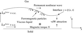
In this article we introduce a new physical effect in the evolution of thin liquid films endowed with rotational degrees of freedom (such liquids will henceforth be termed ‘structured’ following the terminology of Dahler & Scriven (Reference Dahler and Scriven1961)). A magnetic torque can drive the suspended particles in such a way that at the liquid–gas interface, their collective rotation (in a ‘conveyor-belt fashion’, see figure 1), described by the macroscopic particle angular velocity
 $\unicode[STIX]{x1D74E}$
(Shliomis Reference Shliomis1974, Reference Shliomis and Odenbach2002), manifests itself as an effective, non-uniform surface shear stress. The effect of such a stress is to provide a dominant horizontal component for the fluid velocity
 $\boldsymbol{u}$
, which causes an initial profile to steepen. Although a depression of the initial profile would deepen due to the attraction of the two interfaces, rupture is suppressed if the steepening wave catches up with the characteristic emanating from the bottom of the well, long before the liquid–gas interface reaches the solid substrate (Kirkinis & Davis Reference Kirkinis and Davis2015). As a direct consequence of the competition between the two effects (forcing and instability) a permanent nonlinear viscous–capillary wave is established.
In this article we consider an ultra-thin liquid film where the instability mechanism is due to intermolecular (van der Waals) forces that tend to attract the liquid–gas and liquid–solid interfaces leading to film rupture and substrate dewetting. The stabilizing effect of the interfacial particle collective rotation can also be employed in other systems such as a liquid film on the underside of a plate and a liquid film above a plate subject to interfacial temperature gradients. The former will experience a gravity-induced Rayleigh–Taylor instability (Oron, Davis & Bankoff Reference Oron, Davis and Bankoff1997) and the latter a thermocapillary instability whereby interfacial liquid is driven from depressions of the film thickness to peaks leading to thinning and possible rupture (Davis Reference Davis1987). A magnetic torque leading to interfacial particle collective rotation can then suppress both aforementioned instabilities.
A moving interface at
 $z=\unicode[STIX]{x1D709}(x,t)$
separates a gas from a viscous liquid lying on a solid substrate located at
 $z=0$
. Nanosize particles suspended in the carrier liquid rotate with a macroscopic angular velocity field
 $\unicode[STIX]{x1D74E}=\unicode[STIX]{x1D714}(x,z,t)\hat{\boldsymbol{y}}$
by responding to a magnetic torque density
 $N\hat{\boldsymbol{y}}=\boldsymbol{m}\times \boldsymbol{h}$
produced by an alternating magnetic field of frequency
 $\unicode[STIX]{x1D708}$
applied on the suspension of macroscopic magnetization
 $\boldsymbol{m}$
. The particle collective rotation near the liquid–gas interface induces a dominant horizontal liquid velocity component
 $u(x,z,t)\hat{\boldsymbol{x}}$
, that competes against the destabilizing van der Waals (vdW) forces that tend to deepen depressions of the liquid due to the attraction of the two interfaces. The competition of the two effects (forcing and instability) leads to the establishment of a permanent nonlinear viscous–capillary wave.

The present article is organized as follows. In § 2 we briefly review known results from the literature on the stabilization of thin liquid films in the absence of rotational degrees of freedom by pointing out the importance a surface shear has in the stabilization process. In § 3 we outline the theory of structured liquids which embodies the balance of internal angular momentum of suspended particles through their macroscopic angular velocity
 $\unicode[STIX]{x1D74E}$
. The conditions couple-stresses satisfy on a free surface of a structured liquid were derived in the theoretical analysis of Chaves & Rinaldi (Reference Chaves and Rinaldi2014). This point as well as other interfacial conditions are discussed in § 3.1. The reduction of the full Navier–Stokes and angular momentum equations in the geometry displayed in figure 1 is described in detail in § 4. Allowance is made for a body-force potential originating from intermolecular (van der Waals) attraction of the liquid–gas and liquid–solid interfaces. A body force of magnetic origin is not explicitly included in this discussion as its effects are subdominant to their magnetic torque counterpart (this point is discussed in appendix A). The reduction continues further in § 4.1 by resorting to the long wavelength approximation. This is possible to carry out because a thin liquid film possesses a geometrical disparity of spatial scales parallel and normal to the solid substrate. Thus, the very difficult free-boundary problem reduces to a tractable partial differential equation albeit fully nonlinear and including higher-order spatial derivatives. The flow, driven by the time-averaged torque (§ 4.2) leads to the generation of new nonlinear terms in the evolution equation for the liquid–gas profile. To understand their physical significance, the asymptotic limit of vanishing film thickness is considered which brings to prominence new convective terms of magnetic origin in the evolution equation (§ 5). In § 5.2 we calculate the critical torque required to bring about stabilization based on the corresponding mean-field analysis of Kirkinis & Davis (Reference Kirkinis and Davis2015). These estimates are in excellent agreement with the corresponding numerical simulations of the evolution equation. We conclude this article in § 6 with a discussion of how the present framework could, in principle, be employed to explain recent experimental results of interfacial rotation in a counter-rotating magnetic field in a ferrofluid (Chaves, Zahn & Rinaldi Reference Chaves, Zahn and Rinaldi2008) and the effect of the liquid’s rotational degrees of freedom on chiral particle swimming (Kirkinis, Andreev & Spivak Reference Kirkinis, Andreev and Spivak2012). For completeness, in appendix C, we include a brief discussion of the effects the interfacial slip (Dussan V Reference Dussan V1976) and surface shear ‘wind’ (Davis, Gratton & Davis Reference Davis, Gratton and Davis2010) have on the phenomenon developed in this article.
Although only suspensions of ferromagnetic particles driven by a magnetic field are considered in this article, analogous arguments can be applied to the case of particles endowed with an electric dipole moment and acted upon by an electric field.
2 Review of thin liquid film evolution in the absence of rotational degrees of freedom
Insight into the effect developed in the present article can be gained from known results on the long-scale evolution of a thin liquid film on a solid substrate at
 $Z=0$
and with the dimensionless liquid–gas interface profile located at
 $Z=\unicode[STIX]{x1D6EF}(X,T)$
(
 $\unicode[STIX]{x1D6EF}$
is the upper case counterpart of
 $\unicode[STIX]{x1D709}$
; the latter serves to denote the dimensional location of the liquid–gas interface at
 $z=\unicode[STIX]{x1D709}(x,t)$
in relation to the solid substrate at
 $z=0$
) of an unstructured liquid (Oron et al.
Reference Oron, Davis and Bankoff1997), i.e. of a classical Newtonian liquid
 $$\begin{eqnarray}\unicode[STIX]{x1D6EF}_{T}+\unicode[STIX]{x1D70F}\unicode[STIX]{x1D6EF}\unicode[STIX]{x1D6EF}_{X}+\left[A\frac{\unicode[STIX]{x1D6EF}_{X}}{\unicode[STIX]{x1D6EF}}+\frac{1}{3}\bar{C}^{-1}\unicode[STIX]{x1D6EF}^{3}\unicode[STIX]{x1D6EF}_{XXX}\right]_{X}=0,\end{eqnarray}$$
where an upper case Latin subscript here denotes differentiation with respect to the indicated dimensionless variable. The third term arises from consideration of van der Waals forces that tend to attract the liquid–gas and solid–liquid interfaces when the Hamaker constant
 $A$
is positive (Dzyaloshinskii et al.
Reference Dzyaloshinskii, Lifshitz and Pitaevskii1960, Reference Dzyaloshinskii, Lifshitz and Pitaevskii1961) which is the case considered in this article. The fourth term arises from the normal stress jump between the liquid and the gas phases separated by a common interface of curvature
 $K$
and surface tension
 $\unicode[STIX]{x1D6FE}$
and
 $\bar{C}$
is a scaled capillary number. The second term of (2.1) results from a constant shear
 $\unicode[STIX]{x1D70F}$
(whose origin may be wind blowing or temperature gradients)
 $$\begin{eqnarray}U_{Z}=\unicode[STIX]{x1D70F},\quad \text{at }Z=\unicode[STIX]{x1D6EF}(X,T),\end{eqnarray}$$
where
 $U$
is the dimensionless horizontal component of the fluid velocity. In the linear regime, a stability analysis (Oron et al.
Reference Oron, Davis and Bankoff1997; Davis Reference Davis, Batchelor, Moffatt and Worster2002) proceeds by perturbing the film profile at a constant elevation
 $\unicode[STIX]{x1D6EF}=1+\unicode[STIX]{x1D6FF}\text{e}^{\text{i}kX+\unicode[STIX]{x1D70E}T}$
, for perturbing parameter
 $\unicode[STIX]{x1D6FF}\ll 1$
, wavenumber
 $k$
and growth rate
 $\unicode[STIX]{x1D70E}$
, substituting into (2.1) and keeping only terms linear in
 $\unicode[STIX]{x1D6FF}$
. We thus obtain the standard growth rate relation (Kirkinis & Davis Reference Kirkinis and Davis2015)
 $$\begin{eqnarray}\unicode[STIX]{x1D70E}=Ak^{2}-(3\bar{C})^{-1}k^{4}.\end{eqnarray}$$
The shear-dependent part in (2.1) only contributes an imaginary term in (2.3) (not shown here) that is associated with wave propagation and does not affect stability in this linear analysis. Without repeating the details relating to (2.3) (Oron et al.
Reference Oron, Davis and Bankoff1997; Davis Reference Davis, Batchelor, Moffatt and Worster2002) we point out that when
 $A>0$
the wave numbers
 $0<k<(3A\bar{C})^{1/2}$
bring about instability since then the exponent
 $\unicode[STIX]{x1D70E}$
becomes positive. The physical consequence of this process is that depressions of the liquid–gas interface approach the solid substrate leading to film rupture and subsequently to substrate dewetting.
The shear
 $\unicode[STIX]{x1D70F}$
plays a vital role in any nonlinear analysis: in the absence of shear (
 $\unicode[STIX]{x1D70F}\equiv 0$
) the conclusions of the aforementioned linear analysis are in effect. For
 $\unicode[STIX]{x1D70F}\neq 0$
but small, the convective term in (2.1) breaks the reflection symmetry
 $x\rightarrow -x$
leading to the propagation of an interfacial wave which, however, cannot avert rupture (Kirkinis & Davis Reference Kirkinis and Davis2015). A sufficiently strong surface shear, on the other hand, that exceeds a critical value
 $\unicode[STIX]{x1D70F}_{c}$
, competes with the destabilizing effect of the attractive van der Waals forces. The competition of the two effects (forcing and instability) generates a permanent nonlinear viscous–capillary wave so that rupture and substrate dewetting are both averted.
Therefore, a surface shear, and the accompanying convective term (second term in (2.1)), plays a crucial role in stabilizing an unstable thin unstructured liquid film. In this article we will demonstrate that in a structured liquid, an external torque, through the mediation of the liquid’s rotational degrees of freedom, gives rise to the aforementioned collective interfacial particle rotation which leads to the appearance of new convective terms in the liquid–gas interface profile evolution equation that replace the second term in (2.1) and thus constitutes an alternative way of stabilizing an unstable thin liquid film.
3 Liquid film motion in the presence of rotational degrees of freedom
In a structured liquid (i.e. in a liquid with rotational degrees of freedom – a classical Newtonian liquid with small suspended particles that can respond to an external torque) the balance of linear and internal angular momentum can be expressed in the form (Dahler & Scriven Reference Dahler and Scriven1961; Condiff & Dahler Reference Condiff and Dahler1964)
 $$\begin{eqnarray}\unicode[STIX]{x1D70C}\text{D}u_{i}/\text{D}t=\unicode[STIX]{x2202}_{k}\unicode[STIX]{x1D70E}_{ik}\quad \text{and}\quad I\text{D}\unicode[STIX]{x1D714}_{i}/\text{D}t=\unicode[STIX]{x2202}_{k}\unicode[STIX]{x1D60A}_{ik}+N_{i}+\unicode[STIX]{x1D716}_{imk}\unicode[STIX]{x1D70E}_{km},\quad i,k,m=1,2,3,\end{eqnarray}$$
where
 $\text{D}/\text{D}t$
is the convective derivative,
 $\unicode[STIX]{x1D70C}$
is the fluid density,
 $I$
the volume density of particle moment of inertia,
 $u_{i}$
is the fluid velocity,
 $\unicode[STIX]{x1D714}_{i}$
the particle angular velocity and
 $N_{i}$
is the magnetic torque density. As noted by Dahler & Scriven (Reference Dahler and Scriven1961) the last term of the second equation in (3.1) represents the transformation of the moment of momentum
 $\unicode[STIX]{x1D716}_{ijk}x_{i}u_{j}$
into internal angular momentum only when the stress
 $\unicode[STIX]{x1D70E}_{ij}$
(not to be associated with the growth rate
 $\unicode[STIX]{x1D70E}$
of (2.3)) has an antisymmetric part. This part augments the standard Cauchy stress tensor and arises solely due to the inclusion of the nanostructure in the liquid. The resulting total stress
 $\unicode[STIX]{x1D748}$
is (Rinaldi Reference Rinaldi2002)
 $$\begin{eqnarray}\unicode[STIX]{x1D70E}_{ik}=-p\unicode[STIX]{x1D6FF}_{ik}+\unicode[STIX]{x1D702}\hat{\unicode[STIX]{x1D61D}}_{ik}+\unicode[STIX]{x1D701}\hat{\unicode[STIX]{x1D61E}}_{ik}+\hat{\unicode[STIX]{x1D61B}}_{ik},\end{eqnarray}$$
where
 $\hat{\unicode[STIX]{x1D61D}}_{ik}=\unicode[STIX]{x2202}_{k}u_{i}+\unicode[STIX]{x2202}_{i}u_{k}$
is the rate of shear strain,
 $\hat{\unicode[STIX]{x1D61E}}_{ik}=\unicode[STIX]{x2202}_{k}u_{i}-\unicode[STIX]{x2202}_{i}u_{k}-2\unicode[STIX]{x1D716}_{kil}\unicode[STIX]{x1D714}_{l}$
is a ‘spin’ tensor measuring the imbalance between liquid and particle angular velocity,
 $\hat{\unicode[STIX]{x1D61B}}_{ik}=(h_{i}b_{k}-(1/2)h_{j}^{2}\unicode[STIX]{x1D6FF}_{ik})/4\unicode[STIX]{x03C0}$
is the Maxwell stress tensor and
 $\boldsymbol{h}$
and
 $\boldsymbol{b}$
denote the macroscopic magnetic field and induction, respectively. The liquid is considered incompressible
 $\unicode[STIX]{x2202}_{i}u_{i}=0$
,
 $p$
is the hydrostatic pressure and
 $\unicode[STIX]{x1D702}$
is the liquid viscosity. The phenomenological coefficient
 $\unicode[STIX]{x1D701}$
multiplying
 $\hat{\unicode[STIX]{x1D652}}$
in (3.2) is termed the vortex viscosity in the literature (Condiff & Dahler Reference Condiff and Dahler1964; Rinaldi Reference Rinaldi2002).
 $\unicode[STIX]{x1D716}_{ijk}$
is the alternating pseudo-tensor and we employed the Einstein summation convention on repeated indices.
 $\hat{\unicode[STIX]{x1D652}}$
has
 $\text{curl}\boldsymbol{u}-2\unicode[STIX]{x1D74E}$
as its axial vector. When this vector vanishes identically in the body of a slowly flowing viscous liquid in the absence of externally applied torques and non-conservative forces, the balance of internal angular momentum in (3.1) is automatically satisfied and the balance of linear momentum in (3.1) reduces to the standard Navier–Stokes equations satisfied by the velocity field of an unstructured liquid (Condiff & Dahler Reference Condiff and Dahler1964). Since in this case the structured liquid behaves as a standard Newtonian liquid, it will suffer the same instabilities and in particular rupture by van der Waals forces.
Diffusion of internal angular momentum takes place due to the couple stresses
 $\unicode[STIX]{x1D63E}$
 $$\begin{eqnarray}\unicode[STIX]{x1D60A}_{ik}=\unicode[STIX]{x1D702}^{\prime }\left(\unicode[STIX]{x2202}_{k}\unicode[STIX]{x1D714}_{i}+\unicode[STIX]{x2202}_{i}\unicode[STIX]{x1D714}_{k}\right)+\unicode[STIX]{x1D701}^{\prime }\unicode[STIX]{x2202}_{j}\unicode[STIX]{x1D714}_{j}\unicode[STIX]{x1D6FF}_{ik},\end{eqnarray}$$
the suspended particles experience in their rotational motion. Here
 $\unicode[STIX]{x1D702}^{\prime }$
and
 $\unicode[STIX]{x1D701}^{\prime }$
are the shear and bulk coefficients of spin viscosity (Condiff & Dahler Reference Condiff and Dahler1964). Therefore,
 $\unicode[STIX]{x2202}_{j}\unicode[STIX]{x1D60A}_{ij}$
in (3.1) is the rate of arrival of internal angular momentum by way of diffusion. Maxwell’s equations are
 $\unicode[STIX]{x1D735}\times \boldsymbol{h}=0$
and
 $\unicode[STIX]{x1D735}\boldsymbol{\cdot }\boldsymbol{b}=0$
, where
 $\boldsymbol{b}=\boldsymbol{h}+4\unicode[STIX]{x03C0}\boldsymbol{m}$
. Since the torque density
 $\boldsymbol{N}=\boldsymbol{m}\times \boldsymbol{h}$
depends on the macroscopic magnetization field
 $\boldsymbol{m}$
of suspended particles, one more constitutive equation describing the evolution of this field has to be imposed in order to provide closure (Rinaldi Reference Rinaldi2002). This is
 $$\begin{eqnarray}\text{D}m_{i}/\text{D}t=\unicode[STIX]{x1D716}_{ijk}\unicode[STIX]{x1D714}_{j}m_{k}-(m_{i}-\unicode[STIX]{x1D712}h_{i})/t_{s}\quad i=1,2,3.\end{eqnarray}$$
Here
 $t_{s}$
is a relaxation time and
 $\unicode[STIX]{x1D712}$
is the effective magnetic susceptibility. We consider this to be a constant which is a common assumption for weak fields (Zahn & Greer Reference Zahn and Greer1995).
3.1 Boundary conditions
At a liquid–gas interface with mean curvature
 $K$
and constant surface tension
 $\unicode[STIX]{x1D6FE}$
, continuity of traction implies
 $-[[\unicode[STIX]{x1D748}\boldsymbol{n}]]+2K\unicode[STIX]{x1D6FE}\boldsymbol{n}=0$
(Oron et al.
Reference Oron, Davis and Bankoff1997), where
 $\boldsymbol{n}$
and
 $\boldsymbol{t}$
are the normal and tangent unit vectors at this interface respectively and the symbol
 $[[\cdot ]]$
denotes the jump of the field across an interface. Thus, for the shear and normal stresses we have
 $$\begin{eqnarray}[[\boldsymbol{t}\unicode[STIX]{x1D748}\boldsymbol{n}]]=0,\quad \text{and}\quad [[\boldsymbol{n}\unicode[STIX]{x1D748}\boldsymbol{n}]]=2K\unicode[STIX]{x1D6FE},\end{eqnarray}$$
on the liquid-gas interface, while the couple-stress tensor
 $\unicode[STIX]{x1D63E}$
satisfies (Chaves & Rinaldi Reference Chaves and Rinaldi2014)
 $$\begin{eqnarray}[[\unicode[STIX]{x1D63E}\boldsymbol{n}]]=0.\end{eqnarray}$$
At the liquid–solid interface the no-slip and no-penetration conditions read
 $$\begin{eqnarray}\boldsymbol{u}\boldsymbol{\cdot }\boldsymbol{n}=0,\quad \boldsymbol{u}\boldsymbol{\cdot }\boldsymbol{t}=0.\end{eqnarray}$$
When required, the former can be relaxed and be replaced by a slip model as is usual in thin liquid film and droplet studies (Oron et al. Reference Oron, Davis and Bankoff1997; Kirkinis & Davis Reference Kirkinis and Davis2013, Reference Kirkinis and Davis2014), see appendix C. Finally we consider the particle angular velocity to vanish at the liquid–solid interface
 $$\begin{eqnarray}\unicode[STIX]{x1D74E}=0.\end{eqnarray}$$
Although this is a simplifying condition used in studies of magnetic liquids (Rinaldi & Zahn Reference Rinaldi and Zahn2002; Chaves et al. Reference Chaves, Zahn and Rinaldi2008), in the present article it becomes a necessity: other forms used in the literature are discarded here since they lead to unphysical results such as surface tension acting in a destabilizing fashion.
At the liquid–gas interface the induction and magnetic field components are continuous
 $$\begin{eqnarray}[[\boldsymbol{b}\boldsymbol{\cdot }\boldsymbol{n}]]=0\quad \text{and}\quad [[\boldsymbol{h}\boldsymbol{\cdot }\boldsymbol{t}]]=0.\end{eqnarray}$$
4 Reduction of the equations of motion
In the geometry displayed in figure 1 and in dimensional units, the liquid–gas interface lies at
 $z=\unicode[STIX]{x1D709}(x,t)$
and the solid–liquid interface at
 $z=0$
. The fluid velocity
 $\boldsymbol{u}$
, macroscopic particle angular velocity
 $\unicode[STIX]{x1D74E}$
and magnetization
 $\boldsymbol{m}$
obtain the component forms
 $(u(x,z,t),0,w(x,z,t))$
,
 $(0,\unicode[STIX]{x1D714}(x,z,t),0)$
and
 $(m_{1}(x,z,t),0,m_{3}(x,z,t))$
, respectively. The magnetic field
 $h_{1}={\hat{h}}_{1}\text{e}^{2\unicode[STIX]{x03C0}\text{i}\unicode[STIX]{x1D708}t}+\text{c.c.}$
and induction field
 $b_{3}=\hat{b}_{3}\text{e}^{2\unicode[STIX]{x03C0}\text{i}\unicode[STIX]{x1D708}t}+\text{c.c.}$
as displayed in figure 1, where c.c. stands for the complex conjugate, are considered to have constant amplitudes for simplicity and vary harmonically with frequency
 $\unicode[STIX]{x1D708}$
. The stress tensor (3.2) has the following non-vanishing components
 $\unicode[STIX]{x1D70E}_{11}=-p+2\unicode[STIX]{x1D702}u_{x}$
,
 $\unicode[STIX]{x1D70E}_{33}=-p+2\unicode[STIX]{x1D702}w_{z}$
,
 $\unicode[STIX]{x1D70E}_{13}=(\unicode[STIX]{x1D702}+\unicode[STIX]{x1D701})u_{z}+(\unicode[STIX]{x1D702}-\unicode[STIX]{x1D701})w_{x}-2\unicode[STIX]{x1D701}\unicode[STIX]{x1D714}$
,
 $\unicode[STIX]{x1D70E}_{31}=(\unicode[STIX]{x1D702}-\unicode[STIX]{x1D701})u_{z}+(\unicode[STIX]{x1D702}+\unicode[STIX]{x1D701})w_{x}+2\unicode[STIX]{x1D701}\unicode[STIX]{x1D714}$
where a lower case Latin subscript denotes differentiation with respect to the corresponding dimensional variable. For clarity and brevity we did not manifestly include the Maxwell stress tensor components in these expressions because they only give rise to a body force whose effects are subdominant to those of the torque studied in the present article (assuming weak fields and slow rotations, see the discussion in appendix A). The couple-stress tensor
 $\unicode[STIX]{x1D63E}$
has the following non-zero components
 $\unicode[STIX]{x1D60A}_{12}=\unicode[STIX]{x1D60A}_{21}=\unicode[STIX]{x1D714}_{x}$
and
 $\unicode[STIX]{x1D60A}_{23}=\unicode[STIX]{x1D60A}_{32}=\unicode[STIX]{x1D714}_{z}$
(
 $\unicode[STIX]{x2202}_{j}\unicode[STIX]{x1D714}_{j}=0$
is here satisfied identically). Then, the governing equations (2.1) reduce to
 $$\begin{eqnarray}\displaystyle & \displaystyle \unicode[STIX]{x1D70C}[u_{t}+uu_{x}+wu_{z}]=-p_{x}-2\unicode[STIX]{x1D701}\unicode[STIX]{x1D714}_{z}+(\unicode[STIX]{x1D701}+\unicode[STIX]{x1D702})(u_{xx}+u_{zz})-\unicode[STIX]{x1D719}_{x}, & \displaystyle\end{eqnarray}$$
 $$\begin{eqnarray}\displaystyle & \displaystyle \unicode[STIX]{x1D70C}[w_{t}+uw_{x}+ww_{z}]=-p_{z}+2\unicode[STIX]{x1D701}\unicode[STIX]{x1D714}_{x}+(\unicode[STIX]{x1D701}+\unicode[STIX]{x1D702})(w_{xx}+w_{zz})-\unicode[STIX]{x1D719}_{z}, & \displaystyle\end{eqnarray}$$
 $$\begin{eqnarray}\displaystyle & \displaystyle I[\unicode[STIX]{x1D714}_{t}+u\unicode[STIX]{x1D714}_{x}+w\unicode[STIX]{x1D714}_{z}]=2\unicode[STIX]{x1D701}(u_{z}-w_{x}-2\unicode[STIX]{x1D714})+\unicode[STIX]{x1D702}^{\prime }(\unicode[STIX]{x1D714}_{xx}+\unicode[STIX]{x1D714}_{zz})+N, & \displaystyle\end{eqnarray}$$
where
 $N$
is an applied torque and the potential
 $\unicode[STIX]{x1D719}$
is associated with attractive van der Waals forces (Dzyaloshinskii et al.
Reference Dzyaloshinskii, Lifshitz and Pitaevskii1960) which tend to bring the liquid–gas and liquid–solid interfaces together. It is given by
 $\unicode[STIX]{x1D719}=\unicode[STIX]{x1D719}_{r}+A^{\prime }\unicode[STIX]{x1D709}^{-3}/6\unicode[STIX]{x03C0}$
where
 $\unicode[STIX]{x1D719}_{r}$
is a reference value and
 $A^{\prime }>0$
(negative disjoining pressure) is the dimensional Hamaker constant. The boundary conditions (3.7) and (3.8) become
 $$\begin{eqnarray}u=0,\quad w=0\quad \text{and}\quad \unicode[STIX]{x1D714}=0,\quad \text{at }z=0,\end{eqnarray}$$
respectively. The tangent and normal vectors to the interface are
 $\boldsymbol{t}=(1,\unicode[STIX]{x1D709}_{x})/\sqrt{1+\unicode[STIX]{x1D709}_{x}^{2}}$
and
 $\boldsymbol{n}=(-\unicode[STIX]{x1D709}_{x},1)/\sqrt{1+\unicode[STIX]{x1D709}_{x}^{2}}$
respectively. Thus, at the liquid–gas interface
 $z=\unicode[STIX]{x1D709}(x,t)$
the boundary conditions (3.5) read
 $$\begin{eqnarray}\unicode[STIX]{x1D70E}_{13}-\unicode[STIX]{x1D709}_{x}^{2}\unicode[STIX]{x1D70E}_{31}+\unicode[STIX]{x1D709}_{x}(\unicode[STIX]{x1D70E}_{33}-\unicode[STIX]{x1D70E}_{11})=0\quad \text{and}\quad \frac{1}{1+\unicode[STIX]{x1D709}_{x}^{2}}\left[\unicode[STIX]{x1D70E}_{33}+\unicode[STIX]{x1D709}_{x}^{2}\unicode[STIX]{x1D70E}_{11}-\unicode[STIX]{x1D709}_{x}(\unicode[STIX]{x1D70E}_{13}+\unicode[STIX]{x1D70E}_{31})\right]=2K\unicode[STIX]{x1D6FE},\end{eqnarray}$$
where
 $2K=\unicode[STIX]{x1D709}_{xx}/\sqrt{1+\unicode[STIX]{x1D709}_{x}^{2}}$
. Equation (3.6) becomes
 $$\begin{eqnarray}\unicode[STIX]{x1D714}_{z}-\unicode[STIX]{x1D709}_{x}\unicode[STIX]{x1D714}_{x}=0.\end{eqnarray}$$
To the above one may add the kinematic condition
 $$\begin{eqnarray}w=\unicode[STIX]{x1D709}_{t}+u\unicode[STIX]{x1D709}_{x}\end{eqnarray}$$
at the liquid–gas interface
 $z=\unicode[STIX]{x1D709}(x,t)$
which constitutes the starting point in deriving the sought after evolution equation. The conditions (3.9) are used to simplify the components of the Maxwell stress tensor.
4.1 Lubrication approximation
In this approximation the Navier–Stokes and internal angular momentum equations are scaled with respect to a long wavelength
 $\unicode[STIX]{x1D706}$
which is a natural consequence of the longitudinal and vertical disparity of scales embodied in a thin liquid film. This introduces slow longitudinal and slow temporal variables
 $$\begin{eqnarray}X=\frac{2\unicode[STIX]{x03C0}x}{\unicode[STIX]{x1D706}}=\unicode[STIX]{x1D716}\frac{x}{\unicode[STIX]{x1D709}_{0}},\quad Z=\frac{z}{\unicode[STIX]{x1D709}_{0}},\quad \text{and}\quad T=\frac{2\unicode[STIX]{x03C0}U_{0}}{\unicode[STIX]{x1D706}}t,\quad \text{for }\unicode[STIX]{x1D716}=\frac{2\unicode[STIX]{x03C0}\unicode[STIX]{x1D709}_{0}}{\unicode[STIX]{x1D706}},\end{eqnarray}$$
where
 $\unicode[STIX]{x1D709}_{0}$
and
 $U_{0}$
are characteristic scales for the liquid film thickness and longitudinal velocity respectively and the partial derivatives
 $\unicode[STIX]{x2202}/\unicode[STIX]{x2202}X$
and
 $\unicode[STIX]{x2202}/\unicode[STIX]{x2202}Z$
are now quantities of unit order (Davis Reference Davis, Batchelor, Moffatt and Worster2002). The velocity, particle angular velocity, pressure and liquid–gas interface location become respectively
 $$\begin{eqnarray}U=\frac{u}{U_{0}},\quad W=\frac{\unicode[STIX]{x1D706}}{2\unicode[STIX]{x03C0}\unicode[STIX]{x1D709}_{0}}\frac{w}{U_{0}}=\frac{1}{\unicode[STIX]{x1D716}}\frac{w}{U_{0}},\quad \unicode[STIX]{x1D6FA}=\frac{\unicode[STIX]{x1D714}}{\unicode[STIX]{x1D6FA}_{0}},\quad P=\frac{2\unicode[STIX]{x03C0}\unicode[STIX]{x1D709}_{0}}{\unicode[STIX]{x1D706}}\frac{\unicode[STIX]{x1D709}_{0}p}{(\unicode[STIX]{x1D702}+\unicode[STIX]{x1D701})U_{0}},\quad \unicode[STIX]{x1D6EF}=\frac{\unicode[STIX]{x1D709}}{\unicode[STIX]{x1D709}_{0}},\end{eqnarray}$$
where
 $\unicode[STIX]{x1D6FA}_{0}$
is a characteristic scale for the particle angular velocity
 $\unicode[STIX]{x1D714}$
.
We define the dimensionless Reynolds numbers, Hamaker constant and scaled capillary number
 $$\begin{eqnarray}Re=\frac{U_{0}\unicode[STIX]{x1D709}_{0}\unicode[STIX]{x1D70C}}{\unicode[STIX]{x1D702}+\unicode[STIX]{x1D701}},\quad Re^{\prime }=\frac{IU_{0}\unicode[STIX]{x1D709}_{0}}{\unicode[STIX]{x1D702}^{\prime }},\quad A=\frac{A^{\prime }\unicode[STIX]{x1D716}}{6\unicode[STIX]{x03C0}(\unicode[STIX]{x1D702}+\unicode[STIX]{x1D701})\unicode[STIX]{x1D709}_{0}^{2}U_{0}},\quad \bar{C}=\unicode[STIX]{x1D716}^{-3}\frac{U_{0}(\unicode[STIX]{x1D702}+\unicode[STIX]{x1D701})}{\unicode[STIX]{x1D6FE}}\end{eqnarray}$$
(for simplicity we will set
 $U_{0}=\unicode[STIX]{x1D709}_{0}\unicode[STIX]{x1D6FA}_{0}$
) and dimensionless potential, torque, magnetic field, induction and magnetization
 $$\begin{eqnarray}\unicode[STIX]{x1D6F7}=\frac{\unicode[STIX]{x1D716}\unicode[STIX]{x1D709}_{0}\unicode[STIX]{x1D719}}{(\unicode[STIX]{x1D702}+\unicode[STIX]{x1D701})U_{0}},\quad {\mathcal{N}}=\frac{N\unicode[STIX]{x1D709}_{0}^{2}}{\unicode[STIX]{x1D702}^{\prime }\unicode[STIX]{x1D6FA}_{0}},\quad H_{i}=\frac{h_{i}}{H_{0}},\quad B_{i}=\frac{b_{i}}{H_{0}},\quad M_{i}=\frac{m_{i}}{\unicode[STIX]{x1D712}H_{0}},\end{eqnarray}$$
where
 $H_{0}$
is a characteristic value of the magnetic field
 $H$
. Finally we define the dimensionless driving frequency, relaxation time and subsidiary dimensionless parameters
 $\unicode[STIX]{x1D6FC},\unicode[STIX]{x1D6FD}$
and
 $\unicode[STIX]{x1D705}$
 $$\begin{eqnarray}\bar{\unicode[STIX]{x1D708}}=\unicode[STIX]{x1D708}\frac{\unicode[STIX]{x1D709}_{0}}{U_{0}},\quad \bar{\unicode[STIX]{x1D70F}}=t_{s}\frac{U_{0}}{\unicode[STIX]{x1D709}_{0}},\quad \unicode[STIX]{x1D6FC}=\frac{\unicode[STIX]{x1D701}}{\unicode[STIX]{x1D702}+\unicode[STIX]{x1D701}},\quad \unicode[STIX]{x1D6FD}=2\frac{\unicode[STIX]{x1D701}\unicode[STIX]{x1D709}_{0}^{2}}{\unicode[STIX]{x1D702}^{\prime }},\quad \unicode[STIX]{x1D705}^{2}\equiv 2\unicode[STIX]{x1D6FD}(1-\unicode[STIX]{x1D6FC})=\frac{4\unicode[STIX]{x1D702}\unicode[STIX]{x1D701}\unicode[STIX]{x1D709}_{0}^{2}}{\unicode[STIX]{x1D702}^{\prime }(\unicode[STIX]{x1D702}+\unicode[STIX]{x1D701})}.\end{eqnarray}$$
With the above notation, equations (4.1)–(4.3) obtain the following dimensionless form
 $$\begin{eqnarray}\displaystyle & \displaystyle \unicode[STIX]{x1D716}\mathit{Re}\left[U_{T}+UU_{X}+WU_{Z}\right]=-P_{X}-2\unicode[STIX]{x1D6FC}\unicode[STIX]{x1D6FA}_{Z}+(\unicode[STIX]{x1D716}^{2}U_{XX}+U_{ZZ})-\unicode[STIX]{x1D6F7}_{X}, & \displaystyle\end{eqnarray}$$
 $$\begin{eqnarray}\displaystyle & \displaystyle \unicode[STIX]{x1D716}^{2}\mathit{Re}\left[W_{T}+UW_{X}+WW_{Z}\right]=-\frac{1}{\unicode[STIX]{x1D716}}P_{Z}+2\unicode[STIX]{x1D716}\unicode[STIX]{x1D6FC}\unicode[STIX]{x1D6FA}_{X}+\unicode[STIX]{x1D716}(\unicode[STIX]{x1D716}^{2}W_{XX}+W_{ZZ})-\frac{1}{\unicode[STIX]{x1D716}}\unicode[STIX]{x1D6F7}_{Z}, & \displaystyle\end{eqnarray}$$
 $$\begin{eqnarray}\displaystyle & \displaystyle \unicode[STIX]{x1D716}\mathit{Re}^{\prime }\left[\unicode[STIX]{x1D6FA}_{T}+U\unicode[STIX]{x1D6FA}_{X}+W\unicode[STIX]{x1D6FA}_{Z}\right]=\unicode[STIX]{x1D6FD}(U_{Z}-\unicode[STIX]{x1D716}^{2}W_{X}-2\unicode[STIX]{x1D6FA})+\unicode[STIX]{x1D716}^{2}\unicode[STIX]{x1D6FA}_{XX}+\unicode[STIX]{x1D6FA}_{ZZ}+{\mathcal{N}}. & \displaystyle\end{eqnarray}$$
The boundary conditions (4.4), (4.5), (4.6), become respectively
 $$\begin{eqnarray}U=0,\quad W=0,\quad \unicode[STIX]{x1D6FA}=0,\quad \text{at }Z=0,\end{eqnarray}$$
and
 $$\begin{eqnarray}U_{Z}-2\unicode[STIX]{x1D6FC}\unicode[STIX]{x1D6FA}+O(\unicode[STIX]{x1D716})=0,\quad -P=\bar{C}^{-1}\unicode[STIX]{x1D6EF}_{XX}+O(\unicode[STIX]{x1D716}),\quad \unicode[STIX]{x1D6FA}_{Z}+O(\unicode[STIX]{x1D716})=0,\quad \text{at }Z=\unicode[STIX]{x1D6EF}(X,T).\end{eqnarray}$$
The kinematic condition (4.7) becomes
 $W=\unicode[STIX]{x1D6EF}_{T}+U\unicode[STIX]{x1D6EF}_{X}$
and leads to the following evolution equation for the profile
 $\unicode[STIX]{x1D6EF}$
:
 $$\begin{eqnarray}\unicode[STIX]{x1D6EF}_{T}+\left[\int _{0}^{\unicode[STIX]{x1D6EF}}U\,\text{d}Z\right]_{X}=0.\end{eqnarray}$$
This is obtained in the standard way (Oron et al.
Reference Oron, Davis and Bankoff1997) by integrating the incompressibility condition
 $U_{X}+W_{Z}=0$
from
 $Z=0$
to
 $Z=\unicode[STIX]{x1D6EF}(X,T)$
, using (4.16b
) and integration by parts.
We proceed by expanding all fields in a regular perturbation expansion with respect to the small parameter
 $\unicode[STIX]{x1D716}$
:
 $(U,W,P,\unicode[STIX]{x1D6FA})=(U^{0},W^{0},P^{0},\unicode[STIX]{x1D6FA}^{0})+\unicode[STIX]{x1D716}(U^{1},W^{1},P^{1},\unicode[STIX]{x1D6FA}^{1})+O(\unicode[STIX]{x1D716}^{2})$
. To leading order (which corresponds to the lubrication approximation) and dropping superscripts denoting order in
 $\unicode[STIX]{x1D716}$
, the scaled equations (4.13)–(4.15) and the magnetization equation and Maxwell’s equations (the derivation of the latter is discussed in appendix B) simplify to
 $$\begin{eqnarray}-P_{X}-2\unicode[STIX]{x1D6FC}\unicode[STIX]{x1D6FA}_{Z}+U_{ZZ}=0,\quad -P_{Z}-\unicode[STIX]{x1D6F7}_{Z}=0,\quad \unicode[STIX]{x1D6FD}(U_{Z}-2\unicode[STIX]{x1D6FA})+\unicode[STIX]{x1D6FA}_{ZZ}+{\mathcal{N}}=0,\end{eqnarray}$$
 $$\begin{eqnarray}(2\unicode[STIX]{x03C0}\text{i}\bar{\unicode[STIX]{x1D708}}\bar{\unicode[STIX]{x1D70F}}+1)\hat{M}_{1}-\bar{\unicode[STIX]{x1D70F}}\unicode[STIX]{x1D6FA}\hat{M}_{3}={\hat{H}}_{1},\quad \bar{\unicode[STIX]{x1D70F}}\unicode[STIX]{x1D6FA}\hat{M}_{1}+(2\unicode[STIX]{x03C0}\text{i}\bar{\unicode[STIX]{x1D708}}\bar{\unicode[STIX]{x1D70F}}+1+4\unicode[STIX]{x03C0}\unicode[STIX]{x1D712})\hat{M}_{3}=\hat{B}_{3},\end{eqnarray}$$
 $$\begin{eqnarray}H_{1,Z}=0,\quad B_{3,Z}=0,\end{eqnarray}$$
where the driving frequency
 $\bar{\unicode[STIX]{x1D708}}$
and relaxation time
 $\bar{\unicode[STIX]{x1D70F}}$
were defined in (4.12) (also see appendix B) and an upper case Latin subscript preceded by a comma denotes differentiation with respect to the corresponding dimensionless variable. The (complex) amplitude of a field is superposed by a hat (see appendix B). The boundary conditions at the liquid–gas interface read
 $$\begin{eqnarray}U_{Z}-2\unicode[STIX]{x1D6FC}\unicode[STIX]{x1D6FA}=0,\quad -P=\bar{C}^{-1}\unicode[STIX]{x1D6EF}_{XX},\quad \unicode[STIX]{x1D6FA}_{Z}=0,\quad \text{at }Z=\unicode[STIX]{x1D6EF}(X,T),\end{eqnarray}$$
and the boundary conditions at the liquid–solid interface remain the same as (4.16) with the understanding that they now refer to the leading-order approximation.
Integration of the second of (4.19) and application of the normal stress boundary condition (second of (4.22)) leads to
 $\bar{P}(X,T)\equiv P+\unicode[STIX]{x1D6F7}=\unicode[STIX]{x1D6F7}|_{Z=\unicode[STIX]{x1D6EF}}-\bar{C}^{-1}\unicode[STIX]{x1D6EF}_{XX}$
.
4.2 Time-averaged torque
The dimensional time-averaged torque (Zahn & Greer Reference Zahn and Greer1995, (30)) is
 $$\begin{eqnarray}\langle N\rangle =\text{Re}\left\{m_{3}h_{1}^{\ast }-m_{1}b_{3}^{\ast }+4\unicode[STIX]{x03C0}m_{3}m_{1}^{\ast }\right\}/2,\end{eqnarray}$$
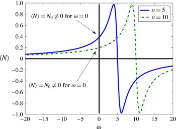
displayed in figure 3,
 $\text{Re}$
denotes the real part of a complex number and the symbol
 $\langle \cdot \rangle$
denotes time averaging over the period of oscillation. For small values of angular velocity
 $\unicode[STIX]{x1D714}$
the torque can be expanded as
 $\langle N\rangle =N_{0}+N_{1}\unicode[STIX]{x1D714}+O(\unicode[STIX]{x1D714}^{2})$
. The constants
 $N_{i},\hspace{2.22198pt}i=0,1,\ldots$
depend on the field frequency
 $\unicode[STIX]{x1D708}$
and amplitude, relaxation time
 $t_{s}$
and magnetic susceptibility
 $\unicode[STIX]{x1D712}$
. Figure 3 demonstrates that a constant torque
 $N_{0}$
is present when the fields differ in phase by
 $\unicode[STIX]{x03C0}/2$
: because there is a window of frequencies
 $\unicode[STIX]{x1D708}$
where
 $N_{0}$
can become very large, we will consider only the case of constant torque and slow rotation from now on (Zahn & Greer Reference Zahn and Greer1995, (35)). Then, equation (4.19) yield closed form expressions for the fields
 $U,W$
and
 $\unicode[STIX]{x1D6FA}$
and the flux function in (4.18) becomes
 $$\begin{eqnarray}\displaystyle \int _{0}^{\unicode[STIX]{x1D6EF}}U\,\text{d}Z & = & \displaystyle \frac{\unicode[STIX]{x1D6FC}}{\unicode[STIX]{x1D705}^{2}(1-\unicode[STIX]{x1D6FC})}\left\{\frac{\bar{P}_{X}}{\unicode[STIX]{x1D705}}\left[\frac{\unicode[STIX]{x1D705}\unicode[STIX]{x1D6EF}-\sinh \unicode[STIX]{x1D705}\unicode[STIX]{x1D6EF}+\unicode[STIX]{x1D705}\unicode[STIX]{x1D6EF}(\unicode[STIX]{x1D705}\unicode[STIX]{x1D6EF}\sinh (\unicode[STIX]{x1D705}\unicode[STIX]{x1D6EF})+1)}{\cosh \unicode[STIX]{x1D705}\unicode[STIX]{x1D6EF}}\right.\right.\nonumber\\ \displaystyle & & \displaystyle \left.\left.-\,\frac{1}{3\unicode[STIX]{x1D6FC}}\unicode[STIX]{x1D705}^{3}\unicode[STIX]{x1D6EF}^{3}-\unicode[STIX]{x1D705}\unicode[STIX]{x1D6EF}\right]+\frac{{\mathcal{N}}}{\unicode[STIX]{x1D6FD}}\left[\frac{1}{2}\unicode[STIX]{x1D705}^{2}\unicode[STIX]{x1D6EF}^{2}+1-\frac{1+\unicode[STIX]{x1D705}\unicode[STIX]{x1D6EF}\sinh \unicode[STIX]{x1D705}\unicode[STIX]{x1D6EF}}{\cosh \unicode[STIX]{x1D705}\unicode[STIX]{x1D6EF}}\right]\right\},\qquad\end{eqnarray}$$
where the parameters
 $\unicode[STIX]{x1D6FC}$
,
 $\unicode[STIX]{x1D6FD}$
and
 $\unicode[STIX]{x1D705}$
were defined in (4.12). This equation should be contrasted to the flux function
 $\int _{0}^{\unicode[STIX]{x1D6EF}}U\,\text{d}Z=-(1/3)\bar{P}_{X}\unicode[STIX]{x1D6EF}^{3}$
obtained in the absence of the rotational degrees of freedom (Oron et al.
Reference Oron, Davis and Bankoff1997; Davis Reference Davis, Batchelor, Moffatt and Worster2002).
4.3 Linear stability analysis and asymptotic limit
This analysis proceeds as in § 2. The dispersion relation is identical to (2.3) with the exception of renormalized values for
 $A$
and
 $\bar{C}$
arising from the inclusion of microstructure in the model. This analysis again shows that, when
 $A>0$
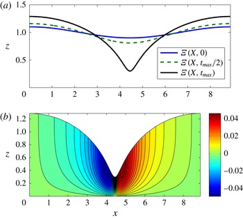
the film ruptures (cf. figure 2
a).
To obtain the physical meaning embodied in the flux function (4.24) we seek its asymptotic limit as
 $\unicode[STIX]{x1D6EF}\rightarrow 0$
 $$\begin{eqnarray}\int _{0}^{\unicode[STIX]{x1D6EF}}U\,\text{d}Z=-\frac{1}{3}\bar{P}_{X}\unicode[STIX]{x1D6EF}^{3}+\frac{\unicode[STIX]{x1D6FC}}{4}{\mathcal{N}}\unicode[STIX]{x1D6EF}^{4}-\frac{\unicode[STIX]{x1D6FC}\unicode[STIX]{x1D6FD}}{10}\bar{P}_{X}\unicode[STIX]{x1D6EF}^{5}-\frac{7\unicode[STIX]{x1D6FC}\unicode[STIX]{x1D6FD}(1-\unicode[STIX]{x1D6FC})}{36}{\mathcal{N}}\unicode[STIX]{x1D6EF}^{6}+O(\unicode[STIX]{x1D6EF}^{7}).\end{eqnarray}$$
The first term on the right-hand side of (4.25) is of the standard form encountered in the lubrication theories of thin liquid films but the higher-order terms are new.
Transition to rupture of a structured liquid film (i.e. a liquid film with suspended magnetic particles) under the influence of attractive van der Waals intermolecular forces. (a) Snapshots of the dimensionless liquid–gas interface
 $Z=\unicode[STIX]{x1D6EF}(X,T)$
. (b) Snapshot of the spatial distribution of the dimensionless particle angular velocity
 $\unicode[STIX]{x1D6FA}(X,Z,T)$
at
 $T=t_{max}$
. The motion of the particles is here weakly driven by the pressure gradient
 $\unicode[STIX]{x2202}_{X}P$
.

Plot of the time-averaged torque (4.23) versus particle angular velocity
 $\unicode[STIX]{x1D714}$
. For fields differing in phase by
 $\unicode[STIX]{x03C0}/2$
the torque obtains a non-zero value even when the angular velocity vanishes.

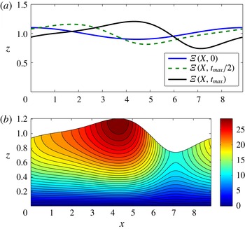
(a) Snapshots of the liquid–gas interface
 $Z=\unicode[STIX]{x1D6EF}(X,T)$
. The torque-induced collective rotation of the particles at the free surface competes with the van-der-Waals-driven instability establishing a permanent interfacial finite-amplitude wave. (b) Snapshot of the spatial distribution of the dimensionless particle angular velocity
 $\unicode[STIX]{x1D6FA}(X,Z,T)$
at
 $T=t_{max}$
. Surface particles rotate collectively in a ‘conveyor-belt’ fashion.

5 Magnetic torque-induced stabilization
The physical effect we introduce in this article is predominantly dependent on the form the shear stress condition
 $[[\boldsymbol{t}\unicode[STIX]{x1D748}\boldsymbol{n}]]=0$
acquires on the liquid–gas interface i.e. the first of (4.22) which, in dimensional form, reads
 $u_{z}=2\unicode[STIX]{x1D701}(\unicode[STIX]{x1D702}+\unicode[STIX]{x1D701})^{-1}\unicode[STIX]{x1D714}$
on
 $z=\unicode[STIX]{x1D709}(x,t)$
. The magnetic torque
 $\langle {\mathcal{N}}\rangle$
leads to a collective rotation at the free surface in a ‘conveyor-belt’ fashion due to the relatively uninhibited particle rotation there (cf. figure 4
b). Substituting (4.25) into (4.18) and retaining only leading-order terms in
 $\unicode[STIX]{x1D6EF}$
leads to the following evolution equation for the liquid–gas interface
 $$\begin{eqnarray}\unicode[STIX]{x1D6EF}_{T}+A\left(\frac{\unicode[STIX]{x1D6EF}_{X}}{\unicode[STIX]{x1D6EF}}\right)_{X}+\frac{1}{3}\bar{C}^{-1}\left(\unicode[STIX]{x1D6EF}^{3}\unicode[STIX]{x1D6EF}_{XXX}\right)_{X}+\unicode[STIX]{x1D6FC}{\mathcal{N}}\unicode[STIX]{x1D6EF}^{3}\unicode[STIX]{x1D6EF}_{X}\sim 0.\end{eqnarray}$$
The new term
 ${\sim}\unicode[STIX]{x1D6EF}^{3}\unicode[STIX]{x1D6EF}_{X}$
contained in (5.1) is of magnetic origin and is responsible for generating a nonlinear viscous–capillary wave which averts the van-der-Waals-induced rupture as discussed below in § 5.2. Figures 2 and 4 were generated by employing a standard pseudo-spectral Fourier method and by performing dealiasing by filtering out three-fifths of the higher wavenumbers (Kirkinis & Davis Reference Kirkinis and Davis2015) in (4.18) with flux function (4.24).
5.1
 $\unicode[STIX]{x1D702}^{\prime }=0$
limit

When the shear coefficient of spin viscosity vanishes (
 $\unicode[STIX]{x1D702}^{\prime }=0$
) the dimensionless rotational Reynolds number
 $Re^{\prime }$
in (4.10) and torque
 ${\mathcal{N}}$
in (4.11) are replaced by
 $Re^{\prime }=IU_{0}/(2\unicode[STIX]{x1D701}\unicode[STIX]{x1D709}_{0})$
and
 ${\mathcal{N}}=\unicode[STIX]{x1D709}_{0}N/(2\unicode[STIX]{x1D701}U_{0})$
, respectively. Then, the last of (4.16) and the last of (4.22) are dropped and the balance of angular momentum leads to
 $\unicode[STIX]{x1D6FA}=2U_{Z}-{\mathcal{N}}$
. The remaining equations become
 $$\begin{eqnarray}-P_{X}+(1-\unicode[STIX]{x1D6FC})U_{ZZ}=0,\quad \text{and}\quad -P_{Z}-\unicode[STIX]{x1D6F7}_{Z}=0,\end{eqnarray}$$
with boundary conditions
 $$\begin{eqnarray}U=0\quad \text{and}\quad W=0\quad \text{at }Z=0\end{eqnarray}$$
and
 $$\begin{eqnarray}U_{Z}=\frac{\unicode[STIX]{x1D6FC}}{1-\unicode[STIX]{x1D6FC}}{\mathcal{N}}\quad \text{and}\quad -P=\bar{C}^{-1}\unicode[STIX]{x1D6EF}_{XX}\quad \text{at }Z=\unicode[STIX]{x1D6EF}(X,T).\end{eqnarray}$$
From these equations we derive the flux function entering (4.18)
 $$\begin{eqnarray}\int _{0}^{\unicode[STIX]{x1D6EF}}U\,\text{d}Z=-\frac{1}{1-\unicode[STIX]{x1D6FC}}\bar{P}_{X}\frac{\unicode[STIX]{x1D6EF}^{3}}{3}+\frac{\unicode[STIX]{x1D6FC}}{1-\unicode[STIX]{x1D6FC}}{\mathcal{N}}\frac{\unicode[STIX]{x1D6EF}^{2}}{2},\end{eqnarray}$$
which gives rise to the evolution equation (2.1) with the correspondence
 $$\begin{eqnarray}(A,\bar{C}^{-1})\rightarrow \frac{1}{1-\unicode[STIX]{x1D6FC}}(A,\bar{C}^{-1})\quad \text{and}\quad \unicode[STIX]{x1D70F}\rightarrow \frac{\unicode[STIX]{x1D6FC}}{1-\unicode[STIX]{x1D6FC}}{\mathcal{N}}.\end{eqnarray}$$
Thus, in contrast to (5.1), the convective term is now of the form
 $\unicode[STIX]{x1D70F}\unicode[STIX]{x1D6EF}\unicode[STIX]{x1D6EF}_{X}$
, i.e. identical to the one resulting from a shear ‘wind’ studied in the literature (Davis et al.
Reference Davis, Gratton and Davis2010) for an unstructured liquid. The physical interpretation is here of course different, the collective interfacial rotation of the particles competes against the attractive van der Waals forces and in doing so establishes the permanent nonlinear viscous–capillary wave associated with (2.1) and (5.6). As is evident from (5.2) and (5.4), the imbalance of angular momentum due to the applied torque has renormalized the pressure and torque by a factor
 $1/(1-\unicode[STIX]{x1D6FC})$
. As is the case in standard analyses of ferromagnetic liquids (Zahn & Greer Reference Zahn and Greer1995; Chaves & Rinaldi Reference Chaves and Rinaldi2014) setting
 $\unicode[STIX]{x1D702}^{\prime }=0$
provides results of questionable physical validity. Mathematically, it is clear that this behaviour is related to loss of boundary conditions and the reduction of the order of the governing equations – a characteristic example of a singular perturbation problem (O’Malley & Kirkinis Reference O’Malley and Kirkinis2009, Reference O’Malley and Kirkinis2010).
5.2 Critical torques for stabilization
A mean-field analysis of (5.1), similar to the one carried out by Kirkinis & Davis (Reference Kirkinis and Davis2015), shows that there is a threshold value
 ${\mathcal{N}}^{\ast }$
for the torque density above which the film is always stable and rupture is averted. When
 $\unicode[STIX]{x1D702}^{\prime }\neq 0$
the critical value is
 $$\begin{eqnarray}{\mathcal{N}}^{\ast }=2\sqrt{38}/(3\unicode[STIX]{x1D6FC})\sim 4.1096/\unicode[STIX]{x1D6FC},\end{eqnarray}$$
or in dimensional form
 $N^{\ast }=2\sqrt{38}\unicode[STIX]{x1D702}^{\prime }\unicode[STIX]{x1D701}\unicode[STIX]{x1D6FA}_{0}/(3\unicode[STIX]{x1D709}_{0}^{2}(\unicode[STIX]{x1D702}+\unicode[STIX]{x1D701}))$
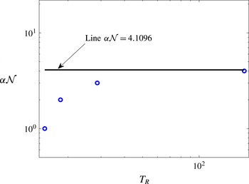
. Figure 5 displays the parameter
 $\unicode[STIX]{x1D6FC}{\mathcal{N}}$
as a function of rupture time
 $T_{R}$
by performing Fourier spectral simulations of (5.1). As
 $\unicode[STIX]{x1D6FC}{\mathcal{N}}$
approaches the horizontal line at
 $4.1096$
, the rupture time
 $T_{R}$
increases and past this point becomes infinite. Figure 5 shows an excellent agreement between numerical simulations and the theoretical analysis leading to (5.7).
When
 $\unicode[STIX]{x1D702}^{\prime }=0$
the corresponding critical value is
 $$\begin{eqnarray}{\mathcal{N}}^{\ast }=2\sqrt{38}(1-\unicode[STIX]{x1D6FC})/\unicode[STIX]{x1D6FC}\sim 12.33(1-\unicode[STIX]{x1D6FC})/\unicode[STIX]{x1D6FC},\end{eqnarray}$$
and the dimensional torque density critical value will be
 $N^{\ast }=4\sqrt{38}\unicode[STIX]{x1D702}U_{0}/\unicode[STIX]{x1D709}_{0}$
. A numerical analysis of (2.1) can also be carried out to obtain a figure similar to figure 5 but with a horizontal asymptote for
 $(\unicode[STIX]{x1D6FC}/(1-\unicode[STIX]{x1D6FC})){\mathcal{N}}^{\ast }=12.33$
(see also figure 6 of Kirkinis & Davis Reference Kirkinis and Davis2015).
It is worth pointing out that an analogous study can be carried out for the evolution equation incorporating the full flux function (4.24), although the results obtained by such an analysis become less transparent when compared to the foregoing discussion.
Parameter
 $\unicode[STIX]{x1D6FC}{\mathcal{N}}$
as a function of rupture time
 $T_{R}$
by performing Fourier spectral simulations of (5.1). As
 ${\mathcal{N}}$
approaches the critical value
 ${\mathcal{N}}^{\ast }=4.1096/\unicode[STIX]{x1D6FC}$
, rupture times increase to infinity, in agreement with the theoretical analysis leading to (5.7).

6 Discussion
In this article we introduced a new physical effect in the evolution of thin liquid films endowed with rotational degrees of freedom: the collective particle rotation at a free surface competes with the instability-inducing mechanism (here this is the van der Waals attraction of the liquid–gas and liquid–solid interfaces) leading to a permanent coherent interfacial capillary–viscous wave. Thus, film rupture and substrate dewetting are both averted.
Apart from their fundamental importance, the mechanisms at play here and the corresponding theoretical analysis can shed light on recent experiments of ferrofluid flow counter-rotating with respect to a rotating magnetic field (Chaves et al. Reference Chaves, Zahn and Rinaldi2008). In these experiments one should expect that at the liquid–gas interface there will be a competition between a magnetic body force and the magnetic torque each driving the flow in opposite directions. Further, it is easy to show that, within the present framework, such competition can lead the interface and the bulk to flow in opposite directions which has also been observed in experiment. A three-dimensional counterpart of the present framework that would replace the intermolecular potential with gravity could in principle be employed to capture the essence of these effects. This is beyond the scope of the present article however.
Finally, the framework developed in this article can be employed in the study of suspensions of chiral particles and chiral molecules (Andreev, Son & Spivak Reference Andreev, Son and Spivak2010; Kirkinis et al. Reference Kirkinis, Andreev and Spivak2012). The stress and couple-stress tensors as well as the chiral current then acquire new terms depending, to leading order, on the imbalance between the polar particle angular velocity and liquid vorticity. Physically, this behaviour arises due to the microvortices induced by the collective rotation of the magnetic grains in one direction that tend to rotate the chiral particles in the opposite direction and thus translate them according to their handedness. This new chiral current exerts forces and torques on the base liquid. For Poiseuille flow in a duct, new chiral stresses arise that give rise to a force density and a resulting chiral velocity component perpendicular to the duct Poiseuille flow direction.
Acknowledgements
The author is grateful to S. H. Davis and A. V. Andreev for comments and advice that significantly improved the manuscript and to B. Z. Spivak, J. J. Riley and R. E. O’Malley, Jr. for helpful discussions. Also to the anonymous referees that provided suggestions and criticism during the review process.
Appendix A. The effect of the magnetic body force
Apart from the magnetic torque-induced effect described in this article, a body force
 $\boldsymbol{f}$
of magnetic origin may also arise but its effects are subdominant to those associated with the torque in the frequency range displayed in figure 3. In principle, this force is of the form
 $\boldsymbol{f}=(\boldsymbol{m}\boldsymbol{\cdot }\unicode[STIX]{x1D735})\boldsymbol{h}$
and must be superposed on the Navier–Stokes equations. It is not difficult to show that in the long wavelength limit and the geometry employed in this article, the time-averaged force points in the
 $z$
-direction and is of the form
 $\langle f_{3}\rangle \sim \unicode[STIX]{x2202}_{z}|m_{3}|^{2}$
(see also Zahn & Greer (Reference Zahn and Greer1995) (19)). The pressure
 $\bar{P}$
that enters the expression for the evolution equation of the liquid–gas interface acquires a new term proportional to
 $-|M_{3}|^{2}$
. In the slow rotation limit
 $M_{3}$
is approximately a constant that, in general, depends on the field frequency
 $\unicode[STIX]{x1D708}$
and amplitude, relaxation time
 $t_{s}$
and magnetic susceptibility
 $\unicode[STIX]{x1D712}$
and makes no contribution to the dynamics (in this regime).
Appendix B. Magnetic and magnetization fields
Equation (3.4) becomes
 $m_{1,t}+um_{1,x}+wm_{1,z}-\unicode[STIX]{x1D714}m_{3}+[m_{1}-\unicode[STIX]{x1D712}h_{1}]/t_{s}=0$
and
 $m_{3,t}+um_{3,x}+wm_{3,z}+\unicode[STIX]{x1D714}m_{1}+[m_{3}-\unicode[STIX]{x1D712}h_{3}]/t_{s}=0$
, while Maxwell’s equations read
 $h_{1,z}-h_{3,z}=0$
and
 $b_{1,x}+b_{3,z}=0$
. In the long wavelength approximation they take the form
 $$\begin{eqnarray}\displaystyle & \displaystyle 2\unicode[STIX]{x03C0}\text{i}\bar{\unicode[STIX]{x1D708}}\hat{M}_{1}+\unicode[STIX]{x1D716}[\hat{M}_{1,T}+U\hat{M}_{1,X}+W\hat{M}_{1,Z}]-\unicode[STIX]{x1D6FA}\hat{M}_{3}+[\hat{M}_{1}-{\hat{H}}_{1}]/\bar{\unicode[STIX]{x1D70F}}=0, & \displaystyle\end{eqnarray}$$
 $$\begin{eqnarray}\displaystyle & \displaystyle 2\unicode[STIX]{x03C0}\text{i}\bar{\unicode[STIX]{x1D708}}\hat{M}_{3}+\unicode[STIX]{x1D716}[\hat{M}_{3,T}+U\hat{M}_{3,X}+W\hat{M}_{3,Z}]+\unicode[STIX]{x1D6FA}\hat{M}_{1}+[\hat{M}_{3}-{\hat{H}}_{3}]/\bar{\unicode[STIX]{x1D70F}}=0, & \displaystyle\end{eqnarray}$$
and
 $H_{1,Z}-\unicode[STIX]{x1D716}H_{3,X}=0$
,
 $\unicode[STIX]{x1D716}B_{1,X}+B_{3,Z}=0$
. The first term on the right-hand side of both (B 1) and (B 2) arises because the magnetization field evolves on two separate time scales. The slow time scale
 $T\sim \unicode[STIX]{x1D716}t$
and the ‘fast’ time scale
 $U_{0}t/\unicode[STIX]{x1D709}_{0}$
which is here associated with the driving frequency
 $\bar{\unicode[STIX]{x1D708}}=\unicode[STIX]{x1D708}\unicode[STIX]{x1D709}_{0}/U_{0}$
of the external magnetic field:
 $M_{i}=\hat{M}_{i}(X,Z,T)\text{e}^{2\unicode[STIX]{x03C0}\text{i}\unicode[STIX]{x1D708}t}+\text{c.c.}$
,
 $i=1,3$
. This dependence arises from the corresponding time dependence of the magnetic and induction fields:
 $(H_{1},H_{3},B_{1},B_{3})=({\hat{H}}_{1},{\hat{H}}_{3}(X,Z,T),\hat{B}_{1}(X,Z,T),\hat{B}_{3})\text{e}^{2\unicode[STIX]{x03C0}\text{i}\unicode[STIX]{x1D708}t}+\text{c.c}$
. The third time scale
 $\bar{\unicode[STIX]{x1D70F}}=U_{0}t_{s}/\unicode[STIX]{x1D709}_{0}$
is here considered finite in the context of the long wavelength theory. To determine the distribution of magnetization we solve the linear system (4.20) for
 $M_{1}$
and
 $M_{2}$
and substitute into the time-averaged torque equation (4.23). The expressions are identical to those of Zahn & Greer (Reference Zahn and Greer1995) with a suitable adjustment of the axes.
Appendix C. The effect of slip and surface shear ‘wind’
In the presence of slip at the liquid–solid interface (Dussan V Reference Dussan V1976) and shear ‘wind’ at the liquid–gas interface (Davis et al. Reference Davis, Gratton and Davis2010), the first of the boundary conditions (4.16) and the first of (4.22) are replaced by
 $$\begin{eqnarray}U=\ell U_{Z}\quad \text{at }Z=0,\quad \text{and}\quad U_{Z}-2\unicode[STIX]{x1D6FC}\unicode[STIX]{x1D6FA}=\unicode[STIX]{x1D70F}\quad \text{at }Z=\unicode[STIX]{x1D6EF}(X,T),\end{eqnarray}$$
respectively, where
 $\ell$
and
 $\unicode[STIX]{x1D70F}$
are constant dimensionless parameters of slip length and shear stress respectively. It is then not difficult to show that the counterpart of the full nonlinear flux function (4.24) in the asymptotic limit of vanishing film thickness becomes
 $$\begin{eqnarray}\displaystyle \hspace{-23.00006pt}\int _{0}^{\unicode[STIX]{x1D6EF}}\!U\,\text{d}Z & = & \displaystyle \ell \unicode[STIX]{x1D70F}\unicode[STIX]{x1D6EF}+\left(-\bar{P}_{X}\ell +\frac{\unicode[STIX]{x1D70F}}{2}\right)\unicode[STIX]{x1D6EF}^{2}-\frac{1}{3}\bar{P}_{X}\unicode[STIX]{x1D6EF}^{3}\nonumber\\ \displaystyle \hspace{-23.00006pt} & & \displaystyle +\,\frac{\unicode[STIX]{x1D6FC}}{4}(\unicode[STIX]{x1D6FD}\unicode[STIX]{x1D70F}+{\mathcal{N}})\unicode[STIX]{x1D6EF}^{4}-\frac{\unicode[STIX]{x1D6FC}\unicode[STIX]{x1D6FD}}{10}\bar{P}_{X}\unicode[STIX]{x1D6EF}^{5}-\frac{7\unicode[STIX]{x1D6FC}\unicode[STIX]{x1D6FD}(1-\unicode[STIX]{x1D6FC})}{36}(\unicode[STIX]{x1D6FD}\unicode[STIX]{x1D70F}+{\mathcal{N}})\unicode[STIX]{x1D6EF}^{6}+O(\unicode[STIX]{x1D6EF}^{7}),\end{eqnarray}$$
and this replaces (4.25). The first three terms of the right-hand side are those expected on the basis of the standard lubrication theory (Oron et al. Reference Oron, Davis and Bankoff1997). All higher-order terms are new. This analysis shows that a surface shear ‘wind’ can enhance or compete against the magnetic torque thus forming a separate mechanism generating the rotation–counter-rotation observation in a ferrofluid (Chaves et al. Reference Chaves, Zahn and Rinaldi2008).