1 Introduction
The prediction of the skin-friction coefficient
 $c_{f}$
in compressible boundary layers is critically important for the design of high-speed vehicles and propulsion systems. The boundary-layer transition has a strong influence on aerodynamic drag and heating, because much higher friction and heating can be generated on the surface of aerospace vehicles in turbulent flows than those in laminar flows. Despite considerable efforts in theoretical, experimental and numerical studies, the reliable prediction of the skin-friction coefficient in compressible boundary layers is still very challenging (Zhong & Wang Reference Zhong and Wang2012).
The theoretical study of the empirical formula of
 $c_{f}$
in compressible boundary layers, in general, is restricted to the laminar or fully developed turbulent state. The empirical formulae of
 $c_{f}$
for compressible laminar and turbulent boundary layers are transformed from their counterparts in incompressible boundary layers (van Driest Reference van Driest1952, Reference van Driest1956; Spalding & Chi Reference Spalding and Chi1964; White & Christoph Reference White and Christoph1972). However, there is a lack of theoretical models for
 $c_{f}$
for the laminar–turbulent transition stage. The existing approximate models for predicting transition, such as the
 $e^{N}$
-method and parabolized stability equations (Herbert Reference Herbert1997), rely on empirical input or specific initial and inlet boundary conditions.
For the experimental study, it is extremely difficult to accurately measure
 $c_{f}$
in compressible boundary layers using direct or indirect methods. The direct methods employ a movable element, such as a piezoelectric element (Holden Reference Holden1972; Goyne, Stalker & Paull Reference Goyne, Stalker and Paull2003), to measure the skin-friction force acting on the surface. Nonetheless, the viscous forces compared with other forces are too small to be accurately measured in practice (Schetz Reference Schetz2010). The indirect methods generally measure skin-friction related quantities, and then calculate the skin friction from some analogy or data correlation. For example,
 $c_{f}$
can be indirectly determined from the mean velocity profile in a turbulent boundary layer. Since the near-wall velocity measurements from hot-wire anemometry (Hutchins & Choi Reference Hutchins and Choi2002; Tay, Khoo & Chew Reference Tay, Khoo and Chew2012) and particle image velocimetry (PIV) (He et al.
Reference He, Yi, Zhao, Tian and Chen2011a
; Zhu et al.
Reference Zhu, Yuan, Zhang and Lee2013) are still challenging in high-speed boundary layers, various extrapolation methods from different parts of the mean velocity profile measured in experiments have been proposed (see table 1 in Rodriguez-Lopez, Bruce & Buxton Reference Rodriguez-Lopez, Bruce and Buxton2015). Therefore, no universal method for the measurement of the local skin friction exists, and in each case a proper selection of the appropriate instrumentation has to be made from available direct and indirect methods (Hakkinen Reference Hakkinen2004).
For the numerical simulation of compressible boundary-layer transition, direct numerical simulation (DNS) is useful for understanding the transition mechanism and evaluating transition-prediction models (Zhong & Wang Reference Zhong and Wang2012), but it is computationally expensive, so it is restricted to low and moderate Reynolds numbers. The large-eddy simulation (LES) significantly reduces the computational cost by filtering small-scale motions and modelling the effect of subgrid-scale motion on large-scale motion, but its accuracy in the transition prediction is influenced by the resolution of the grids or the wall treatment (Ducros, Comte & Lesieur Reference Ducros, Comte and Lesieur1996). The method of Reynolds-averaged Navier–Stokes (RANS) equations with low computational cost usually requires a priori information of the transition point, so it has not been a complete predictive tool (see Walters & Cokljat Reference Walters and Cokljat2008; Wang & Fu Reference Wang and Fu2009; Durbin Reference Durbin2018). Moreover, the progress of the transition can be characterized by an intermittency factor (Emmons Reference Emmons1951; Dhawan & Narasimha Reference Dhawan and Narasimha1958), and it has been used in the transition models for both RANS (e.g. Suzen & Huang Reference Suzen and Huang2000; Menter, Langtry & Völker Reference Menter, Langtry and Völker2006) and LES (e.g. Zhao et al. Reference Zhao, Xia, Shi, Xiao and Chen2014).
The rapidly increasing
 $c_{f}$
in the transitional stage appears to coincide with the emergence of coherent structures (Fukagata, Iwamoto & Kasagi Reference Fukagata, Iwamoto and Kasagi2002; Sayadi et al.
Reference Sayadi, Schmid, Nichols and Moin2014; Zhao et al.
Reference Zhao, Xiong, Yang and Chen2018). The structures can be visualized by experimental imaging methods employing dye (Falco Reference Falco1977; Head & Bandyopadhyay Reference Head and Bandyopadhyay1981), hydrogen bubbles (Kline et al.
Reference Kline, Reynolds, Schraub and Runstadler1967; Lee & Wu Reference Lee and Wu2008) and small droplets (Smith & Smits Reference Smith and Smits1995). Furthermore, the recently developed nanoparticle-based planar laser scattering (NPLS) can visualize clear coherent structures in supersonic boundary-layer transition (He et al.
Reference He, Yi, Zhao, Tian and Chen2011b
; Wang, Wang & Zhao Reference Wang, Wang and Zhao2016; Wang et al.
Reference Wang, Wang, Sun, Yang, Zhao and Hu2019). Similar to the passive scalar used in the experimental imaging, the Lagrangian scalar field, as an ideal passive tracer field with vanishing diffusivity, is applied to study structural evolution in isotropic turbulence (Yang, Pullin & Bermejo-Moreno Reference Yang, Pullin and Bermejo-Moreno2010), Taylor–Green and Kida–Pelz flows (Yang & Pullin Reference Yang and Pullin2010), the K-type transition in channel flows (Zhao, Yang & Chen Reference Zhao, Yang and Chen2016), fully developed channel flows (Yang & Pullin Reference Yang and Pullin2011) and the transition in a weakly compressible boundary layer (Zheng, Yang & Chen Reference Zheng, Yang and Chen2016). The Lagrangian field is governed by a pure scalar advection equation and has no smallest scale, so it can reveal rich geometries of flow structures.
The visualization of scalar-like structures (e.g. Smith & Smits Reference Smith and Smits1995; He et al.
Reference He, Yi, Zhao, Tian and Chen2011b
) illustrates that the coherent, inclined structures emerge in the transitional stage and rapidly break down into multi-scale structures with different inclination angles, and the multi-scale geometry of the structures reaches a statistically stationary state in the fully developed turbulent state (Zheng et al.
Reference Zheng, Yang and Chen2016). For example, the inclination angle of the signature hairpin-like structures is close to
 $45^{\circ }$
(e.g. Head & Bandyopadhyay Reference Head and Bandyopadhyay1981; Spina, Donovan & Smits Reference Spina, Donovan and Smits1991; Adrian Reference Adrian2007; Yang & Pullin Reference Yang and Pullin2011). The evolutionary geometry of coherent structures with different scales and inclination angles in the laminar–turbulent transition is sketched in figure 1, along with the rise of
 $c_{f}$
. The superposition of hierarchies of attached and inclined vortical structures is also suggested by the models (e.g. Perry & Chong Reference Perry and Chong1982; Marusic & Monty Reference Marusic and Monty2019) based on the attached eddy hypothesis (Townsend Reference Townsend1976).
Evolutionary geometry of vortical or scalar structures, sketched by the ellipses with different scales and inclination angles, in the boundary-layer transition, along with the rise of the skin-friction coefficient
 $c_{f}$
.

On the other hand, the study of coherent structures is also criticized owing to the lack of quantitative results (see Robinson Reference Robinson1991), so that it is hard to develop predictive models from the findings on structures. In order to quantify the evolutionary, multi-scale and multi-directional geometry of flow structures in transitional flows, Zheng et al. (Reference Zheng, Yang and Chen2016) developed a diagnostic tool characterizing evolving scalar fields at different scales and evolutional stages during the transition. The diagnostic tool incorporates the tracking of the Lagrangian scalar field (Yang et al. Reference Yang, Pullin and Bermejo-Moreno2010), the multi-scale and multi-directional geometric analysis (Yang & Pullin Reference Yang and Pullin2011) based on the mirror-extended curvelet transform (Candes et al. Reference Candes, Demanet, Donoho and Ying2006) and a sliding window for extracting scalar fields at different locations in the transition.
In the present study, we develop a simple model of the skin-friction coefficient
 $c_{f}$
based on the multi-scale and multi-directional analysis of two-dimensional scalar images in compressible boundary-layer transition, considering that the scalar images are relatively easy to obtain in experiments by imaging techniques. We also aim to partially bridge the gap between the qualitative study of coherent structures and the predictive tool in applications of supersonic and hypersonic boundary layers.
We begin from § 2 as an overview of numerical implementations for the DNS of compressible boundary layers, Lagrangian scalar tracking and multi-scale diagnostic methodology. Section 3 presents the application of the diagnostic method for investigating the evolutionary inclination angles in the transition, and § 4 proposes and validates the model of
 $c_{f}$
based on the statistics of structural inclination angles on the streamwise and wall-normal plane at different scales. We draw some conclusions in § 5.
2 Simulation overview
2.1 DNS
The DNS of the spatially evolving flat-plate boundary layer is performed by solving the three-dimensional compressible Navier–Stokes (N–S) equations
 $$\begin{eqnarray}\frac{\unicode[STIX]{x2202}\boldsymbol{U}}{\unicode[STIX]{x2202}t}+\frac{\unicode[STIX]{x2202}\boldsymbol{F}_{j}}{\unicode[STIX]{x2202}x_{j}}-\frac{\unicode[STIX]{x2202}\boldsymbol{V}_{j}}{\unicode[STIX]{x2202}x_{j}}=0,\end{eqnarray}$$
with
 $$\begin{eqnarray}\boldsymbol{U}=\left(\begin{array}{@{}c@{}}\unicode[STIX]{x1D70C}\\ \unicode[STIX]{x1D70C}u_{1}\\ \unicode[STIX]{x1D70C}u_{2}\\ \unicode[STIX]{x1D70C}u_{3}\\ E\end{array}\right),\quad \boldsymbol{F}_{j}=\left(\begin{array}{@{}c@{}}\unicode[STIX]{x1D70C}u_{j}\\ \unicode[STIX]{x1D70C}u_{1}u_{j}+p\unicode[STIX]{x1D6FF}_{1j}\\ \unicode[STIX]{x1D70C}u_{2}u_{j}+p\unicode[STIX]{x1D6FF}_{2j}\\ \unicode[STIX]{x1D70C}u_{3}u_{j}+p\unicode[STIX]{x1D6FF}_{3j}\\ (E+p)u_{j}\end{array}\right),\quad \boldsymbol{V}_{j}=\left(\begin{array}{@{}c@{}}0\\ \unicode[STIX]{x1D70E}_{1j}\\ \unicode[STIX]{x1D70E}_{2j}\\ \unicode[STIX]{x1D70E}_{3j}\\ \unicode[STIX]{x1D70E}_{jk}u_{k}+\unicode[STIX]{x1D705}\displaystyle \frac{\unicode[STIX]{x2202}T}{\unicode[STIX]{x2202}x_{j}}\end{array}\right).\end{eqnarray}$$
Here, the Einstein summation is used, and the subscript
 $j=1,2,3$
denotes the index in three-dimensional Cartesian coordinates. The coordinates
 $x_{1}$
,
 $x_{2}$
and
 $x_{3}$
are equivalent to
 $x$
,
 $y$
and
 $z$
, respectively. The velocity components are denoted by
 $u_{j}$
in the
 $j$
th coordinate direction, or
 $u$
,
 $v$
and
 $w$
in the
 $x$
,
 $y$
and
 $z$
directions, respectively;
 $\unicode[STIX]{x1D70C}$
is the density,
 $p$
the static pressure,
 $\unicode[STIX]{x1D6FF}_{ij}$
the Kronecker delta function,
 $\unicode[STIX]{x1D705}$
the thermal conductivity and
 $T$
the temperature. The N–S equations (2.1) are non-dimensionalized with the free-stream quantities
 $\unicode[STIX]{x1D70C}_{\infty }$
,
 $T_{\infty }$
,
 $U_{\infty }$
and
 $\unicode[STIX]{x1D707}_{\infty }$
. The length and time scales are non-dimensionalized by the reference length
 $L=1$
inch and time
 $L/U_{\infty }$
, respectively.
It is noted that the subscript ‘
 $\infty$
’ denotes the free-stream properties, and ‘
 $w$
’ denotes the quantities on the wall. The free-stream Mach number is
 $Ma_{\infty }\equiv U_{\infty }/c_{\infty }$
where
 $c_{\infty }$
is the free-stream sound speed. The free-stream Reynolds number is
 $Re_{\infty }\equiv \unicode[STIX]{x1D70C}_{\infty }U_{\infty }L/\unicode[STIX]{x1D707}_{\infty }$
, and the wall temperature
 $T_{w}$
is normalized by the free-stream temperature
 $T_{\infty }=169.4$
K.
In the perfect gas assumption, the total energy is
 $$\begin{eqnarray}E=\unicode[STIX]{x1D70C}c_{v}T+{\textstyle \frac{1}{2}}\unicode[STIX]{x1D70C}u_{i}u_{i},\end{eqnarray}$$
where
 $c_{v}$
is the specific heat at constant volume. For a compressible Newtonian flow, the viscous stress is
 $$\begin{eqnarray}\unicode[STIX]{x1D70E}_{ij}=\unicode[STIX]{x1D707}\left(\frac{\unicode[STIX]{x2202}u_{i}}{\unicode[STIX]{x2202}x_{j}}+\frac{\unicode[STIX]{x2202}u_{j}}{\unicode[STIX]{x2202}x_{i}}\right)-\frac{2}{3}\unicode[STIX]{x1D707}\frac{\unicode[STIX]{x2202}u_{k}}{\unicode[STIX]{x2202}x_{k}}\unicode[STIX]{x1D6FF}_{ij},\end{eqnarray}$$
where the dynamic viscosity
 $\unicode[STIX]{x1D707}$
is assumed to obey Sutherland’s law.
As shown in figure 2, the computational domain is bounded by an inlet boundary and a non-reflecting outlet boundary in the streamwise
 $x$
-direction, a wall boundary and a non-reflecting upper boundary in the wall-normal
 $y$
-direction and two periodic boundaries in the spanwise
 $z$
-direction. The inlet boundary is given by a laminar compressible boundary-layer similarity solution. The wall temperature is prescribed by an approximate adiabatic (or recovery) temperature
 $$\begin{eqnarray}T_{w}=1+r\frac{\unicode[STIX]{x1D6FE}-1}{2}Ma_{\infty }^{2},\end{eqnarray}$$
so that the wall can be considered as quasi-isothermal (see Duan, Beekman & Martin Reference Duan, Beekman and Martin2010). Here,
 $\unicode[STIX]{x1D6FE}=1.4$
denotes the ratio of specific heats at constant pressure and volume, and
 $r=Pr^{1/3}$
denotes the flat-plate turbulent recovery factor (see White Reference White2006) with the Prandtl number
 $Pr=0.72$
.
A schematic diagram of the computational domain with boundary conditions. The inclined structure is sketched by the dashed line with the inclination angle
 $\unicode[STIX]{x1D6FC}$
.

In order to trigger the laminar–turbulent transition, a region of blowing and suction at
 $x_{a}\leqslant x\leqslant x_{b}$
is imposed. The wall-normal disturbing velocity is generated as (see Pirozzoli, Grasso & Gatski Reference Pirozzoli, Grasso and Gatski2004; Gao et al.
Reference Gao, Fu, Ma and Li2005)
 $$\begin{eqnarray}v_{bs}(x,z,t)=Af(x)g(z)h(t),\quad x_{a}\leqslant x\leqslant x_{b}.\end{eqnarray}$$
Here,
 $A$
is the amplitude of disturbance, and the functions are
 $$\begin{eqnarray}\displaystyle \left.\begin{array}{@{}c@{}}f(x)=4\sin \unicode[STIX]{x1D6E9}(1-\cos \unicode[STIX]{x1D6E9})/\sqrt{27},\\ \unicode[STIX]{x1D6E9}=2\unicode[STIX]{x03C0}(x-x_{a})/(x_{a}-x_{b}),\end{array}\right\} & & \displaystyle\end{eqnarray}$$
 $$\begin{eqnarray}\displaystyle \left.\begin{array}{@{}c@{}}\displaystyle g(z)=\mathop{\sum }_{l=1}^{l_{max}}Z_{l}\sin [2\unicode[STIX]{x03C0}l(z/L_{z}+\unicode[STIX]{x1D719}_{l})],\\ \displaystyle \mathop{\sum }_{l=1}^{l_{max}}Z_{l}=1,\quad Z_{l}=1.25Z_{l+1},\end{array}\right\} & & \displaystyle\end{eqnarray}$$
 $$\begin{eqnarray}\displaystyle \left.\begin{array}{@{}c@{}}\displaystyle h(t)=\mathop{\sum }_{m=1}^{m_{max}}T_{m}\sin [2\unicode[STIX]{x03C0}(m\unicode[STIX]{x1D6FD}t+\unicode[STIX]{x1D719}_{m})],\\ \displaystyle \mathop{\sum }_{m=1}^{m_{max}}T_{m}=1,\quad T_{m}=1.25T_{m+1},\end{array}\right\} & & \displaystyle\end{eqnarray}$$
where
 $L_{z}$
is the size of the computational domain in the spanwise direction,
 $\unicode[STIX]{x1D6FD}$
is the base frequency of disturbance,
 $\unicode[STIX]{x1D719}_{l}$
and
 $\unicode[STIX]{x1D719}_{m}$
are random numbers ranging from 0 to 1 and
 $l_{max}=10$
and
 $m_{max}=5$
are maximum numbers of disturbing modes. In general, the transition is delayed by decreasing
 $A$
, and the transitional region is extended and the overshoot of
 $c_{f}$
at the end of transition is diminished by decreasing
 $\unicode[STIX]{x1D6FD}$
.
The DNS is implemented using the OpenCFD code (Li, Fu & Ma Reference Li, Fu and Ma2010), which has been widely used and validated in compressible transitional and turbulent flows (see Li et al.
Reference Li, Fu and Ma2010; Zhang et al.
Reference Zhang, Bi, Hussain and She2014; Zheng et al.
Reference Zheng, Yang and Chen2016). The N–S equations (2.1) are integrated in time by using the third-order total-variation-diminishing-type Runge–Kutta method. The convection terms
 $\unicode[STIX]{x2202}\boldsymbol{F}_{j}/\unicode[STIX]{x2202}x_{j}$
are approximated by a seventh-order weighted essentially non-oscillatory scheme (Jiang & Shu Reference Jiang and Shu1996), and the viscous terms
 $\unicode[STIX]{x2202}\boldsymbol{V}_{j}/\unicode[STIX]{x2202}x_{j}$
are approximated by an eighth-order central finite-difference scheme.
In the present DNS, two Mach numbers are considered, and the parameters are listed in table 1. The computational domain with size
 $L_{x}\times L_{y}\times L_{z}$
is discretized using grid points
 $N_{x}\times N_{y}\times N_{z}$
with grid spacing
 $\unicode[STIX]{x0394}x\times \unicode[STIX]{x0394}y\times \unicode[STIX]{x0394}z$
. The superscript ‘
 $+$
’ denotes a quantity normalized by a wall unit (Robinson Reference Robinson1991), i.e. the viscous length scale
 $\unicode[STIX]{x1D6FF}_{\unicode[STIX]{x1D708}}\equiv \unicode[STIX]{x1D707}_{w}/(\unicode[STIX]{x1D70C}_{w}u_{\unicode[STIX]{x1D70F}})$
or the friction velocity
 $u_{\unicode[STIX]{x1D70F}}\equiv \sqrt{\unicode[STIX]{x1D70F}_{w}/\unicode[STIX]{x1D70C}_{w}}$
with the wall shear stress
 $\unicode[STIX]{x1D70F}_{w}$
in the fully developed turbulent region. Moreover, the real-gas effect is not considered as in previous low-enthalpy DNS studies (e.g. Pirozzoli et al.
Reference Pirozzoli, Grasso and Gatski2004; Duan, Beekman & Martin Reference Duan, Beekman and Martin2011; Zhang et al.
Reference Zhang, Bi, Hussain and She2014).
DNS parameters.

Table 2 summarizes the Mach number, Reynolds number
 $Re_{\unicode[STIX]{x1D703}}\equiv Re_{\infty }\unicode[STIX]{x1D703}$
based on the momentum thickness
 $\unicode[STIX]{x1D703}$
and grid resolution in wall units in recent DNS of compressible transitional and turbulent boundary layers. The grid resolution of the present study is comparable to those in recent DNS studies.
Parameters and grid resolutions in recent DNS of compressible boundary layers.

The computational domain is partitioned into four zones in the streamwise direction to reduce the computational cost. The range and number of grid points in the streamwise direction of each computational zone are listed in table 3. A coarse grid is used in the first laminar zone, containing the region of blowing and suction from
 $x_{a}=0.5$
to
 $x_{b}=1.0$
and a small fraction of the transition region. A fine grid is used in the third turbulent zone, where the flow has reached the fully developed turbulent state. A stretched grid is applied to the second transition zone to smoothly transform the coarse grid to the fine grid. A gradually coarser grid is used in the fourth sponge zone to minimize the numerical error generated by the outlet boundary condition. In the wall-normal direction, exponentially stretched grid points
 $$\begin{eqnarray}y_{j}=L_{y}\frac{\tanh [b((j-1)/(N_{y}-1)-1)]}{\tanh b}+L_{y},\quad j=1,2,\ldots ,N_{y},\end{eqnarray}$$
with
 $b=2.93$
, are applied to capture small-scale structures near the wall. A uniform grid is applied in the spanwise direction.
The range and number of grid points in the streamwise direction for four computational zones in DNS.

The present DNS results are validated by theoretical and existing numerical results in figure 3. The mean flow statistics in the fully developed turbulent region from DNS in figure 3(a) agree well with the DNS results in Pirozzoli et al. (Reference Pirozzoli, Grasso and Gatski2004). Figure 3(b) shows that the van Driest transforms of the normalized mean velocity profiles satisfy the theoretical fits in the viscous sublayer and the logarithm law region. Figure 4(a) shows that the skin-friction coefficient
 $c_{f}\equiv \unicode[STIX]{x1D70F}_{w}/(\frac{1}{2}\unicode[STIX]{x1D70C}_{\infty }U_{\infty }^{2})$
along the streamwise direction from DNS agrees well with the empirical formulae of
 $c_{f}$
in the laminar and fully developed turbulent regions. Here, the formula for the compressible laminar skin friction is
 $$\begin{eqnarray}c_{fL}(x)=\frac{0.664}{\sqrt{Re_{x}^{\ast }}},\end{eqnarray}$$
with
 $Re_{x}^{\ast }=\unicode[STIX]{x1D70C}^{\ast }U_{\infty }x/\unicode[STIX]{x1D707}^{\ast }$
(see Anderson Reference Anderson2010) at the reference temperature
 $$\begin{eqnarray}T^{\ast }=1+0.032Ma_{\infty }^{2}+0.58(T_{w}-1).\end{eqnarray}$$
The formula for the compressible turbulent skin friction is
 $$\begin{eqnarray}c_{fT}(x)=\frac{0.455}{S^{2}}\left[\ln \left(\frac{0.06}{S}Re_{x}\frac{1}{\unicode[STIX]{x1D707}_{w}}\sqrt{\frac{1}{T_{w}}}\right)\right]^{-2},\end{eqnarray}$$
with
 $Re_{x}\equiv Re_{\infty }x$
,
 $S=\sqrt{T_{w}-1}/\sin ^{-1}{\mathcal{A}}$
and
 ${\mathcal{A}}=(r((\unicode[STIX]{x1D6FE}-1)/2)Ma_{\infty }^{2}(1/T_{w}))^{1/2}$
, which is accurate over the practical range of
 $Re_{\unicode[STIX]{x1D703}}$
,
 $Ma_{\infty }$
and
 $T_{w}$
(see White Reference White2006).
Validation of the present DNS result. (a) Mean profiles in the fully developed turbulent region at
 $Ma_{\infty }=2.25$
in the present DNS (lines) and in the DNS (symbols) by Pirozzoli et al. (Reference Pirozzoli, Grasso and Gatski2004). The overbar denotes the Reynolds average over the spanwise direction. (b) Normalized mean velocity profiles
 $\bar{u}^{+}$
(symbols) and their van Driest transforms
 $\bar{u}_{vd}=\int _{0}^{\bar{u}^{+}}(\bar{\unicode[STIX]{x1D70C}}/\bar{\unicode[STIX]{x1D70C}}_{w})^{1/2}\,\text{d}\bar{u}^{+}$
(solid and dashed lines) with theoretical fits
 $\bar{u}_{vd}=y^{+}$
in the viscous sublayer and
 $\bar{u}_{vd}=\ln y^{+}/0.41+5.5$
in the logarithm law region.

The skin-friction coefficient along the streamwise direction. Note the spatial coordinate is normalized by the reference length
 $L=1$
inch in DNS. (a) Comparison of DNS results and empirical formulae (2.11) and (2.13) at two Mach numbers. (b) Convergence of
 $c_{f}$
with three grid resolutions listed in table 1 at
 $Ma_{\infty }=6$
.

The rapid increase of
 $c_{f}$
signals the transition, and this appears to coincide with the generation of three-dimensional vortices and the breakdown of large-scale coherent structures. The transitional regions are roughly at
 $2\leqslant x\leqslant 4$
and
 $3\leqslant x\leqslant 5$
for
 $Ma_{\infty }=2.25$
and
 $Ma_{\infty }=6$
, respectively.
The grid convergence of the skin friction for
 $Ma_{\infty }=6$
is assessed using three different grid resolutions in figure 4(b). Since
 $c_{f}$
is converged for the moderate and fine grids, the moderate grids are used in the following study. Furthermore, we find that the tails of the two-point correlations of the velocity components in the spanwise direction are sufficiently small at lateral boundaries (not shown), which ensures that
 $L_{z}$
is large enough so that the imposed periodic boundary condition does not affect flow statistics (Pirozzoli et al.
Reference Pirozzoli, Grasso and Gatski2004).
2.2 Lagrangian scalar field
The three-dimensional Lagrangian scalar field
 $\unicode[STIX]{x1D719}(\boldsymbol{x},t)$
is an ideal passive tracer field, and isosurfaces of
 $\unicode[STIX]{x1D719}$
are material surfaces in the temporal evolution. The scalar field is governed by the pure convection equation
 $$\begin{eqnarray}\frac{\unicode[STIX]{x2202}\unicode[STIX]{x1D719}}{\unicode[STIX]{x2202}t}+\boldsymbol{u}\boldsymbol{\cdot }\unicode[STIX]{x1D735}\unicode[STIX]{x1D719}=0.\end{eqnarray}$$
Although
 $\unicode[STIX]{x1D719}$
is similar to the temperature or species concentration, it has no diffusivity so that it has no smallest scale in the evolution at long times. Thus it can display a rich geometry of flow structures at very fine scales, and excludes the subjective selection of the diffusivity value.
The backward-particle-tracking method (Yang et al. Reference Yang, Pullin and Bermejo-Moreno2010; Yang & Pullin Reference Yang and Pullin2011), which is numerically stable and has no numerical dissipation, is used to solve (2.14). In this method, trajectories of fluid particles are calculated by solving the kinematic equation
 $$\begin{eqnarray}\frac{\unicode[STIX]{x2202}\boldsymbol{X}(\boldsymbol{x}_{0},t_{0}|t)}{\unicode[STIX]{x2202}t}=\boldsymbol{V}(\boldsymbol{x}_{0},t_{0}|t)=\boldsymbol{u}(\boldsymbol{X}(\boldsymbol{x}_{0},t_{0}|t),t),\end{eqnarray}$$
where
 $\boldsymbol{X}(\boldsymbol{x}_{0},t_{0}|t)$
is the location at time
 $t$
of a fluid particle which was located at
 $\boldsymbol{x}_{0}$
at the initial time
 $t_{0}$
,
 $\boldsymbol{V}(\boldsymbol{x}_{0},t_{0}|t)$
is the Lagrangian velocity of the fluid particle and
 $\boldsymbol{u}(\boldsymbol{X}(\boldsymbol{x}_{0},t_{0}|t),t)$
is its local Eulerian velocity.
The initial Lagrangian field is uniquely determined as
 $\unicode[STIX]{x1D719}(\boldsymbol{x}_{0},t_{0})=y$
based on the criteria of the best approximation of vortex sheets and geometric invariance of
 $\unicode[STIX]{x1D719}$
in the laminar state (Zhao et al.
Reference Zhao, Yang and Chen2016). The isosurfaces of
 $\unicode[STIX]{x1D719}(\boldsymbol{x}_{0},t_{0})$
are streamwise–spanwise planes at different distances from the wall at the initial time. Near the inlet, the amplitudes of initial disturbances are very small compared to the mean flow, so that the material sheets are almost invariant. As the disturbances develop with increasing
 $x$
, the material surfaces are stretched and folded in the streamwise and wall-normal plane. Subsequently, some parts of the material surfaces can be rolled up into complex shapes with three-dimensional geometric characteristics in the evolution (Zhao et al.
Reference Zhao, Yang and Chen2016).
In the numerical implementation of the backward-particle-tracking method,
 $\unicode[STIX]{x1D719}$
at a given time
 $t$
is calculated as follows (Zheng et al.
Reference Zheng, Yang and Chen2016).
(i) The full Eulerian velocity field on the grid
 $N_{x}\times N_{y}\times N_{z}$
within a time period from
 $t_{0}$
to
 $t>t_{0}$
is solved by DNS and then stored to disk.
(ii) As sketched in figure 2, at the given time
 $t$
, particles are placed at uniform grid points of
 $N_{x}^{p}\times N_{y}^{p}$
in a subdomain of interest in a number of
 $x$
–
 $y$
planes for further geometric analysis. The time period
 $\unicode[STIX]{x0394}T\equiv t-t_{0}$
for the backward-particle tracking in the implementation is set to be
 $\unicode[STIX]{x0394}T=1$
following the selection argument in Zheng et al. (Reference Zheng, Yang and Chen2016). Numerical experiments demonstrate that the statistical results for
 $\unicode[STIX]{x1D719}$
are not sensitive to the value of
 $\unicode[STIX]{x0394}T\geqslant 1$
.
(iii) The particles are released and their trajectories are calculated backward in time within
 $\unicode[STIX]{x0394}T$
or until they arrive at
 $x_{0}=0.2$
where the initial material surfaces are considered as planar sheets. A three-dimensional, fourth-order Lagrangian interpolation scheme is used to obtain the fluid velocity at the location of each particle. An explicit, second-order Adams–Bashforth scheme is applied for the time integration, and time steps
 $\unicode[STIX]{x0394}t=0.0025$
for
 $Ma_{\infty }=2.25$
and
 $\unicode[STIX]{x0394}t=0.005$
for
 $Ma_{\infty }=6$
are selected by the criterion
 $\unicode[STIX]{x0394}t\leqslant \unicode[STIX]{x1D6FF}_{\unicode[STIX]{x1D708}}/u_{\unicode[STIX]{x1D70F}}$
for capturing the finest resolved scales in the velocity field.
(iv) After the backward tracking, we obtain initial locations
 $\boldsymbol{x}_{0}$
of the particles and the flow map
 $$\begin{eqnarray}F_{t}^{t_{0}}(\boldsymbol{X})\boldsymbol{ : }\boldsymbol{X}(\boldsymbol{x}_{0},t_{0}|t)\mapsto \boldsymbol{x}_{0},\quad t\geqslant t_{0}.\end{eqnarray}$$
Then the Lagrangian field
 $\unicode[STIX]{x1D719}(\boldsymbol{x},t)$
at any given time
 $t$
is obtained as
 $$\begin{eqnarray}\unicode[STIX]{x1D719}(\boldsymbol{x},t)=\unicode[STIX]{x1D719}(F_{t}^{t_{0}}(\boldsymbol{X}),t_{0}).\end{eqnarray}$$
2.3 Geometric diagnostic methodology
A systematic diagnostic tool has been developed to quantify the multi-scale geometry of flow structures in the transition of boundary layers (see Zheng et al. Reference Zheng, Yang and Chen2016). It is also a general signal processing method for characterizing preferential orientations in the scalar pattern of images from DNS (see § 3) and experiments (see appendix A).
First, a sliding window filter is used to extract the spatially evolving scalar structures and capture their major deformation in the compact frames at different streamwise locations. The filter is defined as
 $$\begin{eqnarray}f(x)=\exp \left[-n\left(\frac{x-x_{c}}{l_{w}}\right)^{n}\right],\end{eqnarray}$$
where
 $x_{c}$
is the position of the window centre,
 $l_{w}$
is a characteristic width of the window and
 $n$
is a positive even integer. Figure 5 illustrates the profile of the filter. From (2.18), the window width
 $l\equiv 2(x-x_{c})$
of the filter for a given
 $f$
is
 $$\begin{eqnarray}l=2\,l_{w}\exp \left[\frac{\ln (-\ln f/n)}{n}\right].\end{eqnarray}$$
The two-dimensional scalar field for further analysis is extracted in a compact region with the cutoff window width
 $l=l_{c}$
given
 $f=0.0001$
at the boundaries. The major features of the extracted scalar field with a large scalar gradient
 $\unicode[STIX]{x1D735}\unicode[STIX]{x1D719}$
are captured in the subdomain with the effective window width
 $l=l_{e}$
for
 $f\geqslant 0.9$
. As shown in figure 5, we choose
 $n=16$
to smooth the transition of
 $f$
from
 $f=0$
to
 $1$
with
 $l_{c}/l_{w}=1.93$
and
 $l_{e}/l_{w}=1.46$
.
The profile of the sliding window function for extracting
 $\unicode[STIX]{x1D719}_{f}$
from the entire
 $\unicode[STIX]{x1D719}$
.

Setting
 $l_{e}=1$
and given
 $x_{c}$
, the extracted Lagrangian scalar field
 $\unicode[STIX]{x1D719}_{f}(\boldsymbol{x},t)$
is obtained as
 $$\begin{eqnarray}\unicode[STIX]{x1D719}_{f}(\boldsymbol{x},t)=\unicode[STIX]{x1D719}(\boldsymbol{x},t)f+\unicode[STIX]{x1D719}(\boldsymbol{x}_{0},t_{0})(1-f).\end{eqnarray}$$
The extracted Lagrangian field in the sliding window has a smooth transition from an evolving scalar
 $\unicode[STIX]{x1D719}(\boldsymbol{x},t)$
to the initial scalar
 $\unicode[STIX]{x1D719}(\boldsymbol{x}_{0},t_{0})$
at lateral boundaries of the window, and the effect of this artificial transition on the further directional analysis is negligible. Thus the periodic boundary condition of
 $\unicode[STIX]{x1D719}_{f}$
in the
 $x$
-direction and the mirror extension of
 $\unicode[STIX]{x1D719}_{f}$
in the
 $y$
-direction can facilitate the fast Fourier transform of
 $\unicode[STIX]{x1D719}_{f}$
in further analysis without the numerical artefact due to possible discontinuities at the boundaries (Zheng et al.
Reference Zheng, Yang and Chen2016).
The multi-scale and multi-directional geometric analysis (Yang & Pullin Reference Yang and Pullin2011) is applied to characterize the evolutionary geometry of
 $\unicode[STIX]{x1D719}_{f}$
on a series of streamwise and wall-normal (
 $x$
–
 $y$
) planes. This provides quantitative statistics on the inclination angle of scalar structures in the images at different scales and streamwise locations during the transition.
The mechanism of the multi-scale and multi-directional geometric analysis is briefly explained here, and more details and illustrative examples can be found in Yang & Pullin (Reference Yang and Pullin2011). As sketched in figure 6(a), if a two-dimensional scalar field or image
 $\unicode[STIX]{x1D711}(\boldsymbol{x})\in \mathbb{R}^{2}$
has a characteristic scale and a preferential orientation, then the geometric features are quantified from its Fourier transform
 $\hat{\unicode[STIX]{x1D711}}(\boldsymbol{k})={\mathcal{F}}\{\unicode[STIX]{x1D711}(\boldsymbol{x})\}$
as follows.
A filtered
 $\unicode[STIX]{x1D711}(\boldsymbol{x})$
at scale
 $j$
and along direction
 $l$
can be obtained by the inverse Fourier transform of
 $\hat{\unicode[STIX]{x1D711}}(\boldsymbol{k})$
filtered by the frequency window function
 $U_{j}(r,\unicode[STIX]{x1D703})=2^{-3j/4}W(2^{-j}r)V(t_{l}(\unicode[STIX]{x1D703}))$
in polar coordinates
 $r=\sqrt{k_{1}^{2}+k_{2}^{2}}$
and
 $\unicode[STIX]{x1D703}=\arctan (k_{2}/k_{1})$
with
 $j\in \mathbb{N}$
. Here, the radial window function
 $W(r)$
and the angular window function
 $V(t_{l})$
are defined by explicit functions (Yang & Pullin Reference Yang and Pullin2011).
As illustrated in figure 6(b), each frequency window function in Fourier space is supported on the region of a circular wedge in the range of wavenumbers
 $2^{j-1}\leqslant r\leqslant 2^{j+1}$
with
 $j=0,1,\ldots ,j_{e}$
. This implies that the corresponding spatial structure in physical space is a needle-shaped element or a curvelet (Candes et al.
Reference Candes, Demanet, Donoho and Ying2006) with the characteristic length
 $2^{-j/2}$
and width
 $2^{-j}$
. Here,
 $j_{e}=\log _{2}[\min (k_{1,\max },k_{2,\max })/2]$
denotes the maximum number of scales, where
 $k_{1,\max }$
and
 $k_{2,\max }$
denote maximum resolved wavenumbers in the discrete Fourier transform of
 $\unicode[STIX]{x1D711}(\boldsymbol{x})$
.
Schematic plots of (a) the inclined structure with characteristic angle and scale in physical space and (b) frequency window functions
 $U_{j}(r,\unicode[STIX]{x1D703})$
supported on circular wedges in Fourier space with the region highlighted by the red circle for the characteristic angle and scale.

The multi-scale decomposition of
 $\unicode[STIX]{x1D711}(\boldsymbol{x})$
gives the filtered component field
 $\unicode[STIX]{x1D711}_{j}(\boldsymbol{x})={\mathcal{F}}^{-1}\{\hat{\unicode[STIX]{x1D711}}(\boldsymbol{k})W(2^{-j}r)\}$
with a characteristic length scale
 ${\mathcal{L}}_{j}=2^{-j}$
from the inverse Fourier transform, where the band-pass filter
 $W(r)$
is compact in Fourier space. In the boundary-layer transition, the normalized characteristic length scales of structures in the multi-scale decomposition are listed in table 4. Subsequently,
 ${\mathcal{L}}_{j}\geqslant 0.5\unicode[STIX]{x1D6FF}$
will be referred to as ‘large scale’,
 ${\mathcal{L}}_{j}\leqslant 50\unicode[STIX]{x1D6FF}_{\unicode[STIX]{x1D708}}$
as ‘small scale’ and in between as ‘intermediate scale’.
Characteristic length scales
 ${\mathcal{L}}_{j}$
normalized by the boundary-layer thickness
 $\unicode[STIX]{x1D6FF}$
and viscous length scale
 $\unicode[STIX]{x1D6FF}_{\unicode[STIX]{x1D708}}$
at
 $x=7$
.

The orientation information of each filtered component field of
 $\unicode[STIX]{x1D711}(\boldsymbol{x})$
is characterized by the normalized angular spectrum
 $$\begin{eqnarray}\unicode[STIX]{x1D6F7}_{j}(\unicode[STIX]{x0394}\unicode[STIX]{x1D703})=\frac{\displaystyle \int \hat{\unicode[STIX]{x1D711}}(\boldsymbol{k})U_{j}(r,\unicode[STIX]{x1D703})\,\text{d}\boldsymbol{k}}{\displaystyle \int U_{j}(r,\unicode[STIX]{x1D703})\,\text{d}\boldsymbol{k}},\quad -\frac{\unicode[STIX]{x03C0}}{2}\leqslant \unicode[STIX]{x0394}\unicode[STIX]{x1D703}\leqslant \frac{\unicode[STIX]{x03C0}}{2},\end{eqnarray}$$
where
 $\unicode[STIX]{x0394}\unicode[STIX]{x1D703}=\unicode[STIX]{x03C0}l^{\prime }2^{-\lceil j/2\rceil }/2$
,
 $-2^{\lceil j/2\rceil }\leqslant l^{\prime }\leqslant 2^{\lceil j/2\rceil }$
is the discrete deviation angle away from the
 $x$
-axis in the physical space for scale
 $j$
. As illustrated in figure 2, we define the inclination angle
 $\unicode[STIX]{x1D6FC}$
between an inclined structure projected onto the streamwise and wall-normal (
 $x$
–
 $y$
) plane and the
 $x$
-direction. The averaged inclination angle away from
 $x$
-axis at each scale
 $j$
is calculated by
 $$\begin{eqnarray}\langle \unicode[STIX]{x1D6FC}({\mathcal{L}}_{j})\rangle =\frac{\displaystyle \mathop{\sum }_{l^{\prime }=0}^{l_{\max }^{\prime }}\unicode[STIX]{x1D6F7}_{j}(\unicode[STIX]{x0394}\unicode[STIX]{x1D703})\unicode[STIX]{x0394}\unicode[STIX]{x1D703}}{\displaystyle \mathop{\sum }_{l^{\prime }=0}^{l_{\max }^{\prime }}\unicode[STIX]{x1D6F7}_{j}(\unicode[STIX]{x0394}\unicode[STIX]{x1D703})},\end{eqnarray}$$
with
 $l_{max}^{\prime }=2^{\lceil j/2\rceil }$
.
3 Scalar images on the streamwise and wall-normal plane
In the spatially developed boundary layer, the Lagrangian scalar field
 $\unicode[STIX]{x1D719}$
is calculated on
 $x$
–
 $y$
planes in the subdomain of interest within
 $L_{x1}\leqslant x\leqslant L_{x2}$
and
 $L_{y1}\leqslant y\leqslant L_{y2}$
, with
 $L_{x1}=0.5$
,
 $L_{x2}=6.5$
,
 $L_{y1}=0$
and
 $L_{y2}=0.3$
in the implementation. This subdomain encloses the transitional region and parts of laminar and turbulent regions. The numbers of grid points
 $N_{x}^{p}\times N_{y}^{p}$
of
 $\unicode[STIX]{x1D719}$
in the subdomain are
 $38\,400\times 1600$
and
 $25\,600\times 1600$
for
 $Ma_{\infty }=2.25$
and
 $Ma_{\infty }=6$
, respectively. These numbers are large enough to fully resolve the smallest scales of
 $O(\unicode[STIX]{x1D6FF}_{\unicode[STIX]{x1D708}})$
for scalar structures.
In figure 7, instantaneous Lagrangian fields on the
 $x$
–
 $y$
plane in the transition process at two Mach numbers provide an overview of the structural evolution. They both display that inclined scalar structures are emerged in the transitional stage, which is similar to the experimental visualization using NPLS in He et al. (Reference He, Yi, Zhao, Tian and Chen2011b
) and Wang et al. (Reference Wang, Wang and Zhao2016) (also see figure 15 in appendix A) and the visualization of
 $\unicode[STIX]{x1D719}$
in the DNS of the natural transition of a compressible boundary layer in Zheng et al. (Reference Zheng, Yang and Chen2016). We remark that the Lagrangian scalar can keep the scalar gradient sharp without diffusion to exhibit much finer structures than the experimental visualizations using dye and hydrogen bubbles (e.g. Falco Reference Falco1977; Head & Bandyopadhyay Reference Head and Bandyopadhyay1981; Lee & Wu Reference Lee and Wu2008).
Instantaneous Lagrangian scalar fields on the
 $x$
–
 $y$
plane in the transitional region at (a)
 $Ma_{\infty }=2.25$
and (b)
 $Ma_{\infty }=6$
.

The size and number of grid points of subdomains of interest for the Lagrangian scalar field
 $\unicode[STIX]{x1D719}$
.

We apply the sliding window filter to extract the filtered component fields
 $\unicode[STIX]{x1D719}_{f}(x_{c})$
at a sequence of window centres
 $x_{c}$
with the marching interval
 $\unicode[STIX]{x0394}x_{c}=0.1$
and the fixed effective window width
 $l_{e}=1.0$
from the entire Lagrangian field
 $\unicode[STIX]{x1D719}$
at a given time. We remark that the statistical geometry from the filtered component fields with a smaller effective window width, e.g.
 $l_{e}=0.5$
, are quantitatively very similar to those with
 $l_{e}=1.0$
.
The evolution of the filtered component field at each scale can be obtained using the scale decomposition of
 $\unicode[STIX]{x1D719}_{f}(\boldsymbol{x},t)$
on the
 $x$
–
 $y$
plane at different
 $x_{c}$
. Figure 8 illustrates the multi-scale decomposition of a typical
 $\unicode[STIX]{x1D719}_{f}$
on the
 $x$
–
 $y$
plane. The original field is extracted by the sliding window filter with the effective window width
 $l_{e}$
in the transitional region at
 $3\leqslant x\leqslant 4$
for
 $Ma_{\infty }=6$
. The characteristic length scale for each scale index
 $j$
is quantified in table 4.
Scale decomposition of the Lagrangian scalar field on the
 $x$
–
 $y$
plane in a transitional boundary layer at
 $Ma_{\infty }=6$
and
 $x_{c}=3.5$
. Averaged inclination angles are sketched in dashed lines. (a) Original field, (b) filtered component field at scale 6 with
 ${\mathcal{L}}_{j}/\unicode[STIX]{x1D6FF}=0.15$
, (c) scale 7 with
 ${\mathcal{L}}_{j}/\unicode[STIX]{x1D6FF}=0.075$
, (d) scale 8 with
 ${\mathcal{L}}_{j}/\unicode[STIX]{x1D6FF}=0.0376$
, (e) scale 9 with
 ${\mathcal{L}}_{j}/\unicode[STIX]{x1D6FF}=0.0188$
.

The averaged inclination angle
 $\langle \unicode[STIX]{x1D6FC}(x,{\mathcal{L}}_{j})\rangle$
of scalar structures in a sliding window is calculated from
 $\unicode[STIX]{x1D719}_{f}$
at each characteristic length scale
 ${\mathcal{L}}_{j}$
using the multi-directional decomposition (Yang & Pullin Reference Yang and Pullin2011) and averaged over 10
 $x$
–
 $y$
planes at equispaced spanwise locations. We find that the filtered component fields at various scales show different preferential orientations as the observation in Zheng et al. (Reference Zheng, Yang and Chen2016). In general,
 $\langle \unicode[STIX]{x1D6FC}\rangle$
at the same
 $x=x_{c}$
increases with the decreasing length scale
 ${\mathcal{L}}_{j}$
in figure 9. The quantified
 $\langle \unicode[STIX]{x1D6FC}\rangle$
in figure 9(b) is sketched by dashed lines in figure 8. We remark that some weak Gibbs ringing artefacts (see Mishra et al.
Reference Mishra, Liu, Skote and Fu2014), the ripple-like patterns around the major near-wall structures, are generated in filtered component fields in figure 8(b–e), but they are almost parallel to the real structures, so they have very minor effects on
 $\langle \unicode[STIX]{x1D6FC}\rangle$
.
Figure 9 plots the spatial evolution of
 $\langle \unicode[STIX]{x1D6FC}(x,{\mathcal{L}}_{j})\rangle$
for filtered component fields from intermediate to small scales at two Mach numbers. In general,
 $\langle \unicode[STIX]{x1D6FC}\rangle$
for small-scale structures are larger than those for intermediate structures in the evolution. Additionally,
 $\langle \unicode[STIX]{x1D6FC}\rangle$
for large scales
 $j=1\sim 4$
is very close to zero and has little variation (not shown). In figure 9,
 $\langle \unicode[STIX]{x1D6FC}\rangle$
grows very slowly before
 $x=2.5$
for
 $Ma_{\infty }=2.25$
and
 $x=2$
for
 $Ma_{\infty }=6$
, and the difference for various scales is smaller than
 $5\,^{\circ }$
. According to figure 4, these two
 $x$
-positions are close to the location where the rapid growth of
 $c_{f}$
begins for each Mach number in figure 4, indicating the beginning of the transition.
Evolution of the averaged inclination angle (degrees) in different filtered component fields at (a)
 $Ma_{\infty }=2.25$
and (b)
 $Ma_{\infty }=6$
.

The increasing trend of
 $\langle \unicode[STIX]{x1D6FC}(x,{\mathcal{L}}_{j})\rangle$
for the intermediate-scale structures with
 ${\mathcal{L}}_{j}=O(100\unicode[STIX]{x1D6FF}_{\unicode[STIX]{x1D708}})$
is slower than those of the small-scale structures with the length scale
 ${\mathcal{L}}_{j}\leqslant 50\unicode[STIX]{x1D6FF}_{\unicode[STIX]{x1D708}}$
. The averaged inclination angles grow from
 $0^{\circ }$
to
 $38^{\circ }{-}40^{\circ }$
and grow from
 $5^{\circ }$
to
 $34^{\circ }$
for small-scale scalar structures at
 $Ma_{\infty }=2.25$
and at
 $Ma_{\infty }=6$
, respectively. The growth rates of
 $\langle \unicode[STIX]{x1D6FC}\rangle$
of the small-scale structures are very close for each Mach number. The increasing
 $\langle \unicode[STIX]{x1D6FC}\rangle$
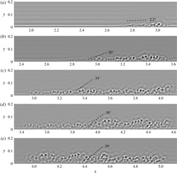
is illustrated by the spatial evolution of filtered component fields with
 ${\mathcal{L}}_{j}=35\unicode[STIX]{x1D6FF}_{\unicode[STIX]{x1D708}}$
for
 $Ma_{\infty }=2.25$
in figure 10, where various
 $x=x_{c}$
are selected from the laminar state to the turbulent state, and
 $\langle \unicode[STIX]{x1D6FC}\rangle$
at scale 8 in figure 9(a) is marked by dashed lines in figure 10. In figure 10(a), the small-scale structures with small
 $\langle \unicode[STIX]{x1D6FC}\rangle$
appear in the laminar region. Then the small-scale structures are lifted in the transitional region in figure 10(b–d), and finally converged in the turbulent region in figure 10(e).
Evolution of the filtered component fields at scale 8 with
 ${\mathcal{L}}_{j}/\unicode[STIX]{x1D6FF}=0.0397$
on the
 $x$
–
 $y$
plane in the transitional region at
 $Ma_{\infty }=2.25$
. Averaged inclination angles are sketched in dashed lines. (a)
 $x_{c}=2.5$
, (b)
 $x_{c}=3$
, (c)
 $x_{c}=3.5$
, (d)
 $x_{c}=4$
, (e)
 $x_{c}=4.5$
.

4 Image-based modelling of the skin-friction coefficient
4.1 Model equation
It is inspiring that the rapid growth of the averaged inclination angle in scalar images coincides with the increasing trend of the skin-friction coefficient in the boundary-layer transition. Next, we seek a quantitative connection between
 $\langle \unicode[STIX]{x1D6FC}(x,{\mathcal{L}}_{j})\rangle$
and
 $c_{f}(x)$
.
From the inclination-angle statistics of the filtered component fields on the
 $x$
–
 $y$
plane at different scales, we propose a simple image-based model of the skin-friction coefficient by blending
 $c_{fL}$
in (2.11) and
 $c_{fT}$
in (2.13) as
 $$\begin{eqnarray}c_{f,model}(x)=(1-\unicode[STIX]{x1D6FE}_{\unicode[STIX]{x1D6FC}})\,c_{fL}(x_{L})+\unicode[STIX]{x1D6FE}_{\unicode[STIX]{x1D6FC}}\,c_{fT}(x_{T}),\end{eqnarray}$$
with
 $$\begin{eqnarray}\unicode[STIX]{x1D6FE}_{\unicode[STIX]{x1D6FC}}(x)=\left(\frac{\langle \unicode[STIX]{x1D6FC}(x,{\mathcal{L}}_{j})\rangle -\overline{\langle \unicode[STIX]{x1D6FC}(x,{\mathcal{L}}_{j})\rangle |L_{x1}\leqslant x\leqslant x_{L}}}{\overline{\langle \unicode[STIX]{x1D6FC}(x,{\mathcal{L}}_{j})\rangle |x_{T}\leqslant x\leqslant L_{x2}}-\overline{\langle \unicode[STIX]{x1D6FC}(x,{\mathcal{L}}_{j})\rangle |L_{x1}\leqslant x\leqslant x_{L}}}\right)^{\unicode[STIX]{x1D709}}.\end{eqnarray}$$
Here the subscript ‘
 $L$
’ denotes the quantities in the laminar region, and ‘
 $T$
’ the quantities in the fully developed turbulent region;
 $x_{L}$
and
 $x_{T}$
denote the reference locations of laminar and fully developed turbulent regions, respectively;
 $\overline{\langle \unicode[STIX]{x1D6FC}\rangle |L_{x1}\leqslant x\leqslant x_{L}}$
and
 $\overline{\langle \unicode[STIX]{x1D6FC}\rangle |x_{T}\leqslant x\leqslant L_{x2}}$
denote conditional averages of
 $\langle \unicode[STIX]{x1D6FC}\rangle$
over laminar and turbulent regions, respectively, for normalizing
 $\langle \unicode[STIX]{x1D6FC}\rangle$
in (4.2).
Figure 9 shows that the averaged inclination angle is close to
 $0^{\circ }$
at
 $x=x_{L}$
in the laminar state, then it increases sharply in the transitional region and finally it converges to a statistically steady value around
 $x=x_{T}$
in the fully developed turbulent state. The reference locations
 $x_{L}$
and
 $x_{T}$
are searched from the rightmost and leftmost of profiles of
 $\langle \unicode[STIX]{x1D6FC}(x,{\mathcal{L}}_{j})\rangle$
by criteria
 $$\begin{eqnarray}\langle \unicode[STIX]{x1D6FC}(x_{L},{\mathcal{L}}_{j})\rangle =(\langle \unicode[STIX]{x1D6FC}(x,{\mathcal{L}}_{j})\rangle _{max}-\langle \unicode[STIX]{x1D6FC}(x,{\mathcal{L}}_{j})\rangle _{min})\times 1\,\%+\langle \unicode[STIX]{x1D6FC}(x,{\mathcal{L}}_{j})\rangle _{min},\end{eqnarray}$$
and
 $$\begin{eqnarray}\langle \unicode[STIX]{x1D6FC}(x_{T},{\mathcal{L}}_{j})\rangle =(\langle \unicode[STIX]{x1D6FC}(x,{\mathcal{L}}_{j})\rangle _{max}-\langle \unicode[STIX]{x1D6FC}(x,{\mathcal{L}}_{j})\rangle _{min})\times 99\,\%+\langle \unicode[STIX]{x1D6FC}(x,{\mathcal{L}}_{j})\rangle _{min},\end{eqnarray}$$
respectively. Here,
 $\langle \unicode[STIX]{x1D6FC}\rangle _{min}$
and
 $\langle \unicode[STIX]{x1D6FC}\rangle _{max}$
are the minimum and maximum of
 $\langle \unicode[STIX]{x1D6FC}(x,{\mathcal{L}}_{j})\rangle$
, respectively, in the subdomain of interest for
 $\unicode[STIX]{x1D719}$
.
The modelled
 $c_{f}$
is bounded by the empirical formulae (2.11) for
 $c_{fL}$
and (2.13) for
 $c_{fT}$
in (4.1), and the transition from
 $c_{fL}$
to
 $c_{fT}$
depends on
 $\unicode[STIX]{x1D6FE}_{\unicode[STIX]{x1D6FC}}$
generally ranging from 0 to 1. The imaged-based model is reminiscent of the intermittency-based model of Dhawan & Narasimha (Reference Dhawan and Narasimha1958), and
 $\unicode[STIX]{x1D6FE}_{\unicode[STIX]{x1D6FC}}$
in terms of the normalized averaged inclination angle in (4.1) can be considered as an ‘intermittency factor’ to characterize the emergence of coherent structures or the ‘turbulent spot’. The exponent in (4.2) is generally related to the steepness of the transition from
 $c_{fL}$
to
 $c_{fT}$
, and it is set to be
 $\unicode[STIX]{x1D709}=1$
unless a variable
 $\unicode[STIX]{x1D709}$
is explicitly specified. In appendix B, we demonstrate that the optimal
 $\unicode[STIX]{x1D709}=\unicode[STIX]{x1D709}({\mathcal{L}}_{j})$
is scale dependent.
4.2 Model validation
The model (4.1) of
 $c_{f}$
based on averaged inclination angles at different length scales is assessed by the relative error
 $$\begin{eqnarray}\unicode[STIX]{x1D700}_{r}=\frac{\displaystyle \int _{L}|c_{f,model}-c_{f,DNS}|\,\text{d}x/L}{\displaystyle \int _{L}c_{f,DNS}\,\text{d}x/L}\times 100\,\%,\end{eqnarray}$$
with the integral length
 $L=L_{x2}-L_{x1}$
. The relative errors for DNS at two
 $Ma_{\infty }$
are shown in figure 11. In general, the discrepancy between the model prediction
 $c_{f,model}$
and the DNS result
 $c_{f,DNS}$
decreases with decreasing the characteristic length scale in the scalar image; we achieve overall good predictions of
 $c_{f}$
with
 $\unicode[STIX]{x1D700}_{r}<15\,\%$
at intermediate and small scales as
 $0.1\unicode[STIX]{x1D6FF}$
or
 ${\mathcal{L}}_{j}<100\unicode[STIX]{x1D6FF}_{\unicode[STIX]{x1D708}}$
. Therefore, we suggest using
 $c_{f,model}$
at
 ${\mathcal{L}}_{j}\leqslant O(0.1\unicode[STIX]{x1D6FF})$
for the model prediction from experimental images of boundary-layer transition (see appendix A).
As discussed in appendix B, the model prediction can be further improved by using scale-dependent
 $\unicode[STIX]{x1D709}=\unicode[STIX]{x1D709}({\mathcal{L}}_{j})$
instead of
 $\unicode[STIX]{x1D709}=1$
in (4.2). Moreover, the intermittency factor in (4.1) and (4.2) can be modelled by the form suggested by Dhawan & Narasimha (Reference Dhawan and Narasimha1958), which is discussed in appendix C.
The relative error of
 $c_{f,model}$
calculated from the model (4.1) based on
 $\langle \unicode[STIX]{x1D6FC}(x,{\mathcal{L}}_{j})\rangle$
at various scales in terms of (a)
 ${\mathcal{L}}_{j}/\unicode[STIX]{x1D6FF}_{\unicode[STIX]{x1D708}}$
and (b)
 ${\mathcal{L}}_{j}/\unicode[STIX]{x1D6FF}$
.

Based on the error analysis, for example, we use the values of
 $\langle \unicode[STIX]{x1D6FC}\rangle$
at the length scale
 ${\mathcal{L}}_{j}\approx 0.08\unicode[STIX]{x1D6FF}$
in the model equation (4.1). As shown in figure 12, the trend of the increasing averaged inclination angle is qualitatively similar to the rise of
 $c_{f}$
, and the modelled
 $c_{f}$
in equation (4.1) agrees well with DNS results for both Mach numbers. This implies that it is possible to quantify
 $c_{f}$
, which is hard to measure in high-
 $Ma$
boundary-layer transition, from two-dimensional scalar images that are relatively easy to obtain from experimental visualization. In addition, the slight overshoot of
 $c_{f}$
at the end of the transitional region in DNS is not observed in most of the profiles of
 $\langle \unicode[STIX]{x1D6FC}\rangle$
in figure 9, resulting in the under-prediction of
 $c_{f}$
from (4.1).
Comparison of the skin-friction coefficients from DNS and the model (4.1) with
 ${\mathcal{L}}_{j}\approx 0.08\unicode[STIX]{x1D6FF}$
or
 $O(10)\unicode[STIX]{x1D6FF}_{\unicode[STIX]{x1D708}}$
, along with the averaged inclination angle of scalar structures. (a)
 $Ma_{\infty }=2.25$
, (b)
 $Ma_{\infty }=6$
.

For the further application of the image-based model in experiments, the scalar field for experimental visualization generally has a finite diffusivity instead of the vanishing diffusivity in the Lagrangian field in the present DNS, so the real scalar field has a finite smallest scale
 $\unicode[STIX]{x1D6FF}_{\unicode[STIX]{x1D719}}$
. Since the effect of the diffusivity on the scalar field is similar to filtering, the discrepancy assessment of the Lagrangian field in figure 11 can be still useful for
 ${\mathcal{L}}_{j}>\unicode[STIX]{x1D6FF}_{\unicode[STIX]{x1D719}}$
if the image-based model is applied to other scalar images from experiments. In appendix A, we demonstrate that the image-based modelling of
 $c_{f}$
is applicable to experimental images in compressible boundary-layer transition.
4.3 Inclined structures and drag production
The relatively accurate prediction of
 $c_{f}$
in the image-based model indicates that the generation of inclined small-scale flow structures is closely related to the drag production. As sketched in figure 13, one possible reason is that the lifts of material surfaces during the transition, which are good surrogates of vortex surfaces consisting of vortex lines, can generate strong inclined shear layers (see Zhao et al.
Reference Zhao, Yang and Chen2016, Reference Zhao, Xiong, Yang and Chen2018) to increase
 $c_{f}$
.
Diagram of the geometry of material surfaces and typical vortex lines near the surfaces, along with the rise of
 $c_{f}$
. Solid lines denote vortex lines, and solid vectors
 $\boldsymbol{n}_{\unicode[STIX]{x1D719}}$
denote the normal of material surfaces.

Assume the flow field is filled with wall-parallel material surfaces in the laminar state with all the surface normal
 $\boldsymbol{n}_{\unicode[STIX]{x1D719}}\equiv \unicode[STIX]{x1D735}\unicode[STIX]{x1D719}/|\unicode[STIX]{x1D735}\unicode[STIX]{x1D719}|$
pointing to the wall-normal direction. In the transitional region, the near-wall material surfaces are lifted due to the growing streamwise vorticity. This elevation event is quantified by the wall-normal Lagrangian displacement
 $$\begin{eqnarray}\unicode[STIX]{x0394}Y(\boldsymbol{x}_{0},t_{0}|t)=Y(\boldsymbol{x}_{0},t_{0}|t)-y(\boldsymbol{x}_{0},t_{0}),\end{eqnarray}$$
where
 $Y$
is the wall-normal location of a fluid particle on a material surface. The displacement
 $\unicode[STIX]{x0394}Y$
quantifies the scalar transport in the wall-normal direction within a time interval of interest, and Zhao et al. (Reference Zhao, Yang and Chen2016) define the Lagrangian events ‘elevation’ with
 $\unicode[STIX]{x0394}Y>0$
and ‘descent’ with
 $\unicode[STIX]{x0394}Y<0$
. The contour of
 $\unicode[STIX]{x0394}Y$
and the contour lines of high shear
 $\unicode[STIX]{x2202}u/\unicode[STIX]{x2202}y$
in the transitional region are shown in figure 14. In general, the inclined high shear layers cover the region with
 $\unicode[STIX]{x0394}Y>0$
, which is similar to the observation in an incompressible temporal transitional channel flow in Zhao et al. (Reference Zhao, Yang and Chen2016), because the strong shear layer can be generated between the elevated low-speed fluid and the surrounding high-speed fluid. Furthermore, the region with
 $\unicode[STIX]{x0394}Y>0$
, which also corresponds to the inclined scalar structure with
 $\boldsymbol{n}_{\unicode[STIX]{x1D719}}$
, deviates from the wall-normal direction as sketched in figure 13, which can be characterized as a finite
 $\langle \unicode[STIX]{x1D6FC}\rangle$
in the multi-directional analysis. Thus the inclined high shear layers accelerate the momentum transport and produce the large Reynolds shear stress (see Zhao et al.
Reference Zhao, Yang and Chen2016), which can increase
 $c_{f}$
implied by the relation between the Reynolds shear stress and
 $c_{f}$
(see Fukagata et al.
Reference Fukagata, Iwamoto and Kasagi2002; Gomez, Flutet & Sagaut Reference Gomez, Flutet and Sagaut2009).
The contour of the Lagrangian wall-normal displacement
 $\unicode[STIX]{x0394}Y$
and contour lines for the strong shear layers on the
 $x$
–
 $y$
plane in the transitional region at
 $Ma_{\infty }=6$
.

5 Conclusions
We develop a model of the skin-friction coefficient
 $c_{f}$
based on the inclination-angle statistics of small-scale scalar structures in the images on streamwise and wall-normal planes. The DNS of spatially evolving flat-plate compressible boundary layers is performed at
 $Ma_{\infty }=2.25$
and 6, and then the backward-particle-tracking method is applied to evolve the Lagrangian scalar field in the Eulerian velocity field from DNS. The multi-scale and multi-directional geometric analysis with the sliding window filter is then applied to characterize the averaged inclination angle of spatially evolving scalar structures at a range of scales from a boundary-layer thickness to several viscous length scales.
The averaged inclination angle increases along the streamwise direction, and the trend is qualitatively similar to the rise of
 $c_{f}$
. In the laminar region, the averaged inclination angle is almost
 $0^{\circ }$
, then it increases sharply in the transitional region and finally it converges to a statistically steady value in the fully developed turbulent region.
The imaged-based model blends the empirical formulae of
 $c_{f}$
in the laminar and fully developed turbulent regions using the increasing normalized averaged inclination angle of scalar structures at intermediate and small scales, where the averaged inclination angle can be considered as an intermittency factor in the streamwise direction. The modelled
 $c_{f}$
calculated from flow boundary conditions and the scalar images containing the transitional region agree well with DNS results for both Mach numbers 2.25 and 6. The minimum relative error of the model, which is less than 15 %, is achieved from small-scale scalar structures at the length scale
 ${\mathcal{L}}_{j}<100\unicode[STIX]{x1D6FF}_{\unicode[STIX]{x1D708}}$
or
 $0.1\unicode[STIX]{x1D6FF}$
. We remark that the current model is free from empirical model parameters, and we also show the potential for further improvement on the model accuracy in appendices B and C by introducing an ad hoc model parameter. Furthermore, we demonstrate the applicability of the imaged-based model of
 $c_{f}$
to experimental images in appendix A.
The good performance of the image-based model implies that it is possible to convert the qualitative knowledge of coherent structures into a predictive model of the physical quantities concerned in engineering applications. The present modelling strategy of blending the empirical formulae of
 $c_{f}$
at the two extreme states is a simple stretch transform of the averaged inclination angle, and more sophisticated, machine-learning based algorithms (see Duraisamy, Iaccarino & Xiao Reference Duraisamy, Iaccarino and Xiao2019) could be applied to a larger database of scalar images for training better models.
A natural line of extension of this work is to extend the image-based model to experimental imaging in flat-plate boundary-layer transition with various free-stream turbulence levels or to other transitional wall flows, e.g. boundary-layer transition on a concave or convex wall (e.g. Wang et al. Reference Wang, Wang and Zhao2016, Reference Wang, Wang, Sun, Yang, Zhao and Hu2019). The image-based model could be extended to predict other important flow properties such as the heat transfer and turbulent noise, which are related to the coherent structures, after appropriate adaption or modification. In addition, the model could facilitate the data assimilation with experimental and computational results to improve flow predictions.
Acknowledgements
Y.Y. thanks Y. Zhao, X. Li and H. Xiao for helpful comments, and S. Yi, Y.-X. Zhao and R. Lin for the discussion of experimental NPLS imaging. Numerical simulations were carried out on the TH-2A supercomputer in Guangzhou, China. This work has been supported in part by the National Natural Science Foundation of China (nos. 11522215, 91541204 and 91841302).
Appendix A. Modelling of
 $c_{f}$
from experimental images

In this section, we demonstrate the applicability of the image-based modelling of
 $c_{f}$
for the experiment of a flat-plate supersonic boundary-layer transition. The modelling procedure, including the extraction of sliding window filter, multi-scale, multi-directional analysis and the modelling equation of
 $c_{f}$
, is the same as that for DNS. We remark that compared with the Lagrangian scalar in DNS, the experimental images of scalar structures suffer from background noise and an insufficient resolution of the smallest flow and scalar scales.
The experiment was performed in the KD-03 supersonic wind tunnel with the low free-stream turbulence level 0.4 % at the National University of Defense Technology by He et al. (Reference He, Yi, Zhao, Tian and Chen2011b
), and the NPLS experimental system is sketched in figure 15. In the test section of
 $120\times 100~\text{mm}^{2}$
, a horizontal flat plate was placed 30 mm above the floor. Experimental parameters are given in table 6, where
 $T_{0}$
,
 $P_{0}$
,
 $T_{s}$
and
 $P_{s}$
denote the total temperature, total pressure, static temperature and static pressure, respectively. Experimental images were obtained in streamwise–wall-normal (
 $x$
–
 $y$
) planes. The laser sheet is normal to the wall along the centrelines of the plate, and a charge-coupled device (CCD) camera was set normal to the laser sheet.
A sketch of the NPLS experimental system for visualizing flow structures in the flat-plate boundary-layer transition.

Parameters in the experiment of the flat-plate boundary-layer transition in He et al. (Reference He, Yi, Zhao, Tian and Chen2011b ).

The flow structures during the transition in the images were visualized using the NPLS technique based on Rayleigh scattering (see Tian et al.
Reference Tian, Yi, Zhao, He and Cheng2009). The images of tracer nanoparticles illuminated by a pulse planar laser were recorded by the CCD camera with a resolution
 $2000\times 2000$
pixels and 4096 grey scale grades. A Q-switched Nd:YAG laser was used as the light source. The pulse energy output to the test section is 350 mJ for a pulse width of 6 ns and wavelength of 532 nm. The laser beam is oriented by an articulated arm and focused as a uniform sheet by a cylindrical lens. Ten NPLS images were sampled at different times. The sampling time interval 0.2 s is much larger than a flow-through time, the ratio of the flat-plate length to
 $U_{\infty }$
in the experiment, so they can be considered as independent samples for further statistical study. The resolution of each original image is
 $1856\times 211$
pixels within the region of
 $x\in [10,32]$
cm and
 $y\in [0,2.5]$
cm, where the origin of coordinates is at the intersection of the leading edge and plate centreline. In the implementation, the region remote from wall and without coherent structures at
 $y>0.5$
cm is removed in the images for preventing the interference of image background noises on the multi-scale diagnostics.
A typical NPLS image on the
 $x$
–
 $y$
plane is shown in figure 16. The grey scale of the NPLS image is normalized from 0 to 1 and it is proportional to the particle number-density field and to the local density in the laminar region (see Tian et al.
Reference Tian, Yi, Zhao, He and Cheng2009), so the transition from dark (low grey scale) to light along the
 $y$
-direction represents the variation of
 $\unicode[STIX]{x1D70C}$
from low to high. In the upstream region, the laminar boundary layer grows linearly, and wave-like structures appear further downstream and the flow becomes unstable. In the downstream region, the breakdown of large-scale structures’ signals the transition from laminar to turbulent flow. The flow-following ability of the nanoparticles in NPLS has been validated in various experiments of supersonic flows (e.g. Tian et al.
Reference Tian, Yi, Zhao, He and Cheng2009; He et al.
Reference He, Yi, Zhao, Tian and Chen2011b
; Wang et al.
Reference Wang, Wang and Zhao2016). Therefore, the grey scale in the NPLS image for visualizing flow structures is very similar to the Lagrangian scalar in figure 7 from DNS. Here we use the same symbol
 $\unicode[STIX]{x1D719}$
to denote the grey scale of images as a NPLS scalar field.
The grey scale of a NPLS image of the flat-plate supersonic turbulent boundary-layer flow at
 $Ma_{\infty }=3$
.

For each NPLS image, we apply the sliding window filter to extract the instantaneous filtered component fields
 $\unicode[STIX]{x1D719}_{f}(x,t)$
at a sequence of window centres
 $x=x_{c}$
with the marching interval
 $\unicode[STIX]{x0394}x_{c}=1.5$
cm and the fixed cutoff window width
 $l_{c}=3$
cm from the entire NPLS field
 $\unicode[STIX]{x1D719}$
. Then
 $\unicode[STIX]{x1D719}_{f}(x,t)$
is decomposed into various scales. Figure 17 depicts the multi-scale decomposition of a typical
 $\unicode[STIX]{x1D719}_{f}$
at
 $x\in [22,25]$
cm in the transitional region. We observe that the averaged inclination angle increases with the decreasing length scale, consistent with the observation in figure 8 from DNS. The normalized characteristic scales for each scale index
 $j$
are quantified in table 7, where the characteristic length scale in the NPLS image is
 ${\mathcal{L}}_{j}=2^{-j}$
cm, the boundary-layer thickness is estimated as
 $\unicode[STIX]{x1D6FF}=0.5$
cm in the turbulent region and the viscous length scale
 $\unicode[STIX]{x1D6FF}_{\unicode[STIX]{x1D708}}=2.49~\unicode[STIX]{x03BC}\text{m}$
is calculated from the averaged
 $c_{fT}$
in (2.13) over the turbulent region.
Characteristic length scales
 ${\mathcal{L}}_{j}=2^{-j}$
cm normalized by the boundary-layer thickness
 $\unicode[STIX]{x1D6FF}=0.5$
cm or the viscous length scale
 $\unicode[STIX]{x1D6FF}_{\unicode[STIX]{x1D708}}=2.49~\unicode[STIX]{x03BC}\text{m}$
.

Scale decomposition of the NPLS scalar field on the
 $x$
–
 $y$
plane in a transitional boundary layer at
 $Ma_{\infty }=3$
and
 $x_{c}=23.5$
cm. Averaged inclination angles are sketched by dashed lines. (a) Original field, (b) filtered component field at scale 4 with
 ${\mathcal{L}}_{j}/\unicode[STIX]{x1D6FF}=0.125$
, (c) scale 5 with
 ${\mathcal{L}}_{j}/\unicode[STIX]{x1D6FF}=0.0625$
, (d) scale 6 with
 ${\mathcal{L}}_{j}/\unicode[STIX]{x1D6FF}=0.0313$
.

The averaged inclination angle
 $\langle \unicode[STIX]{x1D6FC}(x,{\mathcal{L}}_{j})\rangle$
of the NPLS scalar field in a sliding window is calculated from
 $\unicode[STIX]{x1D719}_{f}$
at each
 ${\mathcal{L}}_{j}$
using the multi-directional decomposition and averaged over 10 sample images. In figure 18(a),
 $\langle \unicode[STIX]{x1D6FC}(x,{\mathcal{L}}_{j})\rangle$
generally grows with
 $x$
and with the decreasing
 ${\mathcal{L}}_{j}$
at the same
 $x=x_{c}$
, which is consistent with the observation in figure 17 and the results in figure 9 from DNS. In addition,
 $\langle \unicode[STIX]{x1D6FC}\rangle$
for large scales
 $j=1$
and 2 are very close to zero and have little variation (not shown). For very small-scale structures, as shown in figures 17(d), the NPLS image is contaminated by the background noise, as the grain-like structures remote from the wall. Note if an image is very noisy, e.g. as a delta-correlated scalar field,
 $\langle \unicode[STIX]{x1D6FC}\rangle$
calculated from (2.22) in the multi-directional decomposition is approximately
 $45^{\circ }$
. Therefore,
 $\langle \unicode[STIX]{x1D6FC}\rangle$
for small scales
 $j=7\sim 9$
gradually approaches to
 $45^{\circ }$
owing to the background image noise.
Modelling of
 $c_{f}$
based on experimental images of the boundary-layer transition at
 $Ma_{\infty }=3$
. (a) Evolution of the averaged inclination angle (degrees) for various filtered component fields. (b) The skin-friction coefficients calculated from the model (4.1) based on
 $\langle \unicode[STIX]{x1D6FC}(x,{\mathcal{L}}_{j})\rangle$
at different scales.

Based on
 $\langle \unicode[STIX]{x1D6FC}(x,{\mathcal{L}}_{j})\rangle$
calculated from experimental images at intermediate scales, we apply the model (4.1) to estimate the skin-friction coefficient, where
 $c_{fL}$
and
 $c_{fT}$
are calculated from (2.11) and (2.13), respectively, with the parameters listed in table 6. In figure 18(b), the modelled
 $c_{f}$
satisfies the empirical formulae in laminar and fully developed turbulent regions, and provides reasonable and consistent estimations in the transitional region roughly from 20 to 25 cm. As mentioned in the introduction, the accurate measurement of
 $c_{f}$
in the experiment of supersonic wall flows is very challenging, so we can only validate that the modelled
 $c_{f}$
at least qualitatively captures the transition from
 $c_{fL}$
to
 $c_{fT}$
based on the characteristic orientation statistics at intermediate and small scales in experimental images.
Moreover, Zheng et al. (Reference Zheng, Yang and Chen2016) showed that the evolution of the averaged sweep angle defined on
 $x$
–
 $z$
planes decays almost monotonically along the streamwise direction in compressible boundary-layer transition. Thus the modelled intermittency factor (4.2) can be extended to depending on the averaged sweep angle, so that the experimental images on wall-parallel planes can also be used in the modelling of
 $c_{f}$
.
Appendix B. Optimal
$\unicode[STIX]{x1D709}$
in the modelled intermittency factor

In the model (4.1) of
 $c_{f}$
, the normalized averaged inclination angle of the filtered component fields can be considered as a surrogate of the intermittency factor in Dhawan & Narasimha (Reference Dhawan and Narasimha1958), but its profile depends on the filtering scale in figure 9, particularly at large scales. In order to mitigate the scale dependence and achieve more accurate prediction of
 $c_{f}$
, the optimal scale-dependent exponent
 $\unicode[STIX]{x1D709}=\unicode[STIX]{x1D709}({\mathcal{L}}_{j})$
in (4.2), instead of the default value
 $\unicode[STIX]{x1D709}=1$
, is considered and calculated by a searching algorithm that minimizes
 $\unicode[STIX]{x1D700}_{r}$
by varying
 $\unicode[STIX]{x1D709}({\mathcal{L}}_{j})$
for each scale. We find that
 $\unicode[STIX]{x1D709}({\mathcal{L}}_{j})$
generally decays with
 ${\mathcal{L}}_{j}$
in figure 20. By comparing figures 11 and 19, the relative errors for the scale-dependent
 $\unicode[STIX]{x1D709}({\mathcal{L}}_{j})$
, which are less than 10 % with
 ${\mathcal{L}}_{j}<0.1\unicode[STIX]{x1D6FF}$
or
 ${\mathcal{L}}_{j}<50\unicode[STIX]{x1D6FF}_{\unicode[STIX]{x1D708}}$
, are much smaller than those for
 $\unicode[STIX]{x1D709}=1$
.
The relative error of
 $c_{f,model}$
calculated from the model (4.1) based on
 $\langle \unicode[STIX]{x1D6FC}(x,{\mathcal{L}}_{j})\rangle$
at different scales with
 $\unicode[STIX]{x1D709}=\unicode[STIX]{x1D709}({\mathcal{L}}_{j})$
.

The skin-friction coefficients calculated from the image-based model (4.1) with the optimal
 $\unicode[STIX]{x1D709}({\mathcal{L}}_{j})$
at different scales are compared to
 $c_{f}$
from DNS in figure 21. In general, the predicted profiles of
 $c_{f}$
based on the optimal
 $\unicode[STIX]{x1D709}({\mathcal{L}}_{j})$
collapse with small discrepancies for intermediate and small scales.
The optimal scale-dependent exponent
 $\unicode[STIX]{x1D709}({\mathcal{L}}_{j})$
at different scales.

Comparison of the skin-friction coefficients from DNS and the model (4.1) with
 $\unicode[STIX]{x1D709}({\mathcal{L}}_{j})$
at different scales. (a)
 $Ma_{\infty }=2.25$
, (b)
 $Ma_{\infty }=6$
.

However,
 $\unicode[STIX]{x1D709}({\mathcal{L}}_{j})$
is determined by DNS results and varies with different Mach numbers in figure 20. Thus although this ad hoc model parameter can further improve the model prediction of (4.1), it is challenging to directly apply without a priori information of
 $\unicode[STIX]{x1D709}({\mathcal{L}}_{j})$
for other flows. We expect to investigate whether there exists a universal form of
 $\unicode[STIX]{x1D709}({\mathcal{L}}_{j})$
in future work.
Appendix C. Image-based modelling of
$c_{f}$
with the intermittency factor of Dhawan and Narasimha

In this section, we provide another option to estimate the intermittency factor in the image-based model of
 $c_{f}$
. Dhawan & Narasimha (Reference Dhawan and Narasimha1958) suggested a half-Gaussian shape for the intermittency factor. Based on the profile of the averaged inclination angle in scalar images, the intermittency factor in the function shape suggested by Dhawan & Narasimha (Reference Dhawan and Narasimha1958) can be determined by
 $$\begin{eqnarray}\unicode[STIX]{x1D6FE}_{DN}=\left\{\begin{array}{@{}ll@{}}\displaystyle 1-\exp \left[-\frac{(x-x_{L})^{2}}{l_{tr}^{2}}\right], & x\geqslant x_{L},\\ 0, & x<x_{L}.\end{array}\right.\end{eqnarray}$$
Here,
 $l_{tr}=(x_{T}-x_{L})/\unicode[STIX]{x1D70E}_{tr}$
is a measure of the extent of the transitional region, where
 $x_{L}$
and
 $x_{T}$
are calculated by (4.3) and (4.4), respectively, and an empirical model parameter
 $\unicode[STIX]{x1D70E}_{tr}$
controls the width of transition in
 $\unicode[STIX]{x1D6FE}_{DN}$
.
Based on
 $\unicode[STIX]{x1D6FE}_{DN}$
, the image-based model of
 $c_{f}$
becomes
 $$\begin{eqnarray}c_{f,model}(x)=(1-\unicode[STIX]{x1D6FE}_{DN})\,c_{fL}(x_{L})+\unicode[STIX]{x1D6FE}_{DN}\,c_{fT}(x_{T}).\end{eqnarray}$$
Compared with
 $\unicode[STIX]{x1D6FE}_{\unicode[STIX]{x1D6FC}}$
implied in figure 9,
 $\unicode[STIX]{x1D6FE}_{DN}$
increases monotonically along
 $x$
and is shown to be universal in terms of the normalized streamwise coordinate in the transitional region (see Dhawan & Narasimha Reference Dhawan and Narasimha1958). The relative errors from the estimation of (C 2) with various
 $\unicode[STIX]{x1D70E}_{tr}=2$
, 2.5 and 3 for DNS at two
 $Ma_{\infty }$
are shown in figure 22, and the comparison between DNS and the model (C 2) with
 $\unicode[STIX]{x1D70E}_{tr}=2.5$
and various scales is shown in figure 23. We observe that the discrepancies are generally small and most of them are less than 15 %. For
 $\langle \unicode[STIX]{x1D6FC}(x,{\mathcal{L}}_{j})\rangle$
at large scales, estimations of
 $c_{f}$
with
 $\unicode[STIX]{x1D6FE}_{DN}$
are even better than those with
 $\unicode[STIX]{x1D6FE}_{\unicode[STIX]{x1D6FC}}$
in figure 11. On the other hand, the weakness of (C 2) is that it involves an ad hoc model parameter
 $\unicode[STIX]{x1D70E}_{tr}$
. The optimal value of
 $\unicode[STIX]{x1D70E}_{tr}$
appears to be around 2 and 3 from our modelling tests.
The relative error of
 $c_{f,model}$
calculated from the model (C 2) with various
 $\unicode[STIX]{x1D70E}_{tr}$
based on
 $\langle \unicode[STIX]{x1D6FC}(x,{\mathcal{L}}_{j})\rangle$
at different scales.

Comparison of the skin-friction coefficients from DNS and the image-based model (C 2) with
 $\unicode[STIX]{x1D70E}_{tr}=2.5$
at different scales. (a)
 $Ma_{\infty }=2.25$
, (b)
 $Ma_{\infty }=6$
.