1. INTRODUCTION
Let (X,Y) be the lifetime variables of interest with joint survival function Fo(x,y) = Pr(X > x,Y > y) and marginal survival functions Fjo(·), j = 1,2. Let F(x,y) denote the corresponding joint cumulative distribution function (c.d.f.) with marginal distributions Fj(·), j = 1,2. Assume that F1 and F2 are continuous. By the Sklar (1959) theorem, there exists a unique copula function Cd such that

where the copula function Cd(·,·) is itself a bivariate c.d.f. on [0,1]2, which captures all the scale-invariant dependence between X and Y. It follows from (1) that the representation

holds where Co(u,v) ≡ u + v − 1 + Cd(1 − u,1 − v) is itself a copula function,1
As suggested by a referee, we emphasize here that the function Co in (2) is not a survival function and, likewise, the function Cα in representation (1) of Wang and Wells (2000) is a joint c.d.f., but not a survival function.
This decomposition of the joint distribution (survival) function leads naturally to a class of semiparametric bivariate distribution (survival) functions in which the marginal distribution (survival) functions are unspecified, but the copula function is parameterized as Co(u,v) = C(u,v;αo) for some parametric copula function C(u,v;α) and some unknown parameter αo. Commonly used parametric copulas include the Gaussian copula, Student's t copula, and the Clayton, Frank, and Gumbel copulas; see Joe (1997) and Nelsen (1999) for properties of many parametric copulas.
Given the existence of a large number of parametric copulas, this class of semiparametric bivariate distribution (survival) functions is able to model many different types of dependence, allowing for any type of marginal behaviors. It has proved useful in diverse fields. Specific applications include those in finance and insurance (e.g., Frees and Valdez, 1998; Embrechts, McNeil, and Straumann, 2002); in survival analysis (e.g., Clayton, 1978; Joe, 1997; Nelsen, 1999; Oakes, 1982, 1989); in econometrics (e.g., Lee, 1983; Heckman and Honoré, 1989; Granger, Teräsvirta, and Patton, 2006; Patton, 2004, 2006; Hu, 2006), to name only a few.
Because the parametric copula function C(u,v;αo) captures all the dependence between X and Y, it is important to estimate the true but unknown copula parameter αo in any application of this class of semiparametric bivariate distribution (survival) functions. The most widely used estimator of the copula parameter αo is the two-step estimator proposed by Oakes (1994) and Genest, Quessy, and Rémillard (2006) for complete data and by Shih and Louis (1995) for censored data. In this approach, one first estimates the unknown marginal distribution (survival) functions by the rescaled empirical marginal c.d.f.s (the Kaplan–Meier estimators) and then estimates αo by maximizing the estimated log-likelihood function. Genest, Ghoudi, and Rivest (1995) and Shih and Louis (1995) establish the root-n consistency and asymptotic normality of the two-step estimator for a random sample and censored data of size n, respectively. The two-step estimator and its large-sample properties have been extended to time series settings in Chen and Fan (2006a, 2006b). Earlier papers that propose specific estimators of the copula parameter αo for specific parametric copula models include Clayton (1978), Clayton and Cuzick (1985), Oakes (1982, 1986), and Genest (1987). Except for the Gaussian copula and the independence copula, the two-step estimator of the copula parameter αo is generally inefficient; see Genest and Werker (2002). Recently, Chen, Fan, and Tsyrennikov (2006) have proposed a sieve maximum likelihood estimation (MLE) procedure for all the unknown parameters in a general semiparametric multivariate copula model. For independent and identically distributed (i.i.d.) data without censoring, they show that the sieve MLEs of αo, F1, and F2 are all asymptotically efficient.
One important issue in applying this class of semiparametric distribution (survival) function models to a given data set is how to choose an appropriate parametric copula. Effort has been made to resolve this issue. For complete data, Chen, Fan, and Patton (2003), Fermanian (2005), and Genest et al. (2006), among others, develop goodness-of-fit tests for the correct specification of a parametric copula. For censored data, Wang and Wells (2000) propose a goodness-of-fit test for the correct specification of a parametric Archimedean copula, extending existing results of Genest and Rivest (1993) and Barbe, Genest, Ghoudi, and Bruno (1996) for complete data. One drawback of these tests is that if the null hypothesis of correct parametric specification is rejected, they provide no guidance as to which copula model to use.
In addition to the goodness-of-fit test, Wang and Wells (2000) also propose a model selection procedure based on comparing estimates of the integrated squared difference between the true Archimedean copula and a parametric copula for different parametric Archimedean copula models; the one with the smallest value of the integrated squared difference is chosen over the rest of the models. For example, Wang and Wells (2000) fit the Clayton, Gumbel, Frank, and log-copula models to the data set in McGilchrist and Aisbett (1991) from a study of the recurrence time of infection in kidney patients using a portable dialysis machine. They find that the corresponding values (×10−4) of the integrated square difference are 21.72, 11.23, 12.44, and 16.14 and conclude that the Gumbel model provides the best fit to the data. Note that to compute the values of the integrated squared difference one needs to estimate the copula parameter associated with each of the parametric Archimedean copula models. In the preceding application, instead of estimating the copula parameter by minimizing the integrated squared difference over all possible values of the parameter, Wang and Wells (2000) estimate the copula parameter of each Archimedean copula model by inverting Kendall's tau (τ). As such, the corresponding estimates of the parametric copulas may not estimate the closest copulas from each parametric family to the true data generating process, and the values of the integrated squared difference being compared may not estimate the distance between each parametric copula family to the true copula. Moreover, because of data reuse, it is not clear if the Gumbel model provides a significantly better fit to the data than the rest of the copula models.
The purpose of this paper is twofold. First, we demonstrate that for selection among candidate copula models that might all be misspecified, estimators of the copula parameters based on minimizing the selection criterion function may be preferred to other estimators, because the former consistently estimate the copulas in each parametric family least distant to the true copula. This ensures that the copulas being compared in the selection process are indeed the closest members from each parametric family to the true copula, consistent with the statement that Wang and Wells made in their Rejoinder to the Comment of Peña on their original article: “Our specific focus on an information-based criterion leads directly to a sensible definition of a best model as the model that minimizes a distance between itself and the underlying data-generating process.” Second, we provide a formal statistical test for Archimedean copula model selection to address the issue of data reuse as raised by Peña in his comment on Wang and Wells (2000). Our test extends the reality check for data snooping of White (2000) to the semiparametric Archimedean copula model selection for censored data.
The remainder of this paper is organized as follows. Section 2 provides a brief review of dependence properties of commonly used parametric Archimedean copulas and the nonparametric method for estimating an Archimedean copula based on censored data. In Section 3, we introduce the model selection criterion used in this paper and provide a rigorous treatment of the estimation of the criterion function. In Section 4, we put copula model selection in the context of hypothesis testing and develop a test for model selection. Section 5 presents results based on a simulation experiment and two real data sets. Some concluding remarks are provided in Section 6. All the proofs are gathered in the Appendix. In what follows, we use ⇒ to denote weak convergence.
2. ARCHIMEDEAN COPULAS AND THEIR NONPARAMETRIC ESTIMATION
2.1. A Brief Review of Archimedean Copulas
A (bivariate) copula is said to be Archimedean if it can be expressed in the form

for some convex, strictly decreasing function φ(u) from [0,1] to [0,∞] satisfying φ(1) = 0. By convention, φ−1(v) is taken equal to zero whenever v ≥ φ(0). The function φ(·) is often referred to as a generator of the corresponding Archimedean copula. For a parametric Archimedean copula C(u,v;α), we use φα(u) to denote its generator. For an Archimedean copula Cφ with generator φ, its Kendall's tau (τ) is given by

and its lower and upper tail dependence parameters are (see Nelsen, 1997):


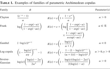
Commonly used parametric Archimedean copulas include Frank, Clayton, and Gumbel copulas. The expressions of their generators are listed in Table 1. These copulas have different dependence properties. For example, the Clayton copula exhibits positive dependence (i.e., its Kendall's τ is always positive) and lower tail dependence (λL ∈ (0,1]) but no upper tail dependence (λU = 0); as α increases, both its overall dependence (in terms of Kendall's τ) and its lower tail dependence increase. The Gumbel copula has positive dependence and upper tail dependence but no lower tail dependence; as α increases, both its overall dependence and its upper tail dependence increase. The Frank copula has symmetric positive and negative dependence but no tail dependence; as |α| increases, its overall dependence increases.
Examples of families of parametric Archimedean copulas

The class of semiparametric survival distributions with Archimedean copulas includes the commonly used frailty models in empirical studies of survival data as a subclass. This partially explains their popularity; see Joe (1997), Nelsen (1999), Clayton (1978), and Oakes (1982) for examples of applications. A bivariate frailty model for survival or lifetime variables X,Y assumes that X and Y are conditionally independent given a positive random variable W called frailty and that they satisfy

where BX(·) and BY(·) are baseline survival functions. In the numerical studies reported in Section 5 of this paper, we include two Archimedean copulas that are generated from frailty models: log-copulas corresponding to Hougaard's power variance functions (see Hougaard, 1986) and inverse-Gaussian copulas corresponding to the inverse-Gaussian frailties (see Oakes, 1989). Their generators are also listed in Table 1. As shown in Genest and Rivest (1993), the log-copulas include Gumbel and Clayton copulas as limiting cases. Namely, the log-copula with parameters α,γ converges to Gumbel copula with parameter α as γ → 0 and to the Clayton copula with parameter 1/γ as α → ∞. Using definitions (5) and (6), one can show that inverse-Gaussian copulas have neither upper nor lower tail dependence, and for α,γ ∈ (0,∞), log-copulas have no tail dependence either.
Many properties of Archimedean copulas can be found in Joe (1997) and Nelsen (1999). We end this brief review by stating an important property of Archimedean copulas that is the basis for our model selection test. Let (U,V) be uniform random variables with an Archimedean copula function Cφ(u,v). For v ∈ [0,1], define K(v) = Pr(Cφ(U,V) ≤ v), the distribution function of Cφ(U,V). Genest and Rivest (1993) show that there is a one-to-one mapping between the generator φ and

for an arbitrary constant 0 < v0 < 1 and hence a one-to-one mapping between the Archimedean copula and K. For convenience, the expressions for K corresponding to the parametric copulas used in the numerical studies in Section 5 are listed in Table 1.
2.2. Nonparametric Estimation
Let (W1,W2) be the nuisance censoring variables. With right-censored data, one observes

and a pair of indicators, (δ1,δ2) = {I(X ≤ W1),I(Y ≤ W2)}, where X ∧ W1 = min(X,W1) and I(·) is the indicator function. Suppose n i.i.d. observations

are available, where

and (δ1i,δ2i) = {I(Xi ≤ W1i),I(Yi ≤ W2i)}. Throughout the paper we assume that the true but unknown joint survival function of (X,Y) takes an Archimedean form: Fo(x,y) ≡ Co(F1o(x),F2o(y)) ≡ φo−1[φo(F1o(x)) + φo(F2o(y))], where φo(·) is a generator function of the copula Co(·,·).
Let Ko(v) ≡ Pr(Fo(X,Y) ≤ v), the distribution function of the random variable Fo(X,Y). Because there is a one-to-one mapping from the Archimedean copula Co and Ko, we will focus on the nonparametric estimation of Ko.
When complete observations on (X,Y),{(Xi,Yi)}i=1n, are available, Genest and Rivest (1993) propose estimating Ko(v) by

, where Fn(x,y) is the empirical distribution function of {(Xi,Yi)}i=1n. Barbe et al. (1996) establish the weak convergence of the process {Kn(·)} to a Gaussian process.
For censored data, Wang and Wells (2000) propose a consistent estimator of Ko(v):

where

and

are ordered observations of

and

is the estimated mass at

in which

is a nonparametric estimate of F(x,y).
For the paper to be self-contained, we restate the conditions and asymptotic properties of

established in Wang and Wells (2000).
A1. The distribution function Ko(v) admits a continuous density ko(v).
A2. Let

denote the support of

. Given Fo(x,y) = v, there exist a version of the conditional distribution of (X,Y) and a countable family

of partitions

on

into a finite number of Borel sets satisfying

, such that for all

, the mapping v → μv(A) = ko(v)Pr{(X,Y) ∈ A|Fo(X,Y) = v} is continuous.
B1.

is a uniformly and strongly consistent estimator of Fo(x,y) for

.
B2.

converges weakly to W(x,y), where W(x,y) is a continuous mean-zero Gaussian process on

, where

denotes Skorohod space.
For independent censoring, the bivariate Kaplan–Meier estimator introduced in Dabrowska (1988) satisfies B1 and B2; see Dabrowska (1989). In addition to weak convergence of the bivariate Kaplan–Meier estimator, Dabrowska (1989) also establishes the law of iterated logarithm and the validity of the bootstrap version of the bivariate Kaplan–Meier estimator. This estimator will be used in the numerical studies in this paper. The following lemma summarizes the results of Theorem 1 in Wang and Wells (2000).
LEMMA 2.1. Under B1, for 0 < ς = Fo(τ1,τ2) ≤ v ≤ 1 with

,

. Furthermore, if A1, A2, and B2 hold, then on

,

3. MODEL SELECTION AND PARAMETRIC ESTIMATION
For each j = 1,2,…, M, let

be a class of parametric Archimedean copulas. Let Kj(v;αj) ≡ Pr(Cj(F1o(X),F2o(Y);αj) ≤ v). Then, by the result of Genest and Rivest (1993), model selection of semiparametric Archimedean survival models can be based on the difference between

and Ko(v). In particular, Wang and Wells (2000) propose a copula model selection procedure using the integrated squared difference between

and Ko(v).
Define the integrated squared difference as

where ς is the smallest value of Fo(x,y) such that the estimator

consistently estimates Ko(v) for v ∈ [ς,1]; see Lemma 2.1 in Section 2.2. Define

Then Kj(v;αj*) corresponds to the copula in

closest to the true copula according to the integrated squared difference criterion, and the distance from the jth model class to the true copula is Sj(αj*) (j = 1,…, M).
For j = 1,…, M, the value αj* is referred to as the pseudo-true value, as it leads to the copula function in the jth model class that best approximates the true copula. Obviously if the copula Cj(u1,u2;αj) correctly specifies the true copula in the sense that there exists αjo such that Ko(v) = Kj(v;αjo), then αj* = αjo and Sj(αj*) = 0. In general, however, all the parametric copulas being entertained may misspecify the true copula, and the M best copulas Kj(v;αj*), one from each class

, j = 1,…, M, are compared with each other in the selection process. The class

is selected if Si(αi*) < Sj(αj*) for all j = 1,…, M and j ≠ i. In practice, neither Ko(v) nor αj* is known. Any model selection procedure will then be based on estimates of Ko(v) and αj* or equivalently of Sj(αj*), j = 1,…, M.
3.1. Estimation of αj*
The choice of an appropriate estimator of αj* is a delicate issue and deserves a rigorous treatment. When

correctly specifies the true copula model, several consistent estimators of αj* are available in the literature, including the two-step estimator of Shih and Louis (1995), the minimum distance estimator proposed in Wang and Wells (2000), and the estimator based on Kendall's τ. In Section 3.1, we study asymptotic properties of the minimum distance estimator in the general case that

misspecifies the true model, and we discuss the pros and cons of basing model selection on different parametric estimators in Section 3.2.
Let

. The minimum distance estimator is defined as

Wang and Wells (2000) establish the asymptotic properties of

when the copula class

correctly specifies the true copula of (X,Y). In this case, αj* = αjo. In general, because

and

is a consistent estimator of Ko(v) for v ∈ [ς,1], we expect

to be a consistent estimator of αj* regardless of whether

correctly specifies the true copula. The formal results are stated in the following proposition.
In what follows, Dα stands for the operator of differentiation with respect to α: Dα f (·,α) = ∂f (·,α)/∂α for a function f (·,α) depending on α.
PROPOSITION 3.1. Suppose

is a compact subset of

< with nonempty interior and αj* is the unique minimizer of Sj(αj) over

. Moreover, assume that Kj(v;αj) is twice differentiable with respect to αj with bounded derivatives. Then the following results hold.
(i)

is consistent for αj*.
(ii) Let αj* be an interior point of

. Under A1, A2, B1, and B2,

converges in distribution to Qj, where

and X(v) is defined in Lemma 2.1.
(iii)

is a consistent estimator of Sj(αj*).
(iv) If

misspecifies the true copula, then

On the other hand, if

correctly specifies the true copula, then

, where

.
Proposition 3.1 shows that in general

consistently estimates the pseudo-true value αj*, extending the consistency result of Wang and Wells (2000) for αjo when the jth model class correctly specifies the true model. Moreover

consistently estimates Sj(αj*), justifying the use of

for model selection based on minimizing Sj(αj*) over j = 1,…, M. Proposition 3.1(iv) also implies that the limiting distribution of

is the same as that of

irrespective of whether

correctly specifies the true copula model. The only difference is that when

correctly specifies the true model,

has a degenerate limiting distribution.
3.2. Which Parametric Estimator to Use?
Many estimators, including the two-step estimator of Shih and Louis (1995), share the consistency property of

for αjo when the jth model correctly specifies the true model, but may not share the consistency property for the pseudo-true value αj* in general. The reason is that unlike the true value αjo when the jth copula class correctly specifies the true copula, the pseudo-true value αj* when the jth copula class misspecifies the true copula may change if a different distance measure is used.
To be more specific, let

be a parametric estimator other than

. Examples include the estimator based on inverting Kendall's τ used in the numerical studies in Wang and Wells (2000) and the two-step estimator in Shih and Louis (1995). Most of these estimators are optimization estimators in the sense that they can be obtained by minimizing some criterion function, say,

. For example, for an Archimedean copula, the estimator based on inverting Kendall's τ can be obtained by minimizing

, because

. The two-step estimator of Shih and Louis (1995) maximizes the pseudo-likelihood function. Under regularity conditions,

, where αjL* = argminαj[plim

. For example, for the estimator based on inverting Kendall's τ,

, whereas for the two-step estimator in Shih and Louis (1995), αjL* minimizes the Kullback–Leibler information criterion. In general, αjL* differs from αj* unless

correctly specifies the true copula, in which case both αjL* and αj* equal the true value of the parameter αjo.
PROPOSITION 3.2. Suppose

is a compact subset of

with nonempty interior and Kj(v;αj) is twice differentiable with respect to αj with bounded derivatives. In addition, assume that the estimator

satisfies

and

for some

and a nondegenerate distribution QjL.
(i)

is a consistent estimator of Sj(αjL*).
(ii) If

misspecifies the true copula, then

where

.
(iii) If

correctly specifies the true copula, then

.
Given that in general αjL* ≠ αj* unless copula class

correctly specifies the true copula, Proposition 3.2 shows that

is in general an inconsistent estimator of Sj(αj*). Any model selection procedure based on

(j = 1,…, M) may thus lead to incorrect inference unless the ranking of the M models based on Sj(αjL*) is the same as that based on Sj(αj*), or at the very least, the model that minimizes Sj(αjL*) over j = 1,…, M also minimizes Sj(αj*) over j = 1,…, M. Another difference between using

and

in model selection is that the limiting distribution of

is not the same as that of

unless

correctly specifies the true model, in which case the limiting distribution is degenerate. As Wang and Wells argue in their rejoinder to the comment of Peña on their paper: “in practice, only best approximating models exist,” it is an exception rather than the rule that any simple statistical model is able to characterize the true data generating process correctly. As a result, properties of

or

when

misspecifies the true model are most relevant to model selection.
4. A MODEL SELECTION TEST
Results in the previous section suggest the use of

in model selection. Two drawbacks of basing model selection on point estimates

only are as follows. First, the limiting distribution of

depends on model j under misspecification, even though it is the same as that of

. Second, the same data are used twice in obtaining

; see Peña's discussion of both issues in his Comment on Wang and Wells (2000). A procedure for assessing the significance of the selection result is called for. In this section, we provide a formal statistical procedure to address this issue by putting copula model selection in the context of hypothesis testing along the lines of Vuong (1989) and White (2000).
To clarify the underlying idea, consider the case where only two models are being selected (M = 2). The relevant null and alternative hypotheses are

So under H0,

will be selected and under H1,

will be selected. We will construct a test for H0 based on

.
For more than two models, we will formulate the testing problem in the same way as White (2000). Let C1(u1,u2;α1) be the benchmark copula and {Cj(u1,u2;αj)}j=2M be the candidate copulas. The null and alternative hypotheses of interest are expressed as

Under H0,

will be selected, and under H1, the model minimizing Sj(αj*) over j = 2,…, M will be selected.
In contrast to goodness-of-fit tests developed in Genest and Rivest (1993) and Wang and Wells (2000), our model selection test does not require any of the parametric copulas to correctly specify the true copula under H0. In practical applications this is most likely to be the case, and the best one can do is to select the model that best approximates the true model according to some criterion such as the integrated squared difference.
Let

, where recall that

for j = 1,…, M. The following proposition provides the basis for our test.
PROPOSITION 4.1. Suppose that for j = 1,2,…, M, the copula model j satisfies the conditions of Proposition 3.1. Then jointly n1/2{Tjn − [S1(α1*) − Sj(αj*)]}j=2,…, M ⇒ (Z2,…, ZM)′, where

Moreover, let σjj denote the variance of Zj. Then σjj = 0 if and only if model j and the benchmark model 1 are generalized nested in the sense that Kj(v;αj*) = K1(v;α1*) for almost all v ∈ [0,1].
Proposition 4.1 and the continuous mapping theorem imply

Hence under the least favorable configuration (i.e., Sj(αj*) = S1(α1*) for j = 2,…, M),

. This allows us to construct a test for H0.
Let

. Suppose σjj > 0 for at least one j = 2,…, M. Then we will reject H0 if Tn > Zα, where Zα is the upper α-percentile of the distribution of maxj=2,…, M Zj. The asymptotic power properties of this test against fixed alternatives and Pitman local alternatives follow immediately from Proposition 4.1 and are summarized in the following theorem.
THEOREM 4.2. The test based on Tn is consistent against fixed alternatives of the form H1 and has nontrivial power against local alternatives satisfying

In general, the distribution of maxj=2,…, M Zj is unknown, depending on the true survival function Fo(x,y) and the pseudo-true values αj*. To circumvent this difficulty, we propose using the naive bootstrap to approximate the null distribution of Tn. Bootstrap is also used in Wang and Wells (2000) to approximate the null limiting distribution of their goodness-of-fit test. However, because in Wang and Wells (2000) the parametric copula model being tested correctly specifies the true copula under the null hypothesis, they suggest the use of a parametric bootstrap procedure based on the estimated null model

. This approach will not work in our context, as all the parametric copula models may misspecify the true copula. The naive bootstrap, on the other hand, provides a valid procedure.
Step 1. Let

be a random sample with replacement from the original data

and let

,

, and

be the bootstrapped counterparts of

,

, and

.
Step 2. Let Tjn* be the bootstrapped value of Tjn and define its recentered value as

Step 3. Repeat steps 1 and 2 for a large number of times and define the bootstrap value of Tn as Tn* = maxj=2,…, M[n1/2TjnC*].
Step 4. Use the empirical distribution function of the resulting values Tn* to approximate the null distribution of Tn.
We show in the Appendix that the preceding bootstrap works for Tn.
THEOREM 4.3. Under the conditions of Proposition 4.1,

where P*(Tn* ≤ z) is the conditional distribution of Tn* given the original sample.
5. NUMERICAL STUDIES
Following Wang and Wells (2000), we consider five Archimedean copula models: Clayton, Frank, Gumbel, log-copula, and inverse-Gaussian. Their generators and expressions for K(v) are given in Table 1 in Section 2. For the log-copula, we assume αγ = 1 as in Wang and Wells (2000). Hence, the families of Clayton and Gumbel copulas are not nested in the family of log-copulas considered in the numerical studies.
5.1. Simulation Results
The simulation design is the same as that of Wang and Wells (2000) except that we include the inverse-Gaussian copula in the experiment. In all cases, (W1,W2) are generated from Clayton copula with Kendall's τ = 0.3, and the censoring rates in both components are controlled to be between 10 and 20%. The sample size is n = 250.2
We choose a small sample size n = 250 to match that in Wang and Wells (2000). Nevertheless, we have also tried larger sample size n = 500. For the Monte Carlo studies with larger sample size, the power of our model selection test is much improved.
Fortran code is available from the authors upon request.
5.1.1. Results Based on
 .

In this section we examine performance of the model selection procedure based on the minimum value of

. For comparison purposes, we also report results based on

, where

is the estimator based on Kendall's τ used in Wang and Wells (2000).
In the simulation study we have used Clayton copula and Frank copula as the true copula, respectively. For each true copula, we calculated the percentage of times that each copula is selected based on having the minimum value

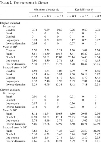
in two cases: (i) the true copula is included in the family of copula models to be selected (M = 5); (ii) the true copula is not included in the family of copula models to be selected (M = 4). As we argued earlier, case (ii) is most likely to characterize real empirical applications. As the results for Clayton and Frank copulas are very close, we report results for Clayton copula only in Table 2.
The true copula is Clayton

In addition to the percentage of times that each copula is selected, we also reported the mean and standard error of

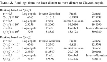
. To fully understand the results in Table 2, we provide the ranking of the remaining four copulas in terms of their distance to the true Clayton copula Sj(αj*) and their ranking based on Sj(αjL*) in Table 3, where αjL* is the probability limit of

, that is,

in which Ko(v) is the K function for Clayton copula and {Kj(v;αj)}j=14 are associated with the remaining copulas in Table 1. In all cases considered (τ = 0.3, 0.5, 0.7), the ranking of the remaining four copulas is the same regardless of whether Sj(αj*) is used or Sj(αjL*) is used. Moreover, in most of the cases, the respective values of Sj(αj*) and Sj(αjL*) are very close, although they are clearly different. Our theoretical results in Section 2 predict that the selection results based on

and

should be similar. Indeed, Table 2 provides an overwhelming amount of evidence supporting this prediction.
Rankings from the least distant to most distant to Clayton copula

Table 2 reveals that when the true Clayton copula is included, it always has the highest probability of being selected based on the minimum value criterion regardless of whether

or

is being used and the value of τ. The copula with the second highest probability of being selected is the log-copula, the closest to the true copula, although its probability of being selected is much smaller than that of the Clayton copula. In all cases except for the inverse-Gaussian with τ = 0.7, the mean and standard error of

are smaller than the mean and standard error of

. What is more important and reassuring is the fact that, based on

, when the true copula is not included, which is typically the case in empirical applications, the log-copula, being the closest to the true Clayton copula, has the highest probability of being selected and as the value of τ exceeds 0.3, the probability of selecting the log-copula reaches 1; see Table 2. Only when τ = 0.3, the probability that the log-copula is being selected decreases slightly and the inverse-Gaussian copula being the second closest to the true copula gains a small probability of being chosen. The corresponding results based on

reveal similar patterns qualitatively, although for τ = 0.3, the probability of selecting the log-copula using

is smaller than that using

. In all cases except for the inverse-Gaussian with τ = 0.7, the mean and standard error of

are smaller than the mean and standard error of

.
5.1.2. Results Based on the Model Selection Test.
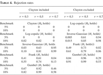
In this section, we applied the model selection test proposed in Section 4 to the same data sets generated in Section 5.1.1. When Clayton copula is included, H0 holds with Clayton being the benchmark, and H1 holds when any other copula is used as the benchmark. When Clayton copula is excluded, H0 holds with log-copula being the benchmark. The rejection rates are reported in Table 4.
Rejection rates

Table 4 indicates that the test is undersized regardless of whether the true copula is included in the selection and the true value of τ.
4As discussed in Romano and Wolf (2005), White's reality check test is asymptotically undersized unless the least favorable curve (LFC) holds. In our case, because Sj(αj*) ≠ S1(α1*), we do not have LFC and hence expect our test to be undersized. As demonstrated by Romano and Wolf (2005), Studentization may improve the size and power of the reality check test. This will be explored elsewhere.

.
5.2. Real Data Examples
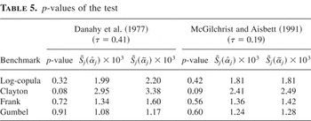
In this section, we apply our proposed model selection test to the two data sets studied in Wang and Wells (2000): the data set in Danahy, Burwell, Aranow, and Prakash (1977) and the data set in McGilchrist and Aisbett (1991). We suggest that readers consult the original papers or Wang and Wells (2000) for backgrounds on these data sets. Based on the value of

, Wang and Wells (2000) recommend the choice of Clayton or log-copula for the first data set and Gumbel for the second data set. In Table 5, we report bootstrap p-values of our model selection test, values of

and

.
p-values of the test

Based on the p-values of the test, Clayton copula is rejected for both data sets at 10% significance level and none of the other three copulas is rejected. This is consistent with the values of

; they are small for log-copula, Frank, and Gumbel compared with the value for Clayton copula. Because Clayton copula is the only one among these four copulas that has lower tail dependence, this suggests that neither data set is likely to have lower tail dependence. Based on the minimum value criterion, the Gumbel copula is selected for both data sets,
5The values of

we obtained for the first data set lead to a different ranking of the copulas from that of Wang and Wells (2000), although they lead to the same ranking as that in Wang and Wells (2000) for the second data set. They also lead to the same ranking of the copulas as

for both data sets.

for copula model selection, Table 5 indicates that p-values of the test provide an alternative model selection criterion. For both data sets, all three criteria,

,

, and the p-value, select the same copula class.
6. CONCLUSIONS
This paper makes two contributions to semiparametric survival model selection for bivariate failure-time data. First, we provide a rigorous treatment of the appropriate choice of the parametric estimator of the copula parameter in model selection. This differs from model specification testing as done in Wang and Wells (2000) because in model specification testing, under the null hypothesis, the parametric model correctly specifies the true model and hence any root-n consistent parametric estimator under the null hypothesis can be used to construct model specification tests. In model selection tests, on the other hand, there is no guarantee that any of the models being entertained correctly specifies the true model even under the null hypothesis. This makes the choice of the parametric estimator critical in model selection tests, and we recommend estimating the pseudo-true parameter by minimizing the selection criterion function. Although in this paper we address this issue in the specific context of model selection for bivariate failure-time data using the integrated squared difference criterion, it is clear that the whole idea applies to model selection tests in other contexts and to any selection criterion function. Second, we address the issue of data reuse in copula model selection pointed out by Peña in his Comment on Wang and Wells (2000) by establishing a formal statistical test for copula model selection for bivariate failure-time data.
Extension of our model selection test to multivariate failure-time data is straightforward. As the test is based on comparing Ko(v) with Kj(v;αj*), it is consistent for Archimedean copulas. For selection of multiple multivariate parametric copulas for complete data, Chen and Fan (2005) proposed pseudo-likelihood ratio tests that are consistent for any parametric copulas, including Archimedean and non-Archimedean families. Using the two-step estimator of Shih and Louis (1995) and that of Lin and Ying (1993) for various censored data, we can develop pseudo–likelihood ratio tests for general copula model selection for censored data. We are currently working on this.
APPENDIX: Technical Proofs
Proof of Proposition 3.1. Recall that

, where

. One can apply Theorems 3.4 and 6.2 in White (1994) to prove (i) and (ii).
(i) Given the conditions of Proposition 3.1, we only need to show the uniform convergence of

to Si(αi) over

in probability; see Theorem 3.4 in White (1994). This follows from consistency of

, the fact that Ko(v) and Ki(v;αi) are bounded, and the next inequality:

(ii) By Theorem 6.2 in White (1994), it suffices to show that
(a)

in distribution, and
(b)

uniformly in

.
Using the fact that Dα Si(αi*) = 0, one can easily show that

(a) follows from (A.1) and Lemma 2.1, whereas (b) follows from Lemma 2.1 and the following equation:

(iii) It is straightforward and omitted.
(iv) As in Wang and Wells (2000), we decompose

as follows:

Lemma 2.1 and Proposition 3.1(ii) imply A1 = Op(n−1), A3 = Op(n−1), and B2 = Op(n−1). By Taylor series expansion,

where αi* lies between αi* and

and the second equality follows from the fact that Dα Si(αi*) = 0 and the last from Proposition 3.1(i) and (ii). Consequently, we have

The limiting distribution of

for the case where

misspecifies the true copula follows from Lemma 2.1, the continuous mapping theorem, and (A.3). For the correct specification case, see Theorem 3 in Wang and Wells (2000). █
Proof of Proposition 3.2.
(i) is straightforward and omitted.
(ii) A similar proof to that of Proposition 3.1(iv) suggests that

The result follows from Lemma 2.1, the assumption on

, the preceding equation, and the continuous mapping theorem.
(iii) Theorem 3 in Wang and Wells (2000). █
Proof of Proposition 4.1. Equation (A.3) implies that

The conclusion follows immediately from Lemma 2.1 and the continuous mapping theorem. █
To prove Theorem 4.3, we first verify the consistency of the proposed bootstrap procedure for

and

. The results are stated in the following lemma. For compactness, we borrow the notation op*(1) pr-P and Op*(1) pr-P from Gonçalves and White (2004): Wn* = op*(1) pr-P if Wn* approaches zero in P* probability conditional on the original data and for all samples except a set of measure approaching zero, where Wn* = Op*(1) pr-P if Wn* is bounded in P* probability conditional on the original data and for all samples except a set of measure approaching zero.
LEMMA A.1. Under the conditions of Proposition 3.1,
(i) the limit process of

conditional on the original data converges to the limit process of

in probability;
(ii) the conditional distribution of

given the original data converges to the distribution of

in probability.
Proof of Theorem 4.3. It suffices to show that

Similar to the decomposition of

, we get

By Lemma A.1, we get A1* = Op*(n−1) pr-P, A3* = Op*(n−1) pr-P, and B2* = Op*(n−1) pr-P. By Taylor series expansion,

where αi* lies between

and

and the second equality follows from the fact that

and the last from Lemma A.1. Consequently, we have

The conclusion follows from Lemmas 2.1 and A.1 and Proposition 3.1. █
Proof of Lemma A.1.
(i) By Theorem 3.9.11 in Van der Vaart and Wellner (1996) and Corollary 2.2 in Dabrowska (1989), it suffices to show that the map K(F)(·):

is Hadamard differentiable at F tangentially to

, where K(F)(·) = E [I(F(X,Y) > ·)]. In fact for

, its Hadamard derivative at F is given by

Let tn → 0 and

. We need to show that

The left-hand side of (A.6) can be decomposed as follows:

Noting the similarity between An(v), Bn(v), and Cn(v) and

,

, and

, respectively, in the proof of Theorem 1 in Wang and Wells (2000), one can follow their proof to verify (A.6) by replacing weak convergence and tightness in their proof with uniform convergence and equicontinuity for the relevant functions in our case. For example, Hn plays the role of

and tn that of n−1/2 in Wang and Wells (2000).
(ii) First, we show that

pr-P. Using Lemma A.2 in Gonçalves and White (2004), it suffices to show that

pr-P. It follows from (i) of this lemma, because


Now we can apply Lemma A.3 in Gonçalves and White (2004) to show (ii). It suffices to verify conditions (b3) and (b4) of Lemma A.3 in Gonçalves and White (2004). They are
(b3) The conditional distribution of

converges to

in probability;
(b4)

pr-P.
Using the fact that

, one can show that

(b3) follows from (A.10) and (i) of this lemma. Similar to (A.2), one can show that

by part (i) of this lemma, Lemma 2.1, and boundedness of Dα2Ki(v;αi). █