

NOMENCLATURE
Acronyms and Abbreviations
- AoA
Angle-of-Attack
- C.G.
Centre of Gravity
- CFD
Computational Fluid Dynamics
- CFRP
Carbon Fibre Reinforced Polymer
- CRM
NASA Common Research Model
- DLM
Doublet-Lattice Method
- DMI
Direct Matrix Input
- FE
Finite Element
- MTOW
Maximum Take-Off Weight
- OEW
Operational Empty Weight
- PSO
Particle Swarm Optimisation
- SST
Stacking Sequence Table
- VCCTF
Variable Camber Continuous Trailing-Edge Flaps
Symbols
 $\bar{c}$
mean aerodynamic chord
- cl
sectional lift coefficient
- C
optimisation design constraints
- CL
aircraft lift coefficient
- CD
aircraft drag coefficient
- C D 0
wing zero-lift drag coefficient
- C Dc
wing wave drag coefficient
- C Dl
lift-induced drag coefficient
- C D losses
drag coefficient due to non-modelled fuselage and vertical tail
- C Dp
wing profile drag
- Cf
viscous drag coefficient
- FB
mission fuel burn
- f top − levelobj
top-level optimisation objective function
- f bottom − levelobj
bottom-level optimisation objective function
- ${\cal F}$
form factor
- h
laminate thickness
- KS
Kreisselmer-Steinhauser design constraint
- M
Mach number
- NL
number of load cases
- Np
wing patch number
- PRE
Payload-Range Efficiency parameter
- R
design mission range
- Rex
wing average Reynolds number
- S
wing planform area
- S wetted
wing wetted area
- TSFC
Thrust Specific Fuel Consumption
- t/c
thickness-to-chord ratio
- tp
wing patch thickness
- U 0
free-stream velocity
- Uk
composite material invariants, with k = 1, . . .5
- x t
optimisation design variables describing thicknesses of the main wing sub-structure components
- x comp
optimisation design variables describing in-plane and out-of-plane lamination parameters
- x jig
optimisation design variables describing the wing jig-twist shape
- x ctrl
optimisation design variables describing trailing-edge control deflections
- (x/c)max
chordwise maximum thickness position
- W
aircraft weight
- W wing
half-wing structural weight
- z
laminate through-thickness coordinate z; wing bending deformation
- θ
laminate ply angle along the through-thickness coordinate z; wing twist
- Λle
wing leading-edge sweep angle
- Λt/c max
geometric sweep angle of the maximum wing thickness line
- λmin
minimum buckling load factor
- αi
weighting factors for the bottom level optimisation objective function
- ν
kinematic viscosity
- ρKS
KS aggregation factor
- ξji
lamination parameters, with i = 1, . . .4, and j = A, D
- x
vector of design variables
- A
laminate in-plane stiffness matrix
- B
laminate bending-extension coupling stiffness matrix
- D
laminate out-of-plane stiffness matrix
- M
laminate generalised moments
- N
laminate generalised forces
- ${{{\bm \varepsilon }}^{\bf 0}}$
laminate generalised strains
- ${{\bm \kappa }}$
laminate generalised curvatures


Subscripts
- i
i th finite element; i th cruise segment, i th load case
- Lam
laminate
- MinStrain
minor principal strain
- MaxStrain
major principal strain
- MinStress
minor principal stress
- MaxStress
major principal stress
- p
wing patch number
- Stress-Mises
Von-Mises stress
- Strain-Mises
Von-Mises strain
1.0 INTRODUCTION
The current commercial aviation industry forecasts a market growth rate of approximately 5% yearly(1,2) and is facing challenging demands for improvements in fuel efficiency and greener operations (lower CO2 emissions and reduced noise pollution). This trend is further heightened by fuel prices volatilities and random market instabilities, which are becoming crucial design drivers in today's aviation industry(1). Despite the progress of conventional aircraft technologies over the past decades, fuel burn metrics are still found to be lagging behind the goals established by industry regulators(Reference Kharina and Rutherford3), indeed is well know that the industry's performance in terms of metrics such as cost per passenger mile are still improving but at a much reduced rate. It is expected that major and drastic improvements in aircraft performance are likely to be achieved only by means of potential and prospective technological enablers – for instance, the use of novel aerodynamic, propulsion and structural concepts(4) to tackle the three elements of the well-known Breguet Range Equation that can be employed to increase aircraft performance via improved lift/drag, better specific fuel consumption and less weight.
Composites are now widely used in aircraft structures with both the B787 and A350 having over 50% of their structure consisting of composite (primarily carbon fibre reinforced polymer-CFRP) materials and this increased use has been based upon their improved strength to weight characteristics compared to metals. However, virtually all applications of composite materials have failed to take account of the anisotropic characteristics of such materials and symmetric/balanced lay-ups have been used so that the composite behave as a “black-metal”. The possibilities of using composite materials to passively “tailor” the behaviour of flexible wings through coupling of the bending and torsion deflections have been known since the 1980s(Reference Shirk, Hertz and Weisshaar5) when they were applied to the forward swept wing X-29 research aircraft(Reference Weisshaar6); however, little application of aeroelastic tailoring has been applied since then to commercial airplanes.
Passive aeroelastic tailoring approaches have proven the capability to effectively minimise wingbox structural weight, for both all-metallic and composite airframes, under a variety of static and dynamic constraints(Reference Jutte and Stanford7–Reference Dillinger, Klimmek, Abdalla and Gürdal10) and to reduce fuel burn of conventional transport aircraft configurations(Reference Kennedy and Martins11–Reference Liem, Kenway and Martins15). Recent work has considered the use of novel materials and structural concepts such as tow-steering(Reference Stanford and Jutte16–Reference Stodiek, Cooper, Weaver and Kealy18) and topological optimised stiffening members(Reference Stanford and Dunning19–Reference Francois, Cooper and Weaver22), which have shown the ability to widen the design space offering additional ways to locally tailor the structure for enhanced aerostructural performance and simultaneously mitigate static and dynamic instabilities, such as panel buckling, gust loads and flutter.
It is anticipated that further significant aerostructural gains in aircraft performance will only be possible using non-conventional or hybrid design approaches, such as the so-called “integrated aeroservoelastic tailoring”(Reference Zeiler and Weisshaar23), or simply, aeroservoelastic tailoring. This discipline aims to exploit the synergies between passive aeroelastic structural adaptation and active/adaptive control of aerodynamic surfaces. The expected outcome is the creation of designs that outperform those following solely passive aeroelastic tailoring paradigms. It is worth mentioning that aeroservoelastic tailoring is used here to refer to a broader context, where the control surfaces can be used not only to improve dynamic related design qualities, but also for controlling quasi-steady aerodynamic loads at symmetric manoeuvres.
The use of control surfaces for active gusts and manoeuvre loads alleviation is well established in current transport and this reduction in loads leads to a corresponding decrease in aircraft weight and also to improve ride quality(Reference Regan and Jutte24). Moreover, a number of recent studies have explored active aeroelastic adaptations as a means to improve aircraft overall performance. It has been shown that Variable Camber Continuous Trailing-edge Flaps (VCCTF)(Reference Nguyen, Lebofsky, Ting, Kaul, Chaparro and Urnes25) can be rotated to optimal patterns for load relief (and thus achieving a lighter-weight wingbox) at symmetric and roll manoeuvres(Reference Stanford26), and/or to improve fuel burn and to mitigate flutter(Reference Stanford27,Reference Stanford28) of an all-metallic variant of the NASA Common Research Model(Reference Vassberg, DeHaan, Rivers and Wahls29) subjected to stresses, buckling, flutter and actuator constraints. There has also been interest in evaluating potential benefits of trailing-edge control devices for minimum drag(Reference Kolonay and Eastep30,Reference Duke and Weisshaar31) , particularly in cruise and in off-design conditions(Reference Lyu and Martins32,Reference Rodriguez, Aftosmis, Nemec and Anderson33) .
More recently, aeroservoelastic tailoring has been combined with spars and ribs topology optimisation to achieve more structurally efficient configurations of a composite flying-wing augmented with distributed trailing-edge flaps(Reference Zhao and Kapania34). High-fidelity aerostructural optimisations including trailing-edge shape design variables were also shown to produce solutions capable of performing aerodynamically better than a traditional design across different points in the flight envelope(Reference Burdette, Kenway and Martins35,Reference Burdette, Kenway and Martins36) . Overall, these results encourage the use of aft-camber tailoring as a prospective mechanism for improving aerodynamic efficiency at a reduced structural weight of the state-of-the-art transport aircraft.
Regardless of the growing interest in improving conventional designs using aeroservoelastic tailoring approaches, the majority of work undertaken by the research community has focused only on all-metallic solutions. No formal study that compares all-metallic and composite wingboxes augmented by trailing-edge aerodynamic devices has been made, so that potential benefits of combining composite stiffness tailoring with control surface scheduling for an aeroelastic wing remains open to question. It is thought that introducing composite materials into state-of-the-art airframes can significantly widen the design options as one can take advantage of their tailoring capabilities by concurrently designing the structure, its constituent material and control devices rotation pattern for a number of design purposes.
The goal of this paper is to perform aeroservoelastic tailoring optimisation of a transport composite wing and to understand physical behaviours that govern these configurations benchmarking the optimised solutions found with similar all-metallic counterparts. In order to do so, passive shape adaptation is combined with adaptive aft-camber tailoring of the composite wingbox with 12 distributed full-span control surfaces in order to improve fuel burn in a “cruise-climb” mission. Aeroservoelastic tailoring of the representative wingbox is sought by optimising variations in thicknesses, laminate stiffnesses, jig-twist shape and control surfaces scheduling (for both cruise drag and load relief) subjected to stresses, strains, and buckling constraints. Four different optimisation problems are carried out:
i. an all-metallic wingbox with undeflected control surfaces;
ii. a wingbox with composite skins and undeflected control surfaces;
iii. an all-metallic wingbox augmented by distributed control surfaces and;
iv. a wingbox with composite skins augmented by distributed control surfaces.
To measure the design efficiency, the optimised composite wing with trailing-edge flaps (iv) is benchmarked against an all-metallic wing obtained with the same methodology (iii). The passively tailored study cases (i) and (ii) are used as reference designs for the adaptive study cases (iii) and (iv). Performance is evaluated based on the total fuel burned and a payload-range efficiency parameter. Apart from fuel burn comparisons, special attention is drawn into investigating the interdependencies between control surface scheduling design variables and laminate stiffnesses through aerostructural load re-distribution, which, in turn, relieves the manoeuvre loads and minimises drag.
The paper is structured as follows. First, we describe the reference aircraft geometry and finite element aeroelastic model in Section 2. The aeroelastic solver used for load and stress evaluations, and additional aircraft drag considerations are briefly discussed in Section 3. Next, laminate constitutive equations and manufacturing constraints are formulated in Section 4. The optimisation problem statement is introduced formally in Section 5, with detailed descriptions of the optimisation algorithm, design variables and design constraints used. Finally, the results in terms of structural characteristics variations, spanwise loads, control surface deflections and first-order performance metrics are assessed and discussed in Section 6, followed by concluding remarks drawn in Section 7.
2.0 BASELINE LAYOUT AND GENERAL DESCRIPTION
The aircraft model used throughout this work is based on open research data provided in the development of the NASA Common Research Model (CRM)(Reference Vassberg, DeHaan, Rivers and Wahls29). The wing configuration is demonstrative of the state-of the-art of a contemporary long-range airliner (operating in the 300-seat market category) designed for nominal cruise flights at transonic speeds, more specifically, at Mach number M = 0.85 with a design lift coefficient of CL = 0.50.
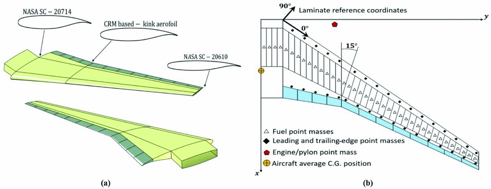
The wing planform spans 58.7m, with an aspect ratio 9 and a quarter-chord sweep angle of 35°. The trailing-edge kinks at approximately 37% of the semi-span. The mean aerodynamic chord and the taper ratio are 7.00m and 0.275, respectively. The wing root employs a NASA SC-20714 supercritical aerofoil with a maximum thickness of 14% and with 7% of maximum camber. For the outboard wing section, a NASA SC-20610 aerofoil is used. A lofted version of the CRM aerofoil developed for the 65% span station is utilised at the wing Yehudi break (kink) resulting in a maximum thickness of 12.3% with 6.3% of maximum camber. A total of 12 discrete trailing-edge controls, distributed along the wingspan as indicated in Fig. 1, are utilised as a mechanism for improved aerostructural performance. These devices occupy approximately 15% of the local wing chord.
Wing aerodynamic and structural layouts. (a) Aerodynamic shape of the reference wing model. (b) Wingbox structural configuration.

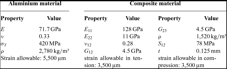
The wingbox follows a conventional structural architecture, which is built around two main full-depth straight spars (i.e. front and rear spars) with in-between ribs and stiffened skins. The front and rear spars lie respectively at 11% and 60% of the wing root chord, and taper linearly towards the wing outboard section to correspondingly 30% and 65% of the local chord. The box structure comprises three main wing partitions: wing fuselage junction (0-10%), inner wing (10-37%), and outer wing (37-100%). A total of 40 ribs is used, uniformly distributed piecewise within each of the three wing partitions. The first 15 ribs are aligned with the free stream, whereas the remaining (in the outer wing) are approximately perpendicular to the leading-edge spar. Each skin panel is stiffened with seven L-shaped running-through stringers, equally spaced across the local chord and parallel to the wing local sweep angle. Figure 1(a) and (b) portray the wing aerodynamic shape and a general layout of the wingbox structural configuration. The material properties used in the study are listed in Table 1. The laminate's reference frame for both upper and lower skins is defined according to Fig. 2(a) with 0° ply fibre direction aligned with the wing leading edge.
Composite and metallic material properties

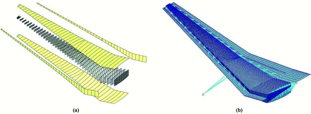
Wingbox model. (a) Wingbox designable patches for spars, ribs and skins. (b) Wing structural FE model and aerodynamic panelling.

The wingbox model is auto-meshed with in-house MATLAB and MSC/PATRAN scripts using shell elements for the skins, ribs and spars (for improved laminate principal stresses and strains calculations), and beam elements for the stiffeners. To emulate aircraft weight due to non-structural components, lumped masses connected to the spars via rigid body connectors with distributed loadings are employed for the fuel load, engine/nacelle set and leading and trailing-edge sub-structures. An additional balance lumped mass is placed at the aircraft centre of gravity (C.G.) to characterise fuselage, payload, and reserve fuel contributions to the aircraft overall inertia. The lumped masses for trailing-edge devices are placed approximately at the control hinge line.
The model is limited to a Maximum Take-Off Weight (MTOW) of approximately 255,000kg, with an Operational Empty Weight (OEW) of 137,900kg, 95,500kg of which are due to the fuselage and tail assemblies, 7,500kg to each engine/nacelle and approximately 10,000kg to the half-wing structure. A total of 1,200kg are used as non-structural mass for the leading-edge devices and 2,500kg for the trailing-edge controls and actuators (the actuator masses are assumed to be proportional to the flap area).
To allow for detailed variations in both material properties and thicknesses during the optimisation process, the structural Finite Element (FE) model is divided into various tailorable-zones, as shown in Fig. 2(a). Each wing skin features a total of 39 rib-bay patches. Similarly, 39 designable patches are used for each spar.
The aerodynamic panelling is divided into two lifting surfaces: a main wing and a tailplane used for static longitudinal trim calculations. The aerodynamic mesh consists of a total of 2,105 boxes evenly distributed in the spanwise direction. For the chordwise topology, a cosine distribution is used to accurately capture pressure variations at the wing leading and trailing-edges (see Fig. 2(b)). The wing jig-twist and aerofoil camber distributions are input via Direct Matrix Input (DMI) entries as a W2GJ NASTRAN matrix by changing the effective downwash angle of each aerodynamic element.
3.0 AEROELASTIC ANALYSIS AND STRUCTURAL STABILITY CALCULATIONS
In this work, NASTRAN routine 144 is used to perform longitudinal trim analyses and to compute static aeroelastic loads and aerostructural design metrics. NASTRAN implements the Doublet-Lattice subsonic lifting surface theory (DLM), which can estimate rigid and flexible aerodynamic loads. The choice of the aerodynamic solver is based on a trade-off between computational cost and accuracy of the solution. Advanced CFD techniques are known to capture important transonic effects better, such as the drag rise behaviour and shocks formation, though a substantial increase in computational cost is expected. Here, we use a much simpler, but faster, aerodynamic solver. Since the DLM is based on a linearised aerodynamic potential theory, the abovementioned transonic effects are all neglected, which reduces the accuracy of the predicted drag and aerodynamic loads. Consequently, care must be taken in interpreting the solutions found, as these are only acceptable as first-order estimates.
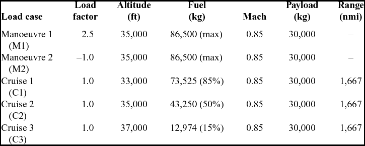
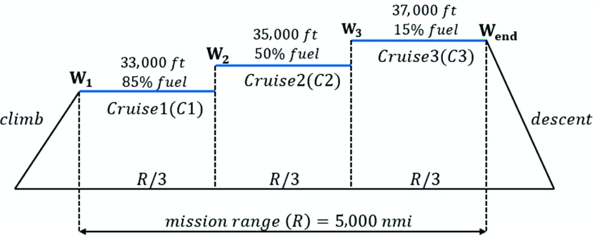
A total of five representative symmetric load cases (limited by computational resources) are considered in the optimisation problem as summarised in Table 2. The first two load cases are mainly for sizing purposes: a 2.5g pull-up and a -1.0g push-down manoeuvres at mid-cruise altitude and speed with maximum take-off weight. The last three load cases are used for fuel burn minimisation trade-off studies. The overall cruise profile assumes the shape of a “cruise-climb” mission (see Fig. 3) with increasing altitude for a constant Mach number as fuel is consumed. An aircraft payload (30,000kg) and mission range (5,000nmi) were chosen based on Ref. (Reference Liem, Kenway and Martins15).
Static aeroelastic load cases considered

Cruising flight mission profile divided into three phases.

The wingbox structural stability is evaluated via a linear buckling analysis (as implemented in NASTRAN solution 105) using the aerodynamic loads of the M1 and M2 load cases. The first five buckling load factors are evaluated and used as a design constraint as explained in Section 5.2.2.
3.1 Total drag dissipation estimate
For fuel burn calculations, an accurate and realistic estimation of the drag build-up for cruising flights is essential, because this can significantly influence the optimisation final solution. To address this issue, we account for profile drag and wave drag contributions as presented in Ref. (Reference Kennedy and Martins11). With this approach, wing profile and wave drag coefficients (C Dp and C Dc, respectively), which are otherwise not included in standard DLM, are estimated semi-empirically. This approach is used here as a first-order approximation of the aircraft wing drag. The lift-induced drag (C Dl) is estimated with a Trefftz-plane method as proposed in Ref. (Reference Kolonay and Eastep30). The profile drag is calculated as a quadratic function of the local lift coefficient (cl), so that
 $$\begin{equation}
{C_{{D_p}}} = \ {C_{{D_0}}}\left[ {1 + \frac{{0.38}}{{\cos {\Lambda _{le}}}}\left( {c_l^2} \right)} \right],
\end{equation}$$
where Λle is the wing leading-edge sweep angle. Differently from Ref. [11], here, the C D 0 coefficient used to estimate the profile drag, is calculated according to Ref. [37] as described next. This coefficient is related to zero-lift drag dissipations of viscous skin-friction nature, usually associated with flow separations or other similar flow instabilities. Its contribution to the total aircraft drag is proportional to viscous drag coefficient (Cf), form factor  $( {\cal F} )$ and wing wetted area ratio (S wetted/S), so that
 $$\begin{equation}
{C_{{D_0}}} = \ {C_f}{\cal F}\frac{{{S_{{\rm{wetted}}}}}}{S},
\end{equation}$$
where S is the wing planform area. In Equation (2), the viscous drag coefficient is calculated assuming a flat plate theory for turbulent flows and is given by
 $$\begin{equation}
{C_f} = \frac{{0.455}}{{{{\left( {\log R{e_x}} \right)}^{2.58}}{{\left( {1 + 0.144{M^2}} \right)}^{0.65}}}}.
\end{equation}$$
In Equation (3), M is the free-stream Mach number and Rex is the wing average Reynolds number estimated using the mean aerodynamic chord  $( {\bar{c}} )$, the component of the free-stream velocity (U 0) and the kinematic viscosity (ν)
 $$\begin{equation}
R{e_x} = \ \bar{c}{U_0}\cos {\Lambda _{le}}/\nu .
\end{equation}$$
The form factor  ${\cal F}$ accounts for the rise in wing skin-friction drag due to flow separations and is described as a function of the wing maximum thickness position (x/c)max, the thickness-to-chord ratio (t/c) spanwise variation and the geometric sweep angle of the maximum thickness line (Λt/c max). It can be calculated according to the relationship
 $$\begin{equation}
{\cal F} = \left[ {1 + \ \frac{{0.6}}{{{{\left( {x/c} \right)}_{{\rm{max}}}}}}\left( {\frac{t}{c}} \right) + \ 100{{\left( {\frac{t}{c}} \right)}^4}} \right]\left[ {1.34{M^{0.18}}{{\left( {{\rm{cos}}\left( {{\Lambda _{t/{c_{{\rm{max}}}}}}} \right)} \right)}^{0.28}}} \right]\ .
\end{equation}$$
The total aircraft drag coefficient results from the contributions of the profile drag, wave drag, lift-induced drag and additional losses (C D losses) due to non-modelled fuselage, vertical tail and other drag sources (a value of 100 drag counts is assumed for the C D losses contribution) such that
 $$\begin{equation}
{C_D} = \ {C_{{D_p}}} + {C_{{D_c}}} + \ {C_{{D_l}}} + {C_{{D_{{\rm{losses}}}}}}.
\end{equation}$$
4.0 FUNDAMENTAL LAMINATE CONSTITUTIVE EQUATIONS
According to Classical Laminated Plate Theory (CLPT)(Reference Jones38), a plate's two-dimensional displacement field, described in terms of its mid-plane strains and curvatures, can be related to resultant loads (generalised forces and moments) by the extensional (in-plane), A, bending-extension coupling, B, and bending (out-of-plane), D, stiffness matrices and is represented in compact form as
 $$\begin{equation}
\left[ {\begin{array}{@{}*{1}{c}@{}} {\bf N}\\ {\bf M} \end{array}} \right] = \left[ {\begin{array}{@{}*{2}{c}@{}} {\bf A}&{\bf B}\\ {\bf B}&{\bf D} \end{array}} \right]\left[ {\begin{array}{@{}*{1}{c}@{}} {{{\bm \varepsilon }^{\bf 0}}}\\ {\bm \kappa } \end{array}} \right].
\end{equation}$$
Equation (7) can be written more explicitly in terms of generalised forces, N = {Nx, Ny, Nxy}T; and moments, M = {Mx, My, Mxy}T; and related strains,  ${ {{\bm \varepsilon }}^{\bf 0}} = {\{ {\varepsilon _x^o,\varepsilon _y^o,\gamma _{xy}^o} \}^T}$; and curvatures,
 $ {{\bm \kappa }} = {\{ {{\kappa _x},{\kappa _y},{\kappa _{xy}}} \}^T}$, such that
 $$\begin{equation}
\left\{ {\begin{array}{@{}*{1}{c}@{}} {\begin{array}{@{}*{1}{c}@{}} {{N_x}}\\ {{N_y}}\\ {{N_{xy}}} \end{array}}\\ {\begin{array}{@{}*{1}{c}@{}} {{M_x}}\\ {{M_y}}\\ {{M_{xy}}} \end{array}} \end{array}} \right\} = \left[ {\begin{array}{@{}*{3}{c}@{}} {\begin{array}{@{}*{3}{c}@{}} {{A_{11}}}&{{A_{12}}}&{{A_{16}}}\\ {}&{{A_{22}}}&{{A_{26}}}\\ {sym}&{}&{{A_{66}}} \end{array}}&{\begin{array}{@{}*{3}{c}@{}} {{B_{11}}}&{{B_{12}}}&{{B_{16}}}\\ {}&{{B_{22}}}&{{B_{26}}}\\ {sym}&{}&{{B_{66}}} \end{array}}\\ {\begin{array}{@{}*{3}{c}@{}} {{B_{11}}}&{{B_{12}}}&{{B_{16}}}\\ {}&{{B_{22}}}&{{B_{26}}}\\ {sym}&{}&{{B_{66}}} \end{array}}&{\begin{array}{@{}*{3}{c}@{}} {{D_{11}}}&{{D_{12}}}&{{D_{16}}}\\ {}&{{D_{22}}}&{{D_{26}}}\\ {sym}&{}&{{D_{66}}} \end{array}} \end{array}} \right]\left\{ {\begin{array}{@{}*{1}{c}@{}} {\begin{array}{@{}*{1}{c}@{}} {\varepsilon _x^o}\\ {\varepsilon _y^o}\\ {\gamma _{xy}^o} \end{array}}\\ {\begin{array}{@{}*{1}{c}@{}} {{\kappa _x}}\\ {{\kappa _y}}\\ {{\kappa _{xy}}} \end{array}} \end{array}} \right\},
\end{equation}$$
where N and M are obtained by integrating stresses through the laminate thickness and Aij, Bij, and Dij, with i,j= 1, 2, 6, are functions of material properties and stacking sequence.
Examination of Equation (8) shows insight on the type of coupling produced by a laminate and the significance of stiffness matrices as a means of passive aeroelastic tailoring. Shear-extension coupling may occur due to the presence of A 16 and A 26, which relate in-plane normal forces with shear deformation and shear forces with in-plane elongations. Similarly, extension-extension coupling can be achieved with A 12, which relates normal forces with normal elongations in the principal directions. In balanced laminates (i.e. for every ply at an angle θ, there must be a ply with orientation − θ within the stacking sequence) the elements A 16 = A 26 = 0, and thus, shear-extension coupling is not possible.
The out-of-plane elements D 16 and D 26 measure the bend-twist coupling, which causes applied bending moments to twist the laminate, and resultant twist moments to produce out-of-plane curvatures. Finally, the out-of-plane stiffness D 12 produces bending-bending coupling, causing resultant moments to induce curvatures in the direction perpendicular to the applied load. In this work, couplings induced by bending-extension stiffness coefficients are not considered for reasons discussed in Section 4.1.
In aerostructural optimisation problems, wingbox structures are commonly subdivided into a number of tailorable-zones encompassing rib and/or stringer-bay patches. A complete detailed parameterisation of composite structures at the stacking sequence level often results in an impractical number of design variables, which may bring about computational limitations. Tsai et al.(Reference Tsai, Halpin and Pagano39) and Tsai and Hahn(Reference Tsai and Hahn40) introduced an alternative formulation for the A, B, D matrices that is beneficial for optimisation purposes because it reduces the total number of design variables significantly. Additionally, its continuous nature makes it suitable for gradient-based optimisers. The in-plane and out-of-plane stiffnesses can then be expressed as linear functions of five material invariants (which can be calculated from the material properties presented in Table 1), Uk, and eight (twelve when B ≠ 0) lamination parameters, ξji, with i = 1, . . .4, j = A, D, and k = 1, . . .5, such that
 $$\begin{equation}
\left\{ {\begin{array}{@{}*{1}{c}@{}} {\begin{array}{@{}*{1}{c}@{}} {{A_{11}}}\\ {{A_{22}}}\\ {{A_{12}}} \end{array}}\\ {\begin{array}{@{}*{1}{c}@{}} {{A_{66}}}\\ {{A_{16}}}\\ {{A_{26}}} \end{array}} \end{array}} \right\} = h\left[ {\begin{array}{@{}*{2}{c}@{}} {\begin{array}{@{}*{2}{c}@{}} 1&{\ \xi _1^A}\\ 1&{\ - \xi _1^A}\\ 0&{\ 0} \end{array}}&{\begin{array}{@{}*{3}{c}@{}} {\ \xi _3^A}&0&0\\ {\ \xi _3^A}&0&0\\ { - \xi _3^A}&1&0 \end{array}}\\ {\begin{array}{@{}*{2}{c}@{}} {\ 0}&{\ 0}\\ {\ 0}&{\xi _2^A/2}\\ {\ 0}&{\xi _2^A/2} \end{array}}&{\begin{array}{@{}*{3}{c}@{}} { - \xi _3^A}&0&1\\ {\ \xi _4^A}&0&0\\ {-\xi _4^A}&0&0 \end{array}} \end{array}} \right]\left\{ {\begin{array}{@{}*{1}{c}@{}} {\begin{array}{@{}*{1}{c}@{}} {{U_1}}\\ {{U_2}}\\ {{U_3}} \end{array}}\\ {\begin{array}{@{}*{1}{c}@{}} {{U_4}}\\ {{U_5}} \end{array}} \end{array}} \right\},
\end{equation}$$ \\
 $$\begin{equation}
\left\{ {\begin{array}{@{}*{1}{c}@{}} {\begin{array}{@{}*{1}{c}@{}} {{D_{11}}}\\ {{D_{22}}}\\ {{D_{12}}} \end{array}}\\ {\begin{array}{@{}*{1}{c}@{}} {{D_{66}}}\\ {{D_{16}}}\\ {{D_{26}}} \end{array}} \end{array}} \right\} = \frac{{{h^3}}}{{12}}\left[ {\begin{array}{@{}*{2}{c}@{}} {\begin{array}{@{}*{2}{c}@{}} 1&{\ \xi _1^D}\\ 1&{\ - \xi _1^D}\\ 0&{\ 0} \end{array}}&{\begin{array}{@{}*{3}{c}@{}} {\ \xi _3^D}&0&0\\ {\ \xi _3^D}&0&0\\ { - \xi _3^D}&1&0 \end{array}}\\ {\begin{array}{@{}*{2}{c}@{}} {\ 0}&{\ 0}\\ {\ 0}&{\xi _2^D/2}\\ {\ 0}&{\xi _2^D/2} \end{array}}&{\begin{array}{@{}*{3}{c}@{}} { - \xi _3^D}&0&1\\ {\ \xi _4^D}&0&0\\ {-\xi _4^D}&0&0 \end{array}} \end{array}} \right]\left\{ {\begin{array}{@{}*{1}{c}@{}} {\begin{array}{@{}*{1}{c}@{}} {{U_1}}\\ {{U_2}}\\ {{U_3}} \end{array}}\\ {\begin{array}{@{}*{1}{c}@{}} {{U_4}}\\ {{U_5}} \end{array}} \end{array}} \right\},
\end{equation}$$
 $$\begin{equation}
\xi _{\left[ {1,2,3,4} \right]}^A = {\rm{\ }}\frac{1}{h}\mathop \smallint \limits_{ - h/2}^{h/2} \left[ {{\rm{cos}}2\theta ,{\rm{sin}}2\theta ,{\rm{cos}}4\theta ,{\rm{sin}}4\theta } \right]dz,
\end{equation}$$\\
 $$\begin{equation}
\xi _{\left[ {1,2,3,4} \right]}^D = {\rm{\ }}\frac{{12}}{{{h^3}}}\mathop \smallint \limits_{ - h/2}^{h/2} \left[ {{\rm{cos}}2\theta ,{\rm{sin}}2\theta ,{\rm{cos}}4\theta ,{\rm{sin}}4\theta } \right]{z^2}dz,
\end{equation}$$
4.1 Laminate design guidelines
Over the last decades, the search for more structurally efficient materials, combined with a number of lessons learned within the aerospace industry, resulted in the development of a series of composite design guidelines. These guidelines may differ from organisation to organisation but serve the purpose of offering sufficient confidence to the design of manufacturable composite airframes. Moreover, these guidelines are a means to provide design solutions (or restrictions) that satisfy certification purposes and production requirements linked to manufacturing limitations.
Reference (Reference Bloomfield, Diaconu and Weaver41) provides a more comprehensive discussion about the development and justification of these “rules of thumb”. The most common design guidelines are implemented in this work.
(a) Only unidirectional plies restricted to four main directions (i.e. 0°, ±45°, and 90°) are allowed in the laminate stacking sequence.
(b) Laminates must have a minimum of 10% of their plies oriented in each one of the four principal directions.
(c) A maximum of 60% of plies oriented in any direction is allowed in the laminate.
(d) At least one pair of ±45° plies should be placed in the laminate outer plies.
(e) The laminate must be balanced (A 16 = 0 and A 26 = 0)to eliminate shear-extension coupling, i.e. the number of −45° and +45° plies must be the same.
(f) Laminate sequences must be symmetric about their middle surface in order to remove bending-extension coupling (Bij = 0).
(g) A maximum of four plies of the same orientation and thickness can be stacked together. This is to prevent matrix-cracking between layers.
(h) All layers of the thinner laminate must be present in all other wing skin panels. In other words, the laminate must share layers between adjacent panels in order to fulfil blending constraints.
Note that, in particular, design guideline (e) limits considerably the tailoring capability of the composite skins by eliminating shear-extension coupling. For this reason, the laminate configuration adopted here can be unbalanced (A 16 ≠ 0 and A 26 ≠ 0).
4.2 Criteria for lamination parameters feasibility
As defined by Equations (11) and (12), lamination parameters are continuous variables of trigonometric characterisation, and therefore, they must be constrained to mathematically feasible regions that are enclosed by the relationships suggested in Refs (Reference Bloomfield, Diaconu and Weaver42,Reference Liu, Toropov, Querin and Barton43). These are
 $$\begin{equation}
\begin{array}{@{}l@{}} 2\left( {1 + \xi _3^i} \right){\left( {\xi _2^i} \right)^2} - 4\xi _1^i\xi _2^i\xi _4^i + {\left( {\xi _4^i} \right)^2} \le \left( {\xi _3^i - 2{{\left( {\xi _1^i} \right)}^2} + 1} \right)\left( {1 - \xi _3^i} \right),\\ \quad \quad \quad \quad \quad \quad \quad \quad \quad {\left( {\xi _1^i} \right)^2} + {\left( {\xi _2^i} \right)^2} \le 1,\\ \quad \quad \quad \quad {\left( {\xi _j^A - 1} \right)^4} - 4\left( {\xi _j^A - 1} \right)\left( {\xi _j^D - 1} \right) \le 0,\\ \quad \quad \quad \quad {\left( {\xi _j^A + 1} \right)^4}\ - 4\left( {\xi _j^A + 1} \right)\left( {\xi _j^D + 1} \right) \le 0,\\ \quad \quad \quad \quad \quad \quad \quad \quad - 1 \le \xi _j^i \le 1, \end{array}
\end{equation}$$
where i = A,D and j = 1, . . ., 4. These inequalities are employed in the optimisation problem as nonlinear constraints in order to ensure retrieval of feasible stacking sequences.
In order to comply with the manufacturing guidelines (b) and (c) of Section 4.1, additional relations adapted from Ref. 44 are implemented as design constraints at lamination parameter level so that
 $$\begin{equation}
\begin{array}{@{}l@{}} 0^\circ \ {\rm{ply}}\ \% :\quad 0.1 \le \left( {\xi _3^A + 2\xi _1^A + 1} \right)/4 \le 0.6,\\ 90^\circ \ {\rm{ply}}\ \% :\quad 0.1 \le \left( {\xi _3^A - 2\xi _1^A + 1} \right)/4 \le 0.6,\\ + 45^\circ \ {\rm{ply}}\ \% :\quad 0.1 \le \left( {1 + 2\xi _2^A - \xi _3^A} \right)/4 \le 0.6,\\ - 45^\circ \ {\rm{ply}}\ \% :\quad 0.1 \le \left( {1 - 2\xi _2^A - \xi _3^A} \right)/4 \le 0.6. \end{array}
\end{equation}$$
5.0 OPTIMISATION PROBLEM DESCRIPTION
In this section, we investigate the synergies and trade-offs between passive aeroelastic tailoring and adaptive aeroelastic deformation of a representative composite wing for fuel burn minimisation by optimising laminate thickness and stiffness distributions, jig-twist shape and controls deflections through different segments of a nominal cruise mission and critical symmetric manoeuvres.
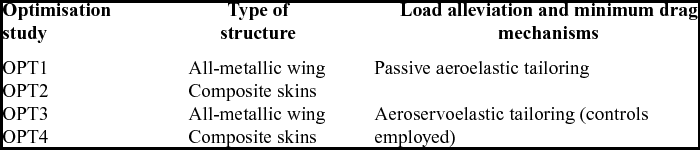
A total of four design studies, labelled “OPT” 1 to 4, are performed. The first and second design studies tailor the wingbox structure for passive adaptation (controls are held fixed with zero deflection) for two different wing configurations, i.e. a metallic and a hybrid wing with composite skins, respectively. The aforementioned exercise is repeated in OPT 3 and OPT 4 with the trailing-edge controls employed as a mechanism for adaptive load alleviation for a 2.5g pull-up manoeuvre and to minimise the overall drag for cruise (load cases as described in Section 3). These optimisation studies are summarised in Table 3.
Optimisation study cases

The laminate ply-book (detailed ply orientations and stacking sequence) of the composite designs are retrieved via a separate optimisation level. Since the conversion from lamination parameter space to stacking sequence space may entail some stiffness discrepancies, the aerostructural performance of the designs defined with detailed ply-books is then assessed and benchmarked by comparing it against OPT 1 to 4.
5.1 Optimisation workflow
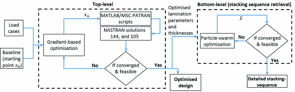
The optimisation workflow implemented in this work is represented in Fig. 4. The optimisation process is divided in two separate and consecutive levels (there is no feedback response between the first and second level), distinguished as “top-level” and “bottom-level” optimisations.
Bi-level optimisation workflow.

The top-level optimisation starts with the baseline design (x 0) and the load cases described in Sections 2 and 3 as input and uses a gradient-based optimiser to calculate aeroelastic sensitivities of the objective function and design constraints, with respect to the design variables. At this level, a series of in-house MSC/PATRAN and MATLAB scripts are used to generate input files for the aeroelastic calculations (NASTRAN routines 144 and 105). The optimisation continues until it reaches one of the stopping criteria (i.e. thresholds for the optimisation step-size and first-order optimality measure).
Based on the lamination parameters and thicknesses from the top-level optimisation, the bottom-level optimisation uses a particle-swarm algorithm to retrieve feasible stacking sequences and detailed wing skin ply-books with blending considerations. Both optimisation levels are described in more detail in the following sections.
5.2 Top-level optimisation using a gradient-based algorithm
The top-level optimisation problem is solved using MATLAB's gradient-based algorithm fmincon. Gradients of the objective function and design constraints with respect to the design variables are calculated via forward finite differences with a Sequential Quadratic Programming (SQP) approach(Reference Nocedal and Wright45).
Matlab's implementation of the SQP method is purposely designed for nonlinearly constrained optimisation problems being efficient in terms of memory usage and execution time. When the constraints are not satisfied, the SQP solver uses the penalty function approach that combines the objective and constraint functions into a single merit function, which is then minimised with relaxed bounds. This approach results in a better understanding of the conflicting trade-offs that governs the optimisation problem, usually resulting in a superior solution when compared to other gradient-based approaches. The Hessian of the Lagrangian is updated at every iteration using a quasi-Newton method to resolve a quadratic programming sub-problem in order to determine the line search direction.
The next sections present the design variables and design constraints parameterisation in detail as well as the objective function adopted for the bi-level optimisation.
5.2.1 Design variables parameterisation
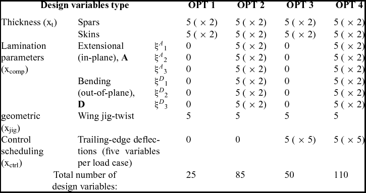
The top-level optimisation uses four different sets of continuous design variables divided into: (1) thicknesses of the main wing sub-structure components (x t), i.e. spars and skins; (2) in-plane and out-of-plane lamination parameters (x comp) for the composite skins of OPT 2 and OPT 4; (3) geometric variables (x jig) which define the wing jig-twist shape; and (4) trailing-edge control deflections (x ctrl) for each load case considered in the analysis.
For all design variables, a Piecewise Cubic Hermite Interpolating Polynomial (PCHIP) technique is used to describe multiple design properties variations in the spanwise direction, i.e. one PCHIP for thickness of each spar and each skin, lamination parameters ξA, D[1, 2, 3] of each skin, jig-twist and trailing-edge control rotations of each load case. This technique fits a piecewise polynomial passing through a fixed number of equally spaced control points placed from wing root to wingtip. For thicknesses and lamination parameters, the PCHIP is interpolated over 39 designable patches (as shown in Fig. 2(a)); jig-twist variables are interpolated at 84 aerodynamic strips and four structural sections (root, tip and spar breaks), whereas control surface rotations are interpolated at twelve discrete control surfaces.
Using the PCHIP technique to describe variations in properties along the wing structure significantly reduces the number of design variables, which is convenient for the optimisation algorithm chosen, because the computational cost of each iteration is proportional to n + 1 function evaluations, where n is the total number of design variables. Nonetheless, the quality of the final solution is strongly affected by the number and location of the control points.
It is found that six control points for thicknesses and lamination parameters (from which only the first five are used as design variables) and five control points for the remaining design variables offers a good trade-off between computational cost and optimality of the solutions. Note that, for thicknesses and lamination parameters, the sixth control point, placed at the wingtip, is fixed at 3mm and zero, respectively – initial studies showed no sensible variation in the objective function if this control point was used as a design variable. Furthermore, this special type of piecewise parameterisation guarantees continuity and smoothness of structural properties along the wing, which, presumably, favours the design of blended composite wing skins.
For all of the optimisation study cases considered here, the design variables defining the thickness distribution are allowed to range from 3mm and 30mm. In-plane and out-of-plane lamination parameters are bounded by the feasibility relationships of Equations (13) and (14) discussed in Section 4.2. Jig-twist variables can vary from 4° to −1° whilst control surface deflections range from –8° to 8°. The design variables are standardised and nondimensionalised to vary between −1 and 1 to assure a good convergence rate and to avoid insensitiveness to step-size variations of one or more of the variables, because their absolute order of magnitude may differ widely otherwise. Table 4 summarises the number and type of design variables used in the optimisation problems.
Set of design variables used in the top-level optimisation

5.2.2 Design constraints
In order to restrict the design to feasible and physically meaningful solutions, we use a number of design constraints in the top-level optimisation analysis. To comply with the limitations of the aeroelastic solver chosen, the first set of design constraints narrows the wing structural deformations to the linear elastic behaviour only. This is done by defining two main deformation constraints: (a) a maximum twist angle and (b) a maximum bending deflection. These constraints are written as
 $$\begin{equation}
{C_{{\rm{twist}}}} = \frac{{{\theta _{{\rm{tip}}}}}}{{{\theta _{{\rm{allowed}}}}}} \le 1,
\end{equation}$$ \\
 $$\begin{equation}
{C_{{\rm{bending}}}} = \frac{{{z_{{\rm{tip}}}}}}{{{z_{{\rm{allowed}}}}}} \le 1,
\end{equation}$$
Buckling load factors, composite principal stresses and strains, and Mises-based stresses and strains for metallic parts are constrained with the Kreisselmer-Steinhauser (KS) aggregation technique(Reference Kreisselmeier and Steinhauser46,Reference Poon and Martins47) . The aggregation formula used to constrain principal stresses and strains is given by
 $$\begin{equation}
K{S_{{\rm{metric}}}} = \ {C_{{\rm{max}}}} + \frac{1}{{{\rho _{KS}}}}\ln \left[ {\mathop \sum \limits_{i = 1}^n {{\rm{e}}^{{\rho _{KS}}\left( {{C_i} - \ {C_{{\rm{max}}}}} \right)}}} \right],
\end{equation}$$
where Ci is the ratio between the constraint metric for the i th finite element and its allowed value (yield stress or maximum strain) and C max is the maximum constraint metric in the current design point. The parameter ρKS represents the aggregation factor which is set to 50. A KS constraint is said to be violated when its value is greater than one. For each aeroelastic load case, Equation (17) is used to aggregate (a) major and minor principal stresses and strains for the laminated wing skins, and (b) equivalent von Mises stresses and strains for the metallic sub-structures. For buckling load factors, the first five eigenvalues of the most critical load cases are aggregated with a modified KS formula as proposed in Ref. Reference Dunning, Stanford and Kim21.
 $$\begin{equation}
K{S_{{\rm{Buckling}}}} = \ 2 - {\lambda _{{\rm{min}}}} + \frac{1}{{{\rho _{KS}}}}\ln \left[ {\mathop \sum \limits_{i = 1}^n {{\rm{e}}^{{\rho _{KS}}\left( {{\lambda _{{\rm{min}}}} - \ {\lambda _i}} \right)}}} \right],
\end{equation}$$
where λmin is the minimum buckling load factor. This technique is beneficial for optimisation purposes because it simplifies and reduces total number of design constraints considerably (usually at the finite element level), combining them into a single parameter per constrained design metric. It may also improve robustness against the switching of critical buckling modes at reduced computational cost(Reference Dunning, Stanford and Kim21).
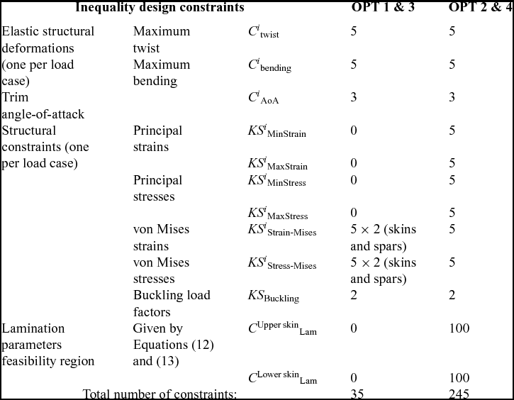
The use of trailing-edge controls can alter the resulting trim Angle-of-Attack (AoA) to values lower than those acceptable for passenger comfort (i.e. slightly negative AoA). For this reason, the trim AoA for all cruise flight conditions is constrained to a minimum of 1.5°. Table 5 summarises the number and type of design constraints used in the optimisation problems. Note that lamination parameters feasibility relationships are applied at each control point, whereas KS constraints are used for each load case considered (except for KS Buckling, where only the buckling loads of the M1 and M2 manoeuvres are of interest).
Set of design constraints used in the top-level optimisation

5.2.3 Objective function
The objective function used in the top-level optimisation is to minimise the total fuel burned during cruise. For a particular mission range, the fuel consumed can be estimated using the well-known Breguet range equation assuming that the Thrust Specific Fuel Consumption (TSFC), the aircraft speed (U 0) and the lift efficiency (CL/CD) remain constant along a given cruise segment. Under these assumptions, the range equation is
 $$\begin{equation}
R = \ \frac{{{U_0}}}{{TSFC}}\left( {\frac{{{C_L}}}{{{C_D}}}} \right)\ln \left( {\frac{{{W_{{\rm{begin}}}}}}{{{W_{{\rm{end}}}}}}} \right),
\end{equation}$$
where the TSFC is taken as a function of the altitude, decreasing 1% for every increment of 2,500ft in the flight level (as a reference, a value of 0.53lb/(lbf·h) is adopted for 35,000ft). Equation (19) can be rearranged in terms of fuel burned for given cruise segment (FBi) and written as
 $$\begin{equation}
F{B_i} = \ {W_i} - {W_{i + 1}} = {W_i}\left[ {1 - \exp \left( { - R{S_i}} \right)} \right],
\end{equation}$$
where Wi and W i + 1 are the initial and final aircraft weight of the i th cruise flight segment, respectively, and the parameter RSi is
 $$\begin{equation}
R{S_i} = \ \frac{{{R_i}TSF{C_i}}}{{{U_0}{{\left( {{C_L}/{C_D}} \right)}_i}}}.
\end{equation}$$
From Equations (20) and (21), it can be shown that the total fuel consumed over the entirety of the cruise-climb mission (for n cruise segments) is a function of the initial cruise weight (W 1) and the summation of RSi parameters, as in
 $$\begin{equation}
F{B_{{\rm{total}}}} = \ {W_1}\left[ {1 - {\rm{exp}}\left( { - \mathop \sum \limits_{i = 1}^n R{S_i}} \right)} \right].
\end{equation}$$
The objective function is obtained from Equation (22) by normalising to the order of unity using a reference baseline value
 $$\begin{equation}
f_{{\rm{obj}}}^{{\rm{top}} - {\rm{level}}}\left( {{\bf x}} \right) = \ F{B_{{\rm{total}}}}/F{B_{{\rm{baseline}}}},
\end{equation}$$
In conclusion, the top-level optimisation problem can be formulated as
 $$\begin{equation*}
\mathop {{\rm{minimise}}}\limits_{{{\bf x}} \in {\rm{\Omega }}} f_{{\rm{obj}}}^{{\rm{top}} - {\rm{level}}}\left( {{\bf x}} \right)
\end{equation*}$$
 $$\begin{equation*}
{\rm{with}}\;{\rm{respect}}\;{\rm{to}}:{{\bf x}} = {\left\{ {{x_{\rm{t}}},{x_{{\rm{comp}}}},{x_{{\rm{jig}}}},{x_{{\rm{crtl}}}}} \right\}^T}\;{\rm{and}}\;{\rm{\Omega }} = \left\{ {{{\bf x}}|C\left( {{\bf x}} \right) \le 0\ } \right\}
\end{equation*}$$
 $$\begin{equation}
{\rm{such}}\;{\rm{that}}\;C\left( {{\bf x}} \right) = \left\{ {\begin{array}{@{}*{1}{c}@{}} {KS_{{\rm{MinStrain}}}^i - 1;}\\[5pt] {KS_{{\rm{MaxStrain}}}^i - 1;}\\[5pt] {KS_{{\rm{MinStress}}}^i - 1;}\\[5pt] {KS_{{\rm{MaxStress}}}^i - 1;}\\[5pt] {\ \ \ KS_{{\rm{Stress - Mises}}}^i - 1;}\\[5pt] {\ \ \ KS_{{\rm{Strain - Mises}}}^i - 1;}\\[5pt] {KS_{{\rm{Buckling}}}^{i = 1,2} - 1;}\\[5pt] {\ \ \ C_{{\rm{AoA}}\ \ \ \ }^i - 1;}\\[5pt] {C_{{\rm{twist}}}^i - 1;}\\[5pt] {C_{{\rm{bending}}}^i - 1;}\\[5pt] {C_{{\rm{bending}}}^i}\\ { - 1 \le {{\bf x}} \le 1} \end{array}} \right.\quad \quad i = 1,\ \ldots ,{N_L},
\end{equation}$$
where x = {x t, x comp, x ctrl, x jig}T is the vector of design variables, C(x) are the design constraints, and NL is the number of load cases.
It is worth mentioning that the optimisation studies are conducted via a sequential optimisation approach. For wings augmented by trailing-edge control surfaces, the first step is to find the optimal control scheduling that would yield minimum summation of the KS metrics for manoeuvre load cases M1 and M2. At this step, only control deflections are used as design variables. The second step (only applicable for composite wings) retains fixed optimal control deflections for load alleviation and minimises KS metrics for the most critical load case, this time using only lamination parameters as design variables. The final step handles all design variables simultaneously and minimises fuel burn as previously mentioned. This approach is not only useful in providing insight of the physical behaviours that govern the designs but also guarantees feasibility of the optimisation starting point. Moreover, it was found that this sequential optimisation technique solves the optimisation problem in a more efficient manner, requiring fewer iterations to converge when compared to a random starting point, effectively searching the design space and yielding a better solution than the single step approach.
5.3 Bottom-level optimisation for stacking sequence retrieval for blended laminates
The stacking sequence retrieval of feasible laminates with blending considerations from lamination parameters is achieved by a separate bottom-level optimisation. This second level optimisation targets in-plane and out-of-plane lamination parameters and the thicknesses output from the top-level solution.
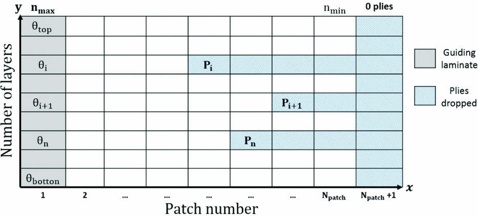
In this work, we propose an approach that combines the idea of Stacking Sequence Tables (SST) as proposed by Ref. 48 and the guide-based blending approach, first introduced in Ref. Reference Adams, Watson, Gürdal and Anderson-Cook49. Here, differently from Ref. 48 , SSTs are mapped into a Cartesian coordinate system as shown in Fig. 5. Starting from the thicker laminate (i.e. the guiding laminate), the “x-coordinate” denotes the wing skin patch number, while the “y-coordinate” represents the ply position relative to the laminate's mid-surface. These coordinates are restricted to the set of natural numbers ( $\mathbb{N}$) only. As in Ref. Reference Adams, Watson, Gürdal and Anderson-Cook49, the panels' stacking sequences are derived from a thicker guiding stack by dropping off plies at specific locations within the laminate. In Fig. 5, each point Pi specifies a pair of numerical coordinates, which represent drop-off locations. From that point, a layer is removed from all thinner patches adjacent to the guide laminate.
Rectangular coordinate system merged with an SST.

The representation of a SST as a rectangular coordinate system allows the ply drop-offs x and y coordinates to be used as integer design variables along with the ply angles of the guiding laminate. The total number of design variables is 3n (n ply angles, n “x-coordinates”, and n “y-coordinates”), where n represents the number of layers of the guide-laminate. The problem is constrained by the design guidelines developed in Section 4.2. For this bottom-level optimisation, we chose a particle swarm optimisation (PSO) algorithm, which produced attainable solutions at a reduced computational cost when compared to other evolutionary optimisation algorithms.
The objective function is a weighted sum of root square differences between the top-level lamination parameters and thicknesses ξA, Dj, target and t p, target, respectively, and the lamination parameters and thicknesses calculated at the n th PSO iteration such that
 $$\begin{eqnarray}
f_{{\rm{obj}}}^{{\rm{bottom}} - {\rm{level}}}\left( {\bar{x}} \right) & = & {\alpha _1}\sqrt {\mathop \sum \limits_{j = 1}^4 {{\left( {\xi _j^{\rm{A}} - \xi _{j,{\rm{target}}}^{\rm{A}}} \right)}^2}} + {\alpha _2}\sqrt {\mathop \sum \limits_{j = 1}^4 {{\left( {\xi _j^{\rm{D}} - \xi _{j,{\rm{target}}}^{\rm{D}}} \right)}^2}} \nonumber\\
&& +\, {\alpha _3}\sqrt {\mathop \sum \limits_{p = 1}^{{N_p}} {{\left( {{t_p} - {t_{p,{\rm{target}}}}} \right)}^2}} ,
\end{eqnarray}$$
where the objective function is scaled to the order of unity by suitably choosing the weighting factors αi, and Np is the number of wing skin patches. In particular, it is found that α1 =α2 = 0.275 and α3 = 0.45 would yield reasonable results.
6.0 RESULTS DISCUSSION
This section contains the results obtained for six different design studies. In addition to those described in Table 3 (OPTs 1, 2, 3 and 4), here we discuss the aerostructural performance of the composite designs with stacking sequences retrieved with the second-level optimisation. We label these designs as OPT 2 SSr and OPT 4 SSr, respectively, where SSr stands for Stacking Sequence Retrieved.
Aerostructural performance benefits, in terms of load alleviation and fuel burn minimisation, of the composite wing with full-span trailing-edge controls are demonstrated by assessing the designs produced by the optimisation algorithm described in Section 5. Note that all the results presented are considered to be local optima, though different optimisation starting points did, in general, reveal similar trade-offs with minor variations in the objective function.
6.1 Composite stiffnesses
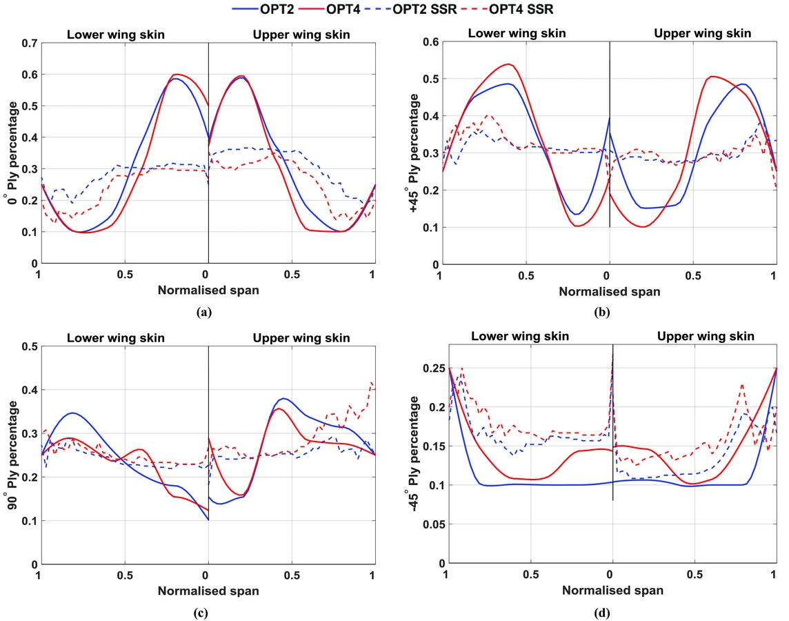
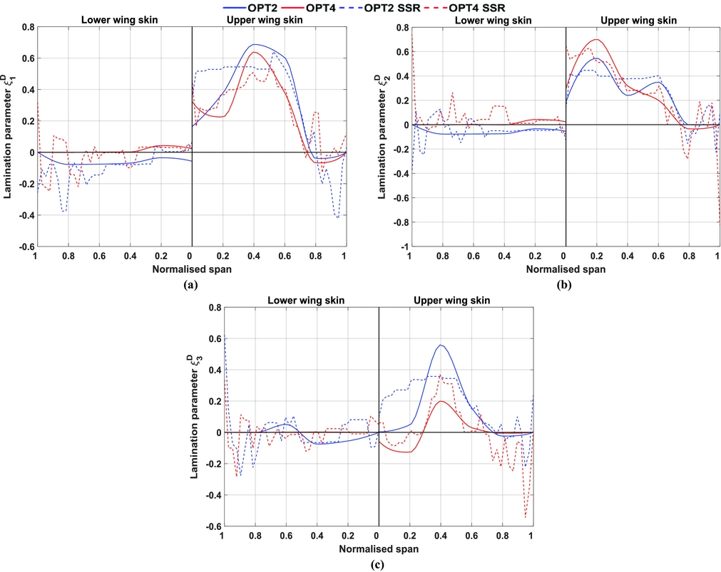
The out-of-plane lamination parameters obtained in the top-level optimisation for both the aeroelastically tailored and the aeroservoelastically tailored wings are shown in Fig. 7, along with the lamination parameters retrieved after blending constraints are applied. In-plane anisotropy is shown in Fig. 6 in terms of ply percentages (given by Equation (14)) distribution along the wing semi-span.
Optimised ply percentage distributions. (a) 0° plies. (b) + 45° plies. (c) 90° plies. (d) − 45° plies.

Optimised out-of-plane lamination parameters. (a) ξD1. (b) ξD2. (c) ξD3.

It is noted that both the upper and lower skins of OPT2 and OPT4 are mostly unbalanced featuring non-negligible values of + 45° and ξD2. These terms are respectively linked to the skins membrane and bending anisotropy. In general, both wings showed similar ply distributions with more 0° plies allocated towards the wing root (mostly at 20% of the semi-span) nearly reaching the upper bound of 60% with smoothly increasing amounts of + 45° towards the wing tip. This design trend indicates that the solver effectively aligns ply directions with the wing load path and uses the bend-twist coupling as a passive means for inducing the washout mechanism, which alleviates the aerodynamic loads allowing for more material to be removed from the outer skins and spars. It is thought that − 45° and 90° plies are mainly used to redistribute localised high strain areas at the spar breaks, particularly at the inner trailing-edge spar of OPT4 and at the edge between the outer front spar and lower wing skin of OPT2. Note that for most of the wing semi-span, there are a minimum number of − 45° plies (10%).
Upon further analysis it is observed that in comparison to the passively tailored skin of OPT2, OPT4 has greater shear-extension coupling inboard along the wing semi-span. This is evidenced for both upper and lower skins by the values of + 45°, which govern the laminate stiffnesses A 16and A 26. Similarly, after 20% of the semi-span, lower 0° ply percentages are found in the aeroservoelastically tailored composite wing. This result can be explained by the optimal control deflection scheduling for the symmetric 2.5g manoeuvre shown in Fig. 12. The trailing-edge downwards rotations of the inner wing flaps move the local centre of pressure aft inducing a torque on the wingbox, which in turn shift torsional loads further inboard towards the wing semi-span. Though this difference is not substantial, it is thought that increasing control surface's area and/or control surface rotation would, presumably, enhance this effect compelling the optimiser to allocate additional + 45° plies inboard the wing when compared to the passive counterpart.
Conversely, out-of-plane couplings (see Fig. 7) are stronger when adaptive control surfaces are not brought into the problem and are mainly used to improve the buckling strength in the wing root and mid-span areas. Inboard along the OPT2 wing, greater positive stiffnesses, linked to lamination parameters ξD1 and ξD3, are observed for the upper wing skin. For both composites wings, buckling constraints of the lower skins are inactive so that the out-of-plane lamination parameters are mainly used to attain feasibility of Equation (13), which are found to be active for both skins.
The lamination parameters obtained from the bottom-level optimisation and corresponding to feasible stacking sequences with blending constraints applied show significant deviations from the target stiffnesses (obtained in the first-level optimisation). Nonetheless, the impact of these deviations on the overall structural response is limited and detailed in the remainder of this section.
6.2 Thickness and strain distributions
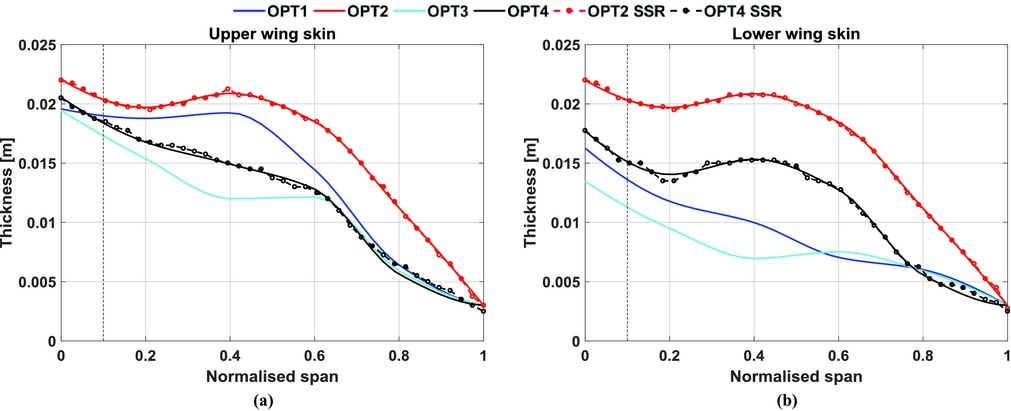
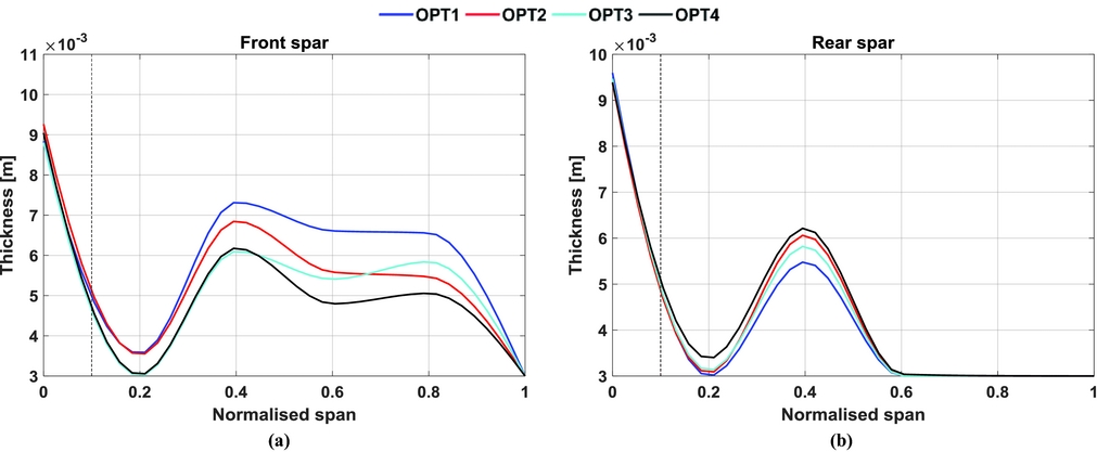
Optimised shell thicknesses for wing skins and spars are shown in Figs. 8 and 9. For all designs, the upper skins are thicker than the lower skins, indicating that the 2.5g pull-up manoeuvre buckling constraint is a strong design driver. In comparison to the passive adaptive wings, both control-actuated designs have substantially thinner skins and spars, marking a considerable weight reduction. In general, skin peak thicknesses are achieved approximately at the wing root and at the innermost 40% of the semi-span. Comparing OPT2 and OPT4 upper skin thicknesses, one can note that substantial weight reduction was achieved mainly by removing material outboard the first 20% of the wing semi-span. A similar design trend is observed when comparing OPT1 and OPT3 cases. It is found that the thickness sizing for the metallic wings is mainly driven by active buckling constraints of the load cases M1 and M2, whereas for both composite wings, principal strains of the lower wing skin and 2.5g pull-up manoeuvre buckling constraint are the main design drivers.
Optimised wing skin thickness distributions. (a) Upper wing skin thickness distribution. (b) Lower wing skin thickness distribution.

Optimised spars thickness distributions. (a) Front spar. (b) Rear spar.

The thickness profiles for the rear spars in OPT3 and OPT4 are similar in magnitude and approximately constant after the wing Yehudi break location. Note that, in all the optimised solutions, heavier front spars than the rear spars were achieved, possibly due to 2.5g torsional loads that induce higher stresses locally, with this being more evident for the spars of OPT1and OPT3. Moreover, the stiffer front spar creates a bend-twist coupling that induces a washout effect by shifting the flexural axis forward, further alleviating the wing loads. This effect is less prominent for the composite wing since it uses in-plane anisotropy on the skins to produce the same effect in a more efficient way.
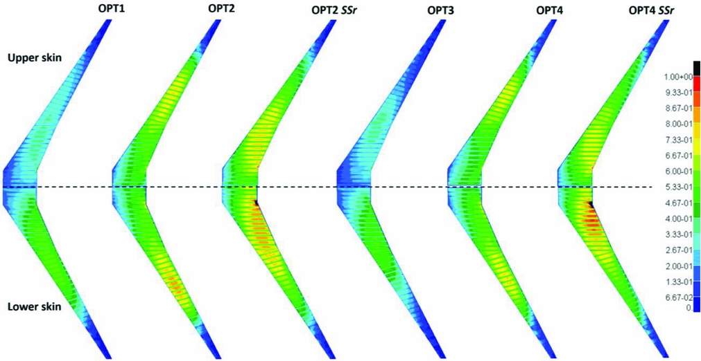
The strain fields on upper and lower skins for the 2.5g load case are shown in Fig. 10, in terms of normalised strains averaged through the shell thickness. Rib strains are, in general, homogenously small when compared to those developed in the skins and, thus, not shown here. Strain fields of the front and rear spars follow approximately the same distribution and magnitude of those observed at the edges of the skins, and similarly are not covered here. Overall, all designs have a strain distribution varying smoothly, with peak values occurring along the wingbox trailing-edge, especially at the fuselage-joint connection and in the wing kink areas. This effect is more evident at the mid semi-span, where the transition in rib orientation occurs. Note that for the composite designs, the KS constraints for principal strains are active in a few grid points of the fuselage-joint connection of the lower skin. Owing to the conservatism of the KS function, and to the fact that the normalised strains shown in Fig. 10 are averaged through the element thickness and grid points, the normalised active strain constraints are slightly less than 1.
KS function for strain distribution.

The allowable strains for the composite skins are substantially lower than those for the all-metallic wings. Consequently, composite designs carry higher normalised strains values (of the order of ~ 0.80 to 0.85). Due to a significant reduction in both shear-extension and bend-twist couplings, OPT2 SSr and OPT4 SSr operate in a more critical load state, where strain and buckling constraints are violated (approximately 5% higher than the maximum allowed), resulting in increased strains spread throughout a larger portion (shifted towards the wing root) of the wing skins. Furthermore, it is noted that there is a difference between some of the lamination parameters and ply percentages matching in Figs 6 and 7, suggesting that the changes in the root to mid-sections (up to 0.4 normalised wing span) are mostly responsible for the structural improvements.
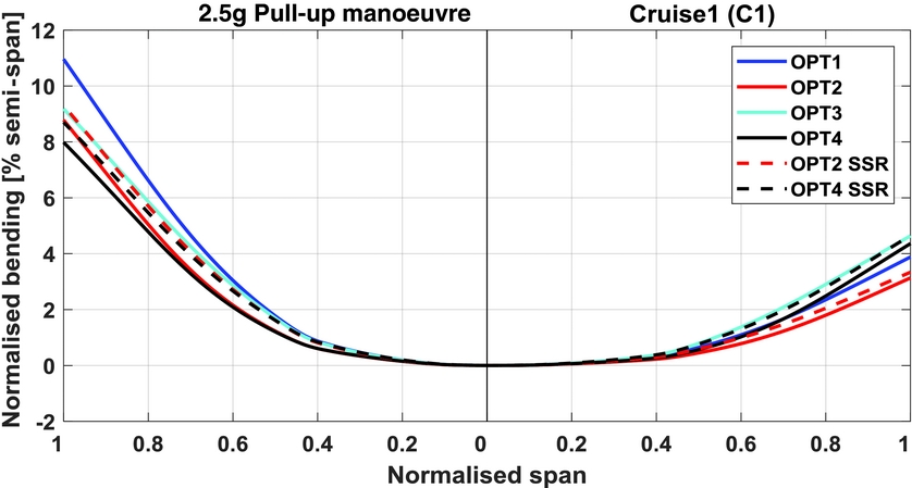
In terms of deflections, Fig. 11 shows that wings actuated by controls deflect more at the cruise condition (C1) than the wings optimised without controls. For load relief, it is observed that both composite wings are less compliant in bending than the equivalent all-metallic wings. Comparing the composite wings and their respective second-level solution, although the influence on the displacement response appears small, the redistribution of strains from the first and second level design is quite important as shown in Fig. 10. This is a result already highlighted in previous studies(Reference Macquart, Werter and De Breuker50,Reference Bordogna, Macquart, Bettebghor and De Breuker51) .
Bending deformations.

6.3 Control deflections, span loads and twist shapes
In flexible wing structures (flying under the control reversal speed), the local lift generated by a streamwise section increases when the flaps are deflected downwards and decreases when upwards-control rotations are given. A tip-down flap increases the nose-down pitching moment about the wing aerodynamic centre, forcing the aircraft to reduce its trim angle-of-attack. Opposite behaviour is observed when a flap is rotated upwards. Generally, a flap deflection changes the aerofoil camber, thereby reshaping the aerodynamic loads and changing the spanwise drag and lift distributions.
Swept-back wings can be more sensitive to positive control deflections (flap rotated downwards), because the structural bend-twist coupling (that can be altered by laminate stiffnesses for the wing with composite skins) will naturally cause the wing to washout. Therefore, the resulting amount of nose-down twist will be the combination of those accompanied by the wing bending deflection and those due to the increase in pitching moment that further increases the wing torsion. This load redistribution can be beneficial from the structural standpoint, because it shifts the centre of pressure further inboard rather than outboard.
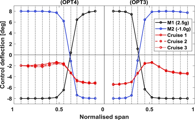
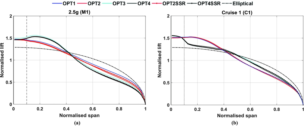
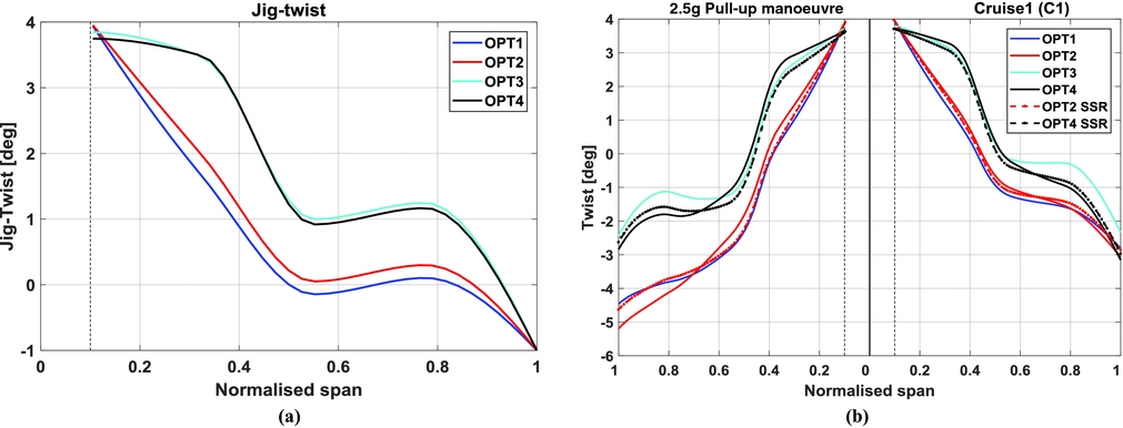
The control displacement layout found by the optimiser is shown in Fig. 12, for all of the cruise segments, along with the 2.5g manoeuvre, and for both the wing with composite skins and the all-metallic structure. The main role played by the deflected controls during cruise alter the aerodynamic moments running spanwise along of the flexible wingbox, increasing the trim angle-of-attack (at constant lift coefficient) by producing more lift outboard, hence, reducing both wing drag and tailplane trim drag. Given the optimised jig-twist input variables and the resulting cruise twist distribution shown in Fig. 14, it is evident that for all of the design cases discussed here, the optimiser attempts to counteract the wing washout (due to the optimised jig-twist) by increasing the outboard streamwise angle-of-attack (wash-in) rotating the majority of the control surfaces upwards (negative deflection). The result is a lift distribution that reaches a more elliptical loading, as seen in Fig. 13, which would minimise the fuel burn.
Optimised control surface deflections for cruise and manoeuvre load cases.

Cruise-climb and 2.5g manoeuvre spanwise lift distributions for OPT1 through OPT4. (a) Spanwise lift distribution for manoeuvre load case. (b) Spanwise lift distribution for cruise 1 load case.

In comparison to the all-metallic wing, the composite one needs less control deflections to achieve similar spanwise efficiency. This finding is thought to be due to the composite wing being more compliant in torsion; it requires a lower degree of wash-in to be produced by the trailing-edge flaps to “pull out” the triangular-shaped lift distribution to one closer to the elliptical shape.
Referring back to Fig. 12, showing the layout of the control displacements for the 2.5g pull-up manoeuvre, one can assume that the optimiser uses negative control rotations outboard (control surface rotated upwards) to reduce the streamwise AoA locally, thus decreasing the amount of lift generated close to the wingtip. Since NASTRAN solution 144 performs a trim analysis, additional lift is then necessary for trimming the aircraft, which is achieved by giving the inner wing controls an upward displacement. This control deflection pattern is close to the one previously found by Stanford(Reference Stanford26,Reference Stanford27) . Intuitively, this loading shape is preferable from a structural perspective because the centre of pressure is shifted inboard, therefore reducing the root bending moment which, in turn, allows for more material to be removed from the wing skins and spars without any structural constraint violation.
Fuel burn, i.e. our objective function, does not depend entirely on aerodynamics with the total structural weight playing an important role in defining the optimal trade-offs between load alleviation and optimised cruise lift efficiency. This effect is shown by the optimised jig-twist shapes of Fig. 14(a), which, for all design cases, wash out approximately by 5° suggesting that the values for the jig-twist shape design variables are mainly dictated by manoeuvre buckling and strain constraints. In general, it is found that the optimised twist shape is set to alleviate loads via a passive washout mechanism, whereas the controls' displacements tend to increase lift outboard in order to reach the minimum-drag spanwise distribution.
Jig-twist and elastic torsional deformations. (a) Jig-twist shape. (b) Elastic twist shape.

Although normalised spanwise loads for the designs with retrieved blended laminates are almost identical to those obtained in the top-level optimisation, a small loss in aerodynamic performance is observed. This loss can be related to a small change in bending and twist deflections (due to smaller bend-twist couplings), that, in turn, degrade the aerodynamic performance due to increased trim drag.
6.4 Optimal wing weight and first-order performance implications
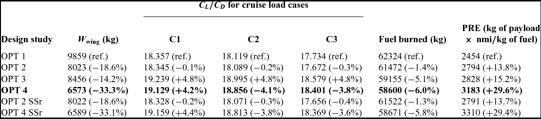
In this section, we examine and quantify the aerostructural performance of the design produced by the optimisation by assessing the total fuel burned (and the associated design metrics necessary for its calculation, e.g. wing structural mass and cruise lift efficiency) and by introducing a Payload-Range Efficiency parameter (PRE)(Reference Nangia52). Optimal design metrics are provided in Table 6 and benchmarked against OPT1 (all-metallic wing with undeflected control surfaces) which is the heaviest solution found. As expected, minimum fuel burn is achieved by simultaneously reducing wing structural mass and improving lift efficiency across the entirety of the cruise mission.
Wing structural weight and first-order performance implications

Higher lift-to-drag ratios are achieved by the optimisation studies that purposefully explore the use of controls to reshape the aerodynamic loads throughout cruising flight. Amongst the passively tailored designs, OPT2 features very similar L/D values when compared to OPT1, though less fuel burn is achieved as a result of the significant lighter structure (18.6% lighter). It is also noted that, for control-augmented designs, lift efficiency increases an average of approximately 4% for each cruise load case in comparison to the passive counterpart designs.
Wing structural mass (for half-aircraft, excluding leading-edge and trailing-edge lumped masses) is also shown in Table 6. One can note that including adaptive controls allows the optimiser to yield, for the all-metallic structure of OPT3, approximately 14% less structural weight than the reference design of OPT1. This difference is about 18% when considering the passive adaptive design of OPT2 and its counterpart, OPT4. Perhaps, greater mass reductions could be achieved if the wing skins were tailored in the chordwise direction as well, allowing for a more local tailoring. Additionally, it is thought that larger control surfaces operating at higher rotations or splitting the flaps into more chordwise and spanwise segments could yield higher lift efficiencies and would also improve weight savings.
Observing the last two rows of Table 6 and referring back to Fig. 10, one can conclude that the differences between designs in lamination parameter space and stacking sequence space result in a small to moderate loss in aerostructural performance. This outcome reinforces the argument that blending constraints should be included in the top-level optimisation.
In addition to fuel burn, another convenient way of judging the cruise performance of transport aircrafts is assessing PRE. This metric can be interpreted as the useful work done (payload × range) per unit mass of fuel consumed and is given according to
 $$\begin{equation}
{\rm{PRE}} = {\rm{payload\ }} \times {\rm{range}}/{\rm{fuel}}\;{\rm{burned}}.
\end{equation}$$
For a fixed MTOW, the difference in wing mass with respect to OPT1 is converted into additional payload and used to estimate the PRE parameter. Overall, both fuel burn and PRE parameter demonstrates the superiority of composite materials over all-metallic airframes clearly, especially when adaptive controls are added to alleviate critical loads and maximise cruise performance showing an improvement in fuel burn of approximately 6.0% in comparison to the reference metallic wing.
It is observed that the optimisation problem studied here is highly non-convex in nature. One could therefore imagine that multiple local solutions could exist. Future work may address this issue by adopting a more robust optimisation approach to better define the optimisation starting point to retrieve global optima.
7.0 CONCLUSIONS
A series of aeroservoelastic wingbox designs is presented that exploit the synergies between passive shape adaptations achieved via elastic tailoring (i.e. variations in thicknesses, jig-twist and stiffnesses) and via adaptive trailing-edge flaps, for manoeuvre load alleviation and enhanced fuel efficiency. The baseline wing is representative of a long-range commercial airliner and features laminated wing skins and a metallic wingbox substructure. Optimisations are conducted using a bi-level approach, which integrates gradient-based and particle swarm algorithms in order to tailor the wing locally and retrieve manufacturable composite stacking sequences.
Both optimised composite designs are largely unbalanced with non-negligible membrane and bending anisotropy. It is further noted that the composite wing with trailing-edge controls exhibits greater in-plane anisotropy more inboard the wing semi-span in comparison to the passively tailored composite wing. In general, designs with retrieved blended laminates show a moderate loss in aerostructural performance associated with greater bending deflections that downgrade lift efficiency. This observation suggests the need of incorporating additional blending constraints in the top-level optimisation.
Since fuel burn does not depend entirely on the wing's aerodynamics, it is found that the jig-twist shape resulting from the optimisation introduces a passive washout mechanism to alleviate loads. Similarly, flaps are used to increase lift outboard, in order to attain the spanwise load distribution that minimises the overall drag. Opposite results are observed when optimising for load alleviation only, which causes the wing's centre of pressure to shift inboard, thereby reducing root bending moment and structural demands.
Amongst the results presented, as expected, the hybrid wing with composite skins and trailing-edge devices outperforms the all-metallic wings clearly both in terms of fuel burn or payload-range efficiency parameter.
This work has demonstrated the improvement of performance of aeroservoelastically tailored composite wings, over traditional designs. Considerable weight savings can be obtained due to manoeuvre load alleviation accompanied by improved lift efficiency (hence, fuel burn) over a realistic flight with multiple cruise conditions.
ACKNOWLEDGEMENTS
This research was supported by the Conselho Nacional de Desenvolvimento Científico e Tecnológico (CNPQ), under the Science Without Borders programme.