

Introduction
Wine consumption per capita in the U.S. has increased by 40% in the last 15 years (Wine Institute, 2015). As wine production continues to increase to keep up with demand, a consistently high quantity and quality grape supply is imperative. California grows over 200 million hectares of wine grapes (California Department of Food and Agriculture, 2015) and produces 90% of the wine in the United States (The National Association of American Wineries, 2014). However, California’s wine grape production capacity is being challenged by other successful and rapidly expanding permanent crops such as almonds and pistachios which compete for the same land, water, and labor resources. While vineyards are slowly expanding into new areas of California with relatively marginal soils but more secure water supply, an important strategic component to securing California’s grape supply consists of maximizing yields in the existing vineyards.
The use of precision agriculture (PA) tools based on soil, yield, or canopy mapping, has greatly improved management practices in agronomic crops, resulting in significant yield and economic increases. Due to the inability of genotype selection on an annual basis, long lived crops such as grapes have not yet benefited from precision agricultural technology. Nonetheless, our understanding of vineyard variability and the tools needed to manage variability have been in development for the last 20 years, with most of the initial work beginning in Australia, followed by Europe, and more recently California (Arnó Satorra et al., Reference Arnó Satorra, Martínez Casasnovas, Ribes Dasi and Rosell Polo2009).
The inefficiency of uniform management has become an issue of interest with broader access and use of sources like soil maps and aerial imagery. Yield monitors have been used in broad acre crops since the 1980s but were not introduced to perennial crops until much later (Cook and Bramley, Reference Cook and Bramley1998). The first grape yield monitor became commercially available in Australia in the 1999 vintage (Bramley, Reference Bramley2001a) but they have only recently been used in California vineyards (Troxell et al., Reference Troxell, Sams, Sánchez and Dokoozlian2014). Yield maps accentuate areas of concern in vineyards and can aid in the delineation of management zones (Tagarakis et al., Reference Tagarakis, Liakos, Fountas, Koundouras and Gemtos2013). Yield maps, in conjunction with soil analysis, remotely sensed variables, physiological and chemical analysis of vines, and other data, can elucidate why particular vines (or sections) produce less fruit than others.
Commercial vineyard management adds complexity to this issue. In vineyards larger than 5–10 hectares, multiple machine harvesters may be needed in order to deliver fruit to a winery in a timely manner. The number of machines and the size of the vineyards necessitate new methods for faster data processing and more efficient management in the field. The objective of this paper is to describe two methods used to process yield data from several hundred vineyards within a short time after harvest.
Materials and methods
Data collection
ATV yield monitor systems (Advanced Technology Viticulture, Adelaide, Australia) were installed on an increasing number of commercial grape harvesters over the course of three years, 2012–2014. Yield maps were completed for the 2015 and 2016 seasons using ATV yield monitors mounted on 50 machines and covering a total of about 5,000 hectares. Each yield monitor is comprised of a weighing scale, a GPS unit, and a data logger. The weighing mechanism consists of two load cells on a frame placed beneath either the discharge belt or sorting belt on each of several models of mechanical grape harvester. The load cells measure the weight of the fruit as it passes over the scale and each weight is tied to a spatial position collected by a differential Trimble AgGPS 162 (Trimble Navigation Limited, Sunnyvale, CA) using the Global Positioning System (GPS). Data from the load cells and GPS unit are merged using ATV proprietary software. Raw values are recorded by a data logger and transferred to a geographic information system (GIS) for map creation.
Yield monitor units are calibrated by comparing weights from grape delivery trucks and the associated sensor weights taken from the yield monitor. Calibrations are normally done by comparing winery test stand weights to sensor weights collected with the yield monitors. A correction factor (CF) can then be adjusted based on the equation below.
 $${\rm New}\,{\rm CF}={\rm CF}\left( {{{{\rm actual}\,{\rm harvested}\,{\rm weight}} \over {{\rm displayed}\,{\rm total}\,{\rm weight}}}} \right)$$
Three yield monitor equipped harvesters were examined to better understand potential “calibration drift” over a single night’s harvest. Sixteen truckloads of 22 MG were scheduled for delivery to the winery on 5 September 2016. Each team of two gondolas, 5.5 MG each, was arranged to empty loads specific to each harvester into individual 22 MG trucks in order to track the sensor signal of each harvester yield monitor to the winery scale. Machine drivers reset the yield monitor to zero after each gondola exchange in order to provide an appropriate marker in the harvest weight data set. Four consecutive gondola weights are taken from the raw yield monitor output file and added together to equal the number of bins in a corresponding truck. Prior to each picking session, each belt is run through a tare process. This process attempts to “zero” each belt by running the belt empty for up to 30 seconds. It is assumed that this tare value remains constant throughout a single night of picking. In this case, four calibration weights were measured over one night for each of the three machines. After harvest is finished in a particular block, the data are extracted and merged into spatially relatable fruit weights.
Method 1
The first method, employed during initial yield mapping efforts in 2012–2013, requires the use of separate grape trucks for each harvester in a given field. Each 22 MG truck carries four grape bins of about 5.5 MG which are filled one at a time by four gondolas. After its four bins are filled, each truck travels to the winery where it is weighed. In order to isolate the signal from each harvester, the user must ensure that all gondolas from a given harvester are emptied into one single truck. Once the data are captured by the yield monitor and merged, the data processing begins. First, data are separated by digital boundaries for each ranch and vineyard. Yield data are first “trimmed” in order to eliminate points outside of vineyard areas and statistical outliers according to Bramley and Williams (Reference Bramley and Williams2001). Next, data are interpolated using a model fit to a semivariogram according to Whelan et al. (Reference Whelan, McBratney and Minasny2002). In this case, a local variogram using an exponential model was calculated from within a neighborhood of least 50 data points and no more than 150 data points.
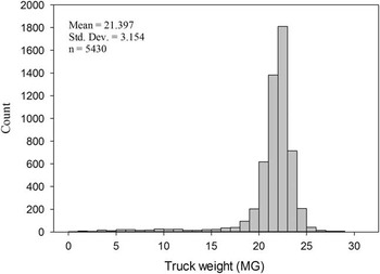
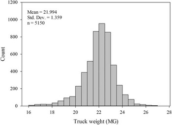
In 2014 and 2015, the calibration to trucks in the field assumed each delivered truck was the mean delivery to the winery, about 22 MG per truck. Figure 1 shows the distribution of truck weights delivered to the winery for a single variety (Cabernet Sauvignon, Vitis vinifera L.) for the 2015 and 2016 harvests. Figure 2 shows a similar distribution, but with trimmed values of the same dataset. Trucks delivered with less than 16.5 MG and more than 27.5 MG were removed. This trimming relies on the assumption that these trucks were not filled with all four gondolas or that an extra gondola was added accidentally.
Distribution of all grape truck weights (MG) delivering a single variety during the harvests of 2015 and 2016.

Distribution of grape truck weights between delivering a single variety during the harvests of 2015 and 2016 after global outliers have been removed.

Method 2
Method 2 still requires some initial calibration to actual weight in the field, but does not rely on the truck tracking in Method 1. This calibration usually only happens once, at the start of the season. Initial data processing occurs using the same process as in Method 1, but with added automation. As with Method 1, data are sorted spatially using digital boundaries for each vineyard. Each harvester signal is then adjusted by comparing the average yield of the vineyard to the average yield of each harvester session as shown by Equation 2. The mean comparison adjusts each signal to the mean weight captured and recorded from the entire vineyard. In doing so, each uncalibrated session of data points is put into the same scale. Each vineyard can then be processed at the same time without user input by multiplying the original values by the correction factor. Maps were created using ArcGIS 10.3 (ESRI, Redlands, CA).
 $${\rm Correction}\,{\rm Factor}=\left( {{{{\rm Average}\,{\rm Vineyard}\,{\rm Yield}} \over {{\rm Average}\,{\rm Harvester}\,{\rm Session}\,{\rm Yield}}}} \right)$$
 $${\rm Corrected}\,{\rm Yield}={\rm Yield}\,{\rm {\asterisk}}\,{\rm Correction}\,{\rm Factor}$$
Results and Discussion
Drift
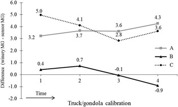
Results from the yield monitor drift study show varied results (Figure 3). The trend for Harvester A is the most stable (total difference of 0.5 MG) and shows consistent drift over four calibration points. The drift in Harvester A is consistently rising but at a relatively slow rate. Harvesters B and C have total differences of 1 MG each but have no consistent pattern. Both B and C drift up and down with different trucks. Total variance in trucks after the rough trim was 1.85 MG. Variance of differences between truck and sensor weight was between 0.1 and 1.5 MG.
Truck weight comparisons over time from three machine grape harvesters over one harvest shift.

Mapping
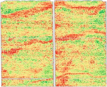
In 2014 and 2015, the maps were created using Method 1, and required approximately 500 hours per year to finish all 5,000 hectares. This includes the time spent in the field calibrating machines and the time spent manually adjusting each harvesters signal to the calibration numbers. In 2016, less than 50 processing hours were needed to finish maps for all 5,000 hectares. Both methods start with a similar problem as shown in Figure 4 and result in a similar product as shown in Figure 5. Both maps were created using the same data from the 2016 harvest season. At a pay rate of $30/hour, the cost of 500 hours needed using Method 1 equals $15,000. At the same rate, 50 hours of work using Method 2 equals $1,500, a reduction of 90%.
Challenges of mapping with multiple harvesters and associated yield signals picking in a single block.

Example of resulting map of vineyard yield from Method 1 or Method 2.

The level of drift in the harvest shift studied was slightly lower than the variance across trucks delivering to the winery. Some of the difference between trucks is very likely due to the range of conditions by which grape trucks are delivered to the winery. Some loads may contain some hand-picked fruit, there may be spillage when emptying gondolas, and growers may over or under load gondolas for various reasons. With production speed and necessity in mind, the average truck weight is assumed in order to adjust weights from each harvester. If this is the case, Method 2 requires less work in order to produce useful maps of grape yield. One downside of Method 2 is that the harvester operator does not necessarily have an accurate weight displayed on the yield monitor data logger.
There was a staffing change between 2014 and 2015 that could have an effect on processing, but is unlikely to be a major factor. Training has occurred with multiple other personnel and time taken to adjust maps using Method 1 is generally about the same. Much of the processing time savings occurred due to the automation of data trimming and the ability to run over night. Time spent in the vineyard with harvesters decreased over time, in part because of fewer manual changes to correction factors, but is not reported here.
Conclusion
Drift in yield monitors is a potential issue but can be mitigated by daily belt calibrations and adequate yield monitor and harvester maintenance. Both mapping methods are effective at creating yield maps, but Method 2 offers a significant reduction in time, both in the field and at the computer.
Acknowledgements
We would like to thank the staffs at Gallo Vineyard Management and Pacific Agrilands for their support in this project. Thank you to Maegan Salinas for creating maps in 2014, to Charlotte Mays for creating maps in 2016, and to Devin Rocco for automation support.