1. INTRODUCTION
The primary choice for almost all outdoor land navigation tasks for vehicles or persons is GPS. In buildings, however, GPS is generally unavailable. One possible solution for indoor personnel tracking is based on Inertial Measurement Units (IMUs). IMUs comprise a 3-axes accelerometer and a 3-axes gyroscope. Both of these sensor modalities require, among other mathematical processing, that their signals be numerically integrated to produce the desired position and attitude information. The numeric integration has a tendency to cause errors due to drift. Drift is produced when small, slow-changing deviations from the correct signal are integrated with respect to time. The highly undesirable result of drift is that the error of the computed output – relative position or attitude – increases continuously and without bound.
One can conceptually view drift as being composed of two components: a slow-changing component, called “bias instability,” and a high-frequency noise component with an average of zero. The error contribution due to the integration of the high-frequency noise component is called “Angle Random Walk” (ARW). Generally, ARW creates only small errors in the computation of heading since its average is about zero. In the context of this paper, we are therefore concerned only with the slow-changing component of drift.
Gyros are also sensitive to changes in temperature, and certain gyros are sensitive to linear accelerations. In our application, these two effects also produce errors that can be treated as having slow changing components, as does drift. Our proposed heuristic drift elimination method counteracts all slow-changing errors regardless of whether they were caused by the physical phenomena of drift, temperature sensitivity, or sensitivity to accelerations. For that reason, in this paper we lump all three of these error sources together and call them collectively “drift.”
Before explaining our proposed drift elimination method in Section 2, we discuss here briefly several others approaches to reducing gyro drift. The most common methods are to integrate IMU and GPS information [Cavallo et al., Reference Cavallo, Sabatini and Genovese2005] [Mohinder et al., Reference Mohinder2002], [Grejner-Brzezinska et al., Reference Grejner-Brzezinska2006]. Cho et al. [Reference Cho, Lee, Park and Lee2003] integrate data from a magnetic compass as well. Basnayake et al. [Reference Basnayake, Mezentsev, Lachapelle and Cannon2005] propose a method that makes use of available maps in combination with map matching techniques for further enhancement. The main drawback of these approaches is that either they required external references or information ahead of time, which may not be available all the time. For example, GPS only works outdoors and magnetic fields are often disturbed and unusable in or near man-made structures. Chen, [Reference Chen2004] tried to find a mathematical model for bias errors, but this technique has limited applicability and can only estimate the deterministic part, if any, of the bias drift.
In earlier work the authors of this paper introduced a method called “Heuristic Drift Reduction” (HDR). HDR makes use of the fact that many streets or corridors are at least partially straight [Borenstein et al., Reference Borenstein, Ojeda and Kwanmuang2009]. At any moment, the HDR method estimates the likelihood that the user is walking along a straight line. If that likelihood is high, HDR applies a correction to the gyro output that would result in a reduction of drift if indeed the user was walking along a straight line. If the algorithm assesses that the user is not walking along a straight line, then HDR does nothing.
The limitation of the HDR method is that at best (i.e., when indeed moving on a straight line), it reduces the effect of drift to nearly zero, so that the measured rate of turn reflects the true rate of turn. During that time, integration of rate of turn yields the correct changes in heading and no new heading errors are produced. When not moving straight, at best we can expect HDR to notice that and suspend its operation. During that time, drift accumulates and the integration of rate of turn results in heading errors. Then, when moving straight again, new heading errors are prevented, but those heading errors that were accrued while HDR was suspended remain in the system and cannot be eliminated. The effect of the HDR method is thus that it reduces heading errors due to drift substantially, but heading errors still grow without bound.
The remainder of this paper is organized as follows. Section 2 explains the new HDE method in detail. Section 3 provides a description of our Personal Dead-reckoning (PDR) system and Section 4 shows experimental results obtained with HDE applied to our PDR system. Conclusions are presented in Section 5.
2. HEURISTIC DRIFT ELIMINATION
In this paper we present our new Heuristic Drift Elimination (HDE) method that not only reduces errors due to drift, as our older HDR method does, but virtually eliminates them. In suitable indoor environments, HDE maintains near-zero heading errors in walks of unlimited duration, at steady state. Steady state is typically reached within a few seconds after walking straight along a corridor. However, these highly desirable performance characteristics are achieved only in environments that match certain heuristic assumptions, discussed next.
2.1. The Heuristic Assumptions
HDE is quite similar to HDR, but far more powerful, because it corrects computed heading angles, not rates of turn. HDE works in environments in which possible heading angles are limited. For example, in man-made buildings most corridors are straight and either parallel or orthogonal to each other and to the peripheral walls. We will call the typical directions of walls and corridors the “dominant” directions of the building. In a huge majority of buildings there are only four dominant directions. One can easily verify this observation by looking at aerial or satellite photos of city and rural buildings: with very few exceptions, residential and business buildings have rectangular footprints, suggesting that most corridors and walls inside follow four dominant directions. Among the rare exceptions, we found empirically that the most frequent one is that of corridors angled at 45° to others. In order to account for this exception, our heuristic assumptions actually allow for eight dominant directions, spaced at 45-degree intervals. Informally, we estimate that well over 99% of all man-made structures have four or eight dominant directions. Prominent exceptions are the Pentagon, some architectural landmarks such as theatres, opera houses, and large hotel complexes, and indoor sports arenas. HDE cannot be used in these exceptional environments.
In all other, “normal” environments, where most walking happens along dominant directions, HDE gradually corrects the gyro output so that the combined effect of drift and HDE correction is such that the computed heading matches the closest dominant direction. When the walker turns, HDE suspends its corrective action. While HDE is suspended, drift causes new heading errors, as it does with HDR. However, once HDE resumes, it effectively eliminates accrued heading errors because it gradually forces headings to be aligned with the closest dominant directions. Therefore, HDE bounds heading errors and keeps them near zero in walks of unlimited duration – as long as most of the walking happens along dominant directions. We call walking that complies with the heuristic assumptions (i.e., walking along a dominant direction) “compliant” walking. The strength of HDE lies in the fact that it applies corrections very gradually. As a result, short stretches of non-compliant walking don't cause problems, while prolonged compliant walking gives the gradual corrections enough time to be effective.
HDE works generally with any personal tracking system that uses one or more gyros for measuring rate of yaw to compute the user's heading. One such personal tracking system is the so-called “Personal Dead-reckoning” (PDR) system that we developed in earlier work. However, the focus of this paper is not on the PDR system itself. For that reason and in order to avoid distraction from the general applicability of the proposed HDE method, we defer a description of our PDR system to Section 3.
2.2. General heading estimation
Suppose a person is steadily holding a z-axis gyro while walking straight forward on level terrain. Moving straight forward, the output of the z-axes gyro should be exactly zero throughout the walk. However, due to drift the actual output is off by some small value ε. Suppose further that we divide the total travel distance into smaller intervals. A natural choice for the length of an interval in a pedestrian tracking application is from footfall to footfall. We define “footfall” as a single instance in which the IMU-equipped foot is firmly in contact with the ground and the forward velocity of the shoe at the contact point is zero. Since only one foot is instrumented, there are two steps between footfalls.
Due to the drift error ε, in each interval the rate of rotation computed based on the z-axis gyro is:

where
- ωraw –
Rate of rotation measurement. This is the direct output of the gyro.
- ωtrue –
True but unknown rate of rotation.
- ε0 –
Static bias drift, measured immediately prior to a walk while standing still.
- εd –
Bias drift. This is the unknown slow-changing drift component.
Immediately prior to each walk and with the gyro held completely motionless, the static bias drift ε0 is measured by averaging T bias seconds worth of gyro data. The value for T bias depends on the quality of the gyro and can be estimated by using the Allan Variance analysis [Ferre-Pikal et al., Reference Ferre-Pikal1997]. T bias is also called “bias time.” In our system, T bias=25 sec.
During the walk, ε0 is subtracted from every reading of ωraw:

Then, the new heading ψi is computed:

where
- ψi –
Computed heading at footfall i, in [°].
- ωmeas,i –
ω after removing static bias drift, in [°/sec].
- T i –
Duration of time interval i in [sec]. T i is the time between footfall i-1 and footfall i.
When walking straight forward, ωtrue=0, and ψ=εdT i. If we further assume that the walking happens along the first of the four or eight dominant directions, which we define as being aligned with 0°, then ψi should be zero. If it is not, then it must be so because of drift, εd.
In general terms, HDE works as follows. After each footfall, HDE examines ψi and issues a small drift correction based on the sign of ψi. If after the next footfall ψi+1 still has the same sign, then HDE issues another correction, and so forth, until after n footfalls the sign of ψi+n is reversed.
In the following sub-sections we explain in detail how the HDE algorithm:
• reduces walking in any of the nominally four or more dominant directions to the functional equivalent of walking in a direction of zero degrees;
• models εd as a disturbance in a feedback control system;
• estimates the magnitude of this disturbance by examining the content of the accumulator in the I-controller of that feedback control circuit;
• remains largely insensitive to changes in ψ that have large-amplitudes but short duration.
2.3. The Basic HDE Method
As explained, the HDE algorithm assumes that a building has four or eight dominant directions, Ψ. In order to keep the discussion in this section intuitive, we will explain HDE for four dominant directions. In that case, dominant directions are spaced at 90-degree intervals and we call this interval the “dominant direction interval,” Δ. Mathematically, Δ can have any value, but in practice performance degrades for Δ<45°. A further assumption is that most walking in such buildings happens along dominant directions. HDE can tolerate some exceptions, for example, when performing a task in a room, when crossing a large room at an angle, or when turning around a corner.
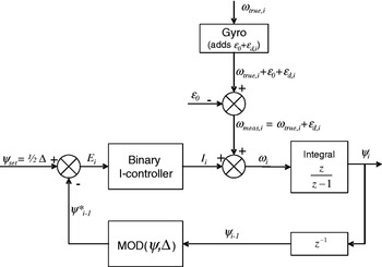
The basic HDE algorithm functions essentially like a feedback control system. This is different from most other measuring systems, where signals pass from the sensor to the instrument's output in open-loop fashion. Figure 1 shows a block diagram of the feedback control system for the HDE algorithm. Before we explain the overall function of this feedback control system, it is necessary to define in detail the function of the block labelled “MOD(θ,Δ).”
The HDE algorithm viewed as a feedback control system. The binary I-controller and the block labelled ‘MOD’ are explained in the narrative.

2.3.1. Use of the MOD function
A “MOD” function is available in different programming environments, but we found that its definition varies, especially with regard to treating negative numbers. In the context of this paper we use the implementation found in Microsoft Excel. In Excel, the MOD function has two arguments, (n, d). MOD(n, d) returns the remainder after n is divided by d, and the result has the same sign as d. In programming environments, in which the MOD function performs differently, the Excel version can be emulated by this formula:

Where INT(r) is a function that rounds a real number r down to the nearest integer. For example: INT(−0·3)=−1.
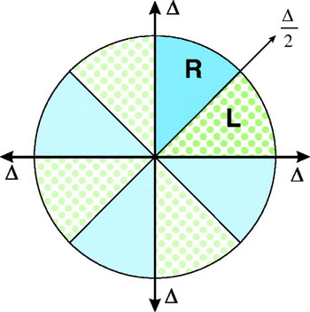
When n and d are angles in the Cartesian coordinate system used throughout this paper, then MOD(n,d) performs a highly useful function: it maps an angle of any magnitude n onto a sector that is bounded on one side by the positive x-axis and that has a central angle of d. As an example, consider the two sub-sectors labelled ‘R’ and ‘L’ in Figure 2. Together, these two sub-sectors form a sector with a central angle of d=90° that coincides with the first quadrant of a coordinate system. The function MOD(n,90°) maps any angle n, which may be greater than 360° or negative, onto Sectors R and L. Similarly, MOD(n,45°) maps any angle n onto Sector L.
Angle mapping with the MOD function.

In the proposed feedback control system of the HDE algorithm, block MOD(θ,Δ) with Δ=90° maps any heading angle onto either Sub-sectors R or L of Figure 2. The functional significance of applying MOD(θ,Δ=90°) is this: In a building with the four dominant directions Ψ=90°, 180°, 270°, and 360° (=0°) any momentary heading direction θ that is immediately to the right of any of these four dominant directions will be mapped into Sub-sector R. Similarly, any heading direction that was immediately to the left of any of these four dominant directions will be mapped into Sub-sector L. With “immediately to the right” we mean angles that are between Ψ and Ψ-Δ/2 (the solid blue sectors in Figure 2), while “immediately to left” means between Ψ and Ψ+Δ/2 (the dotted green sectors in Figure 2).
The significance of the MOD function is that walking along any dominant direction becomes equivalent to walking along the primary dominant direction of 0° degrees. If the walker is off by x degrees to the left or right of any dominant direction, then after applying the MOD function this is equivalent to being off by x degrees from the primary dominant direction. Table 1 illustrates how with the help of the MOD function we can perform a simple test to see if a momentary heading angle is immediately to the right or left of any dominant direction.
Significance of θ*=MOD(θ,Δ) with regard to dominant directions.

2.3.2 The HDE Feedback Control System
We start the explanation of the feedback control system with the signal from the gyro, which was modelled as a disturbance in the block diagram of Figure 1. For the purpose of explaining the feedback control system, let us assume that the user is walking straight ahead and in a dominant direction. We will discuss how the algorithm handles cases when this assumption is not true later. When walking straight, ωtrue=0, so the only output from the gyro, after subtracting the static bias drift ε0, is drift, εd.
This signal is added to the output of the binary I-controller, which will be explained later in this section. Initially, the output of the I-controller is zero, so εd is passed through to a numeric integrator, which computes the relative change of heading, ψi.
After the first iteration, when i>1, the control loop can be closed by submitting the previous value of ψ, ψi−1, to the MOD function. The label ‘z −1’ in the feedback loop is the common notation for a pure delay of one sampling interval. As explained before, MOD(ψ,Δ) maps θ onto a direction that lies between 0 and Δ.

where ψ*i – Mapped heading that lies between 0 and Δ, in degrees.
ψ*i is then compared to the fixed set point, ψset=Δ/2, resulting in an error signal

This brings us to the binary I-controller. Unlike conventional integral (I) or proportional-integral (PI) controllers, the binary I-controller is designed not to respond at all to the magnitude of E. Rather, it only responds to the sign of E. If E is positive (i.e., heading points to the left of a dominant direction), then a counter (called “Integrator” or “I”) is incremented by a fixed small increment, i c. If E is negative (i.e., heading points to the right of the dominant direction), then I is decremented by i c. In this fashion, and although the controller does not respond to the magnitude of E immediately, repeated instances of E having the same sign will result in repeated increments or decrements of I by i c.
The reason for using a binary I-controller is that Ψ* can differ from zero by tens of degrees, for example, when the walker is turning. In that case a conventional I-controller does not work well, since it would respond strongly to the large value of E, even though a large E is not necessarily an indication for a large amount of drift. The proposed binary I-controller, on the other hand, is insensitive to the magnitude of E. Rather, the controller reacts, slowly, to E having the same sign persistently.
As established by equation (6), if ψ*>ψset then ψ* is immediately to the right of Ψ, and if ψ*<ψset then ψ* is immediately to the left of Ψ. During straight-line walking along a dominant direction Ψ, a heading to the right of Ψ suggests that the only possible source for this error, εd, had a negative value. To counteract this error, the binary I-controller adds the small increment, i c to the Integrator. Conversely, if ψ*<ψset, then the Integrator is decremented by i c.
We can now formulate the binary I-controller
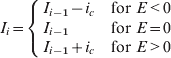
where i c – fixed increment, also considered the gain of the binary I-controller in units of degrees.
An alternative way of writing equation (7a) is:

where SIGN() is a programming function that determines the sign of a number. SIGN(x) returns ‘1’ if x is positive, ‘0’ if x=0, and ‘−1’ if x is negative.
The next element in the control loop adds the controller output to the raw measurement:

where ωi – Corrected rate of rotation [°/sec].
In practice, though, neither ωtrue nor εd are known. Instead, we only know the measured ωmeas,i=ωtrue,i+εd,i. We rewrite equation (8) accordingly:

Substituting equations (5) and (7b) in equation (9) yields:

2.4. Refinements to the Basic HDE Algorithm
Up to this point we have discussed the basic HDE algorithm under ideal conditions. In practice, however, two types of detractions are encountered: (1) measurement noise and (2) walking in non-dominant directions.
2.4.1. Measurement Noise
The PDR system samples the foot-mounted IMU at a rate of 150 Hz and computes the trajectory of the foot during each step. In addition, the PDR system computes the X-Y-Z coordinates of the instrumented foot at each footfall. From any two consecutive X-Y positions of the instrumented foot at footfall the walker's momentary heading can be computed. Lastly, from the change in heading between consecutive footfalls the system computes the walker's rate of turn, ω. The thus-derived ω is treated by the HDE algorithm as though it was produced by an imaginary single Z-axis gyro as depicted in Figure 1. We will use the term “virtual gyro” to refer to the above process that supplies the HDE algorithm with rates of turn at footfall intervals.
The output from this virtual gyro is not constant; rather it varies in a somewhat random fashion at a single, near-constant dominant frequency. This dominant frequency is that of individual footfalls, roughly 0·8 Hz. A secondary source of rate variations is the result of swaying. When persons walk in structured environments, they correct their heading slightly and periodically based on visual cues from the environment. Such corrections happen at the rate of once every few footfalls and their frequency is thus less than 1 Hz. We can consider and will refer to these signal variations as rate noise in the virtual gyro.
In order to cope with the noise of the virtual gyro, it is essential to apply a strong low-pass filter to ωraw. We determined that a double low-pass filter with a time constant of τ>10 sec (i.e., a cut-off frequency of f c=1/τ<0·1 Hz) is effective at smoothing out much of the noise that is specific to our virtual gyro. The two stages of the filter are implemented as:
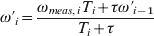
and
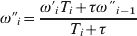
where
- T i –
Time interval, here the time since the previous footfall
- ω′, ω″ –
Rate of turn after the first and second stage of the double low-pass filter, respectively.
2.4.2. Attenuator(s)
The basic HDE algorithm as described in Section 2.3 works very well even in the presence of short stretches of walking in non-dominant directions. For example, turning corners or walking across an open indoor space at some arbitrary angle is possible without degrading performance significantly.
However, if more than, say, 30–60 seconds are spent on walking in non-dominant directions or in arbitrary patterns, then HDE may make “corrections” that are actually damaging. To avoid this pitfall, we introduce an adaptive gain function. With this function, the nominal gain, i c, is reduced in proportion to certain adverse conditions. This is accomplished by multiplying i c with one or more so-called attenuators in every iteration. The attenuators can change between 0 and 1. If no adverse conditions exist, then the attenuators are all set to ‘1’, thereby leaving the gain unchanged. If one of the attenuators is set to ‘0’, then i c becomes zero and HDE error correction is effectively suspended during that interval. In this section we describe one such attenuator, called “step-size attenuator.” Additional attenuators can be designed easily and as needed for particular applications, but all experimental results in this paper are based on using only the step-size attenuator.
The step-size attenuator is based on the assumption that when walkers make particularly short steps, then they are quite likely to be engaged in an activity other than walking along straight corridors.
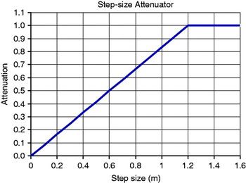
We chose the simple function plotted in Figure 3 for the step-size attenuator:
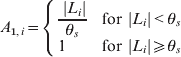
where
- A 1 –
Step-size attenuator, dimensionless, computed after every footfall
- L i –
Step-size in metres
- θs –
Step-size threshold, a tunable parameter
Profile for the step-size attenuator.

2.4.3. De-lagging
The HDE-corrected rate of turn, ωi, as computed by equation (10), still has one problem: The double low-pass filter of Section 2.4.1, which was needed to remove swaying and walk-related oscillations prior to submitting the signal to the HDE feedback control system, leaves ωi with a significant lag behind the raw ωi. If left this way, the subject's trajectory based on ωi would be a rather inaccurate representation of the true trajectory, as sharp turns become prolonged curves. However, this problem can be solved by reversing the effect of the double low-pass filter. To this end, we invert equations. (11a) and (11b):

and

where ωd,i – The final, HDE-corrected and de-lagged rate of turn.
We can now compute the corrected heading by rewriting equation (3):

where
- ψ0 –
initial heading at the beginning of the walk
and the trajectory:


where x 0, y 0 – initial position of the subject.
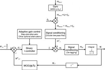
A block diagram of the complete HDE system is shown in Figure 4.
Final block diagram of the complete HDE feedback control system.

3. THE PERSONAL DEAD-RECKONING SYSTEM
We tested the HDE algorithm under real-world conditions with our Personal Dead-reckoning (PDR) system. Before we present the experimental results in Section 4, we offer a brief description of the PDR system.
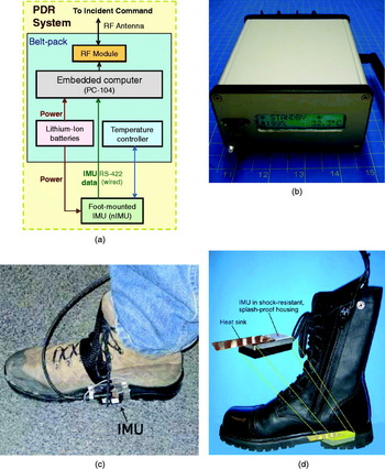
Figure 5a shows a block diagram of the PDR system, which we developed in earlier work at the University of Michigan [Ojeda and Borenstein, Reference Ojeda and Borenstein2007b]. The system comprises an Inertial Measurement Unit (IMU) and a belt-pack that holds a computer, Lithium-Ion battery pack, and custom electronics (shown in Figure 5b). The IMU can be strapped to the medial side of the user's right shoe (to allow transfer of the IMU from one user to another), or the IMU can be embedded in the heel of a boot, as shown in Figure 5c and d, respectively.
The current prototype of the Personal Dead-reckoning (PDR) system. (a) Block diagram of the PDR system; (b) belt pack (Size: 5″×4″×2″); (c) Memsense nIMU unit is strapped to user's boot. The strap-on configuration is good for testing but not for ultimate use by firefighters. (d) IMU built into the heel of a boot. This configuration is impractical for testing on different users but more robust for end users.

A foot-mounted IMU is somewhat of an inconvenience because of the need for power and data wires running up to the belt-pack. However, mounting the IMU on the foot allows the use of a method known as “Zero Velocity Update” (ZUPT) to reset the drift in the accelerometers. ZUPT works for foot-mounted IMUs because during every footfall, when the foot is firmly on the ground, the velocity of the sole at that point is zero. If velocity computed from the accelerometers is not equal to zero, then the accelerometers must be wrong and we can compute by how much the accelerometers are erring. With our implementation of ZUPT and some additional signal processing we achieve consistently errors of 1% of distance travelled. A system similar to ours but apparently developed independently is described in [Yun et al., Reference Yun, Bachmann, Moore and Calusdian2007].
One problem with the PDR system is that we can apply ZUPT only to the accelerometers, but not to the gyros in the foot-mounted IMU. This is because ZUPT requires a reference signal one level of integration above the signal to be corrected. In the case of rates, this reference signal would be angle. It is not possible to measure gyro bias instability during footfalls either, because at footfall, gyro data is too noisy to get representative measurements of bias instability. With regard to tilt, we can bound roll and pitch errors by tilt data provided by the accelerometers during footfall. However, with regard to heading, there is no good method for estimating or otherwise reducing the effects of drift. It is this limitation of the IMU's heading estimation that motivated the present work in the first place.
The IMU used in our PDR system is the nano-IMU (“nIMU” in short), a MEMS-based unit made by [Memsense]. Some key specifications for that IMU are listed in Table 2. The nIMU's gyros work on the basis of the Coriolis Effect. A limitation of low-grade Coriolis-based gyros is that they can be fairly sensitive to linear accelerations [Ojeda and Borenstein, Reference Ojeda and Borenstein2007a]. Due to the relatively high accelerations on the foot during walking, errors induced by this effect can be many times larger than errors due to drift alone. This must be kept in mind when examining the experimental results in Section 4, where uncorrected errors (i.e., result from the standard PDR system without HDE corrections) are notably larger than what can be explained by the nIMU's estimated bias instability parameter of 80°/hr alone (see Table 2). Another problem with the nIMU is its sensitivity to temperature variations, which are especially noticeable when mounted on the outside of the user's boot, where the unit is exposed to ambient air.
Key specifications of the Memsense nIMU.

Correcting for sensitivity to linear accelerations is difficult because of the complex spatial motion performed by the foot during walking. However, it is reasonable to assume that the acceleration sensitivity, which follows similar patterns during each step, can be averaged over several steps and considered as a near-constant – but unknown – disturbance, as long as the user's gait stays the same. When the user changes gait, then the value of that near-constant disturbance changes. For this reason, the acceleration sensitivity acts much like gyro drift. The HDE method successfully reduces these large errors regardless of whether they were caused by drift alone or by the combined ill-effects of drift and acceleration sensitivity. Similarly, since temperature changes are gradual, their effect on the gyros can also be treated as drift and compensated for with the HDE method.
4. EXPERIMENTAL RESULTS WITH THE HDE AND THE PDR SYSTEM
This section presents experimental results obtained with HDE implemented in the PDR system of Section 3. We performed eight long indoor walks, with an average duration of 36 minutes and an average walking distance of 2,167 m (1·35 miles). All walks were performed indoors, in typical university buildings. The buildings are interconnected and happen to have identical dominant directions. When adjacent buildings do not have identical dominant directions, then HDE must be re-initialized for each building before entering it.
Each walk started with 25 seconds of standing still, to compute static bias drift ε0. Then, to initialize HDE, the walker had to walk eight steps straight along a dominant direction of the building. Doing so defines the +Y axis of the PDR/HDE internal coordinate system and one of the eight dominant directions. After the initial eight steps, the subject walked at normal walking speed and gait. In each walk the subject started and stopped at the exact same location. This allowed us to compare the HDE-computed return position with the actual return position and specify a “Return Position Error”. The RPE is less than ideal for specifying position errors, but obtaining ground truth position data for a combined ~11 miles of indoor walking would have been prohibitively time consuming. We did, however, estimate ground truth for heading, at least during steady state. This is relatively simple since we only have to look up the heading of a corridor on a floor plan once, for the duration of the traverse of that corridor. However, whenever the subject turned around corners or crossed wide open indoor spaces we could not estimate ground truth.
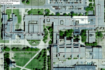
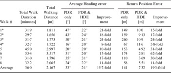
Figure 6 shows the HDE-corrected trajectory of one typical walk plotted over an aerial photo of the five interconnected buildings that were traversed in this walk. Table 3 shows a summary of results for all eight walks. Additional, detailed experimental results are available at our web site at: http://www.engin.umich.edu/research/mrl/PDR-HDE_Detailed_Experimental_Results.pdf
Trajectory of Walk #8 overlaid on an aerial photo of four interconnected buildings at the University of Michigan. This walk took 32 minutes and was 2,065 m (1·3 miles) long. The final position error was 5·5 m and the absolute average heading error was 2·2°.

Average heading errors and return position errors for eight walks.

* In these so-called “Challenge Walks” the subject performed tasks other than just walking along corridors (see narrative).
As explained earlier, extensive non-compliant walking can cause the HDE algorithm to fail. In order to test the resilience of HDE to non-compliant walking, we asked our subjects to perform so-called “Challenge Walks” that included the performance of semi-realistic tasks, besides just walking along corridors. One such task, meant to emulate the action of a first responder, was to enter into as many rooms as were accessible along the way, and to search for would-be victims. To perform this task, the subject walked around in each room as much as needed to look behind furniture and other large objects behind which an unconscious victim might be laying. Challenge walks are marked with an asterisk in Table 3. In all four challenge walks HDE corrected the heading errors that were incurred while performing the challenge task. However, return position errors were on average 2–3 times larger than in simple compliant walks.
5. CONCLUSIONS
In this paper we proposed the Heuristic Drift Elimination (HDE) method for eliminating errors due to drift, variations in temperature, and sensitivity to linear accelerations in a personal dead-reckoning system. The HDE method works only in structured indoor environments, where the basic heuristic assumptions apply most of the time. These assumptions are that most walking happens along straight corridors and that corridors are parallel or intersect at angles that are multiples of 45°. The feedback control loop approach in our system treats drift and other slow-changing errors as disturbances and, just like conventional PI feedback control systems do, eliminates these errors in steady state. After turning around a corner, steady state is typically reached after just a few steps in the direction of the new corridor. Our system differs from conventional PI control systems in that it uses a binary integrator, which makes the system sensitive to prolonged deviations from dominant directions, but not to sudden, large deviations. The unique innovation in our patent pending HDE method is that in appropriate indoor environments, such as almost all residential and commercial buildings, it reduced heading errors to near-zero in steady state and corrects already incurred errors.
On an abstract level, one can say that HDE uses landmarks (i.e., man-made straight-line and right-angle features), but there is no requirement that the location or direction of these landmarks be known in advance and there is no need for another sensor component to track these features. Besides the application described here, we have successfully applied the HDE method to dead-reckoning with Segway scooters and tele-operated robots indoors.
ACKNOWLEDGEMENTS
This material is based on work supported by the U.S. Dept. of Energy under Award No. DE FG52 2004NA25587, by TARDEC through the Ground Robotics Reliability Center (GRRC), by Robotic Research, LLC, and by the Center for Commercialization of Advanced Technology (CCAT).